An Experimental Method for Generating Shear-Free Turbulence Using Horizontal Oscillating Grids


1
National Inland Waterway Regulation Engineering Research Center, Chongqing Jiaotong University, Chongqing 400074, China
2
Key Laboratory of Ministry of Education for Hydraulic and Water Transport Engineering, Chongqing Jiaotong University, Chongqing 400074, China
*
Author to whom correspondence should be addressed.
Water 2020, 12(2), 591; https://doi.org/10.3390/w12020591
Submission received: 7 January 2020
/
Revised: 4 February 2020
/
Accepted: 18 February 2020
/
Published: 21 February 2020
(This article belongs to the Section Hydraulics and Hydrodynamics)
Abstract
:An experimental apparatus driven by horizontal oscillating grids in a water tank is proposed for generating shear-free turbulence, which is measured using Particle Image Velocimetry (PIV). The performances of the proposed apparatus are investigated through the instantaneous and root-mean-square (RMS) velocity, Reynolds stress, length and time scale, frequency spectra and dissipation rate. Results indicate that the turbulence at the core region of the water tank, probably 8 cm in length, is identified to be shear-free. The main advantage of the turbulence driven by horizontal oscillating mode is that the ratios of the longitudinal turbulent intensities to the vertical values are between 1.5 and 2.0, consistent with those ratios in open-channel flows. Additionally, the range of the length scale can span the typical sizes of suspended particles in natural environments, and the dissipation rate also agrees with those found in natural environments. For convenience of experimental use, a formula is suggested to calculate the RMS flow velocity, which is linearly proportional to the product of oscillating stroke and frequency. The proposed experimental method in this study appears to be more appropriate than the traditional vertical oscillating mode for studying the fundamental mechanisms of vertical migratory behavior of suspended particles and contaminants in turbulent flows.
1. Introduction
Turbulence exists widely in river, coastal and ocean environments. Shear-free turbulence is a crucial building block in understanding the fundamental turbulence mechanisms and particle–turbulence interactions. For many decades, shear-free turbulence has been generated in laboratory using different methods. The first way appears to be with a mean flow passing through a grid or mesh in tunnels [1], while such generated turbulence decays rapidly, resulting in small observation time and limited practical utility. As alternatives, researchers have employed a water tank in which the flow is stirred by means of oscillating grids [2,3,4,5,6,7,8,9,10], loudspeaker cones [11,12,13], rotating elements [14] or synthetic jets [15,16,17,18,19]. The oscillating grid turbulence (OGT) exhibits fine homogeneity in planes parallel to the grid and can be easily controlled by varying the operational parameters. Since Rouse (1939) first used OGT to study sediment suspension [20], the OGT was employed to explore the mechanics of the sediment transport [21,22], the interfacial mixing in stratified flows [2,23], the mass transfer across a shear-free water–air interface [24,25], the desorption of contaminants from sediment [26,27], the rate of frazil ice growth [28] and the turbulent thermal diffusion effect [6]. With so many application experiences, despite the emergence of the alternative loudspeaker and jet approaches which are relatively expensive, the OGT was still widely used in recent years [5,29,30,31,32,33,34].
The experiences for single-grid OGT suggested that, to ensure the generation of shear-free turbulence, the grid would have a solidity (defined as the ratio of the area of bars to the total area of the grid) less than 40% [35], the virtual origin was 1–2 cm lower than the mid-position of the grid [36], the oscillating frequency had a upper limit of about 7 Hz [5], the measurements would be initiated after 20 min of oscillation to reduce the influences of initial condition [37] and the distance from the shear-free region to the virtual origin would be more than three times the mesh size [37]. Besides, the relationships between turbulent intensity levels and operation parameters were proposed [2]:
where u and v are RMS velocities in the X and Y directions vertical to the oscillation; w is RMS velocity in the oscillation direction Z; q is RMS of fluctuating velocity; M is mesh size defined as the distance between the centers of two neighboring openings; s is oscillating stroke; f is oscillating frequency; z is the distance from the “virtual origin”; C1,2,3 are coefficients; and n approximately equals to one. Equation (1) was widely used with different coefficients and exponents, and the ratio of C1 to C2 is approximately 0.8–0.9 [4,6,37].
Despite the good planar homogeneity, the single grid turbulent intensity decays rapidly away from the grid, while this can be improved by employing multi-grids [7,38,39,40,41]. It was indicated that, by using two parallel grids, decay of the turbulent intensity reduced with the increasing distance from the grids, and shear-free turbulence was generated in the core region between the grids. The relationship between turbulence intensities and operational parameters was similar to Equation (1), but with different coefficients and exponents [40].
Although the OGT has been extensively studied as elaborated above and listed in Table 1, vertical oscillating grids were usually adopted in these previous studies, resulting in that the longitudinal turbulent intensity was distinctly smaller than the vertical value. On the contrary, the longitudinal intensity was found usually bigger than the vertical intensity with the ratios being approximately between 1.5 and 2.0 in open-channel flows [42]. Additionally, the inertial influence on vertical migratory behavior was introduced due to vertical oscillation [43,44]. These indicate that the OGT generated by vertical oscillating mode may not be fully applicable to the context of vertical migratory behavior in natural flow environments.
The objective of this study is to propose an experimental method to generate shear-free turbulence using horizontal oscillating grids in a water tank. It is expected that such generated turbulence is still shear-free but more consistent with those found in natural flow environments, and hence the proposed method would be more appropriate than the traditional vertical oscillating mode for studying the fundamental mechanisms of vertical migratory behavior.
2. Experimental Apparatus and Set-Up
2.1. Oscillating Grid System
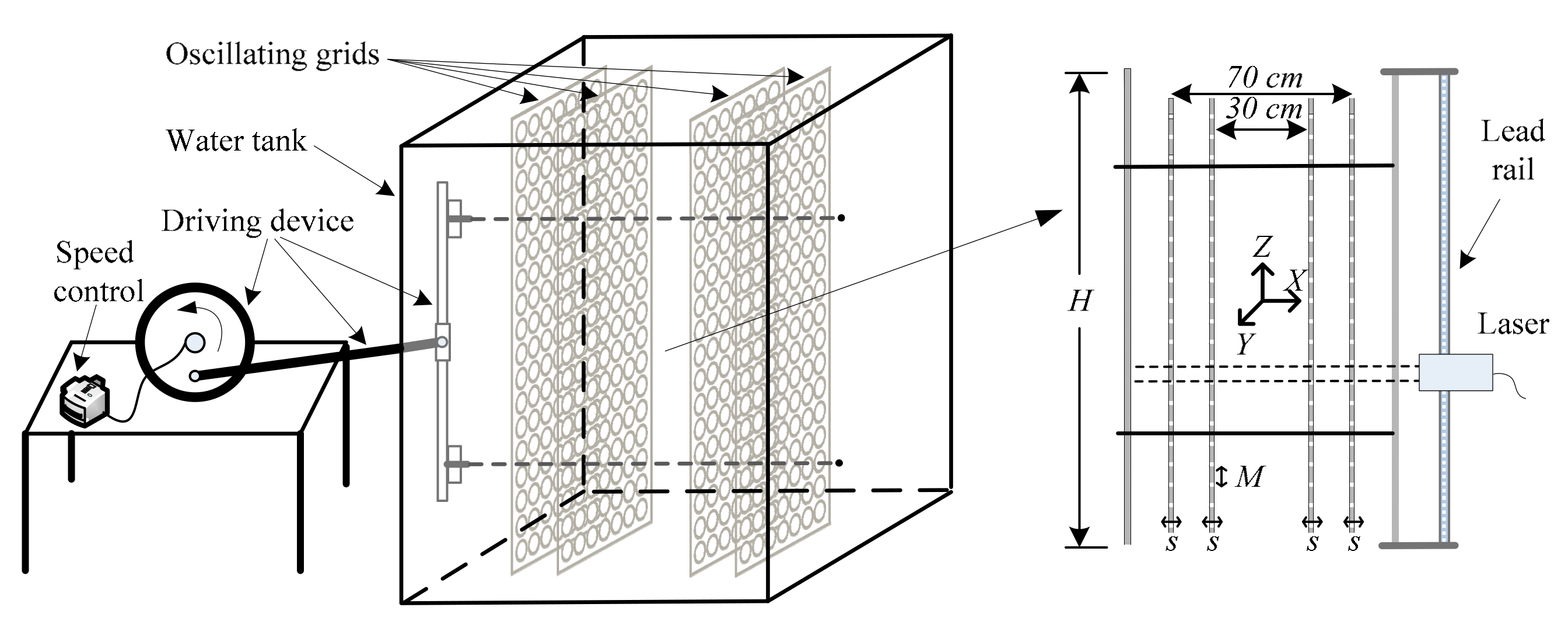
The schematic structure of the experimental system is shown in Figure 1. The water tank has dimensions of 100 cm × 100 cm in the horizontal cross-section and 200 cm in height. The sidewalls of the water tank are built using transparent glass to allow the projection of laser sheets as well as the Particle Image Velocimetry (PIV) measurements.
It has been illustrated in previous studies that the longitudinal turbulent intensities were always smaller than the vertical values of the vertical oscillation generated OGT, and the ratios of these two intensities were usually between 0.8 and 0.9. Considering that the ratios in open-channel flows were approximately between 1.5 and 2.0 [42], a horizontal oscillation structure was adopted to achieve more realistic ratios, and hence can also eliminate the inertial influence on vertical migratory behavior. Four vertically oriented parallel grids, with the distance being 30 cm between the two middle grids and 70 cm between the two outer grids, were coupled symmetrically to a horizontal oscillating driving device, where stroke varies from 0 to 5 cm and frequency varies from 0 to 5 Hz. The grid mesh consists of circular holes with a diameter of 8 cm and the mesh size was 10 cm, obtaining a solidity of 49.8%. Noting that, compared with the conventionally used value, a bigger solidity in this study was to expect that the ratio of longitudinal intensity to vertical intensity can be closer to 1.5–2.0. The grids were made of steel with a length of 80 cm, a height of 180 cm and a thickness of 2 mm, generating a 10 cm gap between each sidewall of the water tank and the edge of the grids, to avoid the influence of secondary flow.
2.2. PIV System
The measurements were taken using PIV, which has the advantages of planar measurements and non-intrusiveness compared with hot-film, LDV and ADV. A continuous laser with a power of 8 watts was used to produce a laser sheet with a thickness of 1 mm through the Powell lens for illumination. Flow tracers are hollow glass particles, with a mean diameter of 10 μm and a density of 1.03 g/cm3. The CMOS camera configured with a Nikon 50 mm f/1.8 D lens was used for image acquisition with the resolution being 2560 × 1920 pixels. The images were processed in an in-house PIV software with a multi-pass and multi-grid window deformation algorithm. The initial and final interrogation sizes were 64 × 64 pixels and 16 × 16 pixels, respectively, with a 25% window overlap. The resultant velocity fields of each iterative stage were validated using the normalized median test, and outliers were replaced by Gaussian-kernel weighted interpolation. The validated velocity fields were then smoothed before the next iterative stage to prevent the possible unstable behavior of the interrogation process. The diameter of the tracer particles in the images was about 4–6 pixels and about 2–4 particles exist in the final interrogation windows.
The PIV used in this study has two data sampling ways, which were independent sampling and continuous sampling. A pair of images is sampled each time and saved to the hard disk with a frequency of 1.5 Hz by using the independent sampling, and one flow field was calculated using this pair of images. One image was sampled each time and saved to the memory card with a frequency of 1000 Hz when adopting the continuous sampling, and one flow field was obtained using every two adjacent images. It should be noted that the time duration of continuous sampling was relatively short due to the restriction of the memory capacity, while that of independent sampling can be much longer.
2.3. Experimental Set-Up
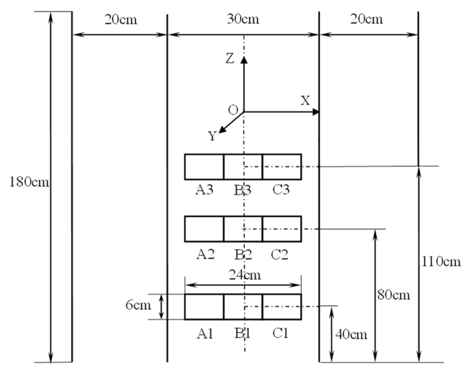
The OGT is sensitive to initial conditions [45], and data acquisition was usually conducted 20 or 30 min after onset of oscillation [7,37]. In this study, the PIV measurements begin after 1 hour’s oscillation. As illustrated in Figure 2, the measurements were conducted in the X–Z plane with the position in Y coordinate being the middle of the grids. Nine locations aligned with orifices of the grids were measured with fixed oscillating stroke and frequency being 0.5 cm and 3 Hz, respectively. However, a fixed zone was measured using different stroke and frequency combinations to investigate their influences on the turbulent intensity levels.
Images with a size of 8 cm × 6 cm were taken for each PIV measurement, yielding a spatial resolution of 0.03125 mm × 0.03125 mm for the turbulent measurements. To ensure the statistical convergence through long averaging time, the independent sampling with the frequency being 1.5 Hz and duration being 25 min was used, meaning that 1000 images were taken when analyzing the turbulent intensity level, Reynolds stress and integral scale. While a larger time resolution of the measurements was needed to analyze the Kolmogorov scale and the energy spectra, and the continuous sampling with the frequency being 1000 Hz and duration being 4 s (due to the limited memory capacity) was used, meaning that 4000 images were taken. The overall set-up used to conduct PIV measurements is listed in Table 2.
3. Results and Discussions
3.1. Data Statistics and Convergence
Based on the instantaneous velocities, the RMS velocities and the RMS of fluctuating velocity at one point can be obtained as follows:
where U and W are the longitudinal and vertical instantaneous velocities in the X and Z directions, respectively; u and w are the corresponding RMS velocities; q is the RMS of fluctuating velocity in X–Z plane; N denotes the number of measurements in time; and subscript “ˉ” denotes the time average.
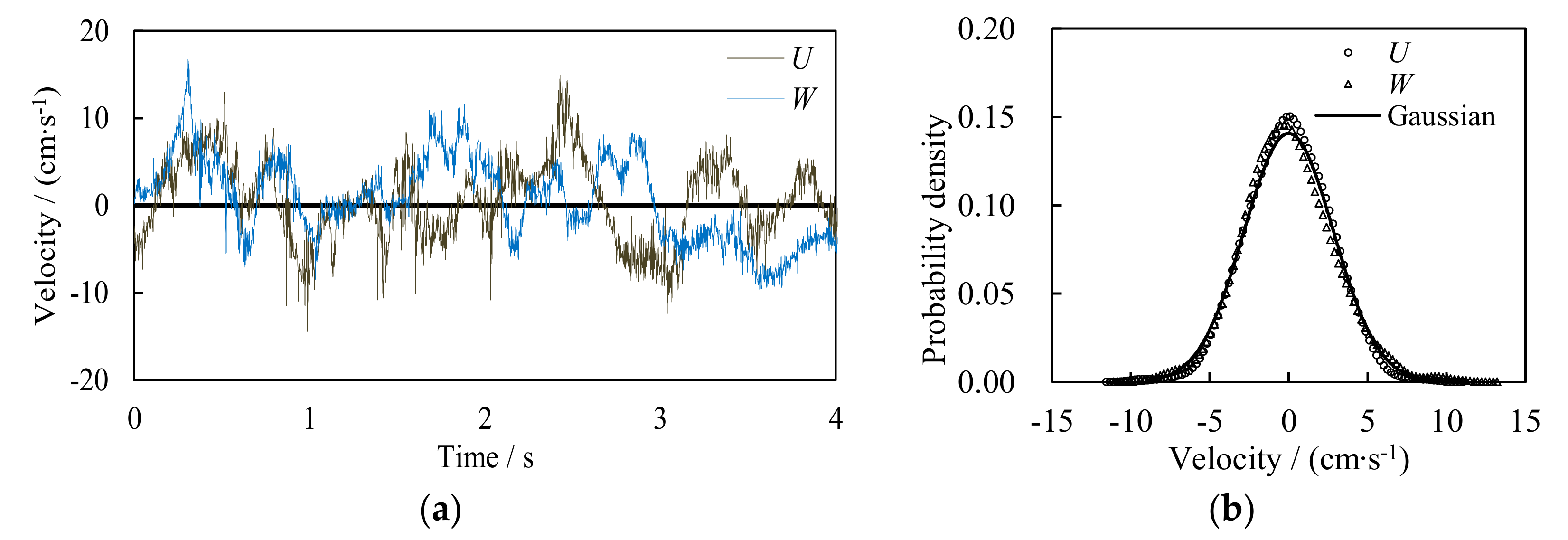
Turbulence is a random process but with statistical regularity, and the velocities of OGT should agree with the Gaussian distribution [3]. The instantaneous flow velocities and their probability density distributions in the middle of the measurement plane are shown in Figure 3. It can be seen that both the longitudinal and vertical velocities are random processes and are well approximated by Gaussian distribution with Skewness and Kurtoses values being 0.1 and 2.42 for U, −0.3 and 2.68 for W, respectively.
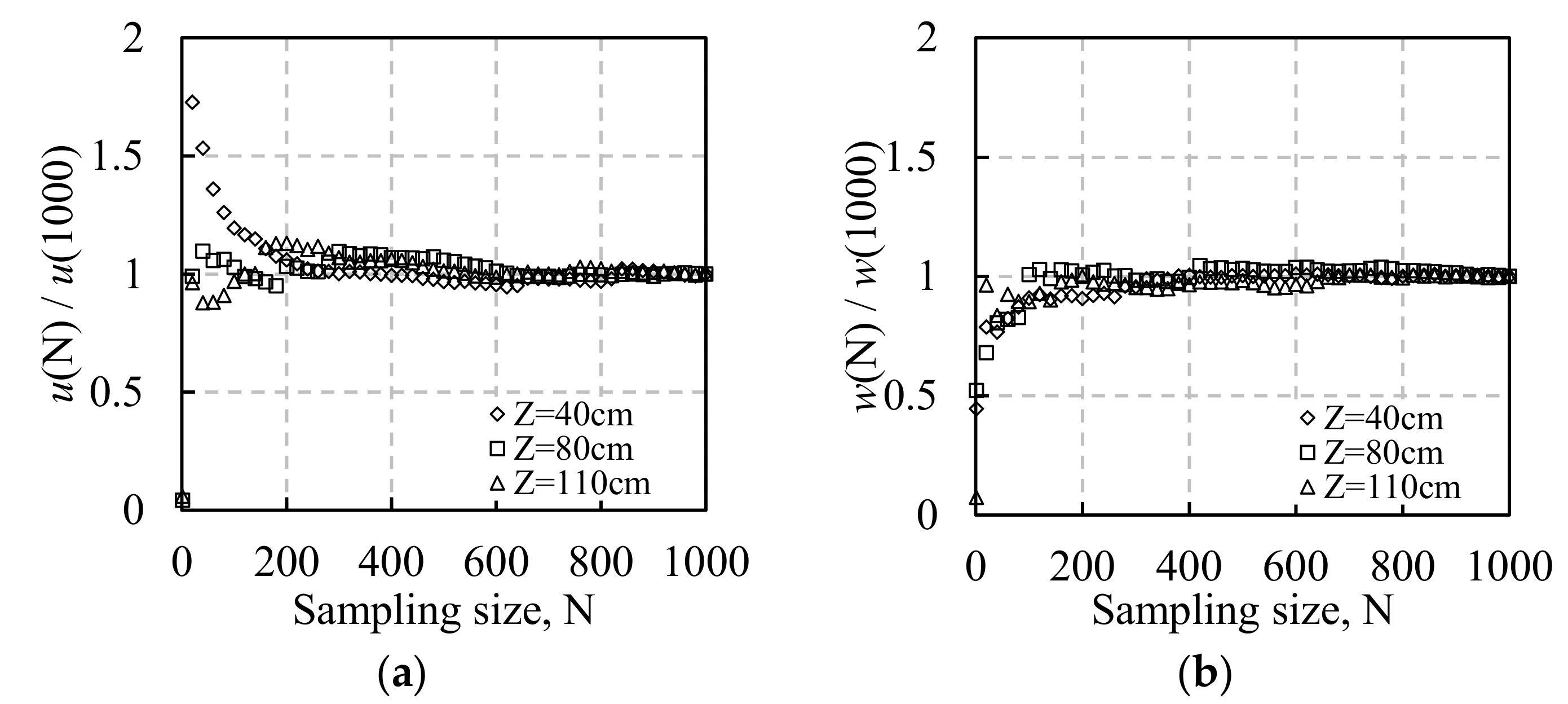
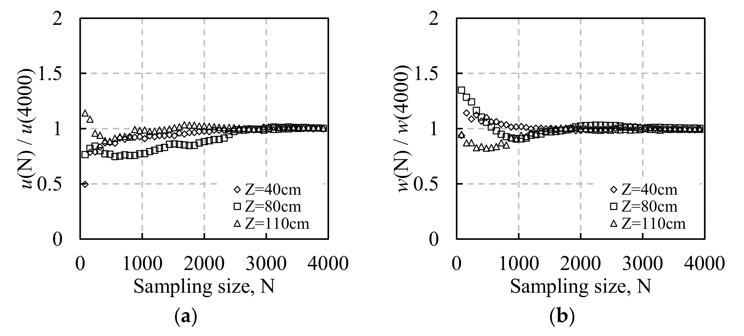
To investigate whether the averaging time is long enough to be able to statistically analyze the flow characteristics, the measurement results of the two sampling methods are examined. The horizontal and vertical RMS velocity fluctuations at three specific elevations are nondimensionalized and presented in Figure 4 and Figure 5.
It clearly illustrates that the statistical results approach a constant when the sampling size exceeds approximately 600 for the sampling frequency of 1.5 Hz, meaning a time duration of 900 s. While the sampling size should be bigger than 3000 for stable statistics when using a sampling frequency of 1000 Hz, meaning a time duration of 3 s. According to the integral time scale and Kolmogorov time scale, which are 2 and 0.28 s, respectively, as calculated in the next section, the duration of a total of 1000 images with frequency of 1.5 Hz covers a 750 integral time scale, ensuring the statistical convergence and thereby the analyses of turbulent intensity level, Reynolds stress and integral scale. With regard to the sampling frequency of 1000 Hz, the duration of a total of 4000 images covers two integral time scale and approximately 15 Kolmogorov time scale, and can also ensure the statistical convergence to analyze the Kolmogorov scale and energy spectra.
3.2. Region of Shear-Free Turbulence
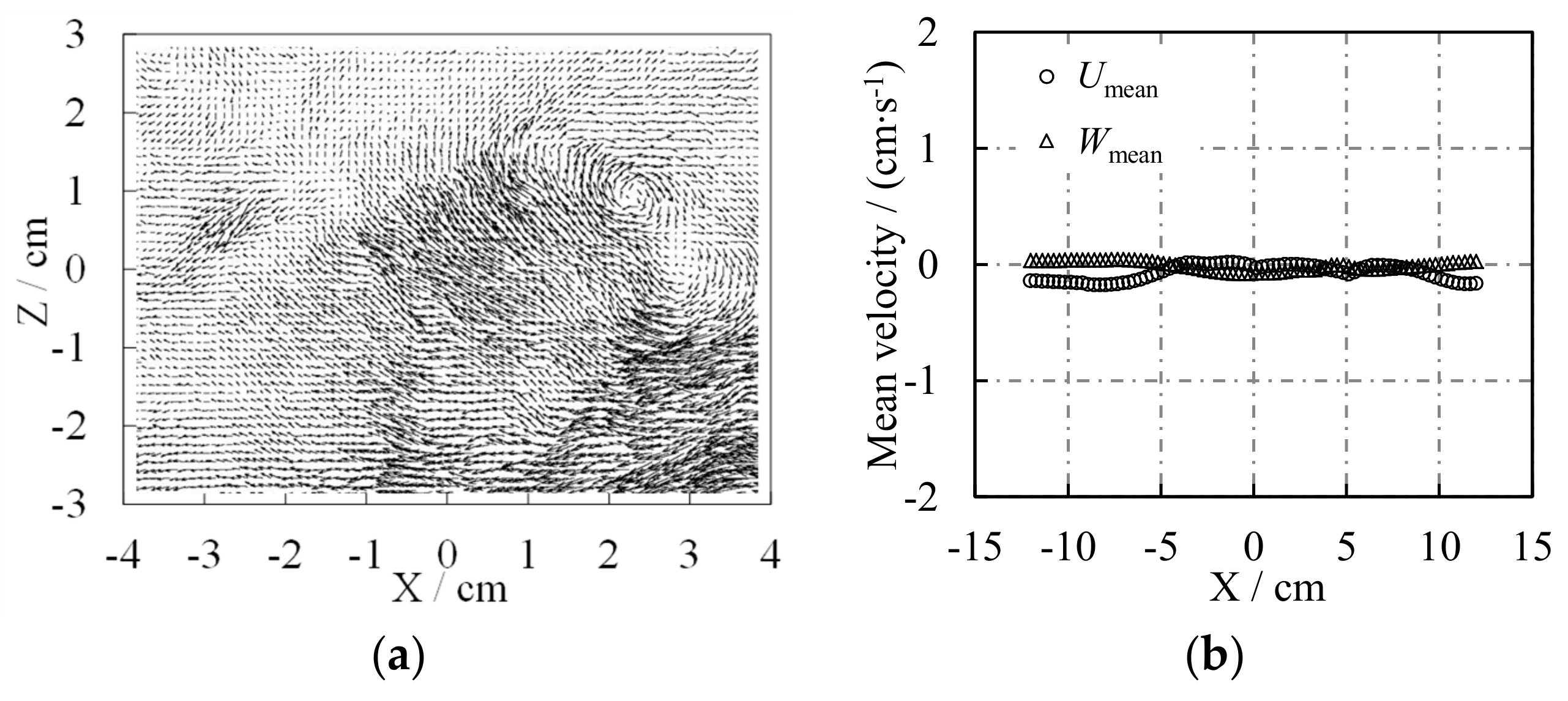
The instantaneous velocity field showing U and W components in the X–Z plane is illustrated in Figure 6a, a large eddy with a size of about 20 mm determining the integral length scale is clearly seen. The spatial distributions of temporally averaged mean velocities Umean and Wmean are shown in Figure 6b. Results indicate that the mean flows are homogeneous and almost zero over the center region of the water tank (−4 cm < X < 4 cm). The mean velocities are negligible compared to the magnitude of the turbulent intensity level.
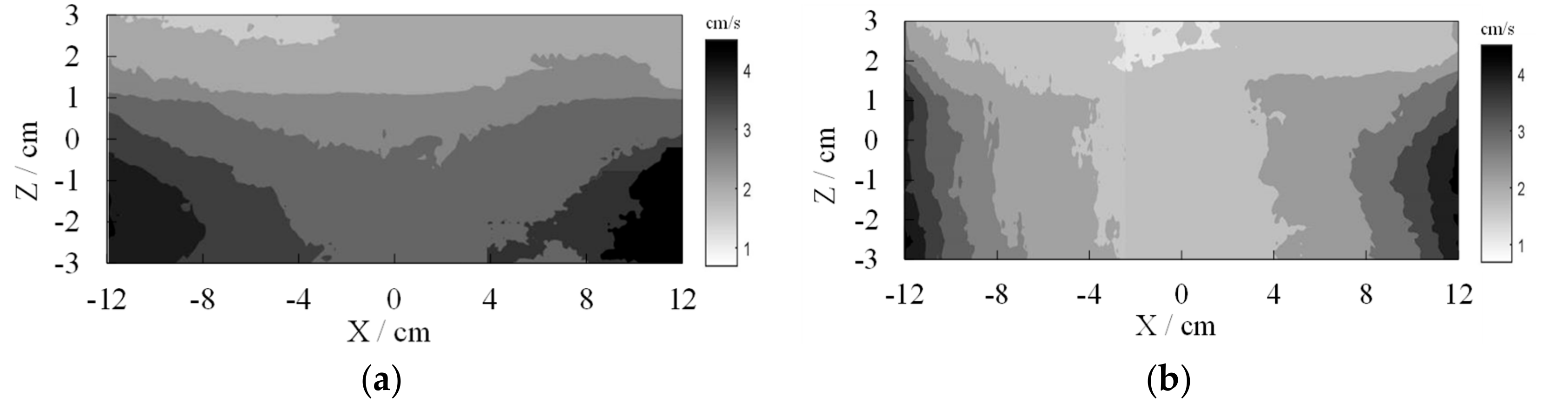
The RMS velocities of two components at zone A2-B2-C2 are shown in Figure 7. Results indicate that the RMS velocities near the grids are relatively big, and decay with the increasing distance from the grid, then become constant near the core region of the water tank (−4 cm < X < 4 cm), consistent with the previous results by using a pair of oscillating girds [7,40].
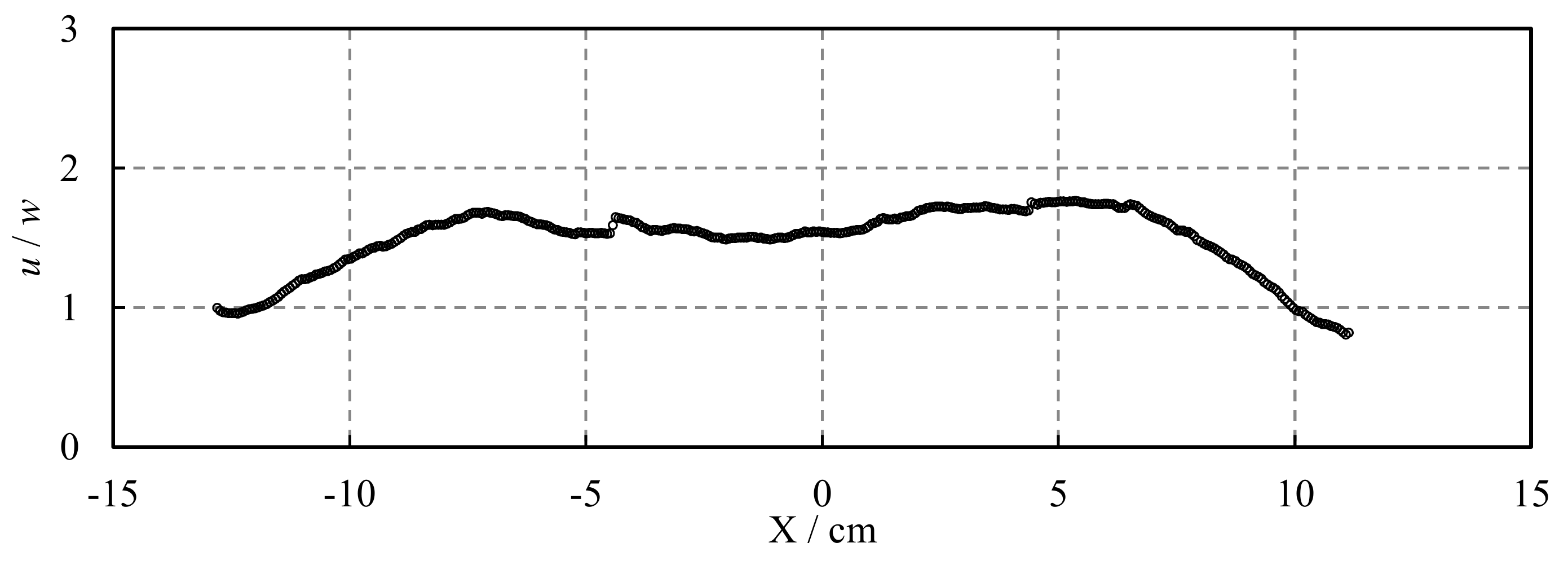
Usually, u was always smaller than w by the vertical oscillating grid in previous studies, and a ratio of u/w being 0.8–0.9 was obtained. Comparatively, the advantage of this study is that a relatively stable ratio of u/w being 1.5–2.0 in the core region (−4 cm < X < 4 cm) is obtained as shown in Figure 8, which agrees with those measured in open-channel flows [42]. The result indicates that the turbulent intensity level in the oscillating direction is always bigger than that in other directions, and the horizontal oscillating grid may be more appropriate when studying the fundamental turbulent mechanisms in open-channel flows.
The spatial distribution of the Reynolds stress (−uw) along the X direction is shown in Figure 9, each vertical line in the figure represents the biggest variation amplitude of Reynolds stress at the Y direction. It can be seen that the Reynolds stresses deviate from zero near the grids and the variations are also relatively big, while the turbulence is nearly shear-free with small variations at the core region of the water tank (−4 cm < X < 4 cm).
The integral length and time scales are calculated as follows:
where fl and ft are spatial and time correlation functions r and τ are space and time intervals and L and T are integral length and time scales. The integral length scale is linearly proportional to the distance from the grid for the oscillating grid turbulence generated by a single grid [37,46]. Using a pair of grids, Srdic et al. (1996) and Shy et al. (1997) found that the integral length scale was almost constant in the central region of the water tank [39,40], while Schulz et al. (2006) suggested a combination of two linear trends for the upper and lower sides between the grids [7]. In this study, both the longitudinal and vertical length scales are first calculated at each distance from the grid, then the total integral length scale L is obtained using the previously used method [7]. Figure 10a shows the distributions of L, indicating that the integral length scale is about 2.4 cm in the core of the two internal grids and decreases away linearly from the core. Additionally, the calculated integral length scale is consistent with the eddy size in Figure 6a. Hannoun (1988) stated that the integral time scale increases linearly with the distance from the grid [3], and Shy et al. (1997) suggested a nearly constant value in the core region [40]. Figure 10b shows the distributions of T, illustrating that the integral time scale is about 2 s in the core of the two internal grids and decreases away from the core. Thus, the integral velocity scale in the core region of the water tank is about 1.2 cm/s, which is consistent with the magnitude of turbulent intensity level.
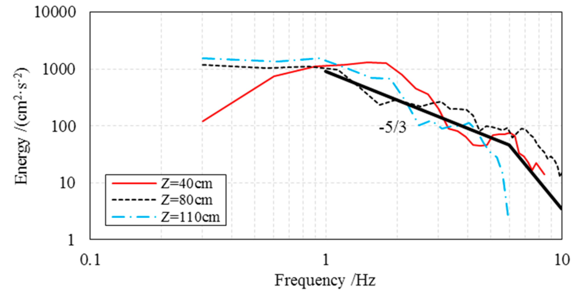
Based on the measurements of the sampling frequency of 1000 Hz, the frequency spectra at the core of the two internal grids are presented in Figure 11. It can be seen that all the frequency spectra in the inertial subrange at different elevations exhibit a slope of −5/3, obeying Kolmogorov’s theory.
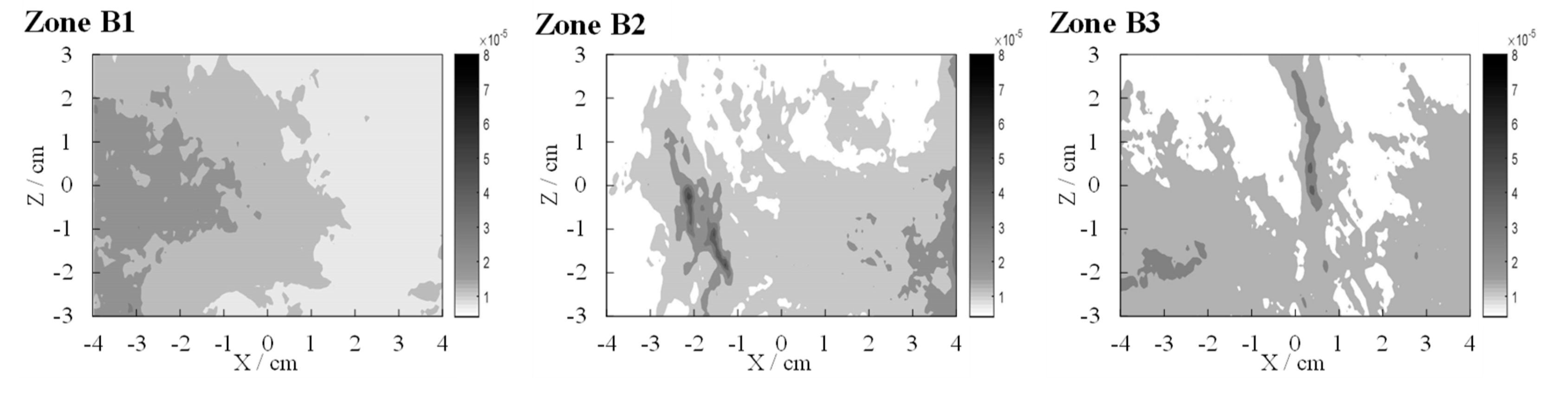
Additionally, the dissipation rate is calculated using [16,18], where ν is the kinematic viscosity and is 1 × 10⁻⁶ m2s−1 for water temperature being about 20 °C in this study. The dissipation rates at different zones are given as shown in Figure 12.
The dissipation rate is mainly between 1 to 2 (10−5 m2s−3), consistent with the range of 10−7 to 10−4 (m2s−3) in the natural flow environments [47]. The averaged dissipation rate of three zones is about 1.27 × 10⁻⁵ m2s−3, which is used to determine the Kolmogorov length scale as η = (ν3/ε)1/4 = 0.53 mm and the Kolmogorov time scale as τ = (ν/ε)1/2 = 0.28 s. The Kolmogorov length scale also agrees with the observed range of 0.4 to 2 mm in natural environments [48]. The values of the integral length scale and Kolmogorov length scale of the proposed apparatus basically span the typical sizes of suspended particles in natural flow environments. According to the Kolmogorov time scale in this study, the dissipation range is reached when the frequency is more than about 4 Hz, and the frequency spectra become steep, as shown in Figure 11.
In summary, a region of shear-free turbulence is generated at the core region of the water tank, probably −4 cm < X < 4 cm, where the mean velocities are homogeneously zero, the ratio of u/w is 1.5–2.0, the turbulent intensity level does not decay, the integral length and time scales are nearly constant and the dissipative range is covered.
3.3. Influence of Stroke and Frequency on Turbulent Intensity Level
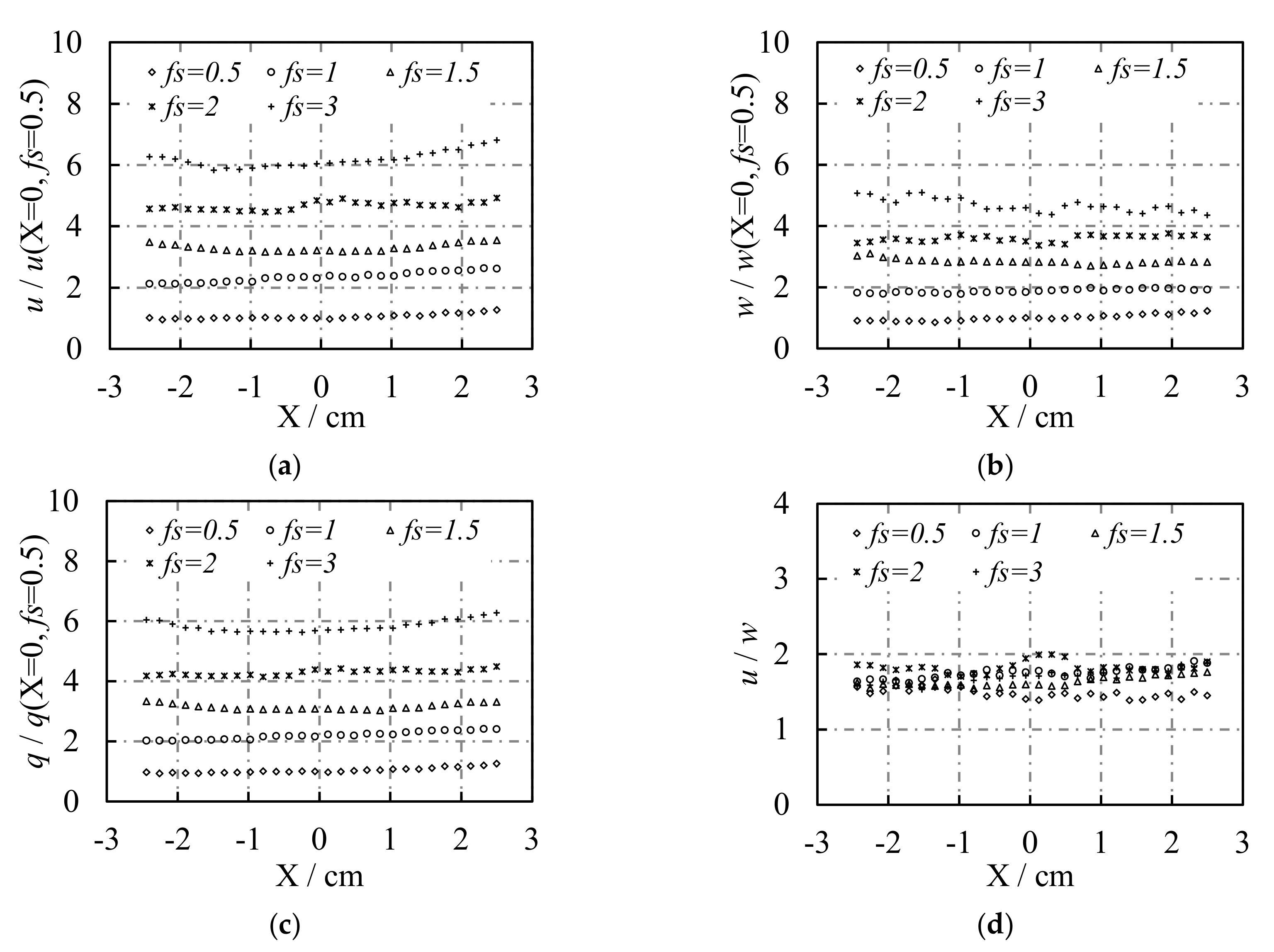
The RMS velocity and RMS of fluctuating velocity under different strokes and frequencies are plotted in Figure 13. It can be seen that the u, w and q are independent of X and increase with the increasing product of stroke and frequency, and u/w is always between 1.5 and 2.0 in the suggested region of shear-free turbulence.
According to Figure 13, the RMS velocity and RMS of fluctuating velocity are linearly proportional to the product of oscillating frequency and oscillating stroke (fs, which has a dimension of cm/s), leading to the following Equation (4) through regression analysis.
Noting that one mesh size is used in the experiments and the mesh size is not included in the above equation.
4. Conclusions
Shear-free turbulence is of extreme interest in studying the turbulence mechanisms and particle–turbulence interactions in open-channel flows. However, the previously used vertical oscillating grids may introduce the inertial influence on vertical migratory behavior, and usually lead to the ratio of u/w being 0.8–0.9, which is approximately 1.5–2.0 yet in open-channel flows. This work employs four horizontal oscillating grids to generate a stationary shear-free turbulent flow field in the center of the water tank, and can be important for turbulence studies. The as-generated turbulence has the following characteristics and advantages:
- (1)
- The time-averaged mean flow velocities are homogeneously zero over the center of the water tank, and are negligible compared to the magnitude of the RMS velocities.
- (2)
- Driven by horizontal oscillation, ratios of u/w being about 1.5–2.0 are obtained in the center of the water tank, consistent with those in open-channel flows, and the turbulent intensity almost does not decay.
- (3)
- The integral length scale and Kolmogorov length scale cover the common sizes of the suspended particles in natural flow environments, and the dissipation rate range also agrees with the values found in natural environments.
- (4)
- The turbulent intensity level presents a linear relationship with the product of oscillating stroke and frequency in the center of the water tank, and a formula is suggested to calculate the RMS velocity for the convenience of practical application.
The proposed horizontal oscillating mode may eliminate the vertical inertial influence, and should be more appropriate for studying the vertical migratory behavior. In terms of the influences of oscillating frequency and stroke, only the turbulent intensity level is investigated, the change of the shear-free region needs further studies and a larger shear-free region is expected to be achieved due to the large water tank in this study.
Author Contributions
Conceptualization, Y.X.; methodology, S.Y.; formal analysis, P.Z.; data curation, X.F.; writing—review and editing, W.L. All authors have read and agreed to the published version of the manuscript.
Funding
This research was funded by National Natural Science Foundation of China, grant number 51679019; National Key Research and Development Program of China, grant number 2018YFB1600400.
Acknowledgments
The authors would like to express the gratitude to Wang Xingkui, Chen Qigang and Zhong Qiang in Tsinghua University for their help in designing the Oscillating grid system and their excellent suggestions, which strengthened this work.
Conflicts of Interest
The authors declare no conflicts of interest.
References
- Mohamed, M.S.; LaRue, J.C. The decay power law in grid-generated turbulence. J. Fluid Mech. 1990, 219, 195–214. [Google Scholar] [CrossRef]
- Hopfinger, E.J.; Toly, J.A. Spatially decaying turbulence and its relation to mixing across density interfaces. J. Fluid Mech. 1976, 78, 155–175. [Google Scholar] [CrossRef]
- Hannoun, I.A.; List, E.J. Turbulent mixing at a shear free density interface. J. Fluid Mech. 1988, 189, 211–234. [Google Scholar] [CrossRef]
- De Silva, I.P.D.; Fernando, H.J.S. Oscillating grids as a source of nearly isotropic turbulence. Phys. Fluids 1994, 6, 2455–2464. [Google Scholar] [CrossRef]
- Orlins, J.J.; Gulliver, J.S. Turbulence quantification and sediment resuspension in an oscillating grid chamber. Exp. Fluids 2003, 34, 662–677. [Google Scholar] [CrossRef]
- Buchholz, J.; Eidelman, A.; Elperin, T.; Grünefeld, G.; Kleeorin, N.; Krein, A.; Rogachevskii, I. Experimental study of turbulent thermal diffusion in oscillating grids turbulence. Exp. Fluids 2004, 36, 879–887. [Google Scholar] [CrossRef]
- Schulz, H.E.; Janzen, J.G.; Souza, K.C.O. Experiments and theory for two grids turbulence. J. Braz. Soc. Mech. Sci. Eng. 2006, 28, 216–223. [Google Scholar] [CrossRef]
- Yan, J.; Cheng, N.S.; Tang, H.W.; Tan, S.K. Oscillating-grid turbulence and its applications: A review. J. Hydraul. Res. 2007, 45, 26–32. [Google Scholar] [CrossRef]
- Pujol, D.; Colomer, J.; Serra, T.; Casamitjana, X. Effect of submerged aquatic vegetation on turbulence induced by an oscillating grid. Cont. Shelf Res. 2010, 30, 1019–1029. [Google Scholar] [CrossRef]
- Traugott, H.; Hayse, T.; Liberzon, A. Resuspension of particles in an oscillating grid turbulent flow using PIV and 3D-PTV. J. Phys. Conf. Ser. 2011, 318, 52021–52030. [Google Scholar]
- Birouk, M.; Sarh, B.; Gökalp, I. An attempt to realize experimental isotropic turbulence at low Reynolds number. Flow Turbul. Combust. 2003, 70, 325–348. [Google Scholar] [CrossRef]
- Hwang, W.; Eaton, J.K. Creating homogeneous and isotropic turbulence without a mean flow. Exp. Fluids 2004, 36, 444–454. [Google Scholar] [CrossRef]
- Warnaars, T.A.; Hondzo, M.; Carper, M.A. A desktop apparatus for studying interactions between microorganisms and small-scale fluid motion. Hydrobiologia 2006, 563, 431–443. [Google Scholar] [CrossRef]
- Voth, G.A.; La Porta, A.; Crawford, A.M.; Alexander, J.; Bodenschatz, E. Measurement of particle accelerations in fully developed turbulence. J. Fluid Mech. 2002, 469, 121–160. [Google Scholar] [CrossRef] [Green Version]
- Variano, E.A.; Bodenschatz, E.; Cowen, E.A. A random synthetic jet array driven turbulence tank. Exp. Fluids 2004, 37, 613–615. [Google Scholar] [CrossRef]
- Webster, D.R.; Brathwaite, A.; Yen, J. A novel laboratory apparatus for simulating isotropic oceanic turbulence at low Reynolds number. Limnol. Oceanogr. Methods 2004, 2, 1–12. [Google Scholar] [CrossRef]
- Krawczynski, J.F.; Renou, B.; Danaila, L. The structure of the velocity field in a confined flow driven by an array of opposed jets. Phys. Fluids 2010, 22, 557–563. [Google Scholar] [CrossRef]
- Bellani, G.; Variano, E.A. Homogeneity and isotropy in a laboratory turbulent flow. Exp. Fluids 2014, 55, 1646. [Google Scholar] [CrossRef] [Green Version]
- Pérez-Alvarado, A.; Mydlarski, L.; Gaskin, S. Effect of the driving algorithm on the turbulence generated by a random jet array. Exp. Fluids 2016, 57, 20. [Google Scholar] [CrossRef]
- Rouse, H. Experiments on the mechanics of sediment suspension. In Proceedings of the 5th International Congress of Applied Mechanics, Cambridge, MA, USA, 12–16 September 1939; pp. 550–554. [Google Scholar]
- Tsai, C.H.; Lick, W. A portable device for measuring sediment resuspension. J. Great Lakes Res. 1986, 12, 314–321. [Google Scholar] [CrossRef]
- Huppert, H.E.; Turner, J.S.; Hallworth, M.A. Sedimentation and entrainment in dense Layers of suspended particles stirred by an oscillating grid. J. Fluid Mech. 1995, 289, 263–293. [Google Scholar] [CrossRef] [Green Version]
- McDougall, T.J. Measurement of turbulence in a zero-mean-shear mixed layer. J. Fluid Mech. 1979, 94, 409–431. [Google Scholar] [CrossRef]
- Brumley, B.H.; Jirka, G.H. Near-surface turbulence in a grid-stirred tank. J. Fluid Mech. 1987, 183, 236–263. [Google Scholar] [CrossRef]
- Chu, C.R.; Jirka, G.H. Turbulent gas flux measurements below the air-water interface of a grid-stirred tank. Int. J. Heat Mass Transfer 1992, 35, 1957–1968. [Google Scholar]
- Connolly, J.P.; Armstrong, N.E.; Miksad, R.W. Adsorption of hydrophobic pollutants in estuaries. J. Environ. Eng. 1983, 109, 17–35. [Google Scholar] [CrossRef]
- Valsaraj, K.T.; Ravikrishna, R.; Orlins, J.J.; Smith, J.S.; Gulliver, J.S.; Reible, D.D.; Thibodeaux, L.J. Sediment-to-air mass transfer of semi-volatile contaminants due to sediment resuspension in water. Adv. Environ. Res. 1997, 1, 145–156. [Google Scholar]
- Ettema, R.; Karim, F.; Kennedy, J.F. Laboratory experiments on frazil ice growth in supercooled water. Cold Reg. Sci. Technol. 1984, 10, 43–58. [Google Scholar] [CrossRef]
- Jirka, G.H. Experiments on gas transfer at the air-water interface induced by oscillating grid turbulence. J. Fluid Mech. 2008, 594, 183–208. [Google Scholar] [CrossRef]
- Buscombe, D.; Conley, D.C. Schmidt number of sand suspensions under oscillating grid turbulence. Coast. Eng. Proc. 2012, 1, 1–11. [Google Scholar] [CrossRef] [Green Version]
- Wan Mohtar, W.H.M.; Zakaria, N.M. The interaction of oscillating-grid turbulence with a sediment layer. Res. J. Appl. Sci. Eng. Technol. 2013, 6, 598–608. [Google Scholar] [CrossRef]
- Laizet, S.; Vassilicos, J.C. Stirring and scalar transfer by grid-generated turbulence in the presence of a mean scalar gradient. J. Fluid Mech. 2015, 764, 52–75. [Google Scholar] [CrossRef] [Green Version]
- Zhou, Y.; Nagata, K.; Sakai, Y.; Ito, Y.; Hayase, T. Enstrophy production and dissipation in developing grid-generated turbulence. Phys. Fluids 2016, 28, 025113. [Google Scholar] [CrossRef]
- Melina, G.; Bruce, P.J.K.; Hewitt, G.F.; Vassilicos, J.C. Heat transfer in production and decay regions of grid-generated turbulence. Int. J. Heat Mass Transfer 2017, 109, 537–554. [Google Scholar] [CrossRef]
- Corrsin, S. Turbulence: Experiment methods. In Handbuch der Physik; Springer: Berlin, Germany, 1963; Volume 8, pp. 524–590. [Google Scholar]
- Thompson, S.M.; Turner, J.S. Mixing across an interface due to turbulence generated by an oscillating grid. J. Fluid Mech. 1975, 67, 349–368. [Google Scholar] [CrossRef]
- Cheng, N.S.; Law, A.W.K. Measurements of turbulence generated by oscillating grid. J. Hydraul. Eng. 2001, 127, 201–208. [Google Scholar] [CrossRef]
- Villermaux, E.; Sixou, B.; Gagne, Y. Intense vertical structures in grid-generated turbulence. Phys. Fluids 1995, 7, 2008–2013. [Google Scholar] [CrossRef] [Green Version]
- Srdic, A.; Fernando, H.J.S.; Montenegro, L. Generation of nearly isotropic turbulence using two oscillating grids. Exp. Fluids 1996, 20, 395–397. [Google Scholar] [CrossRef]
- Shy, S.S.; Tang, C.Y.; Fann, S.Y. Nearly isotropic turbulence generated by a pair of vibrating grid. Exp. Therm. Fluid Sci. 1997, 14, 251–262. [Google Scholar] [CrossRef]
- Ott, S.; Mann, J. An experimental investigation of the relative diffusion of particle pairs in three-dimensional turbulent flow. J. Fluid Mech. 2000, 422, 207–223. [Google Scholar] [CrossRef]
- Nezu, I.; Rodi, W. Open channel flow measurements with a Laser Doppler Anemometer. J. Hydraul. Eng. 1986, 112, 335–355. [Google Scholar] [CrossRef]
- Franks, P.J.S. Turbulence avoidance: An alternate explanation of turbulence-enhanced ingestion rates in the field. Limnol. Oceanogr. 2001, 46, 959–963. [Google Scholar] [CrossRef]
- Incze, L.S.; Hebert, D.; Wolff, N.; Oakey, N.; Dye, D. Changes in copepod distributions associated with increased turbulence from wind stress. Mar. Ecol. Prog. 2001, 213, 229–240. [Google Scholar] [CrossRef]
- McKenna, S.P.; McGillis, W.R. Observations of flow repeatability and secondary circulation in an oscillating grid-stirred tank. Phys. Fluids 2004, 16, 3499–3502. [Google Scholar] [CrossRef]
- Liu, C.R.; Huhe, A.D. Homogeneous turbulence structure near the wall and sediment incipience. Ocean Eng. 2003, 21, 50–55. [Google Scholar]
- Granata, T.C.; Dickey, T.D. The fluid-mechanics of copepod feeding in a turbulent flow: A theoretical approach. Prog. Oceanogr. 1991, 26, 243–261. [Google Scholar] [CrossRef]
- Jiménez, J. Oceanic turbulence at millimeter scales. Sci. Mar. 1997, 61, 47–56. [Google Scholar]
Figure 1.
Sketch map of the experimental system.

Figure 2.
Plan view of the imaged locations.

Figure 3.
Measured flow velocity of one point: (a) instantaneous velocity; (b) probability density.

Figure 4.
Variation of the RMS velocity with the sampling size when the sampling frequency is 1.5 Hz: (a) RMS velocity in the X direction; (b) RMS velocity in the Z direction.
Figure 4.
Variation of the RMS velocity with the sampling size when the sampling frequency is 1.5 Hz: (a) RMS velocity in the X direction; (b) RMS velocity in the Z direction.

Figure 5.
Variation of the RMS velocity with the sampling size when the sampling frequency is 1000 Hz: (a) RMS velocity in the X direction; (b) RMS velocity in the Z direction.
Figure 5.
Variation of the RMS velocity with the sampling size when the sampling frequency is 1000 Hz: (a) RMS velocity in the X direction; (b) RMS velocity in the Z direction.

Figure 6.
Distribution of the measured flow velocity when s = 0.5 cm and f = 3 Hz: (a) instantaneous velocity field of zone B2; (b) mean velocity along the X direction.
Figure 6.
Distribution of the measured flow velocity when s = 0.5 cm and f = 3 Hz: (a) instantaneous velocity field of zone B2; (b) mean velocity along the X direction.

Figure 7.
The RMS velocity when s = 0.5 cm and f = 3 Hz: (a) u component; (b) w component.

Figure 8.
Variation of the ratio of u/w along the X direction when s = 0.5 cm and f = 3 Hz.

Figure 9.
The spatial distribution of Reynolds stress and the variations when s = 0.5 cm and f = 3 Hz.
Figure 9.
The spatial distribution of Reynolds stress and the variations when s = 0.5 cm and f = 3 Hz.

Figure 10.
Spatial distribution of the integral scale at different X position when s = 0.5 cm and f = 3 Hz: (a) integral length scale; (b) integral time scale.
Figure 10.
Spatial distribution of the integral scale at different X position when s = 0.5 cm and f = 3 Hz: (a) integral length scale; (b) integral time scale.

Figure 11.
Frequency spectra at different elevations when s = 0.5 cm and f = 3 Hz.

Figure 12.
Dissipation rate contours at different zones when s = 0.5 cm and f = 3 Hz.

Figure 13.
Turbulent intensity level (nondimensionalized using their reference values at X = 0, fs = 0.5 cm/s) under different strokes and frequencies: (a) u component; (b) w component; (c) q; (d) u/w.
Figure 13.
Turbulent intensity level (nondimensionalized using their reference values at X = 0, fs = 0.5 cm/s) under different strokes and frequencies: (a) u component; (b) w component; (c) q; (d) u/w.


Table 1.
Experimental details of oscillating grid turbulence (OGT) in the previous studies.
| Researchers | Tank Length (cm) | Tank Width (cm) | Tank Height (cm) | Grid Mesh Size (cm) | Oscillating Frequency (Hz) | Oscillating Stroke (cm) | Measurement Technique 1 |
|---|---|---|---|---|---|---|---|
| Hopfinger and Toly [2] | 67.5 | 67.5 | 100 | 5, 10 | 2–6 | 4, 8, 9 | Hot-film |
| Hannoun et al. [3] | 115 | 115 | 335 | 6.35 | 2.25 | 6.35 | LDV |
| De Silva and Fernando [4] | 26 | 26 | 60 | 2.9, 4.7, 6.2 | 1–5 | 0.85, 2.1 | LDV |
| Cheng and Law [37] | 50 | 50 | 100 | 5 | 1–4 | 4 | PIV |
| Orlins and Gulliver [5] | 50 | 50 | 50 | 8 | 3, 5, 7 | 3 | LDV |
| Schulz et al. [7] | 50 | 50 | 115 | 5.1 | 1–4 | 2–5 | PIV |
| Buscombe and Conley [30] | 50 | 50 | 80 | 5 | 2, 3 | 7, 10 | ADV |
| Wan Mohtar et al. [31] | 35.4 | 35.4 | 50 | 5 | 3 | 8 | PIV |
| Present study | 100 | 100 | 200 | 10 | 1, 2, 3 | 0.5, 1, 1.5 | PIV |
1 LDV = Laser Doppler Velocimetry; ADV = Acoustic Doppler Velocimeter; PIV = Particle Image Velocimetry.
Table 2.
Experimental set-up used to conduct the measurements.
| Measured Zone | Oscillating Stroke (cm) | Oscillating Frequency (Hz) | Sampling Frequency (Hz) | Duration (s) |
|---|---|---|---|---|
| A1, A2, A3, B1, B2, B3, C1, C2, C3 | 0.5 | 3 | 1.5, 1000 | 1500, 4 |
| B2 | 0.5 | 2 | 1.5 | 1500 |
| 0.5 | 1 | |||
| 1 | 3 | |||
| 1 | 2 | |||
| 1 | 1 | |||
| 1.5 | 2 | |||
| 1.5 | 1 |
© 2020 by the authors. Licensee MDPI, Basel, Switzerland. This article is an open access article distributed under the terms and conditions of the Creative Commons Attribution (CC BY) license (http://creativecommons.org/licenses/by/4.0/).
Share and Cite
MDPI and ACS Style
Li, W.; Zhang, P.; Yang, S.; Fu, X.; Xiao, Y. An Experimental Method for Generating Shear-Free Turbulence Using Horizontal Oscillating Grids. Water 2020, 12, 591. https://doi.org/10.3390/w12020591
AMA Style
Li W, Zhang P, Yang S, Fu X, Xiao Y. An Experimental Method for Generating Shear-Free Turbulence Using Horizontal Oscillating Grids. Water. 2020; 12(2):591. https://doi.org/10.3390/w12020591
Chicago/Turabian StyleLi, Wenjie, Peng Zhang, Shengfa Yang, Xuhui Fu, and Yi Xiao. 2020. "An Experimental Method for Generating Shear-Free Turbulence Using Horizontal Oscillating Grids" Water 12, no. 2: 591. https://doi.org/10.3390/w12020591
Note that from the first issue of 2016, this journal uses article numbers instead of page numbers. See further details here.