Study on Backwater Effect Due to Polavaram Dam Project under Different Return Periods


1
Research Scholar, Department of Civil Engineering, Indian Institute of Technology Hyderabad, Kandi, Telangana 502285, India
2
Faculty, Department of Civil Engineering, Indian Institute of Technology Hyderabad, Kandi, Telangana 502285, India
*
Author to whom correspondence should be addressed.
Water 2020, 12(2), 576; https://doi.org/10.3390/w12020576
Submission received: 29 December 2019
/
Revised: 12 February 2020
/
Accepted: 18 February 2020
/
Published: 20 February 2020
(This article belongs to the Section Hydraulics and Hydrodynamics)
Abstract
:In this study, we present a scenario to evaluate the backwater impacts on upstream of the Polavaram dam during floods. For this purpose, annual peak discharges across the different gauge stations in river stretch considered for flood frequency analysis. Statistical analysis is carried out for discharge data to estimate probable flood discharge values for 1000 and 10,000 years return period along with 0.1 and 0.14 million m3/s discharge. Furthermore, the resulting flood discharge values are converted to water level forecasts using a steady and unsteady flow hydraulic model, such as HEC-RAS. The water surface elevation at Bhadrachalam river stations with and without dam was estimated for 1000 and 10,000 years discharge. Unsteady 2D flow simulations with and without the dam with full closure and partial closure modes of gate operation were analysed. The results showed that with half of the gates as open and all gates closed, water surface elevation of 62.34 m and 72.34 m was obtained at Bhadrachalam for 1000 and 10,000 years. The 2D unsteady flow simulations revealed that at improper gate operations, even with a flow of 0.1 million m3/s, water levels at Bhadrachalam town will be high enough to submerge built-up areas and nearby villages.
1. Introduction
The extreme-flood analysis of upstream areas induced by a downstream dam, especially in a large river has been an interesting topic for many years. The standing-water in downstream of a dam can influence the upstream of the river, by causing the water surface elevation (WSE) to back up towards the upstream. This phenomenon can increase the depth of the river gradually upstream to form a smooth transition between a quasi-normal flow and standing water, forcing an alteration of the hydraulic conditions. The upstream of the river affected by this response would exceed several hundreds of kilometers in low slope rivers, which is termed as the backwater zone [1]. Dams act as a block on rivers and by forming backwater conditions, which in turn affect the water surface profile at upstream of the river [2,3,4,5,6]. There have been numerous studies on dams that these hydraulic structures can limit discharge and elevate water level at the upstream by creating backwater [7,8]. It is a matter of the fact that the backwater effect can induce upstream flooding, depending on the river, geometry, and on the flow and floodplain characteristics [9]. The backwater from downstream to upstream has caused most of the flood disasters. The consequences of flooding by backwater are mainly caused by the faulty design and operations of a large dam. The backwater phenomenon leads to an increase in the water surface level of upstream regions, thereby imposing the threat of submergence during flood events and affecting the longitudinal extent of the river reach. In our present study, we evaluate the area of upstream submergence with and without the construction of a dam along with a combination of gate openings. In producing flood inundation maps, 1-D models are still very popular due to their reduced computational time, their ease of implementation and the reduced need for topographic data when compared to 2-D and 3-D models [10,11]. However, recent studies have found a 1-D approach neglects the transversal variation of hydrodynamic variables, especially in wide floodplains, which can have great importance. 1-D flood models simulate flows that are assumed to be in a longitudinal direction, such as rivers and confined channels. These models are computationally efficient but are subjected to modeling limitations, such as the inability to simulate flood wave lateral diffusion, the subjectivity of cross-section location and orientation, and the discretisation of topography as cross-sections rather than as a continuous surface [12]. Moreover, the applicability of the 2D unsteady hydraulic model has been proved successful in understanding the backwater profile [6,9,13,14].
The modeling software HEC-RAS handles the 2D hydraulic complexity through numerical solutions. For each time step in the 2D unsteady simulation, diffusion wave or full hydrodynamic equations (Shallow-water equations) are solved for each grid cell, ensuring continuity of the flow at all stages of river stretch [15]. The maximum flood so far estimated at Dowleswaram occurred on the 15 of August, 1986 is 0.09 million m3/s. The computed maximum flood for a 500 year return period works out to 0.10 million m3/s [16]. The highest flood level (HFL) of 18.36 m was observed in Dowleswaram on 16 August 1986. Similarly, on 16 August 1986 HFL was observed in Polavaram (28.01 m), Kunavaram (51.3 m), Dummugudem (60.25 m), and Bhadrachalam (55.66 m) [17].
Considering the effects of climate change, irregular and high intense rainfall maximum flood flow in Indian peninsular rivers, Krishna and Godavari would certainly increase in the future. The flooding of the Krishna river occurred during 2009 is reported to be 0.07 million m3/s which were nearly 2.5 times the peak flood of 0.03 million m3/s ever occurred in the last 100 years [18]. The peak flood flow ever occurred in river Godavari in the last 100 years, was 0.09 million m3/s and the Polavaram Dam was designed for 0.10 million m3/s. The Central Water Commission (CWC) had determined the Possible Maximum Flood (PMF) as 0.14 million m3/s, and the dam spillway was redesigned accordingly. If the same phenomenon of Krishna river occurs in the Godavari river, the flood flow would be 0.23 million m3/s which results in a major catastrophe. In the Polavaram project number of villages coming under submergence rose to 371 from 276 as per the latest figures of the project authority for revised Rehabilitation and Resettlement (R&R) (May 2017). As per the records of the R&R Commissioner, the number of project affected families was around 105,601 [19]. It is important to understand the impact and threat to Bhadrachalam town, the effect on heavy water plants, coal mines and on vital resources, due to the construction of Polavaram dam and upstream submergence.
The construction of the Polavaram project has been the focus of study under social, economic, political and environmental aspects from the past seven decades. Its impact has been spreading over three states which were chosen for the analysis as it not only affects villages but also has serious implications to forest and environment [20]. Polavaram dam project may result in the submergence of over 97,000 acres of irrigation land [21]. The case study of Polavaram project has been taken up by several local, national as well as international media and journals. Fieldwork conducted in the area to be affected by the Polavaram project analyzed possible flaws in the resettlement policies from an economic perspective [22]. Several researchers have conducted a detailed survey of the project-affected areas and estimated the number of impacted people would be about 400,000 after adjusting population growth in the past decade [23]. These publications provide detailed information regarding the implementation and question its technical feasibility and use, as well as its impact and consequences [24].
The objective of this study is to compute the backwater levels of the Polavaram dam and its backwater effect on the Bhadrachalam town and upstream areas. The scope of the research includes 1. Computation of maximum design flood for once in 1000 years and 10,000 years for observed maximum discharge considering successive floods. 2. Computation of backwater levels with and without the Polavaram dam with 1000 years and 10,000 years flood discharges and 3. Estimate the extent of a backwater for 0.1 and 0.14 million m3/s floods as per Bureau of Indian Standards (BIS) criteria and Godavari Water Dispute Tribunal (GWDT) Award [25].
2. Study Area
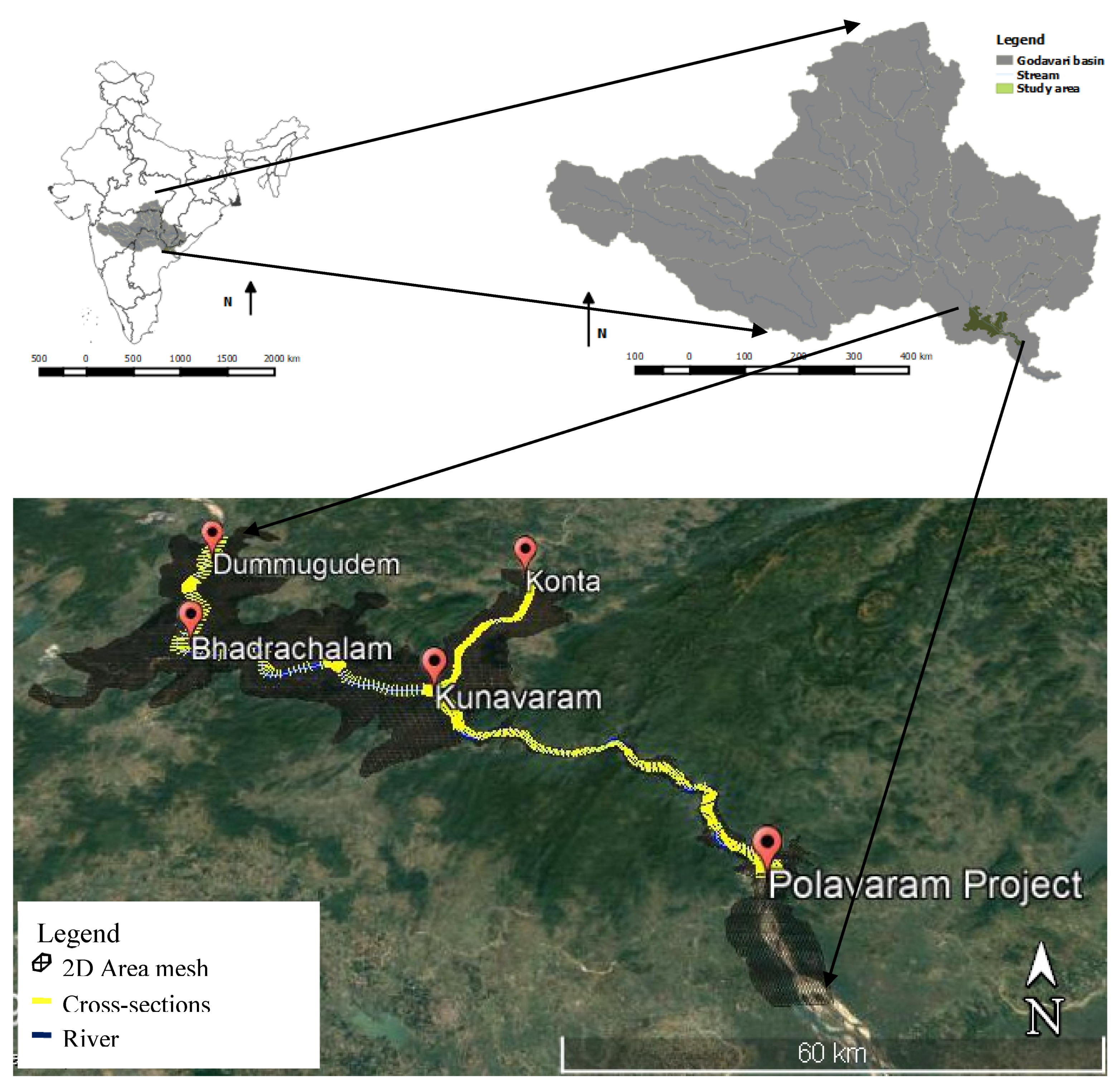
The study domain lies on the main Godavari river stretch, as shown in Figure 1. It covers a distance of around 136 km from Polavaram to Dummugudem along river stretch. Bhadrachalam is located at a distance of around 118 km from the Polavaram dam site. In the study area, two major streams from the upstream (Godavari and Sabari river) meeting at Kunnavaram, forming a junction. Konta is located on Sabari River, which is one of the main tributaries of Godavari River, and it joins the Godavari at Kunnavaram which is around 35 km from Polavaram site.
The Polavaram dam project is located in Andhra Pradesh near Polavaram village about 34 km upstream of Kovvur—Rajahmundry Road and 42 km upstream of Sir Arthur Cotton Barrage, at Longitude 81°39′46″ E and Latitude 17°16′53″ N. It is being built on the Godavari river, the Godavari rising as it does in the heavy rainfall region of the Western Ghats comes under the influence of South-Western monsoon. The region has marked zones with rainfall ranging from 889 mm to 1016 mm. The greater portion of the area drained by the Godavari River receives much more rain during the South-West Monsoon (June to September) than in the North-East Monsoon, and consequently, the river brings down most of its waters between June and September.
It envisages the construction of 2454 m long Earth-cum-rock fill dam across the main river with a spillway of 1128.40 m length on the right flank and power cum river sluices block on the left flank. The dam would comprise 44 gates, with each gate being 16 m width and 20 m in height. It is designed to have a live storage capacity of 23,761 m3/s (75.20 TMC) provided between the full reservoir level (FRL) of 45.72 m and the minimum drawdown level of 41.15 m enabling irrigation of 2.32 million acres. The main intention to begin this project is to divert and utilise the Godavari water to Krishna and other rivers.
The Polavaram FRL is supposed to be maintained at 45.72 m, which is the major take away, among other things by the award of the GWDT [25]. Over 371 villages spread over many mandals in the agency areas of Khammam, East and West Godavari districts along with ten villages in Chhattisgarh, and seven villages in Odisha would possible be submerged under the reservoir [20].
3. Materials and Methods
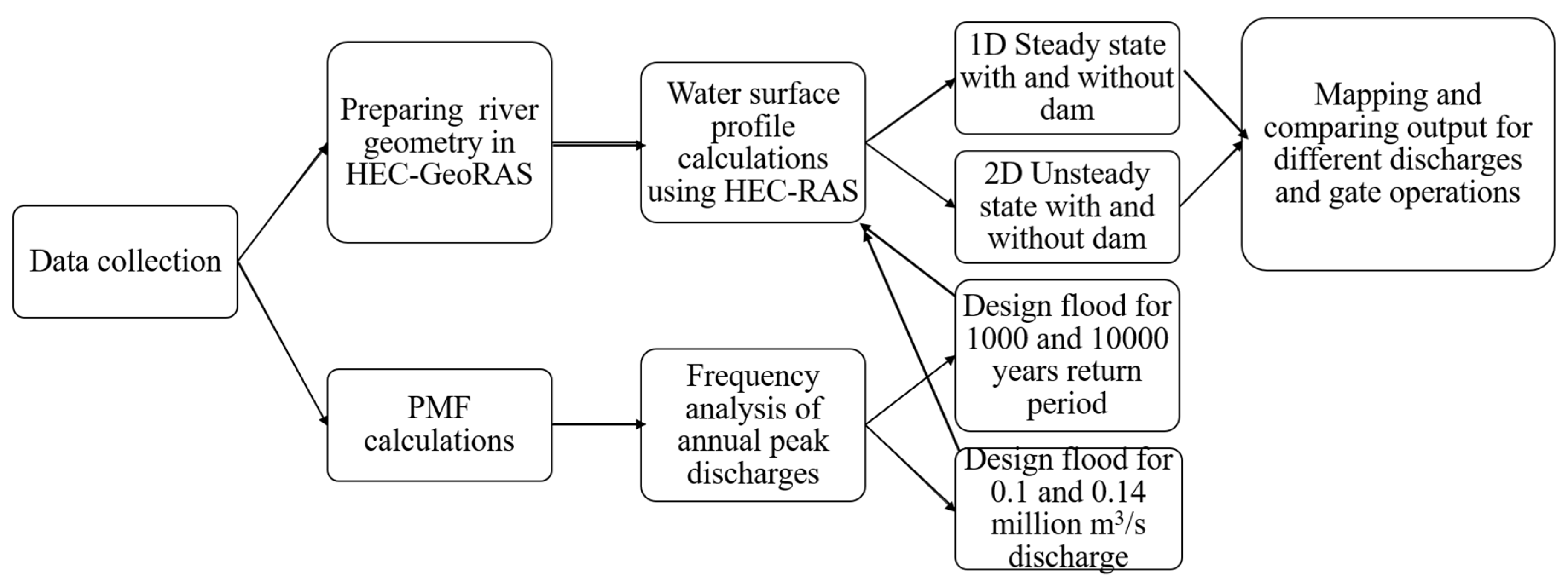
The methodology adopted for this study is shown in Figure 2. This flowchart represents the procedure for flood backwater induced calculations. The Central Water Commission (CWC) has said it has no specific "principles or guidelines" for conducting a study on the assessment of backwater flooding of dams and hydroelectric projects in the country [26]. However, few studies considering the impact of hydraulic structure on upstream areas have followed a similar approach to come up with WSE for different flood discharges.
The probability mass functions were calculated for the collected peak discharge data. HEC-GeoRAS in Geographic information system (Arc-GIS) platform was used; 1. To prepare geometry of the river by including cross-sections, 2. Identifying left and right banks of rivers, 3. Preparing boundary conditions. River geometry was prepared using HEC-GeoRAS, as shown in Figure 1.
Further Probable Maximum Flood (PMF) and Flood frequency analysis were carried out for 0.1 million and 0.14 million m3/s along with a return period of 1,000 and 10,000 years flood. These discharge values were used to simulate water surface elevations at the desired location.
3.1. Data Collection
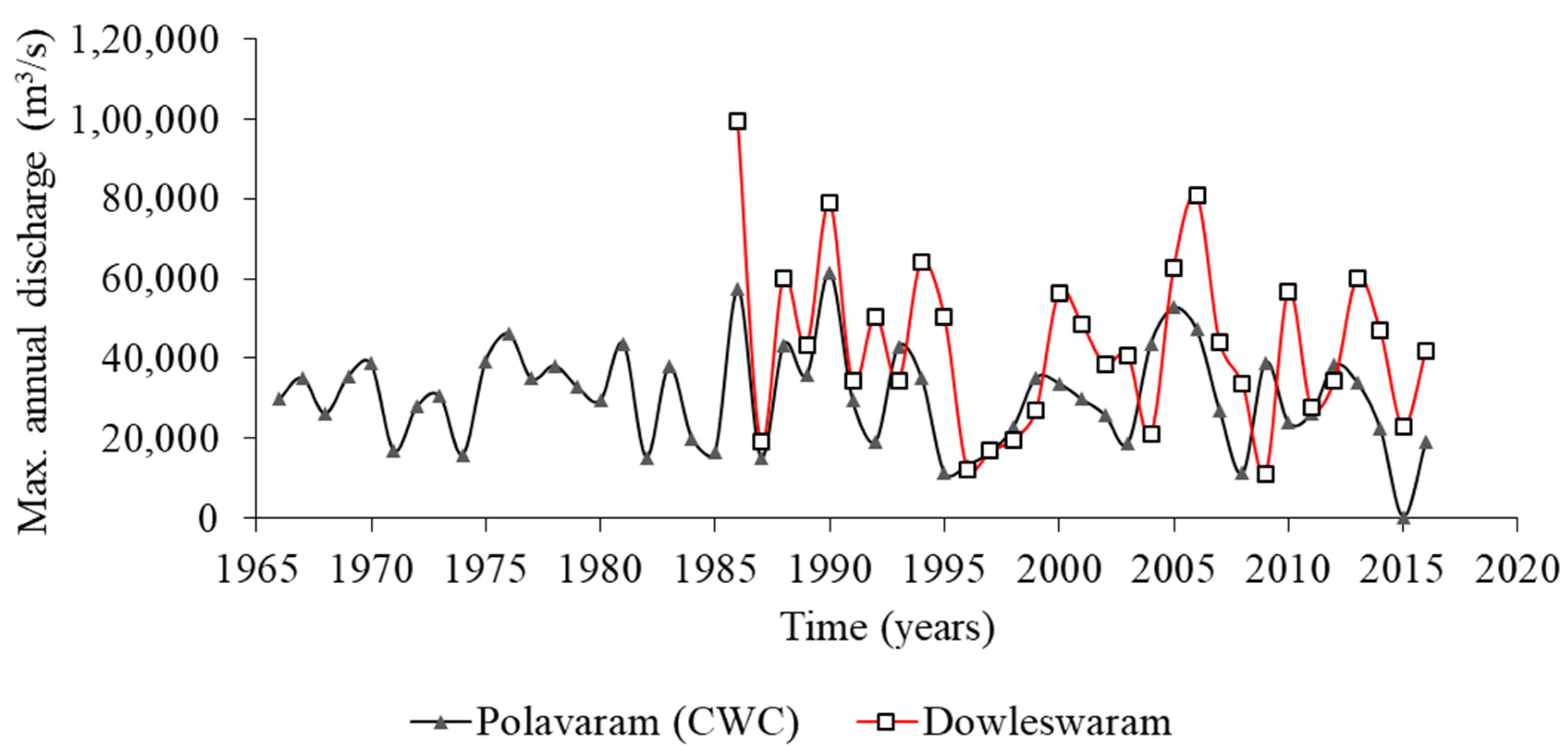
Details of data collected along with sources are mentioned in Table 1. Data about daily discharge in the river obtained from different sources: One at Polavaram (CWC) and another at Dowleswaram (a downstream distance of 38 km from Polavaram). The geometry of the study area prepared using Hec-GeoRas (ArcGIS interface) using digital elevation model (DEM), shapefile of river stretch, and Cross-section data across the river stretch. DEM collected from the USGS website (https://earthexplorer.usgs.go) with a resolution of 30 m. Left and right banks of river stretch were demarcated manually. Annual maximum discharges from both locations were considered for analysis. The maximum annual discharge values data collected from Polavaram and Dowleswaram, as shown in Figure 3.
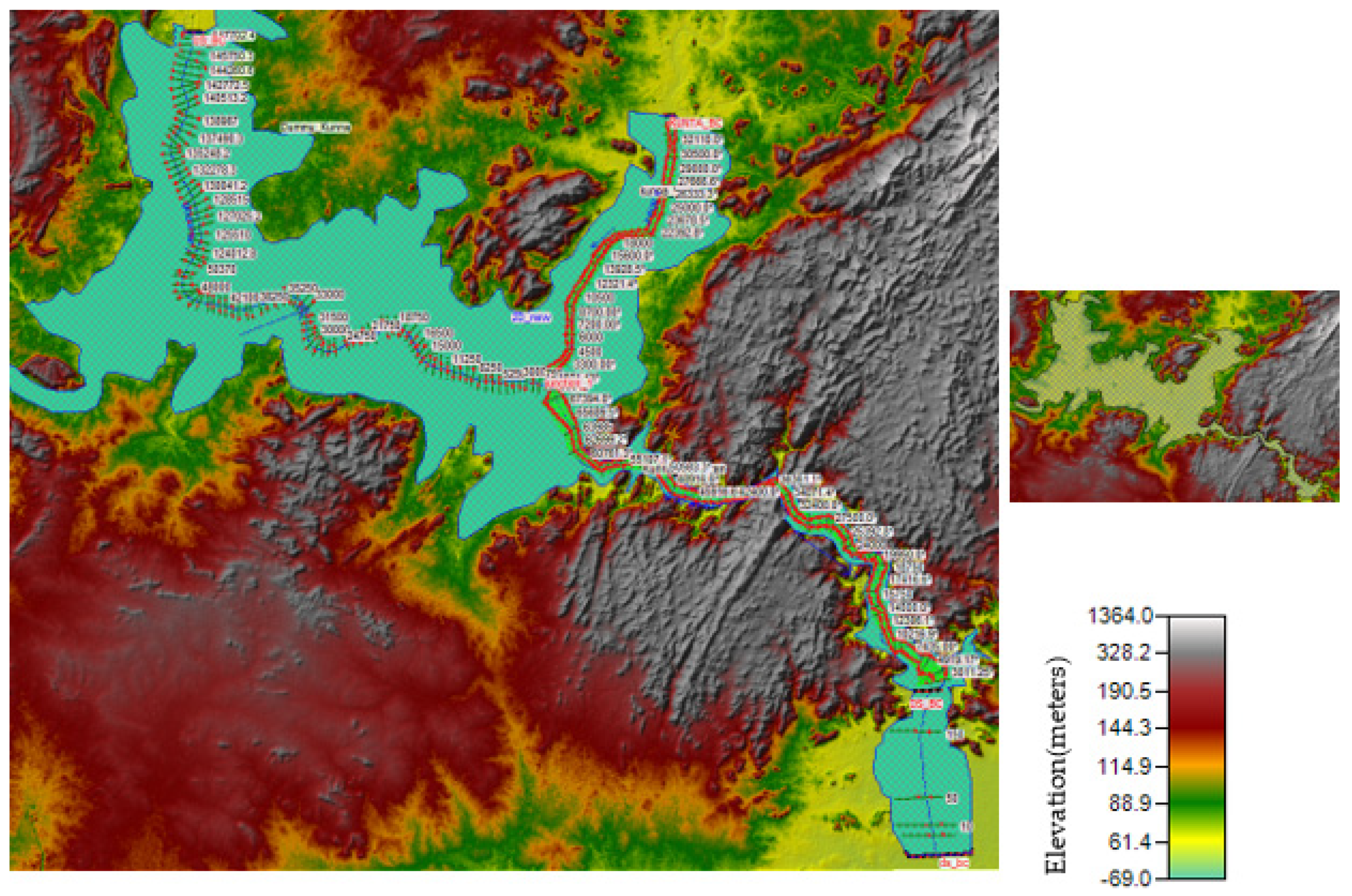
The HEC-GeoRAS is used to describe the river channel and the surrounding floodplains as a series of extended cross-sections perpendicular to the flow direction. HEC-GeoRAS is an extension for ArcGIS® software. ArcGIS®, with the 3D Analyst and Spatial Analyst extensions, are required to use HEC-GeoRAS. The channel and the floodplain geometry were created in the ArcGIS environment, with existing DEM, stream centerline, the bank lines, the flow path centerlines, and the cross-section cut lines. Further, a RAS GIS import file was generated based on the defined geometric characteristics, which was used as an input file, in the Geometric Data Editor of the HEC-RAS model. The DEM was derived using a Shuttle Radar Topography Mission (SRTM) of 30 m × 30 m resolution, as shown in Figure 4.
Field surveyed cross-section data were obtained from local government departments at various locations, as shown in Table 1. The minimum interval of data was 750 m and distributed unevenly. As the model suggested, it was necessary to supplement surveyed cross-section data by interpolating between two surveyed sections. Interpolation of the cross-section was done for 25 m for the present study area. It was decided based on the availability of cross-sections at critical locations and stability of the model. The interpolation routines are not restricted to a set number of master cords. At a minimum, there must be two master cords, but there is no maximum. The interpolation routines will also interpolate roughness coefficients (Manning’s n). In addition to Manning’s n values, the following information is interpolated automatically for each generated cross-section: downstream reach lengths; main channel bank stations; contraction and expansion coefficients; normal ineffective flow areas; levees; and normal blocked obstructions [27]. The cross-sections were further extended on both sides of the river channel to represent the floodplain topography. Figure 4 shows the number of cross-sections considered for the study along with river banks and DEM used.
3.2. Estimation of Probabilistic Floods
Probabilistic flood estimation is used to estimate the flood discharge, which has a particular probability of occurrence, using records for the site in question. Normally the approaches assume that the observations are representative of the long-term behavior of the river system, that there is no trend in the frequency of occurrence, and that the future flooding probabilities can thus be assessed from a frequency analysis of the past regime. In the context of large scale environmental and climate change, all assumptions can be open to challenge [15]. Probability assessment was used to determine the design for floods corresponding to Dam, where it is usually done for 1% (100-year) flood or the 0.1% (1000 years) flood or 0.01% (10,000 years) etc.
3.3. Parameter Estimation for Different Distributions
The probability distribution functions normal, lognormal, gamma (2P), Weibull (2P), Pearson (5 and 6), log Pearson 3 and generalized extreme value were identified to evaluate the best fit probability distribution for annual discharge. The chi-square test at a (0.05) was used to analyze the goodness of fit. The test statistic of each test was computed and tested at (α = 0.05) level of significance. Accordingly, the ranking of different probability distributions was marked from 1 to 8 based on the minimum test statistic value. The distribution holding the first rank (normal) was selected for the calculation of water surface elevation.
3.4. HEC-RAS Model
The HEC-RAS model consists of 1-D components of river analysis to 1. Calculate the water surface profile in a steady flow, 2. Stimulate the unsteady flow (one-dimensional and two-dimensional hydrodynamics [27]. The main element is that the components use a common representation of geometric data and common routines for geometric and hydraulic calculations [28]. In the present project, we used Steady and Unsteady flow water surface profile calculations, combined 1D and 2D hydrodynamics and spatial mapping of computed parameters like depth, water surface elevation, and velocity.
3.4.1. Steady Flow Water Surface Profiles
Gradually varied steady flows can handle a single river reach, a dendritic system, or a full network of channels. The steady flow model has the capability of modeling subcritical, supercritical, and mixed flow regime-water surface profiles. The basic computational procedure is based on the solution of the one-dimensional energy equation (Equation (1)). Energy losses are evaluated by friction (Manning’s equation) and contraction/expansion (coefficient multiplied by the change in velocity head). The momentum equation is utilized in situations where the water surface profile is rapidly varied. These situations include mixed flow regime calculations (i.e., hydraulic jumps), hydraulics of bridges, and evaluating profiles at river confluences (stream junctions) [29,30].
Steady flow data consist of flow regime, boundary conditions (as shown in Table 2), and discharge information peak flows or flows data from a specific instance in time. Water surface profiles are computed from one cross-section to the next by solving the energy equation with an iterative procedure called the standard step method. The energy equation is written as follows:
where , = elevation of the main channel inverts, , = depth of water at cross section, , = average velocities (total discharge/total flow area), , = velocity weighting coefficients, g = gravitational acceleration, = energy head loss.
In cases where the flow regime will pass from subcritical to supercritical or supercritical to subcritical, the program should be run in a mixed flow regime mode. In the present study area, as two reaches (Saberi) joins the main Godavari river, we are modeling with a mixed flow regime profile. In a mixed flow regime, the boundary conditions must be entered at all ends of the river system. The boundary conditions considered in this study are listed in Table 2. Each reach has an upstream and a downstream boundary condition.
3.4.2. Unsteady Flow Simulation
The 1D unsteady flow equation solver in HEC-RAS was adapted from Dr Robert L. Barkau’s UNET model [31]. The physical laws that govern the flow of water in a stream are the principle of conservation of mass (continuity), and the principle of conservation of momentum. These laws are expressed mathematically in the form of partial differential equations, the continuity and momentum equations, respectively (Equations (2) and (3)).
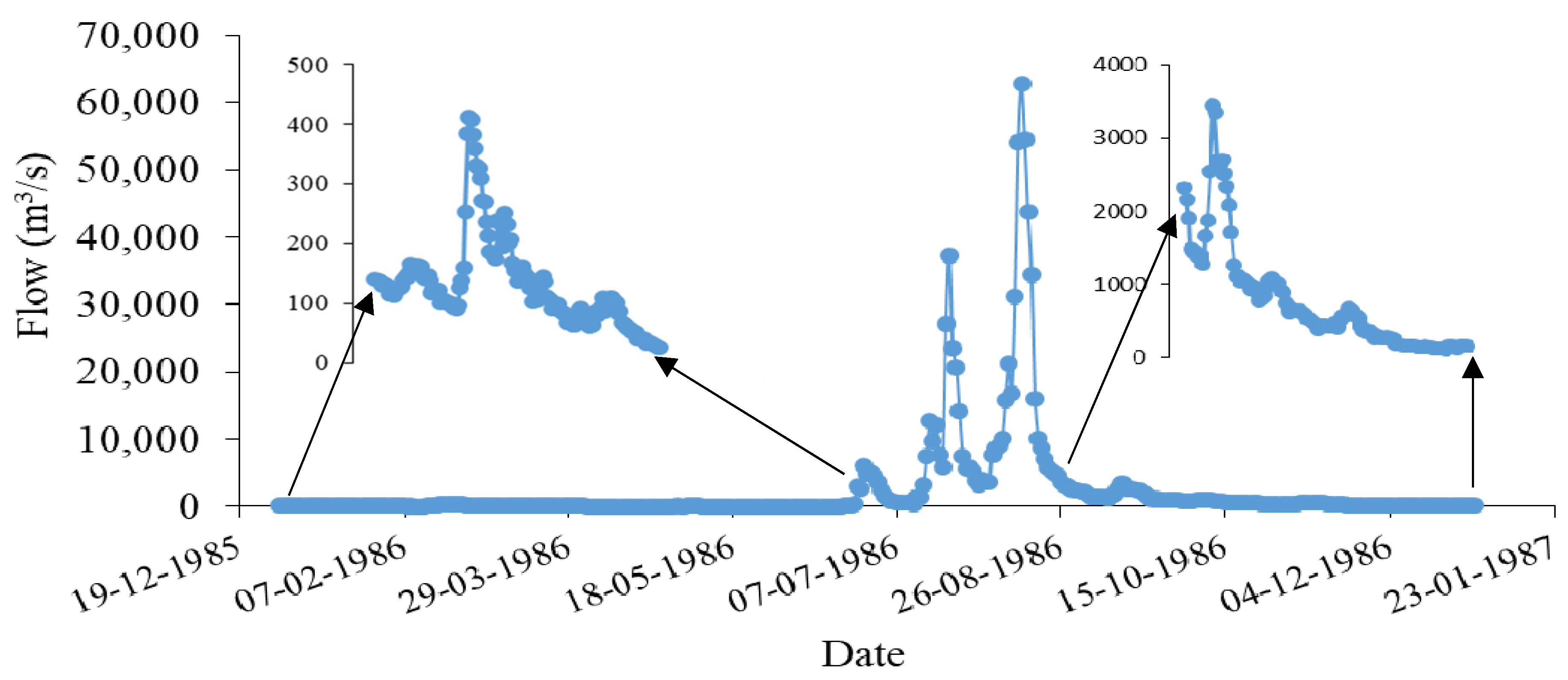
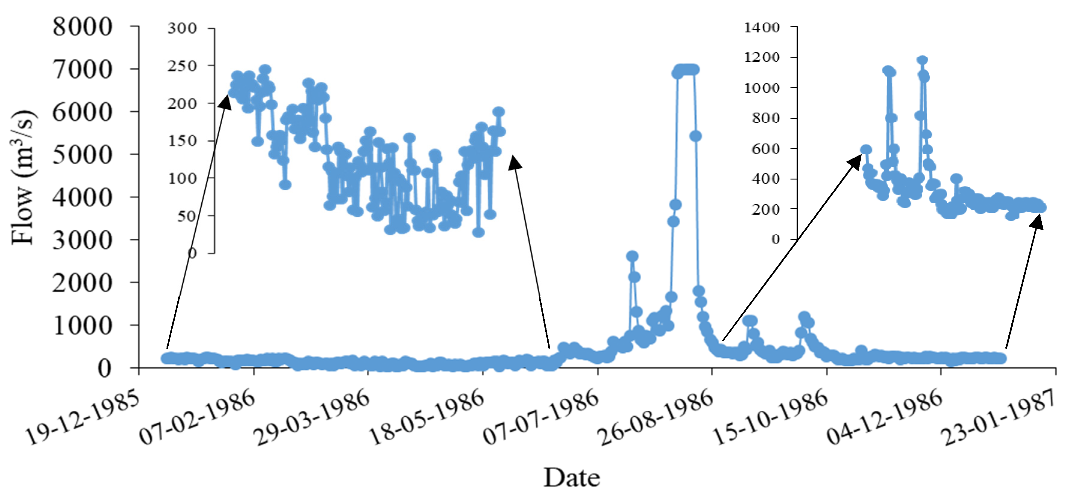
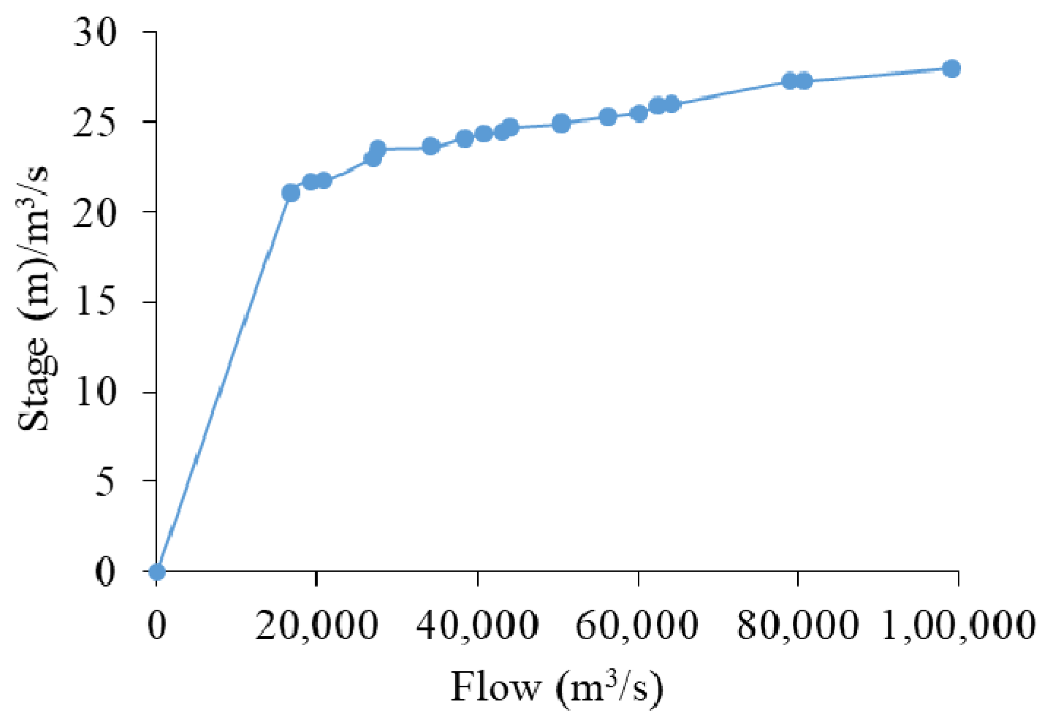
The flow data consists of boundary conditions (external and internal), as well as initial conditions. Boundary conditions are established at all open ends of the river system [32]. Upstream ends of a river system are modeled with the flow hydrograph (most common upstream boundary condition) boundary conditions. Downstream ends of the river system are modeled with the rating curve. The boundary conditions used in this study, depending on the availability of data for unsteady flow calculations, were given in Table 3. Flow hydrograph is considered as Upstream boundary condition at Dummugudem and Konta for observed discharges in the year 1986, as shown in Figure 5 and Figure 6. A rating curve is taken as a boundary condition for downstream location Polavaram, as shown in Figure 7. For the present study, the momentum equation (Equations (4) and (5)) is applied on Sabari–Sileru rivers confluence at Kunta and Sabari - Godavari rivers confluence at Kunavaram. A blow-up of water surface profile obtained using momentum equation corresponding to discharge predicted at 1000 and 10,000 years at Kunavaram junction.
Continuity equation
Conservative form
where Q is the total flow (m3/s), A is total flow area (m2), a function of distance, x, and time t, and qt is the lateral inflow per unit length (m2/s).
Momentum equation
Conservative form
where Q id the total flow (m3/s) as a function of distance, x, and time, t, V is the control volume (m3), g is the gravity acceleration (m/s2), A is the total area (m2), is the water surface slope (dimensionless), and is the friction slope (dimensionless).
3.4.3. A Combined 1D–2D Unsteady Flow Model
The 2D unsteady flow equation solver was developed at HEC and was directly integrated into the HEC-RAS Unsteady flow engine to facilitate combined 1D and 2D hydrodynamic modeling. HEC-RAS’s 1D and 2D unsteady-flow routing has proved the ability to perform on a more large river system, whereas 2D modeling is always considered in the areas that require a higher level of hydrodynamic precision [33]. The coupled 1D and 2D algorithms allow for direct feedback for each time step between flow elements, which results in accurate calculation of all types of flow and submergence at the hydraulic structure on a time-step-by-step basis, as used by Brunner [27].
Diffusion wave equations (Equation (5)) are most applicable in subcritical flows where the effects of viscosity prevail, and the consequences of inertia are not pronounced. Full dynamic wave equations (shallow-water equations) are applicable in almost all hydraulic problems [15].
In the HEC-RAS 1D–2D combined method, a lateral connection is used, in which the 2D flow areas are coupled to the 1D cross-sections using a lateral structure (Polavaram dam in this study). The hydraulic calculations that were developed for the steady flow component were incorporated into the unsteady flow module. The new 2D solver uses a finite volume solution algorithm, which can handle subcritical, supercritical, and mixed flow regime (including hydraulic jumps), much more robustly than the current 1D finite difference solution scheme [14,27].
The new 2D Flow Area option in HEC-RAS allows users to model areas with either the shallow-water equations in two-dimensions or the Diffusion Waveform of the equations in two-dimensions as shown below [1,34].
Shallow-water equations (full momentum):
The 2D diffusion wave equations, used in this study, allow the software to run faster and have greater stability properties [27]. Floodplain flow is thus approximated as a two-dimensional diffusion wave:
Diffusion Wave Equation:
where, C = Courant Number (dimensionless), V is the velocity of the flood wave (m/s), is the computational time step (s), and is the average cell size (m).
3.4.4. Manning’s N
The selection of an appropriate value for Manning’s n is quite significant for the accuracy of the computed water surface profiles. The value of Manning’s n is highly variable and depends on several factors, including the type of riverbed, flood plain characteristics, type of vegetation, channel irregularities, channel alignment, obstructions, size and shape of the channel, suspended material, and bedload. Manning’s n values were not calibrated as observed water surface elevation information at various locations of the study area (gaged data, as well as high water marks) or experimental data was not available. For water surface profile computations, a composite Manning’s roughness coefficient of 0.035 was considered as suggested in Chow’s book “Open-Channel Hydraulics” [1] and HEC-RAS reference manual [27] based on type and size of materials that compose the bed and banks of a channel, and the shape of the channel.
3.4.5. Creating the 2D Computational Mesh
The HEC-RAS terminology for describing the computational mesh for 2D modeling begins with the 2D flow area. For 2D computations, HEC-RAS uses a hybrid discretization scheme combining finite difference and finite volume methods [29].
It is found in various studies that the sole use of topographic data is too dense to be realistically used as a grid for numerical a [14]. Recent advances in HEC-RAS 2D modeling include the adaptive mesh refinement method [35]. HEC-RAS uses the sub-grid bathymetry approach, where the extra water levels are pre-computed from fine bathymetry. The high-resolution details are neglected, but enough data are available so that the coarser numerical method can account for the fine bathymetry through mass conservation [29]. The 2D flow area defines the boundary for which 2D computations will occur. The computational mesh is created within the 2D flow area. In the present study, the mesh shown in Figure 1 and Figure 4 contains 46,584 cells. Computational points spacing has been taken as = 200 m and = 200 m.
4. Results and Discussion
4.1. Statistical Analysis of the Data
The descriptive statistical analysis for the data obtained from the Dowleswaram and Polavaram source is given in Table 4. The mean, variance, standard deviation, skewness coefficient, coefficient of variation, and excess kurtosis were presented. Where the mean flood discharge is 44,445 m3/s for Dowleswaram and 30,277 m3/s for Polavaram data. The distribution of flood discharge was found to be positively skewed for both data sets. The chi-square test was calculated for eight probability distributions for both Dowleswaram and Polavaram data. The probability distributions for flood discharge were ranked based on the goodness of the fit and presented in Table 5. It was observed that Normal and Weibull performed well in the chi-square test. Based on the values of statics, normal distribution was used for the estimation of flood peaks for both Polavaram and Dowleswaram discharge data.
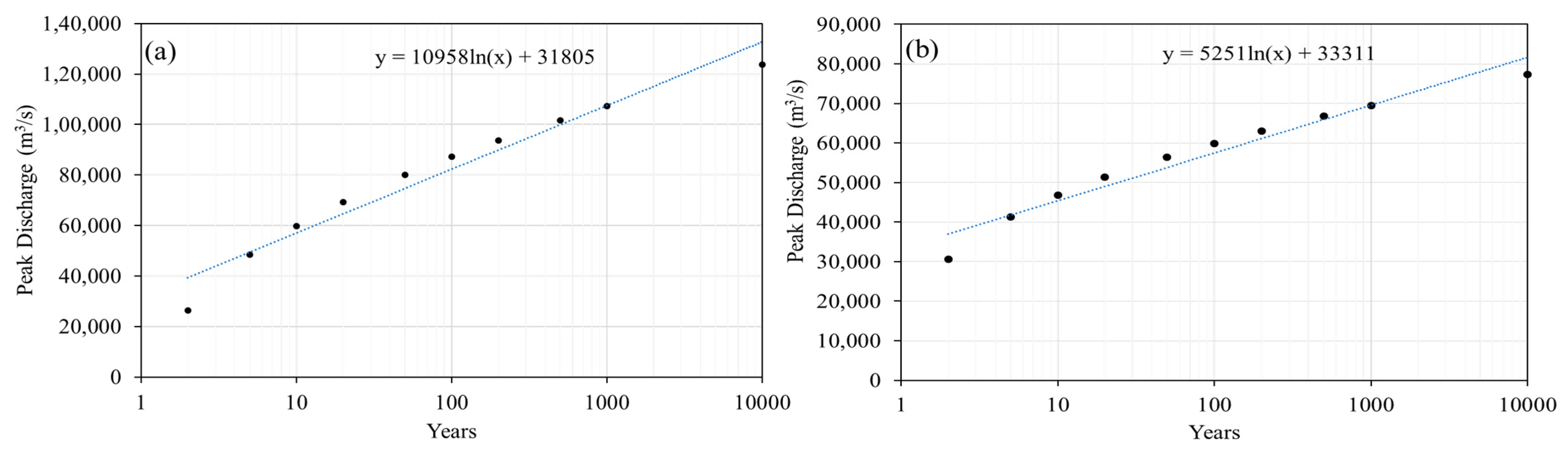
The discharge flow derived from the normal distribution for the return periods of 2, 5, 10, 20, 50, 100, 200, 500, 1000, and 10,000 years were shown in Figure 8, which is used as steady flow inputs in HEC-RAS at 5 sections. The boundary condition applied at the end of each reach was given in Table 2. The first section was at river Godavari reach from Dummugundem to Kunnavaram, the second section at river Saberi reach from Kunta to Saberi, the third section at river sileru reach from Kunta to sileru, the fourth section at Saberi reaches from Kunnavaram to Kunta, the fifth section at Godavari river reaches from Kunnavaram to Polavaram. The discharge distribution obtained for different reach is given in Table 6. It shows the input values given for both Dowleswaram and Polavaram location data sets for 1000 and 10,000 years return period.
4.2. Water Surface Elevations (WSE)
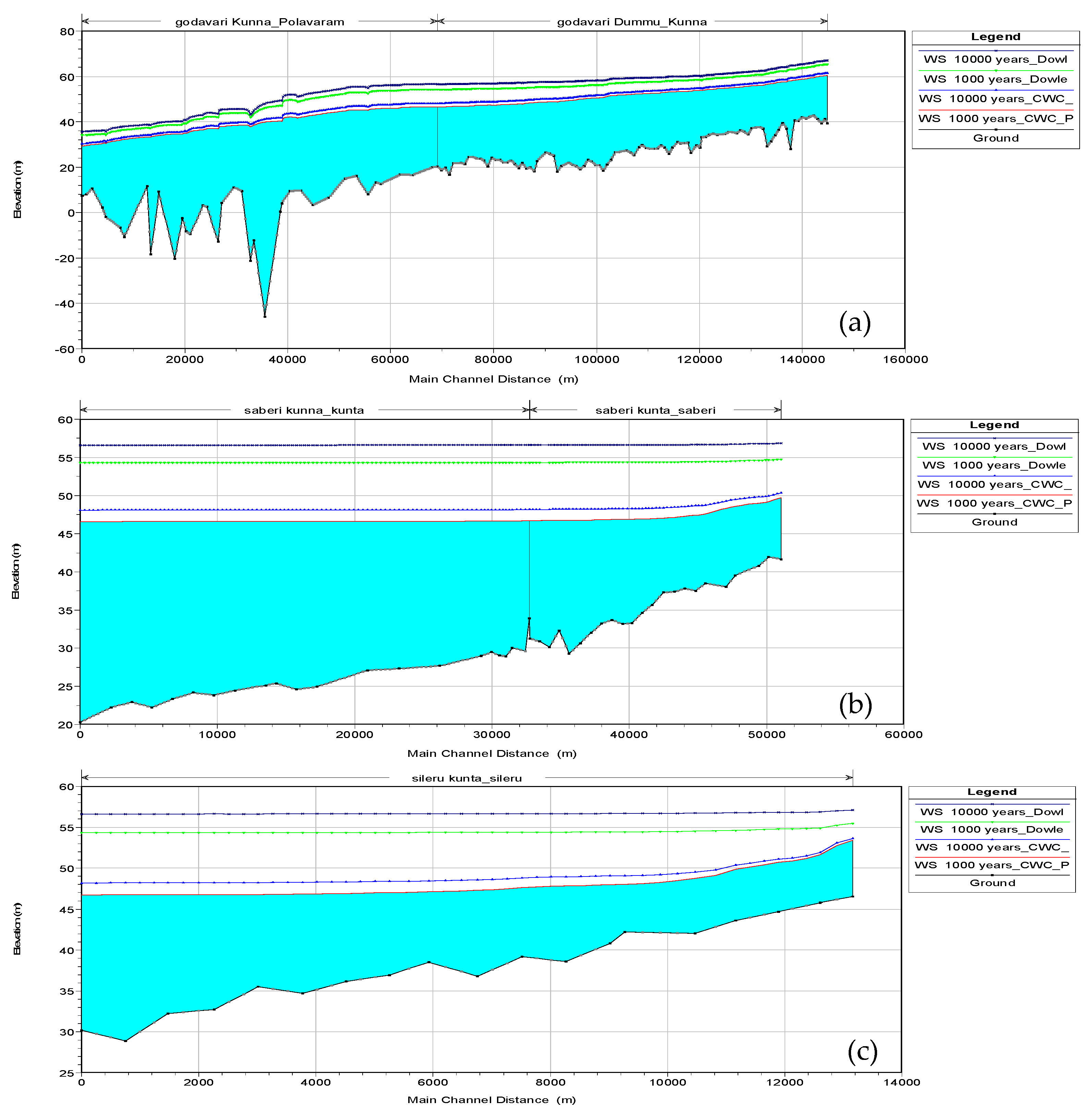
A comparative illustration of WSE for 1000 and 10,000 years discharge considering Polavaram and Dowleswaram data at different reach sections Polavaram to Dummugudem, Kunavaram to Saberi along river Saberi and Kunta to Sileru is shown in Figure 9. The WSE produced by Dowleswaram data is higher than that produced by the Polavaram data set for both 1000 and 10,000-year return-period, thus indicating the differences in data and severity of floods. Water surface profile data were extracted from HEC-RAS through HEC-GeoRAS and then incorporated into a floodplain. The water surface profiles at Bhadrachalam with and without dam under 1D steady-state conditions are given in Table 7. It shows water levels for discharges 0.10 and 0.14 million m3/s and 1000 years flood (full closure and 50% opening of gates) and 10,000 years flood.
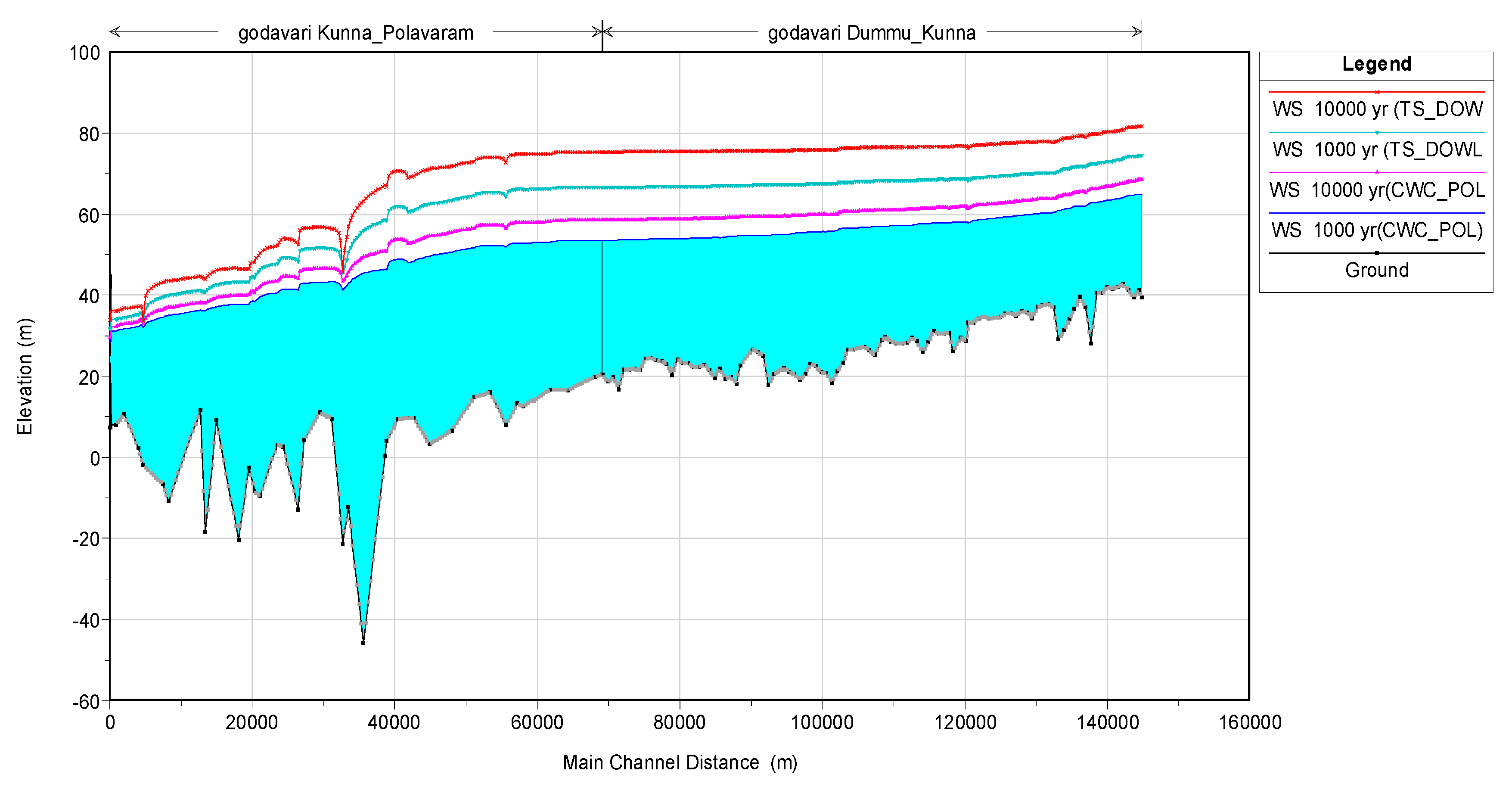
The most of built-up areas in Bhadrachalam will be submerged for the computed discharges, along with which all the neighboring villages underwater. As the discrepancy between Dowleshwaram and CWC data (Polavaram location) can be seen evidently, we simulated the water surface elevation for 1000 and 10,000 years discharge considering discharge data at Dowleswaram and corresponding water levels at Polavaram as shown in Figure 10. Water surface levels at Bhadrachalam with and without dam for different discharges under 2D unsteady state conditions are shown in Table 8. As gate operations are done for 1D steady-state showed a difference in upstream levels, for 2D unsteady state conditions we operated gates at 50% and 100% (10 m and 20 m heights of the gate). The WSE with dam for 1000 and 10,000 years of 59.11 m and 60.89 m was obtained and without dam 58.29 m and 59.98 m at Bhadrachalam respectively. By considering Dowleswaram discharge data and Polavaram water levels at Polavaram WSE at Bhadrachalam were found as 57.78 m and 61.43 m (with a dam) 57.77 m and 61.41 m (Without dam) for 1000 and 10,000 years respectively at Bhadrachalam. The results showed that with half of the gates as open and, all gates closed water surface elevation of 62.34 m and 72.34 m were obtained at Bhadrachalam for 1000 and 10,000 years respectively.
4.3. Discussions
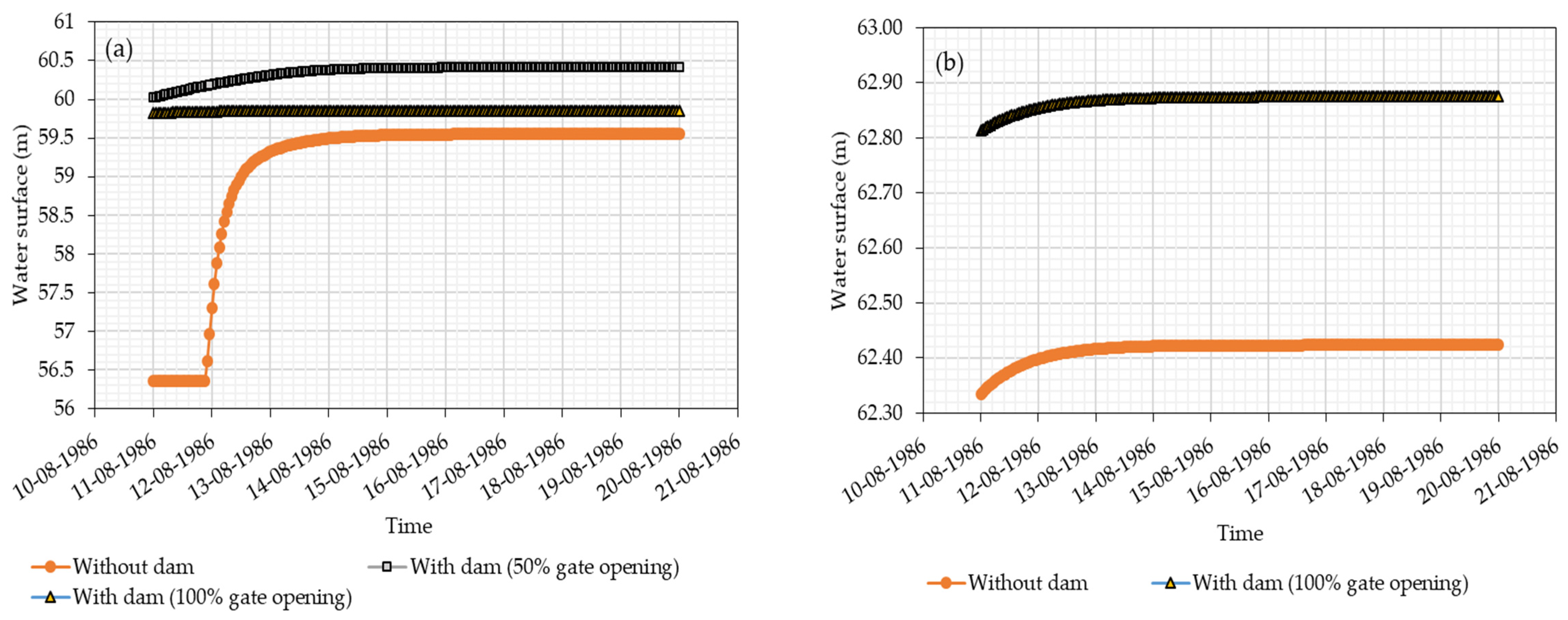
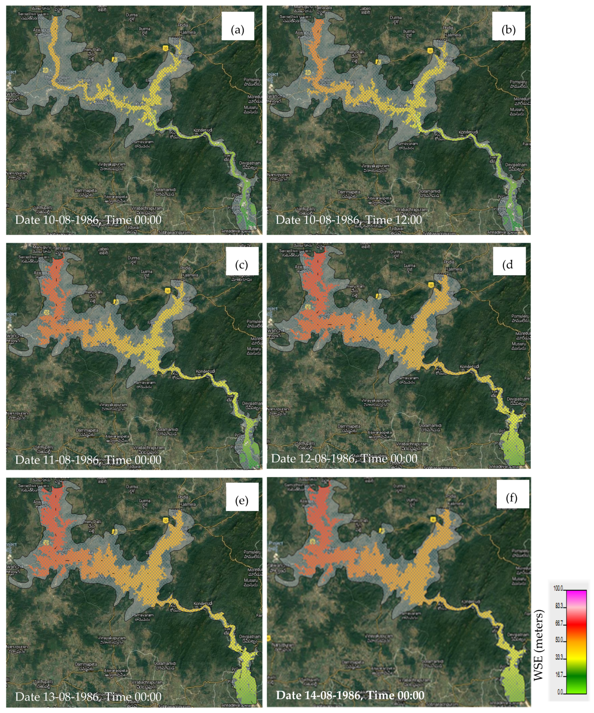
The submergence (flood) maps were produced using elevation (DEM), River geometry, cross-section data, and flood discharge values. The 2D unsteady flow simulated for (a) 0.10 million m3/s and (b) 0.14 million m3/s with and without a dam from the period 11 to 20 August 1986 is shown in Figure 11. This indicates the effect of the dam on the upstream areas, even with a minimum of 0.10 million m3/s discharge will be catastrophic at Bhadrachalum. As we have already experienced 0.09 million m3/s discharge flood in the past [18]. The Polavaram project has been designed for 0.10 million m3/s, based on which consequences in the upstream submergence during a flood event is under looked. In Figure 12, the inundation map simulated for 0.10 million m3/s discharge from 11 to 20 August 1986 period. The inundation figures (Figure 12) show that most of Bhadrachalam town will be under submergence for the computed discharges, along with all built-up, agricultural areas in the neighborhood.
The previous studies existing on backwater computation in the region were carried out for only 1-D simulations. Our study has presented both 1D-2D models to estimate backwater levels and values were found acceptable. The unsteady flow simulations show a lesser water level than steady-state at Bhadrachalam, the reason being an increase in the 2D spread area. From 2D unsteady flow simulations with and without dam and gate operations show that with improper operating of gates and even for minimum 0.10 million m3/s discharge, water levels at Bhadrachalam will be high enough to submerge prime locations and its vicinity. Our simulation results mimicking the maximum flood event that occurred in the region from 11 to 20 August 1986 clearly indicate submergence zones. It was found from this study that the existing Polavaram dam will cause a severe threat to the upstream region even with a minimum flood event. Therefore, the large dam projects should be dealt with intensive planning and public discussion by engineers and policymakers.
5. Conclusion and Recommendation
The discharge data obtained from two different departments were analyzed and found that Dowleswaram data is more appropriate and reliable for study. Along with these two data sets, we have also carried out the combined study by considering Dowleswaram discharges at Polavaram location with actual water levels observed at Polavaram and found significant changes in WSE. Among the best-fitted distribution, top-ranked distributions namely Normal distributions were considered and WSE were calculated.
The unsteady flow simulations show a lesser water level than steady at Bhadrachalam, the reason being an increase in the 2D spread area. From 2D unsteady flow simulations, with and without dam and gate operations show that with improper operating of gates and even for minimum 0.1 million m3/s discharge, water levels at Bhadrachalam will be high enough to submerge prime locations and its vicinity.
Moreover, it is essential to mention that the scope of the presented paper did not exhaust the presence of bridges and other hydraulic structures along with a dam. Indeed, besides the effect induced by a dam, the role played by erosion, sediment transport, and debris cannot be ignored. It has to be mentioned that no uncertainty analysis was carried out, which might affect the presented analysis. Backwater floods as a hydrological phenomenon do not manifest itself as a flood wave or as a highly intense wave. Hence, human life losses are rare, but economic damage caused can be significant. The following recommendations are made from our study to prevent the possible risk of submergence and resulting losses. Regular and periodic maintenance of the gates of the Polavaram dam is a must for the safety of upstream areas. Dam gates should be well operated, keeping in mind the inflows and submergence that would cause by improper closing/opening of the gate walls. Construction of levees and dredging of riverbed may be suggested in the regions to reduce the water surface elevation.
Author Contributions
A.C.R.: Conceptualization, Data curation, Formal analysis, Investigation, Methodology, Visualization, Writing-Original draft preparation. S.T.: Conceptualization, Formal analysis, Funding acquisition, Investigation, Methodology, Project administration, Supervision, Visualization, writing review and editing. All authors have read and agreed to the published version of the manuscript.
Funding
This research was funded by The Interstate and Water Resources wing of Irrigation and CAD Department, Government of Telangana.
Acknowledgments
We like to thank Central Water Commission (CWC), Hyderabad office, Telangana, for providing necessary data and reports. We would also like to acknowledge S Narasimha Rao, Engineer, ISWR (Inter State Water Resources) Wing of Irrigation and CAD Department, Government of Telangana, and his colleagues for constant support and clarification about data. We thank R. Srinivasan, Texas A&M for suggesting us to publish in this journal.
Conflicts of Interest
The authors declare no conflict of interest.
References
- Chow, V.T. Open-channel hydraulics. International student edition. In McGraw-Hill Civil Engineering Series; McGraw-Hill: Tokyo, Japan, 1959. [Google Scholar]
- Yang, Y.; Zhang, M.; Zhu, L.; Liu, W.; Han, J.; Yang, Y. Influence of Large Reservoir Operation on Water-Levels and Flows in Reaches below Dam: Case Study of the Three Gorges Reservoir. Sci. Rep. 2017, 7, 1–14. [Google Scholar] [CrossRef] [PubMed] [Green Version]
- Volke, M.A.; Johnson, W.C.; Dixon, M.D.; Scott, M.L. Emerging reservoir delta-backwaters: Biophysical dynamics and riparian biodiversity. Ecol. Monogr. 2019, 89, e01363. [Google Scholar] [CrossRef] [Green Version]
- Liro, M. Dam reservoir backwater as a field-scale laboratory of human-induced changes in river biogeomorphology: A review focused on gravel-bed rivers. Sci. Total Environ. 2019, 651, 2899–2912. [Google Scholar] [CrossRef] [PubMed]
- Maselli, V.; Pellegrini, C.; Del Bianco, F.; Mercorella, A.; Nones, M.; Crose, L.; Guerrero, M.; Nittrouer, J.A. River Morphodynamic Evolution Under Dam-Induced Backwater: An Example from the Po River (Italy). J. Sediment. Res. 2018, 88, 1190–1204. [Google Scholar] [CrossRef] [Green Version]
- Scott, S.H.; Sharp, J.A.; Savant, G. Two Dimensional Hydrodynamic Analysis of the Moose Creek Floodway; No. ERDC/CHL-TR-12-20; Engineer Research and Development Center Vicksburg MS Coastal and Hydraulics Lab, 2017; Available online: https://erdc-library.erdc.dren.mil/xmlui/bitstream/handle/11681/21022/ERDC-ITL%20SR-17-1.pdf?sequence=1&isAllowed=y (accessed on 11 December 2019).
- Sheng, B. Hydraulic Structure and Stream Vegetation Induced Backwater Effects on Wetland Flood Reduction. Ph.D. Thesis, University of Wisconsin-Madison, Madison, WI, USA, 2014. [Google Scholar]
- Teo, F.Y. Study of the Hydrodynamic Processes of Rivers and Floodplains with Obstructions. Ph.D. Thesis, Cardiff University, Cardiff, UK, 2010; p. 254. [Google Scholar]
- Costabile, P.; Macchione, F.; Natale, L.; Petaccia, G. Comparison of scenarios with and without bridges and analysis of backwater effect in 1-D and 2-D river flood modeling. Comput. Model. Eng. Sci. 2015, 109, 81–103. [Google Scholar]
- Macchione, F.; Viggiani, G. Simple modelling of dam failure in a natural river. Proc. Inst. Civ. Eng. Water Manag. 2004, 157, 53–60. [Google Scholar] [CrossRef]
- Khattak, M.S.; Anwar, F.; Saeed, T.U.; Sharif, M.; Sheraz, K.; Ahmed, A. Floodplain Mapping Using HEC-RAS and ArcGIS: A Case Study of Kabul River. Arab. J. Sci. Eng. 2016, 41, 1375–1390. [Google Scholar] [CrossRef]
- Teng, J.; Jakeman, A.J.; Vaze, J.; Croke, B.F.W.; Dutta, D.; Kim, S. Flood inundation modelling: A review of methods, recent advances and uncertainty analysis. Environ. Model. Softw. 2017, 90, 201–216. [Google Scholar] [CrossRef]
- Patel, D.P.; Ramirez, J.A.; Srivastava, P.K.; Bray, M.; Han, D. Assessment of flood inundation mapping of Surat city by coupled 1D/2D hydrodynamic modeling: A case application of the new HEC-RAS 5. Nat. Hazards 2017, 89, 93–130. [Google Scholar] [CrossRef]
- Lea, D.; Yeonsu, K.; Hyunuk, A. Case study of HEC-RAS 1D-2D coupling simulation: 2002 Baeksan flood event in Korea. Water 2019, 11, 2048. [Google Scholar] [CrossRef] [Green Version]
- Guidelines for Assessing and Managing Risks Associated with Dams. Available online: https://www.damsafety.in/ecm-includes/PDFs/Guidelines_on_Risk_Analysis.pdf (accessed on 15 October 2019).
- Welcome to Godavari Basin. Available online: http://www.sakti.in/godavaribasin/indira-ICad.htm (accessed on 1 November 2019).
- Flood Category Wise Abstract. Available online: http://india-water.gov.in/ffs/flood-forecasted-bulletins/ (accessed on 9 October 2019).
- Flood Forecasting/Hydrological Observation|Central Water Commission. Available online: http://www.cwc.gov.in/flood-forecasting-hydrological (accessed on 9 October 2019).
- Comptroller and Auditor General of India. Report of the Comptroller and Auditor General of India On National Projects Union Government Ministry of Water Resources, River Development and Ganga Rejuvenation Report No. 6 of 2018 (Performance Audit); 2018. Available online: https://cag.gov.in/content/report-no6-2018-performance-audit-national-projects-ministry-water-resources-river (accessed on 11 November 2019).
- Polavaram Dam—A Critical View on Ecological Governance|Environics Trust. Available online: http://environicsindia.in/2011/05/17/polavaram-dam-a-critical-view-on-ecological-governance/ (accessed on 9 October 2019).
- Rao, P.T. Nature of Opposition to the Polavaram Project. Econ. Political Wkly. 2006, 41, 1437–1439. [Google Scholar]
- Mariotti, C. Displacement, Resettlement and Adverse Incorporation in Andhra Pradesh. The Case of the Polavaram Dam. Ph.D. Thesis, SOAS, University of London, London, UK, 2012. [Google Scholar]
- Stewart, T.; Rukmini Rao, V. India’s Dam shame: Why Polavaram Dam Must not be Built Andhra Pradesh; Gramya Resource Centre for Women: Hyderabad, India, 2006; Available online: https://conflicts.indiawaterportal.org/sites/conflicts.indiawaterportal.org/files/India’sDamShame-WhyPolavaramDammustnotbebuilt-2006.pdf (accessed on 1 September 2018).
- Feldes, K. Imaginaries of development: A case study of the Polavaram Dam Project. Interdiszip. Zeitschrift für Südasienforsch. 2017, 1, 71–112. [Google Scholar]
- Godavari Water Disputes Tribunal; 1980; Volume I. Available online: http://cwc.gov.in/sites/default/files/GWDTAward%20Further%20Report.pdf (accessed on 11 December 2019).
- No Guidelines on Studying Backwater Impact of Dams: CWC-RTI in Media-RTI INDIA-Online RTI. Available online: https://rtiindia.org/forums/topic/64252-no-guidelines-on-studying-backwater-impact-of-dams-cwc/ (accessed on 11 December 2019).
- HEC-RAS. River Analysis System Hydraulic Reference Manual. 2016. Available online: https://www.hec.usace.army.mil/software/hec-ras/documentation/HEC-RAS%205.0%20Reference%20Manual.pdf (accessed on 11 December 2019).
- Ackerman, P.E.C.T. HEC-GeoRAS: GIS Tools for Support of HEC-RAS using ArcGIS®. In US Army Corps Engineers Hydrologic Engineering Center. User’s Manual. Version 4.2; 2009; p. 244. Available online: https://www.hec.usace.army.mil/software/hec-georas/documentation/HEC-GeoRAS42_UsersManual.pdf (accessed on 11 December 2019).
- Brunner, G.W.; Warner, J.C.; Wolfe, B.C.; Piper, S.S. Guía de Aplicaciones HEC-RAS [HEC-RAS Applications Guide]. 2016. Available online: https://www.hec.usace.army.mil/software/hec-ras/documentation/HEC-RAS%205.0%20Applications%20Guide.pdf (accessed on 11 December 2019).
- US-ACE. HEC-RAS 5.0.3 Release Notes; 2016. Available online: https://www.hec.usace.army.mil/software/hec-ras/documentation/HEC-RAS_5.0.5_Release%20Notes.pdf (accessed on 11 December 2019).
- Barkau, R.L. UNET, One-Dimensional Unsteady Flow through A fulL Network of Open Channels; Computer Program: St. Louis, MO, USA, 1992. [Google Scholar]
- Chanson, H. Unsteady open channel flows: 1. Basic equations. Environ. Hydraul. Open Channel Flows 2004, 185–222. [Google Scholar] [CrossRef]
- Betsholtz, A.; Nordlöf, B. Potentials and Limitations of 1D, 2D and Coupled 1D-2D Flood Modelling in HEC-RAS: A Case Study on Höje River; Lund University: Lund, Sweden, 2017; p. 128. [Google Scholar]
- Chanson, H. Fundamentals of open channel flows. In Environ. Hydraul. Open Channel Flows; 2004; pp. 11–34. [Google Scholar] [CrossRef] [Green Version]
- An, H.; Yu, S.; Lee, G.; Kim, Y. Analysis of an open source quadtree grid shallow water flow solver for flood simulation. Quat. Int. 2015, 384, 118–128. [Google Scholar] [CrossRef]
Figure 1.
Study area location in Godavari basin from Dummugudem and konta in upstream of Godavari River till Polavaram project location with 2D flow area considered with cross-sections.
Figure 1.
Study area location in Godavari basin from Dummugudem and konta in upstream of Godavari River till Polavaram project location with 2D flow area considered with cross-sections.

Figure 2.
Flow chart of the methodology.

Figure 3.
Observed peak annual discharge at Polavaram and Dowleswaram gauge.

Figure 4.
DEM (30 m × 30 m) map and cross-section data considered for the study.

Figure 5.
Flow hydrograph data considered for upstream boundary condition at Dummugudem for the year 1986.
Figure 5.
Flow hydrograph data considered for upstream boundary condition at Dummugudem for the year 1986.

Figure 6.
Flow hydrograph data considered for upstream boundary condition at Konta for the year 1986.
Figure 6.
Flow hydrograph data considered for upstream boundary condition at Konta for the year 1986.

Figure 7.
Rating curve data considered for downstream boundary condition at Polavaram for the year 1986.
Figure 7.
Rating curve data considered for downstream boundary condition at Polavaram for the year 1986.

Figure 8.
Discharges at (a) Dowleswaram and (b) Polavaram obtained using normal distributions.

Figure 9.
Water surface elevation for 1000 and 10,000 years discharge considering Polavaram and Dowleswaram data from (a) Polavaram to Dummugudem (b) Kunnavaraam to Saberi along river Saberi and (c) Konta to Sileru.
Figure 9.
Water surface elevation for 1000 and 10,000 years discharge considering Polavaram and Dowleswaram data from (a) Polavaram to Dummugudem (b) Kunnavaraam to Saberi along river Saberi and (c) Konta to Sileru.

Figure 10.
Water surface elevation for 1000 and 10,000 years discharge (considering discharge data at Dowleswaram and corresponding water levels at Polavaram) from Polavaram to Dummugudem.
Figure 10.
Water surface elevation for 1000 and 10,000 years discharge (considering discharge data at Dowleswaram and corresponding water levels at Polavaram) from Polavaram to Dummugudem.

Figure 11.
2D unsteady flow simulated for (a) 0.10 million m3/s with and without dam (b) 0.14 million m3/s discharge with and without a dam.
Figure 11.
2D unsteady flow simulated for (a) 0.10 million m3/s with and without dam (b) 0.14 million m3/s discharge with and without a dam.

Figure 12.
Simulated inundation map for a period of 10th –14th August 1986 without a dam. (a) and (b) shows inundation on 10th August 1986 at gap of 12 h. (c), (d), (e) and (f) shows inundation from 11th to 14th August at 00:00 hours.
Figure 12.
Simulated inundation map for a period of 10th –14th August 1986 without a dam. (a) and (b) shows inundation on 10th August 1986 at gap of 12 h. (c), (d), (e) and (f) shows inundation from 11th to 14th August at 00:00 hours.


Table 1.
List of Data collected from different sources.
| Source | Discharge Data | Cross-sections Data Across the Godavari | Spillway Details | Others |
|---|---|---|---|---|
| Central Water Commission (CWC) | For whole Godavari basin | Seven different locations from Polavarma to Dummugudem | NA | Zero of gauges, Hourly water levels |
| Inter-State and Water Resources, Hyderabad | NA | Polavaram to Dummugudem | spillway design | Reports on the Godavari |
| Telangana State department | Annual discharge data at Dowleshwaram | NA | NA | NA |
NA—Not available.
Table 2.
Boundary conditions applied at the end of each reach for the 1D steady flow.
| River | Reach | Upstream | Downstream |
|---|---|---|---|
| Godavari | Dummugudem to Kunnavaram | Rating Curve | Junction 1 |
| Saberi | Kunta to Saberi | Rating Curve | Junction 2 |
| Siler | Kunta to Sileru | Rating Curve | Junction 2 |
| Saberi | Kunnavaram to Kunta | Junction 2 | Junction 1 |
| Godavari | Kunnavaram to Polavaram | Junction 1 | Rating Curve |
Table 3.
Boundary conditions considered for 2D unsteady flow.
| River | Location | Boundary Condition |
|---|---|---|
| Godavari | At Dummugudem | Flow Hydrograph |
| Godavari | At Polavaram | Rating Curve |
| Saberi | At Kunta | Flow Hydrograph |
Table 4.
Descriptive statistics for flood discharge in Dowleswaram and Polavaram (S.I units).
| Statistic | Dowleswaram Data | Polavaram Data |
|---|---|---|
| Mean | 44,445 | 30,277 |
| Standard Error | 3892 | 1764 |
| Median | 42,439 | 29,786 |
| Mode | 34,274 | 19,062 |
| Standard Deviation | 22,018 | 12,596 |
| Sample Variance | 4.85 × 10⁸ | 1.59 × 10⁸ |
| Kurtosis | −0.02177 | −0.013388 |
| Skewness | 0.59469 | 0.15411 |
| Range | 88,180 | 61,368 |
| Minimum | 11,082 | 289 |
| Maximum | 99,262 | 61,658 |
| Sum | 1,422,255 | 1,544,104 |
| Sample size | 32 | 51 |
Table 5.
Goodness of fit test (Chi-square test) for probability distributions along with rank.
| At Dowleswaram | At Polavaram | |
|---|---|---|
| Distribution | Rank | Rank |
| Gamma | 8 | 4 |
| Gen. Extreme Value | 3 | 2 |
| Lognormal (3P) | 5 | 1 |
| Log-Pearson 3 | 7 | 7 |
| Normal | 1 | 3 |
| Pearson 5 (3P) | 4 | 6 |
| Pearson 6 (4P) | 6 | 5 |
| Weibull | 2 | 8 |
Table 6.
Discharge distribution in m3/s considered for steady-state analysis at different reaches.
| River | Reach | Dowleswaram | Polavaram Data | ||
|---|---|---|---|---|---|
| 1000 Year | 10,000 Years | 1000 Year | 10,000 Years | ||
| Godavari | Dummuguddem to Kunnavaram | 104,988 | 117,910 | 64,820 | 72,186 |
| Saberi | Kunta to saberi | 4999 | 5615 | 3087 | 3437 |
| Sileru | Kunta to Sileru | 2500 | 2807 | 1543 | 1719 |
| Saberi | Kunnavaram to Kunta | 7499 | 8422 | 4630 | 5156 |
| Godavari | Kunnavaram to Polavaram | 112,487 | 126,332 | 69,450 | 77,342 |
Table 7.
Water surface levels at Bhadrachalam with and without dam for different discharges under 1D steady-state conditions.
Table 7.
Water surface levels at Bhadrachalam with and without dam for different discharges under 1D steady-state conditions.
| Discharge (m3/s) | With Dam (m) | Without Dam (m) |
|---|---|---|
| 0.10 million | 57.02 | 57.00 |
| 0.14 million | 61.79 | 61.77 |
| 1000 Years flood (0.11 million) | 57.78 | 57.77 |
| 10,000 Years flood (0.13 million) | 61.43 | 61.41 |
| 1000 Years flood (0.11 million, by considering 50% opening of gates) | 62.34 | NA * |
Table 8.
Water surface levels at Bhadrachalam with and without dam for different discharges under 2D unsteady state conditions.
Table 8.
Water surface levels at Bhadrachalam with and without dam for different discharges under 2D unsteady state conditions.
| Discharge (m3/s) | With Dam (m) | Without Dam (m) | |
|---|---|---|---|
| For 50% Gate Opening Height | For 100% Gate Closure Height | ||
| 0.10 million | 60.03 | 59.84 | 59.52 |
| 0.14 million | 63.13 | 62.85 | 62.38 |
| For Observed CWC discharge data (0.14 million) | 63.20 | 62.81 | 62.50 |
© 2020 by the authors. Licensee MDPI, Basel, Switzerland. This article is an open access article distributed under the terms and conditions of the Creative Commons Attribution (CC BY) license (http://creativecommons.org/licenses/by/4.0/).
Share and Cite
MDPI and ACS Style
C R, A.; Thatikonda, S. Study on Backwater Effect Due to Polavaram Dam Project under Different Return Periods. Water 2020, 12, 576. https://doi.org/10.3390/w12020576
AMA Style
C R A, Thatikonda S. Study on Backwater Effect Due to Polavaram Dam Project under Different Return Periods. Water. 2020; 12(2):576. https://doi.org/10.3390/w12020576
Chicago/Turabian StyleC R, Amarnath, and Shashidhar Thatikonda. 2020. "Study on Backwater Effect Due to Polavaram Dam Project under Different Return Periods" Water 12, no. 2: 576. https://doi.org/10.3390/w12020576
Note that from the first issue of 2016, this journal uses article numbers instead of page numbers. See further details here.