Improving the Accuracy of Hydrodynamic Model Predictions Using Lagrangian Calibration
by
 , and
, and
Neda Mardani
1,*, 
Kabir Suara
2,
Helen Fairweather
1,
Richard Brown
2,
Adrian McCallum
1 and
Roy C. Sidle
3,4 1
Civil and Environmental Engineering, University of the Sunshine Coast, Sippy Downs, QLD 4556, Australia
2
Environmental Fluid Mechanics Group, Queensland University of Technology, Brisbane, QLD 4000, Australia
3
Sustainability Research Centre, University of the Sunshine Coast, Sippy Downs, QLD 4556, Australia
4
Mountain Societies Research Institute, University of Central Asia, Khorog 736112, Tajikistan
*
Author to whom correspondence should be addressed.
Water 2020, 12(2), 575; https://doi.org/10.3390/w12020575
Submission received: 31 December 2019
/
Revised: 12 February 2020
/
Accepted: 17 February 2020
/
Published: 20 February 2020
(This article belongs to the Special Issue Study of Lagoons and Other Shallow Water Bodies Through the Application of Numerical Models)
Abstract
:While significant studies have been conducted in Intermittently Closed and Open Lakes and Lagoons (ICOLLs), very few have employed Lagrangian drifters. With recent attention on the use of GPS-tracked Lagrangian drifters to study the hydrodynamics of estuaries, there is a need to assess the potential for calibrating models using Lagrangian drifter data. Here, we calibrated and validated a hydrodynamic model in Currimundi Lake, Australia using both Eulerian and Lagrangian velocity field measurements in an open entrance condition. The results showed that there was a higher level of correlation (R2 = 0.94) between model output and observed velocity data for the Eulerian calibration compared to that of Lagrangian calibration (R2 = 0.56). This lack of correlation between model and Lagrangian data is a result of apparent difficulties in the use of Lagrangian data in Eulerian (fixed-mesh) hydrodynamic models. Furthermore, Eulerian and Lagrangian devices systematically observe different spatio-temporal scales in the flow with larger variability in the Lagrangian data. Despite these, the results show that Lagrangian calibration resulted in optimum Manning coefficients (n = 0.023) equivalent to those observed through Eulerian calibration. Therefore, Lagrangian data has the potential to be used in hydrodynamic model calibration in such aquatic systems.
1. Introduction
Hydrodynamic models are essential tools for estuarine and coastal management [1] and have been used in studies of water quality [2], sediment transport [3], and predicting the impact of different climatic scenarios on estuaries and coastal waters [4]. These models also play significant roles in flood forecasting, contaminant modelling, and changes to estuaries and coastal morphology [5,6,7]. However, many of these applications contain inaccuracies resulting from model uncertainties, including from physical and numerical aspects of shallow water flow. Topography, boundary conditions, time steps and modelling discretization and computational errors are the main sources of error that result in uncertainties in the models [8,9,10]. The governing equations may not account for such complex physical processes and their interactions. Simplifying the dimensions and forcing terms to conserve computations [11], and inaccuracies in the input data, such as boundary conditions and bathymetry, can also contribute uncertainties.
Model calibration and validation by refining model parameters are standard approaches for reducing uncertainties. Improving the accuracy of hydrodynamic model output through calibration and validation is achieved by tuning the model parameters using a systematic comparison of simulated to measured data [12,13]. The accuracy of hydrodynamic model outputs is restricted by the quality and spatiotemporal coverage of available data. Direct measurement of water levels and velocities can contribute to the understanding of the hydrodynamics of tidal estuaries and provide a reliable source of data for the calibration and validation of hydrodynamic models [14]. To obtain confidence in this understanding, measurements must cover a range of spatial and temporal variabilities of velocities and water levels [15].
Flow parameters in estuaries have traditionally been obtained from Eulerian, fixed position devices such as Acoustic Doppler Velocimeters (ADV) and Acoustic Doppler Current Profilers (ADCP) [16]. An alternative is the Lagrangian approach in which drifters that move with the flow are deployed to obtain flow measurements [17,18]. While the Eulerian approach provides limited coverage and sparse measurements, a combined Eulerian–Lagrangian approach provides more insight into environmental hydrodynamics. ADCP can be supplemented by a cluster of GPS-tracked drifters to collect flow–current measurements in the domain of interest [19,20]. GPS-tracked drifters have proved to be an efficient instrument in characterizing the hydrodynamics of a water body as they provide both spatial and temporal coverage [21].
Drifters validated in surf zones [15,22] and more recently in tidal inlets and estuaries [17], showed that drifter-Lagrangian and fixed-device velocities agree well (R2 > 0.92) in a tidal inlet with depths ≤ 10 m and peak velocities ≤ 1 m/s. Suara et al. [23] extended the evaluation of drifter data into the inner section of a bounded tidal estuary with depth (2–3 m) and velocity (<0.5 m/s) using correlation, spectral, and coherence analyses. It was shown that drifters can assess surface flow dynamics of tidal waters in relation to large- and small-scale processes where ADCPs are not suitable. Although drifters can cover large areas, facilitating better insights into estuarine dynamics, a more complete study of such dynamics can only be achieved from hydrodynamics models. While recent efforts have focused on the use of Lagrangian drifters to examine flow dynamics of estuaries [24,25,26], there is limited work in evaluating the potential improvement in the accuracy of hydrodynamic models using Lagrangian drifter datasets.
Intermittently Closed and Open Lakes and Lagoons (ICOLLs) are a dynamic form of estuary which alternate between being open or closed to the ocean. They are mostly located in the South-East and South-West of the Australian mainland, as well as in Tasmania [27]. Major pressures on ICOLLs include sediment and nutrient transport and changes in entrance dynamics [28]. Recent studies highlight that nutrient inputs lowered the water quality in Eastern Australian ICOLLs [29]. Management issues are exacerbated by the cyclic nature of the entrance. Consequently, comprehensive spatio-temporal monitoring and modelling are necessary to fully investigate the dynamics of an ICOLL and enhance coastal management.
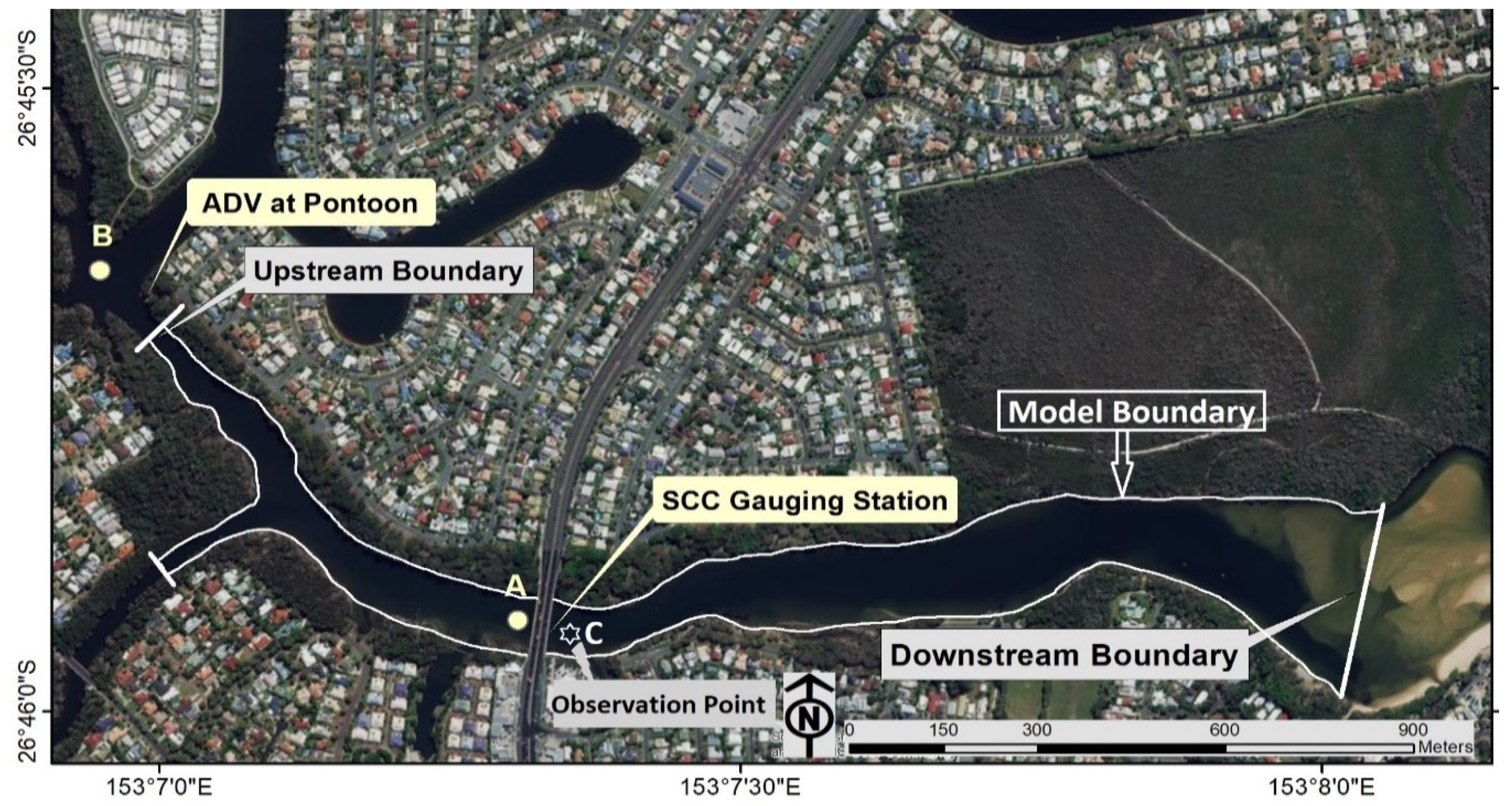
In this research, we focused on improving the accuracy of hydrodynamic modelling of estuaries using combined Eulerian and Lagrangian datasets. The current work was conducted in Currimundi Lake, (Longitude 153°08′10″ E, Latitude 26°45′40″ S) (Figure 1), a coastal lagoon located on Queensland’s Sunshine Coast. The estuary is classified within the context of Intermittently Closed and Open Lakes and Lagoons (ICOLLs) and is significantly affected by urbanization, recreation, environmental, social, and economic activities like many other Australian estuaries.
Using field data collected during open conditions in Currimundi Lake, we aimed at (i) evaluating the agreement between fixed-position instrumentation (Eulerian) and drifter (Lagrangian) velocity measurements in the channel, (ii) calibrating the hydrodynamic model (Delft3D FM) for Currimundi Lake using Eulerian and Lagrangian datasets via an automatic calibration methodology, and (iii) evaluating the improvement in model accuracies for the Lagrangian and Eulerian datasets. This paper is organised as follows: the materials and methods which include study area, field experiment, instrumentation, data analysis and hydrodynamic model setup are described in Section 2. A comparison between observed Lagrangian drifter and Eulerian ADV velocities in addition to a description of the calibration and validation procedure and results are presented in Section 3. In Section 4, we discuss the effects of Lagrangian calibration on hydrodynamic model accuracy, followed by a conclusion in Section 5.
2. Materials and Methods
2.1. Study Area
The field study location, Currimundi Lake main channel, during an open inlet condition is considered a micro-tidal estuary characterized by a semi-diurnal tidal pattern with a maximum spring tide of 0.8 m. The depth of the channel in mid-estuary varies between 3–5 m while the width varies between 300 m at the mouth and 70 m near the Pontoon (Figure 1). Freshwater discharges into Currimundi Lake system through Lake Kawana via a weir located 3.6 km from the channel inlet. The average discharge rate is 80 ML/day when the mouth is open. Since 1960, Currimundi Lake catchment area has experienced changes in land use becoming significantly urbanized and a center for recreational activities and fishing [26,30]. The Currimudi Lake main channel is connected to the ocean and upstream is fed by a constructed canal water body and tributaries (Figure 1). There is a connection to Lake Kawana via a weir, which is located 0.65 m above the AHD. A pumping regime of 1.8 ML/day from Mooloolah River into Lake Kawana and then into Currimundi Lake also contributes to ensure that water quality in the canal system is maintained [31].
2.2. Field Experiment Descriptions and Instrumentation
The field experiment was undertaken for 21 h during both ebb and flood conditions (27–28 April 2015) along the 2 km, relatively straight channel reach, downstream of the pontoon (Figure 1). The key forcings during an open condition for Currimundi Lake are wind, tide and discharge. These conditions varied during the 21-h experiment (Table 1). The field experiment focused on obtaining the flow velocity at the near surface using GPS-tracked floating drifters and fixed ADV.
Lagrangian drifters used in this study are low cost, made of PVC cylindrical pipes with 4 cm diameter and 50 cm length. The drifters design [18] contained off-the-shelf Holux GPS data loggers with absolute position accuracy between 2–3 m and were sampled at 1 Hz. A flock of 18 drifters were deployed in Currimundi Lake on 28 April 2015 in clusters of four at flood tide around 13:00 on 28 April and retrieved at around 16:00 the same day; two drifters were lost and two experienced logging errors. Drifter deployments were undertaken during a flood tide within the straight section of the channel between the bridge and pontoon (points A and B in Figure 1). Velocities were measured with a SontekTM 3D side-looking probe micro-ADV (16 MHz).The ADV was mounted 0.5 m below the water surface at the pontoon (B) and sampled continuously at 50 Hz during the 21 h period from 19:00 on 27 April to 16:00 on 28 April (Figure 2).
2.3. Quality Control and Data Analysis
The ADV data sets were quality-controlled and postprocessed to remove communication errors. Data points with correlations <60% and signal-to-noise ratios <5 dB were removed [32,33]. The drifter position data were quality controlled using velocity and acceleration de-spiking. Drifter positions with velocities >0.4 m/s were removed using a threshold of at least twice the expected peak velocity based on the previous flow history [23,34]. Sections of the trajectories where the drifters were trapped near banks or affected by proximity to moving objects, like boats, were removed using MATLAB scripts and experimental event logs. Unfiltered drifter data are not suitable for measuring small-scale processes in low flow applications because of the inherent position error that manifests as a large speed variance (σ2 ~ 0.0005 m2 s−2) in stationary tests at frequencies F>0.01 Hz. Therefore, position time series were low-pass filtered with a cut off frequency of Fc = 0.01 Hz.
2.4. Model Setup
2.4.1. Hydrodynamic Model
The hydrodynamic model for Currimundi Lake was developed using Delft3D FM, which has been widely used in coastal, river, and estuarine environments [35,36,37,38,39]. This multi-dimensional (2D or 3D) model is able to solve the Navier–Stokes equations for an incompressible fluid, under the shallow water equations and the Boussinesq assumptions [40]. The shallow water equations are derived from the Navier–Stokes equations assuming depth averaging and hydrostatic pressure distributions [41]. During the open condition of the entrance, salinity measured by the Sunshine Coast Council (SCC), varied between 25 and 33 g/l and tends to be well mixed vertically over large parts of the lake, which further justifies the use of a 2D model for the area of interest.
Calculations are performed in each cell using a cell-centred finite volume method. D-Flow FM uses an explicit advection scheme, which means the movement of an advected quantity is strictly limited to one grid interval in one-time step. To ensure the numerical stability of the explicit solver, the time step size of the model (∆t) is calculated automatically by the computational kernel, such that the maximum allowed Courant number is 0.7, the value advised in Delft3D FM manual. The Courant number represents the spacing portion of a grid cell that a flow passes through in one-time step. In vertically averaged simulations, dispersion is not simulated because the vertical profile of the horizontal velocity is not resolved, but dispersion can be modelled as a viscosity coefficient and a velocity gradient [40]. Horizontal eddy viscosity is held uniform throughout the domain of interest, specified at a value of one based on a default setting in Delft3D FM manual. For bed roughness, a Manning’s coefficient equivalent to 0.023 was specified in the first model simulation, selected based on the bed material surveyed in the main body of Currimundi Lake [42]. This value falls within feasible ranges of roughness parameters based on the literature [43,44]. Being in the middle of a sensible range, this value is chosen to be large enough to compensate for the model errors–mostly bathymetric errors–throughout the calibration. In the calibration process, Manning’s coefficient is adjusted to achieve the best match between modelled and observed measurements.
2.4.2. Flow Grid and Bathymetry
An unstructured, curvilinear finite-element grid was developed following the channel morphology with a relative high-resolution average grid of 5 m at the study site (Figure 1). To ensure that the model output was independent of the grid resolution, a grid independency test was performed. Five different grids were constructed in the minimum size range from 25 m down to 2 m. The cross-sectional average velocity at the middle of the domain (Point C in Figure 1) was used to examine the mesh convergence. The velocity was chosen in lieu of water level because the water level measured via a gauging station (Figure 1) was used for the downstream boundary condition. Results showed that the average velocity was not sensitive to further refinement beyond a minimum grid size of 5 m. However, an increase in the minimum grid size caused an increase in the cross-sectional average velocity. The bathymetry for the model to cover the model domain of interest was a LiDAR 5 m dataset [45], which had the highest coverage in the area of interest compared to the acoustic and manual bathymetry available at the time of this experiment. However, due to the uncertainties associated in LiDAR bathymetry that cause potential bias, a bathymetry correction process was undertaken in Section 3.2.1. A uniform roughness parameterised using Manning’s coefficient, n, was assumed throughout the domain, and hence a constant value was adopted for each simulation.
2.4.3. Model Forcing and Boundary Condition
The area of focus for this work was the main channel of Currimundi Lake, which is directly connected to the ocean through a tidal inlet. The modelled domain extends from this inlet to about 2 km upstream of the channel (Figure 1). The model is forced using discharge for the upstream boundary and water level at the downstream boundary. The discharge data were obtained from cross-sectional averaging of the ADV measurements at the pontoon and the water level data were obtained from the tidal gauging station at the bridge, approximately 1 km upstream from the boundary located at the mouth (Figure 1). The model time window was 21 h from 19:00 on 27 April to 16:00 on 28 April. A spin up time of 21 h including one high and two low tides was included for a realistic initial condition propagation.
Currimundi Lake is characterized by a small tidal range from 0.4 to 0.6 m. The discharge in the lake ranges between 0.15–30 m3/s as a function of the tidal phase while the depth ranges between 4.2 m– 0.15 mAHD. With the restricted model domain extent, there was a need to compare the contributions of the unmodeled sections of the Currimundi Lake to the hydrodynamics of the main channel. The percentage by volume of the water contribution from the unmodeled sections of the Currimundi Lake was estimated to be 16%. The comparison between the model results with and without the addition of 16% discharge from the South-West channel showed no discernible difference in velocities and water levels in the main channel. In addition, the total rainfall within the catchment seven days prior to the field measurements used in the study was less than 10 mm, thus, the stormwater runoff was assumed insignificant [26]. The input from the unmodelled section was therefore assumed negligible and ignored in the model.
3. Results and Discussion
3.1. Comparison and Correlation Analysis: Lagrangian and Eulerian Measurements
3.1.1. Comparison
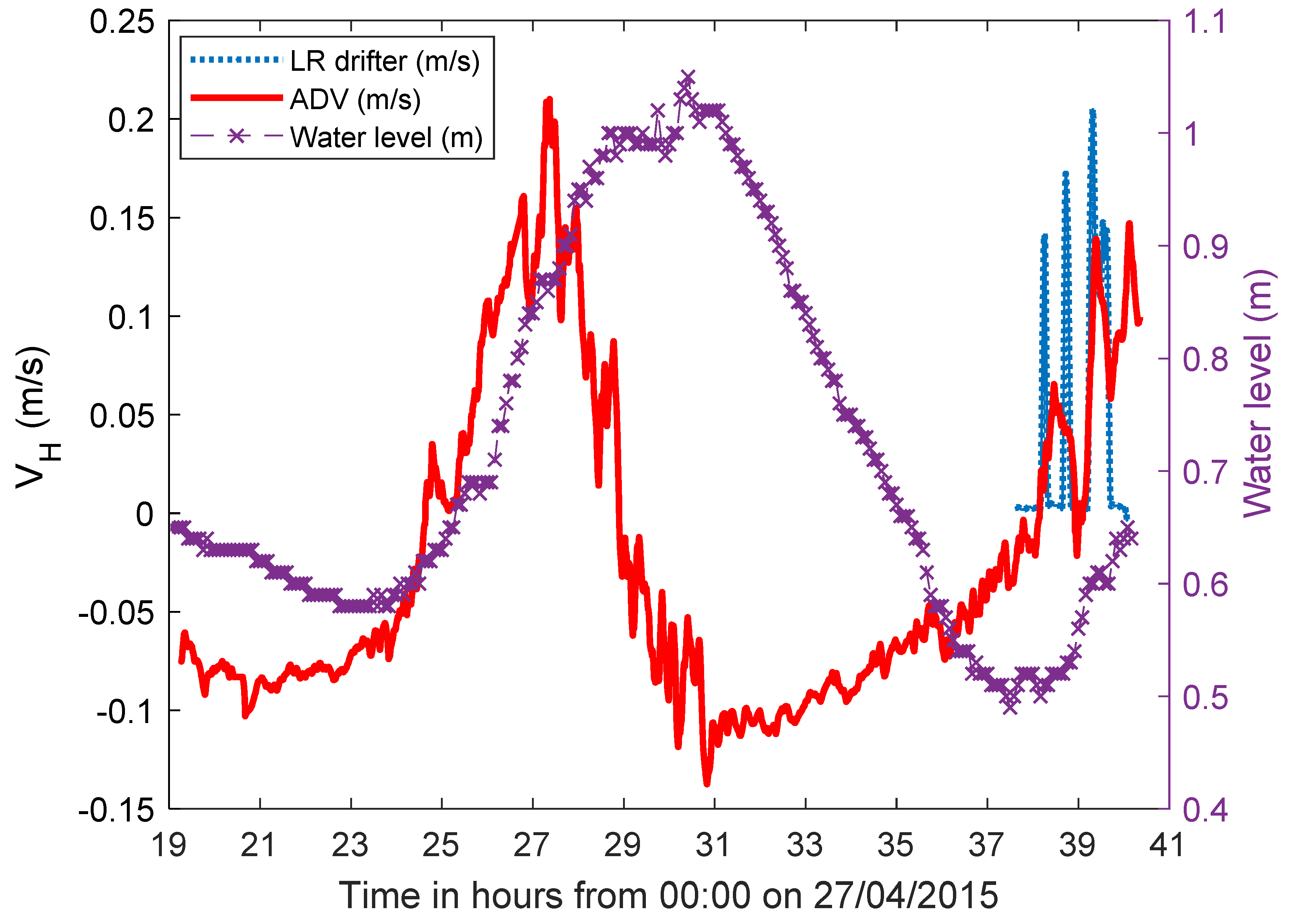
The temporal variability of mean horizontal velocity measured by the ADV is presented in Figure 3. A 200 s interval moving average was applied to the entire dataset; the moving average interval was chosen based on work by Chanson et al. [46] in a similar estuary. The surface water velocity collected by drifters during the experiment covered an area from 1000 m downstream to ~200 m upstream (from A to B in Figure 1) of the fixed instrument (ADV).
Both the drifter and ADV data captured the tidal scale fluctuation and the oscillation of the velocities at time periods less than the tidal period, likely related to the resonance within the channel. The drifter velocities are relatively higher than ADV velocities during peak flows and the reverse during the slack water. These larger flow velocities are likely related to the combined contribution of the large surface current and wind-induced surface current flows and cannot be captured by the ADV, which is a point measurement placed 0.5 m above the water surface. On the other hand, the slack periods had velocities, which were approximately zero, which were within the noise level of the drifter when evaluated from stationary tests [23]. In addition, slack water is typically characterized by low frequency eddies with frequencies >0.01 Hz larger than the useful frequency range of the drifters [23]. This limitation of drifters at such low velocities has been highlighted in previous studies [17]
3.1.2. Correlation Analysis
The field experiment was designed so that all drifters passed through the transect where the ADV was installed allowing a correlation comparison of the Lagrangian-drifter velocity with the Eulerian-fixed position velocity measurements. For each drifter release, the drifter mean horizontal Lagrangian velocity (VL) was an average of all velocities from those drifters that passed within a specific radius (r) of the ADV at a specific time interval. Therefore, the velocities from multiple drifters that passed through the ADV could contribute to VL.
To investigate the correlation that exists between drifter-mean Lagrangian (VL) and Eulerian (VE) horizontal velocities, VL and VE were calculated at different proximities from the ADV. To properly describe the flow field, a spatial binning was undertaken for drifter observations. Considering the streamwise velocity, which is positive in the upstream direction, we examined this correlation in bins with a radius varying from 20 to 100 m. The streamwise velocity was obtained following the work in Suara et al. [23].
To ensure the mean velocity in each bin was statistically stable, we calculated the degrees of freedom (DoF), which measures the number of independent measurements, for each bin. A minimum of five DoF is required for statistical stability [47,48]. For Lagrangian data where consecutive measurements are not necessarily independent, DoF is calculated as a function of data density in a bin, i.e., product of the number of drifters and the average time each drifter spends in a bin, normalised by the decorrelation time scale, i.e., eddy turnover time. Following [47], the DoF can be calculated from Equation (1):
where j denotes each individual drifter, TT is the time each drifter spends inside an individual bin, and TL is the Lagrangian integral time obtained from calculating the ensemble average of the auto-covariance function of Lagrangian velocity [47,48]. Here, TL is approximately 20 s, according to [48] in a small estuary. Thus, 100 s of drifter data within each bin is required to meet the minimum five DoF criterion to be statistically significant.
The Eulerian velocity (VE) corresponding to (VL) is calculated as the time averaged over the period the drifters were within the specific radius of the ADV.
where Vi is instantaneous ADV velocity, and t1, t2 are the entering and departing times of drifters corresponding to VL.
A sensitivity analysis was undertaken to obtain the optimum radius (r). The criteria used in the sensitivity analyses were a DoF ≥5 with the greatest number of independent data points. The radius (r) varied from 60 m down to 5 m and the optimum radius was determined to be 20 m with an R2 = 0.76 (Figure 4). Increasing r to 40 m resulted in R2 = 0.72. However, reducing r to 10 m, reduced the number of points required to meet the DoF ≥5 constraint without improving the linear regression.
Cross stream velocities of the drifters (VL) and the ADV (VE) were rather poorly correlated with the drifter velocities larger than ADV velocities (Figure 4). Some of the disagreements between Eulerian velocity (VE) and Lagrangian velocity (VL) may be related to: (i) The difference in Eulerian and Lagrangian instrument sampling location: the ADV measures water velocity 0.5 m below the surface while the drifters measure surface velocity. Because water profiles in wide open channels follow power law functions, we corrected the ADV velocities by applying a power law for uniform equilibrium flows in a wide-open channel. (ii) The difference in sampling volumes: the small sample volume of the ADV responds faster to the underlying flow field compared to the larger sample volume of drifters, which acts as a filter and is not able to capture small fluctuations. The small control volume of ADV impairs the insight into spatial structures and dynamics of the flow [49,50] and requires the application of considerable units of ADV [51]. (iii) Wind-induced surface flow effects on the drifters: drifters are more responsive to the surface flow velocities induced by the wind while the ADV captures the velocity of subsurface layers. (iv) Wind-induced slip of the drifters: approximately 30-mm unsubmerged height of each drifter is exposed to direct wind drag resulting in the horizontal motion of the drifter, which is dissimilar to the current motion [52]. The wind effect could impact the path and velocity of the drifter. This effect could not be eliminated and should be considered in drifter applications particularly in low velocity environments.
3.2. Model Calibration
Herein, the calibration of the hydrodynamic model was undertaken with two categories of datasets and was therefore categorised into two parts: Eulerian calibration using velocity measurements collected from a fixed-instrument (ADV) and Lagrangian calibration using velocities from GPS-tracked drifters. Both methods were based on an error criterion and correlation between observed and simulated velocities and were mainly used to fine tune the bed roughness coefficient through the Manning’s coefficient (n) [53,54]. Although the Eulerian calibration [55,56] is still used for hydrodynamic models, it is limited to sections of the water body and only reflects discrete information of flow hydrodynamics. This limitation can be improved with a larger observation density to represent the flow condition over a large area, which can be obtained from Lagrangian datasets. To investigate how the Lagrangian calibration improves model performance, we calibrated and tested the model with Eulerian and Lagrangian data separately. During the calibration process, the root-mean-square error (RMSE) of the observed Eulerian velocity (Vobs) versus Delft3D FM model velocity (Vsim) was minimized to identify an estimate of uncertain bathymetry and the roughness parameter [57] (Equation 3).
where Vsim is the model velocity, Vobs is the measured velocity, and n is the total number of measurements.
3.2.1. Bathymetry Correction
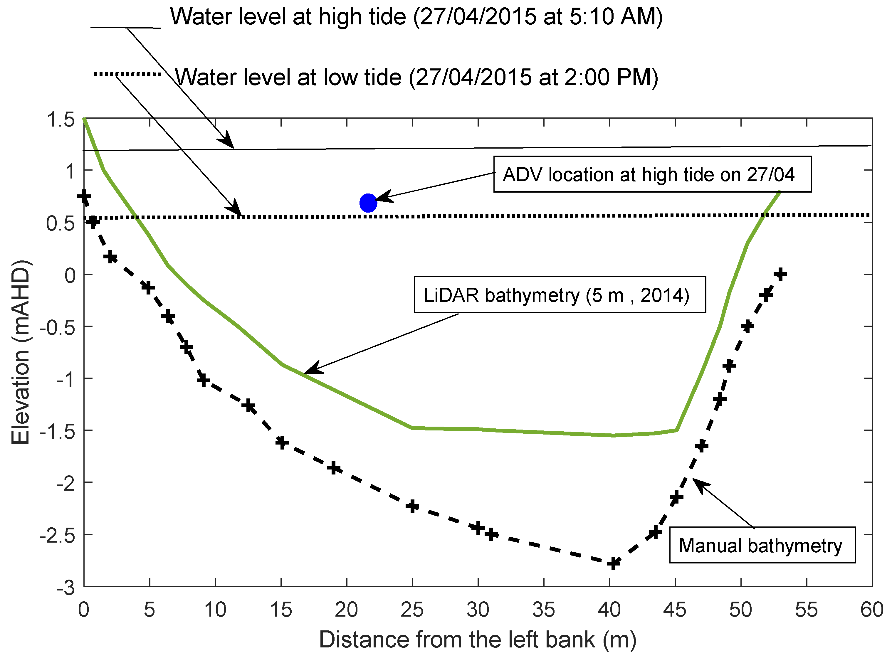
In most hydrodynamics models of estuaries, the pivotal calibration parameter is the bottom roughness coefficient [58,59]. This is because there are high levels of uncertainties associated with the estimation of bed friction from observational data [60]. However, the velocity field in estuaries is highly dependent on the variation of the cross-sectional areas, which is dictated by the bathymetry, especially in intertidal zones of shallow waterbodies [61,62]. Measurement uncertainties from different survey techniques, systematic offsets due to datum differences, and channel morphology evolution are major sources of error in bathymetry [53,63]. Therefore, prior to calibrating the hydrodynamic model based on bed friction, we first quantified the uncertainties associated with the hydrodynamic model output due to these bathymetric errors. The comparison of the LiDAR 5 m bathymetry data with the manual measurements at selected cross sections showed that the LiDAR data were offset about 0.75 m above the manual measurements (Figure 2) throughout the channel. The manual bathymetry survey was undertaken in 2015 by our team. A manual technique was employed using a staff gage and rope. Three sections were compared but only one is shown here. In addition to manual surveyed transects, we compared two transects from the main body of Currimundi lake with the LiDAR bathymetry. The surveyed section of the main body of Currimundi lake extended from the mouth (the lake and ocean intersection) up to 1 km upstream of the channel and was surveyed with a multibeam echo sounder in 2015. The positioning accuracy (horizontal and vertical) for this survey data was 1–2 cm. Comparing the accuracy of manual and acoustic bathymetry to the LiDAR dataset, the first two were considered accurate. We then corrected the LiDAR dataset to remove the bias while the manual and acoustic data were considered as the ground truth. The bathymetric correction process was validated, and the offset was found to be consistent with the difference between the LiDAR and the ground truth at all locations where acoustic and manual measurements were available. Therefore, a valid bathymetry was utilized in the model to further investigate the objective of calibrating the hydrodynamic model by adjusting Manning’s coefficient. Because the channel was reasonably sheltered and the tide was the major forcing during the open inlet condition in Currimundi Lake, [26] the only model parameter for the calibration process was the roughness. This was consistent with practices in literature where obtaining improved flow velocities is the goal [64].
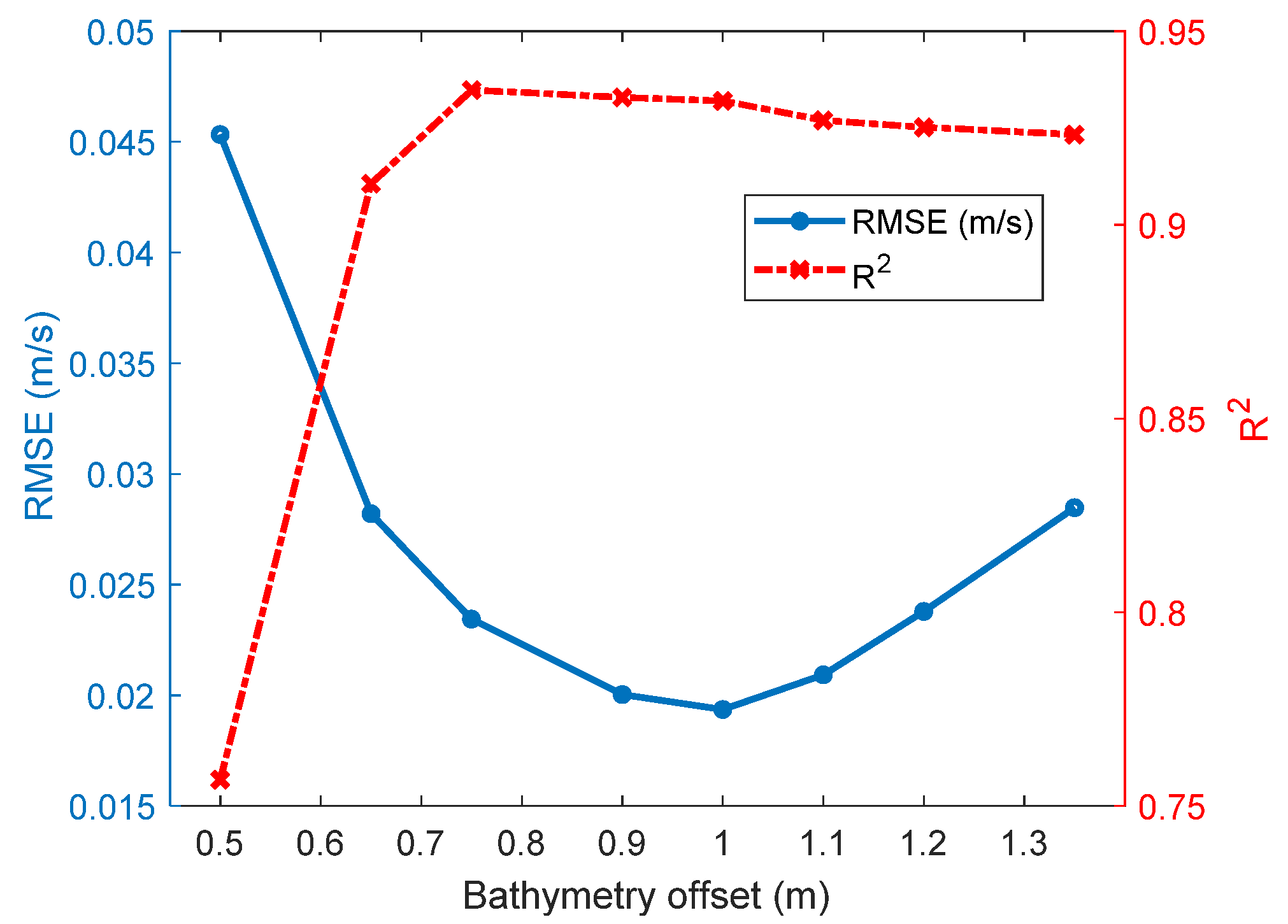
Simulations are run with a systematic bathymetry data offset in a sensible range of 0.5–1.3 m, guided by the offset observed between LiDAR and the manual measurements. A constant offset was applied across the domain to find the best agreement between the simulated and observed Eulerian velocities. Using the optimised bathymetry, a further calibration was applied by fine tuning Manning’s coefficient. This was undertaken using n = 0.01–0.03 based on [65]; this range was used to represent a roughness from firm soil to gravel bed material, which are representative substrates in Currimundi Lake.
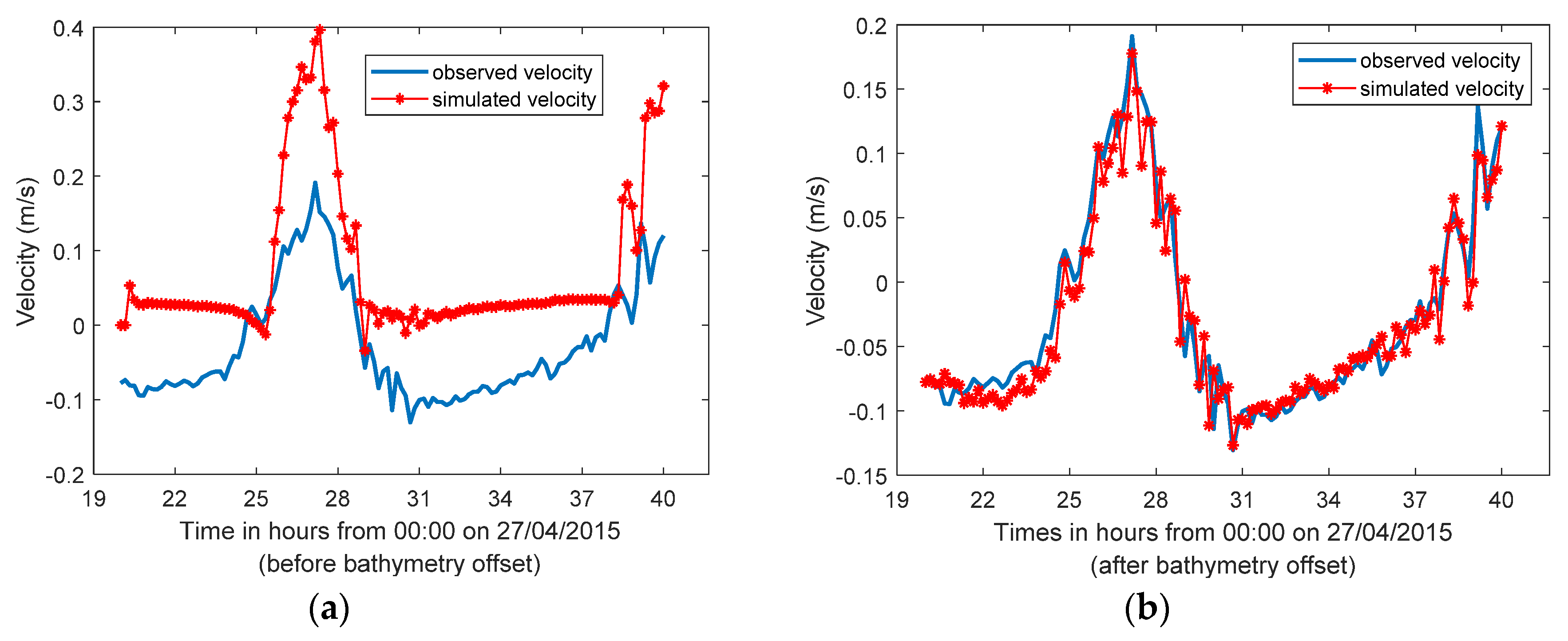
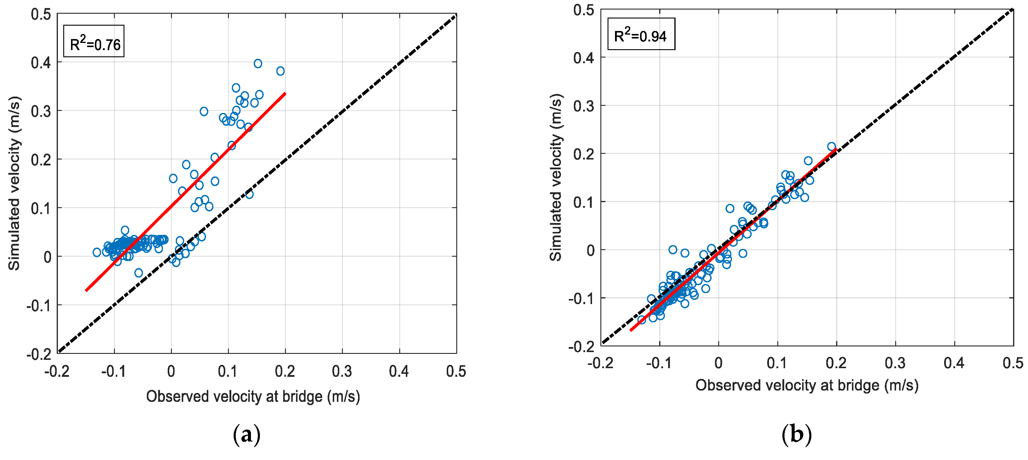
Figure 5 shows the R2 and RMSE values between the model and ADV horizontal velocities for different values of bathymetry offset. The RMSE reached a minimum at ∆z = 1 m, while the R2 value had a maximum at ∆z = 0.75 m. Therefore, we conclude that an optimum bathymetry offset of 1 m is suitable to improve the model velocity in the system. The corresponding velocity time series before and after applying the bathymetry offset are shown in Figure 6 and the corresponding scatter plots are shown in Figure 7. Prior to the bathymetry offset, the amplitude of the simulated velocity was considerably higher than the observed velocity contributing a systematic error that could only be removed by bathymetry offset. It should be noted that an attempt was made to calibrate the model with Manning’s coefficient prior to the bathymetry offset, however, this did not obtain a plausible correlation between the simulated and observed velocities.
3.2.2. Eulerian Calibration
Further model improvement was achieved by adjusting the roughness coefficient for the entire lake. To allow independence between the calibration and validation, 70% of the data were allocated for calibration and 30% for validation. To optimize the roughness coefficient, the Manning’s coefficient (n) was altered while the bathymetry was kept constant at 1 m, the optimal bathymetry offset.
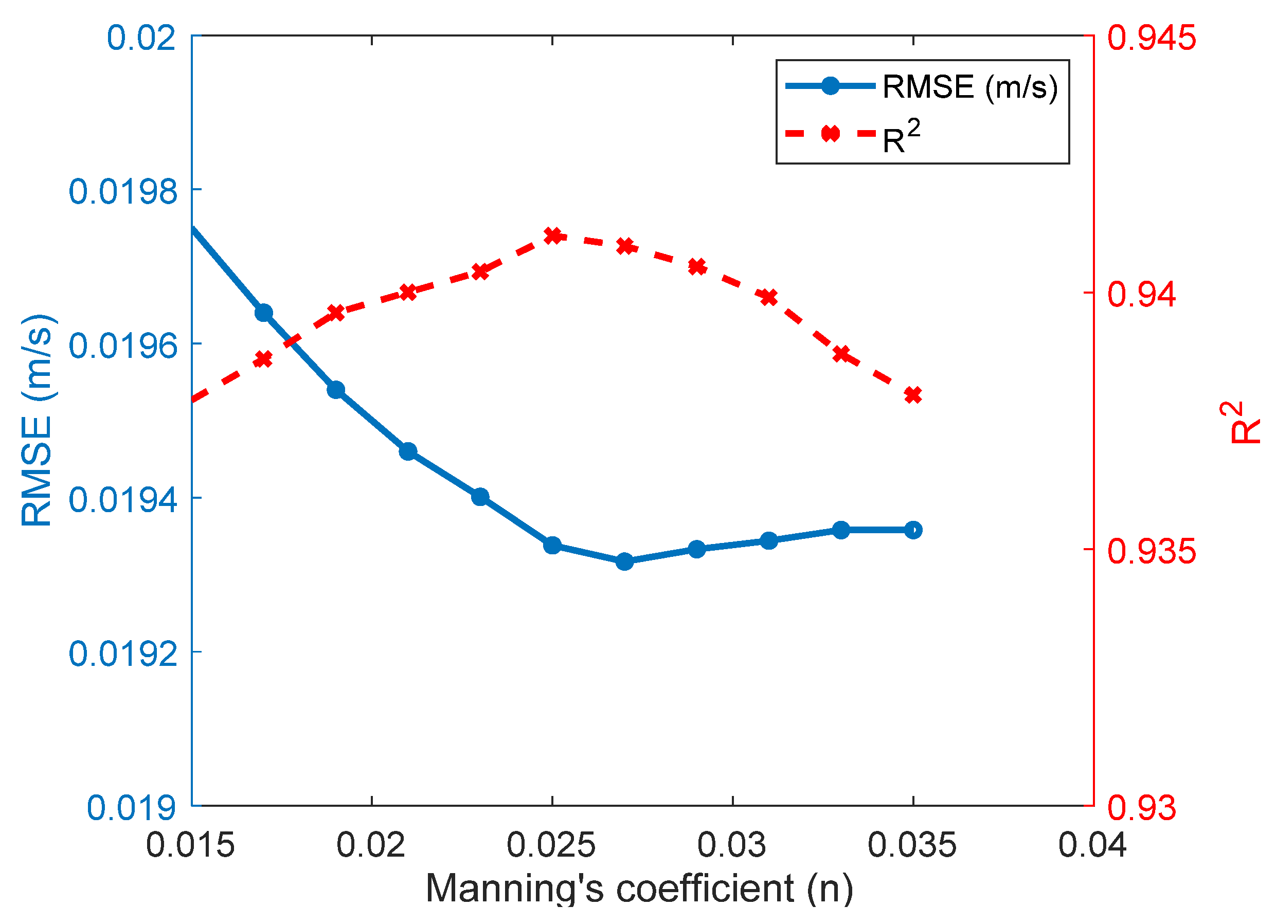
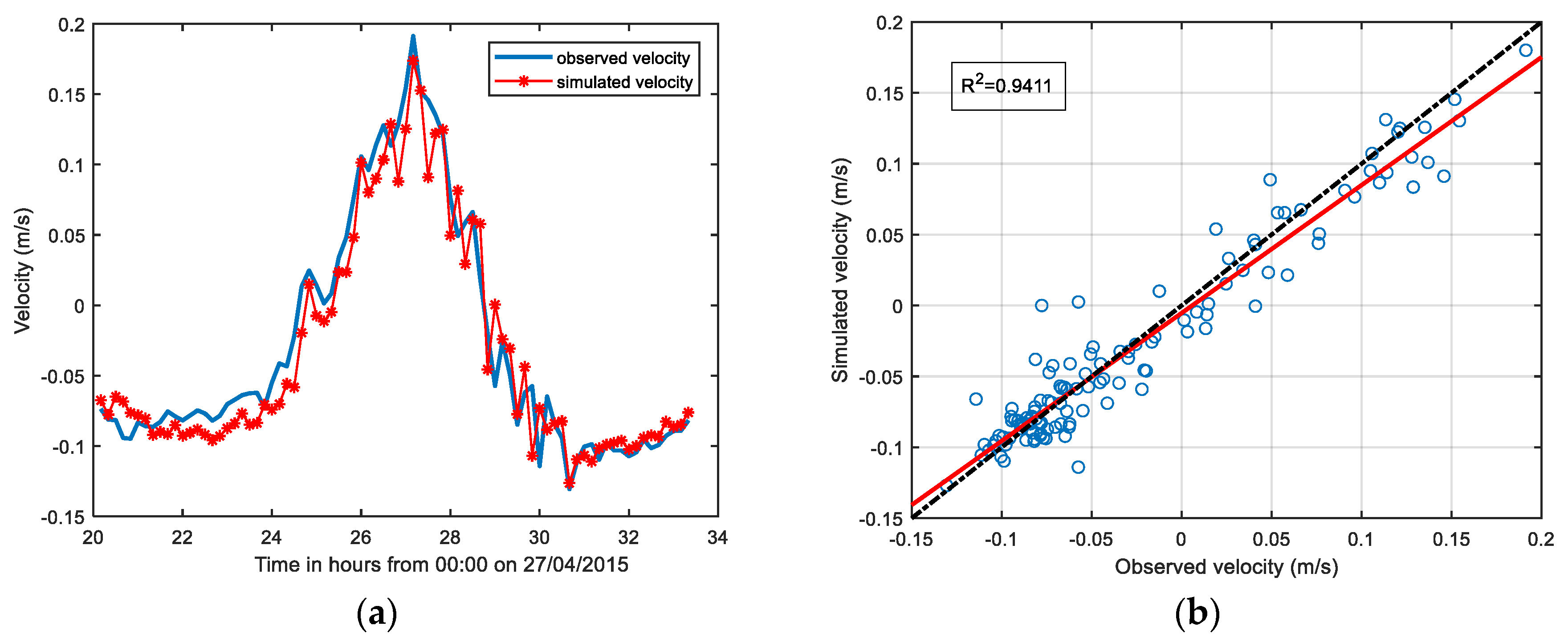
The result of the optimization is presented in Figure 8. The minimum RMSE (0.0193) was obtained at n = 0.027, while the R2 value reached a maximum (0.941) at n = 0.025. Based on the range of variation for both RMSE and R2 values, a Manning’s coefficient equal to 0.025 was selected as an optimum. Simulated and observed velocities were compared when n = 0.025 was applied. When comparing RMSE and R2 with n = 0.023 after optimum bathymetry offset (Figure 5), some improvement in the model resulted (Figure 8). Figure 9a and b shows a good agreement and correlation between simulated and observed velocities at n = 0.025, respectively, with 70% of the data.
3.2.3. Lagrangian Calibration
Difficulties in the calibration of Lagrangian data originate from the difference in the frame of reference. The model state is characterized by Eulerian variables, which are obtained from a fixed grid point. Here, we propose a method by which the hydrodynamic model is calibrated using Lagrangian drifter data. Lagrangian data collected during the field experiment are used as reference data for the calibration of the hydrodynamic model. Velocity data were obtained from a total of 16 drifters deployed within the domain of interest, 1 km from the mouth. Drifter trajectories in the main channel of Currimundi Lake on 28 April 2015 in flood condition when the mouth was open is shown in Figure 10.
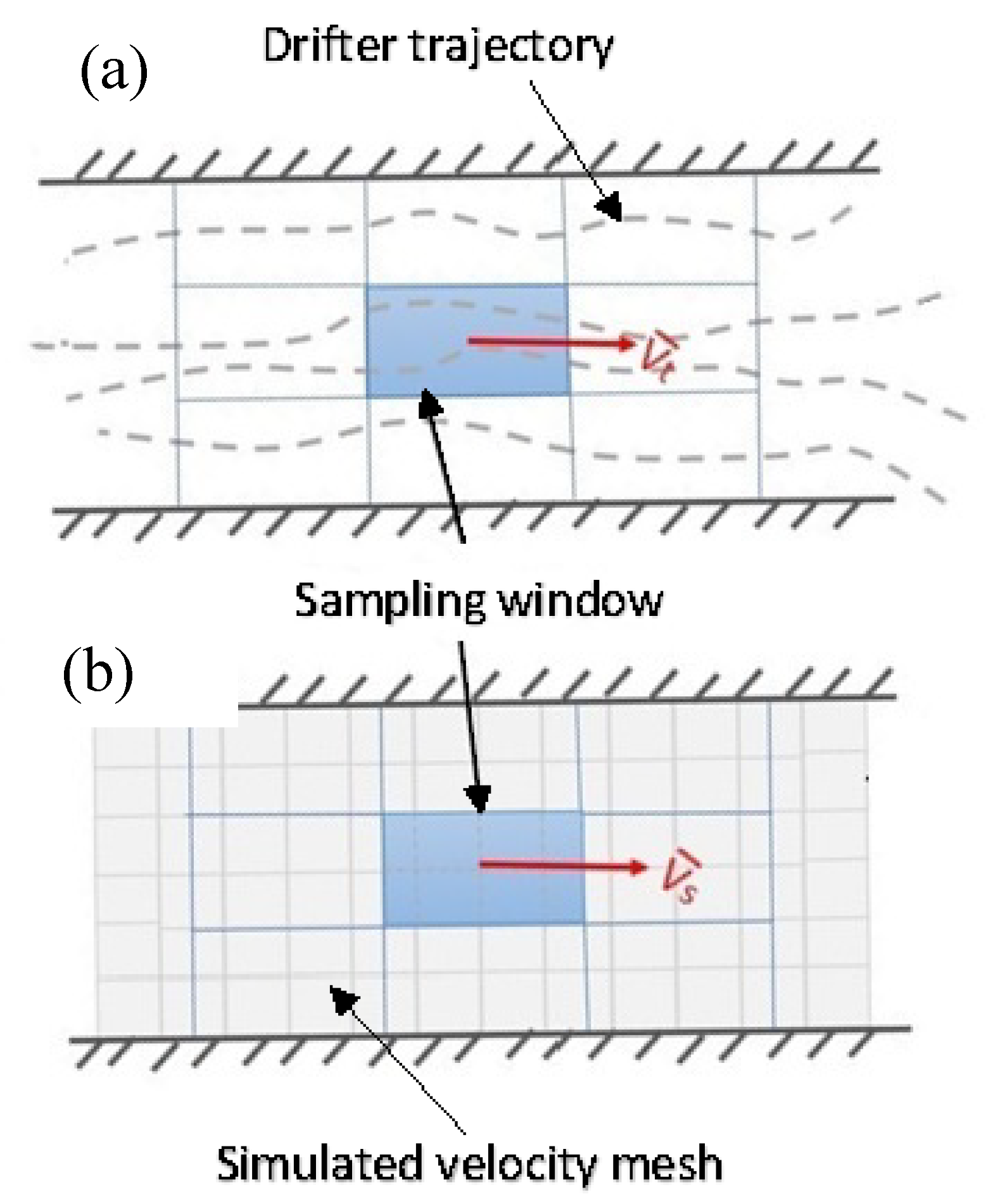
The drifter trajectories were recorded every second and postprocessed as discussed in Section 2.3. To allow quantitative comparison of the drifter data with the model velocities, a spatio-temporal binning of the drifter data was undertaken. All drifter data points were first binned into the model grids. As multiple trajectories can constitute elements falling into a single bin, all the drifters present in the model grids are then averaged to represent the mean Lagrangian velocity for each bin. The average of the times for the drifter velocity for each bin represent the observation time for the corresponding bin. It should be noted that not all model grids and times had an observation within this spatio-temporal binning (Figure 11).
To undertake Lagrangian calibration, an algorithm was developed in MATLAB that identified the optimum values of Manning’s coefficient through minimizing the difference between simulated and observed velocities using RMSE and R2 criteria. The calibration process iteratively alters Manning’s coefficient until the best possible adjustment between the simulated and the drifter velocities is achieved. The bathymetry used for calibration is the improved bathymetry (after 1 m offset). For calibration purposes, the velocity extracted from the model was compared to the corresponding depth-averaged velocity of the drifter location throughout the domain.
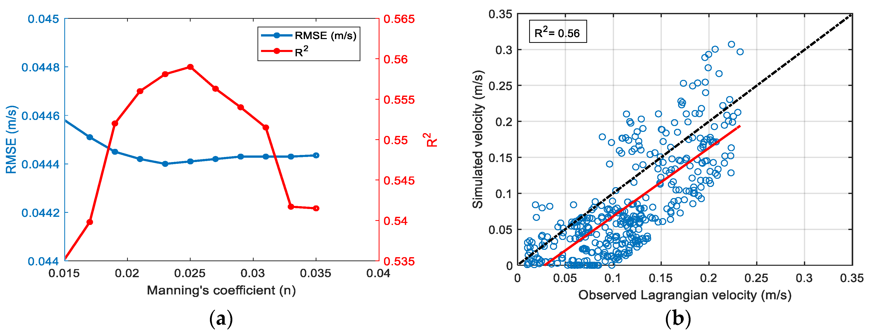
In Eulerian calibration, the best model performance was obtained with a Manning’s coefficient of 0.025 and the best correlation achieved when the Manning’s n = 0.025 was assigned (Figure 9b). Comparing the Eulerian calibration with Lagrangian calibration results, there was a slight difference in achieving an optimum Manning’s coefficient; the optimum Manning’s coefficient through Eulerian calibration is n = 0.025; for the Lagrangian calibration, the optimum coefficient was n = 0.023 (Figure 12a). On the other hand, the RMSE comparison between Eulerian and Lagrangian calibrations showed approximately 50% less improvement in the Lagrangian calibration (Figure 8 and Figure 12a). The correlation between observed and simulated velocities through Lagrangian calibration also shows about 40% less improvement in the results (Figure 8 and Figure 12b).
3.3. Model Validation
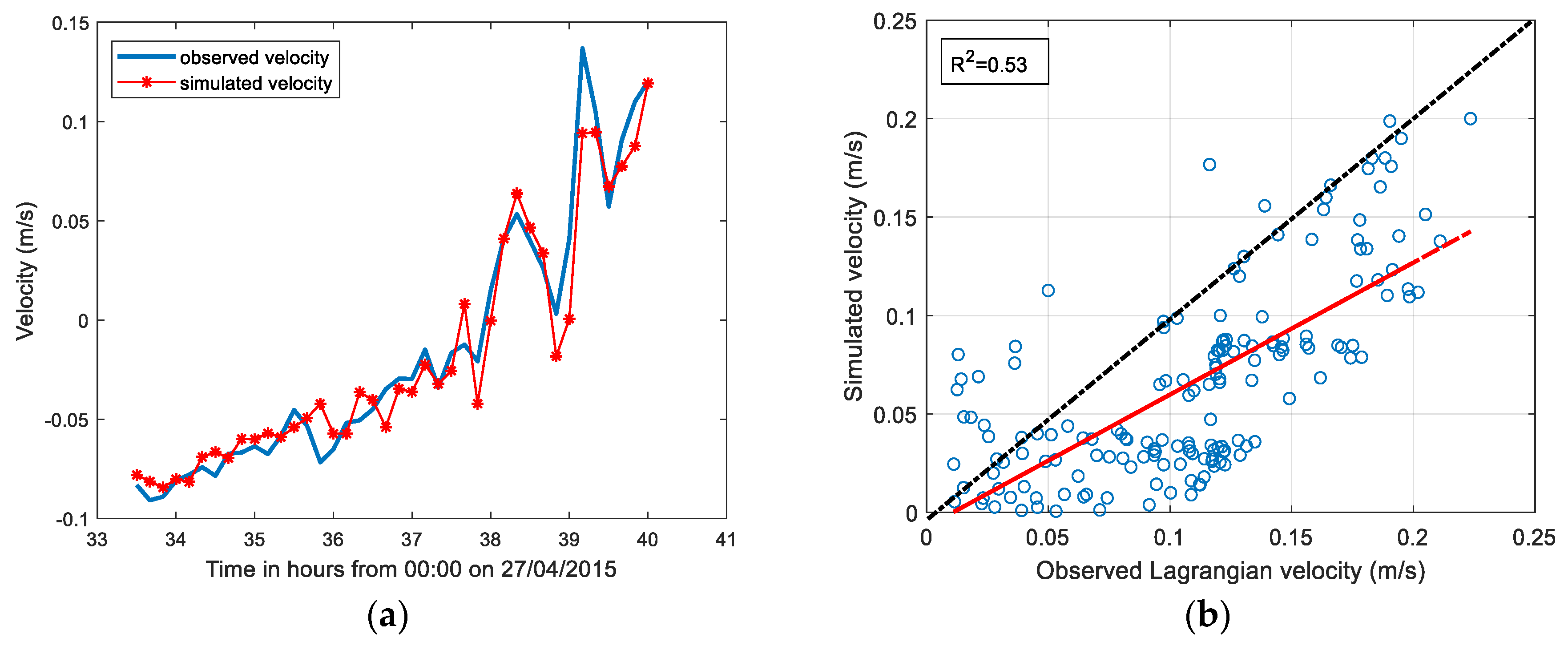
Our calibrated model was validated by comparing simulated velocities with 30% of the velocity measurements for both Eulerian and Lagrangian data. Based on the Eulerian calibration results in Section 4, the optimum Manning’s coefficient was n = 0.025. The Eulerian comparison between observed and simulated velocities is illustrated in Figure 13a. The RMSE and R2 calculated for this simulation was 0.014 m/s and 0.954, respectively, yielding a successful calibration and some improvement in model performance.
A corresponding Lagrangian validation was also undertaken by using 30% of the drifter velocity data when the model simulations used a Manning’s coefficient of n = 0.023 as noted in Lagrangian calibration (Section 4). The calculated RMSE and R2 criteria showed less improvement compared to the Eulerian validation results (Figure 13b). However, RMSE and R2 values for this simulation were 0.042 m/s and 0.53, respectively, which in comparison to the RMSE and R2 values for Lagrangian calibration (0.044 m/s and 0.56 respectively), reflected a successful calibration.
4. Discussion
A direct comparison between Eulerian derived (ADV) velocity and Lagrangian derived (drifter) velocity data was undertaken. The drifter observations had the best correlation in streamwise velocities with the ADV positioned next to the surface within a horizontal radius r = 20 m of the fixed ADV instrument. Consistent with this, Suara et al. [23] achieved a strong correlation between Eulerian and Lagrangian velocity measurements in the streamwise direction in a tidal estuary. Schmidt et al. [22] and Spydell et al. [17] found a very good correlation in the streamwise direction between the velocity measurements of drifters and a fixed-position instrument in a surf-zone and a tidal inlet, respectively. These findings highlight the potential in the use of Lagrangian field data to calibrate Eulerian-based hydrodynamic models. Figure 4 shows some disagreement between the Eulerian velocity measured by ADV and Lagrangian velocity measured by drifters. The large values of drifter streamwise velocity compared to ADV velocity can be explained by methodological and practical limitations that exist in the application of Eulerian and Lagrangian devices. These limitations include: (1) the differences in distances from the free surface water, which means that the drifters measure the surface velocity while the ADV measures the velocity in a corresponding depth; (2) the inability of the ADV to sample the spatial structure of a large volume in the domain; (3) the wind-induced currents, which affect the drifters more than the ADV; and (4) the inevitable wind drag effect on the unsubmerged height of the drifter. These restrictions are unavoidable and require attention when interpreting results of comparison between drifter and fixed Eulerian devices.
Eulerian and Lagrangian methods of calibration were applied using velocity time series data and GPS-tracked drifter velocities, respectively, and a comparison between Eulerian and Lagrangian calibration was established to investigate the effect of Lagrangian calibration on the hydrodynamic model improvement. The comparison showed both similarities and differences. Although, an optimum roughness was obtained, results here showed that for both calibrations, the sensitivity of the simulated velocity to bed roughness coefficient was low. This indicates that, in the case of Currimundi Lake, the velocity field is not very sensitive to errors in the imposed bed friction. RMSE and R2 variations calculated through the Eulerian method showed that the optimum Manning’s coefficient that minimized the error and maximized the correlation between observed and simulated velocity was in accordance with the one obtained through the Lagrangian method in the range of n = 0.023 to 0.025.
Considering the empirical uncertainties associated with calculating Manning’s roughness, the Lagrangian calibration method can be an alternative to the Eulerian method. This study showed that the correlation between the observed and simulated velocity was much higher when the model was calibrated using Eulerian time series velocity. However, the level of agreement between velocity values in Figure 8 and Figure 12a confirms that there are no discrepancies between the observed and simulated velocities. Some of the disagreements between observed and simulated velocities in the Lagrangian method of calibration can be justified based on the application of a two-dimensional model with vertically-averaged velocity, which is inherently different compared to the surface velocities of the drifters. The effect of wind drag, the submerged length of the drifter compared to the submerged length of ADV, and the different reference frame between drifters (Lagrangian frame) and the model (Eulerian frame) are also possible factors for disagreement between the observed and simulated values. The level of correlation observed between the drifters and the hydrodynamic model output (R2 = 0.56) was consistent with similar comparisons in other research. For example, the work of Huhn et al. [66] showed the correlation between drifters and modelled velocity in a tidal driven estuary with hourly position data, where R2 varied between 0.64 and 0.8 during four experiments. While in the work undertaken by Abascal et al. [67] in the coast of Spain with hourly averaged currents, the correlation observed was R2 =0.67 to 0.74. These levels of correlation are expected because the hydrodynamic model outputs represent a special mean velocity covering the minimum size of the grid (5 m) while drifters respond to higher frequency fluctuation. We performed a comparison of the model and drifters using two time average windows, 400 s and 800 s. The results showed that in comparison with the correlation observed using the 200 s window proposed in the paper, the correlation increased to R2 = 0.66 and R2 = 0.75 for 400 s and 800 s windows, respectively. This shows that the comparison improves when higher frequency values of the drifters are removed through averaging.
5. Conclusions
Generally, performance of a hydrodynamic model depends on two sources of information; first the properties of the system under simulation such as bed roughness, viscosity and bathymetry, and second, measurements of the system state, such as velocity and water level. In our calibration process, we adjusted the former until the agreement between the latter and the model results could be judged as “reasonably good”. However, as such, “prior information” of the system was generally associated with a certain level of noise and even when the model result is considered as a good match to measurements, it may have significant errors [68]. Furthermore, Tiedeman et al. [69] indicated that model calibration only cannot definitely decrease model uncertainties. Data assimilation, based on Bayes theorem incorporates these two sources of information into a ‘‘posterior parameter distribution’’ that defines both the limitation of the calibration process and knowledge of parameters that have not been “touched” in this process. Based on these considerations and findings, data assimilation is suggested as a tool by which the residual uncertainties associated with the two sources of information outlined above can be reduced further. Our results indicated a good model performance when Eulerian calibration was undertaken even without data assimilation. However, applying a data assimilation technique can favourably compensate for the discrepancies in model performance when Lagrangian assimilation is undertaken. Lagrangian data covers a wide range of spatio-temporal scales within the system and captures the underlying physical processes that cannot be captured by a hydrodynamic model. Therefore, the result of Lagrangian calibration here highlights that a Lagrangian data assimilation approach currently under investigation has the potential to further improve the accuracy of hydrodynamic models.
The results show that there is a higher level of correlation (R2 = 0.94) between model output and observed velocity data for the Eulerian calibration compared to that of Lagrangian calibration (R2 = 0.56). This lack of correlation between the model and Lagrangian data is a result of apparent differences between Lagrangian data and Eulerian (fixed-mesh) hydrodynamic model outputs. These differences can be due to the application of a two-dimensional, average velocity model, and the effects of wind-induced currents and turbulence in the flow. However, an increase in the correlation factor was detected when the time average window increased to 400 s and 800 s. Despite this, the results show that Lagrangian calibration resulted in optimum Manning coefficients (n = 0.023) equivalent to those observed through Eulerian calibration. Therefore, it is expected that through the application of a data assimilation methodology, the hydrodynamic model can be further improved using Lagrangian data.
Author Contributions
All authors (N.M., K.S., H.F., R.B., A.M. and R.C.S.) designed and performed the experiment. N.M. and K.S. analysed the data. N.M. wrote the manuscript. All authors interpreted the data, discussed and edited the manuscript. All authors have read and agreed to the published version of the manuscript.
Acknowledgments
The authors acknowledge the financial supports received from the Australian Research Council through Linkage grant LP150101172 as well as the Sunshine Coast Council for providing access to station data. The authors would also like to thank USC and QUT volunteer undergraduates, who participated in the field study.
Conflicts of Interest
The authors declare no conflicts of interest.
References
- Ganju, N.K.; Mark, J.B.; Brenda, R.; Alfredo, L.A.; del Pilar, B.; Jason, S.G.; Lora, A.H.; Samuel, J.L.; McCardell, G.; O’Donnell, J.; et al. Progress and Challenges in Coupled Hydrodynamic-Ecological Estuarine Modeling. Estuaries Coasts 2016, 39, 311–332. [Google Scholar] [CrossRef] [PubMed] [Green Version]
- Martin, J.L. Application of two-dimensional water quality model. J. Environ. Eng. 1988, 114, 317–336. [Google Scholar] [CrossRef]
- Liu, W.-C.; Hsu, M.-H.; Kuo, A.Y. Modelling of hydrodynamics and cohesive sediment transport in Tanshui River estuarine system, Taiwan. Mar. Pollut. Bull. 2002, 44, 1076–1088. [Google Scholar] [CrossRef]
- Karim, M.F.; Mimura, N. Impacts of climate change and sea-level rise on cyclonic storm surge floods in Bangladesh. Glob. Environ. Chang. 2008, 18, 490–500. [Google Scholar] [CrossRef]
- Sheng, Y.P. Evolution of a three-dimensional curvilinear-grid hydrodynamic model for estuaries, lakes and coastal waters: CH3D. In Estuarine and Coastal Modeling; ASCE: Reston, FL, USA, 1990. [Google Scholar]
- Spaulding, M.L.; Mendelsohn, D.L. WQMAP: An integrated three-dimensional hydrodynamic and water quality model system for estuarine and coastal applications. Mar. Technol. Soc. J. 1999, 33, 38–54. [Google Scholar] [CrossRef]
- Lane, S.; Richards, K.; Chandler, J. Developments in monitoring and modelling small-scale river bed topography. Earth Surf. Process. Landf. 1994, 19, 349–368. [Google Scholar] [CrossRef]
- Broomans, P.; Vuik, C. Numerical Accuracy in Solutions of the Shallow Water Equations. Master’s Thesis, Technical University of Delft, Delft, The Netherlands, 2003. [Google Scholar]
- Camacho, A.R.; Martin, J.L. Bayesian Monte Carlo for evaluation of uncertainty in hydrodynamic models of coastal systems. J. Coast. Res. 2013, 65 (Suppl. 1), 886–891. [Google Scholar] [CrossRef]
- Sørensen, T.J.V.; Madsen, H. Data assimilation in hydrodynamic modelling: On the treatment of non-linearity and bias. Stoch. Environ. Res. Risk Assess. 2004, 18, 228–244. [Google Scholar] [CrossRef]
- Serafy, E.Y.G.; Mynett, A.E. Improving the operational forecasting system of the stratified flow in Osaka Bay using an ensemble Kalman filter–based steady state Kalman filter. Water Resour. Res. 2008, 44. [Google Scholar] [CrossRef] [Green Version]
- van Sebille, E.; van Leeuwena, P.J.; Biastochb, A.; Barronc, C.N.; de Ruijtera, W.P.M. Lagrangian validation of numerical drifter trajectories using drifting buoys: Application to the Agulhas system. Ocean Model. 2009, 29, 269–276. [Google Scholar] [CrossRef] [Green Version]
- Döös, K.; Rupolo, V.; Brodeau, L. Dispersion of surface drifters and model-simulated trajectories. Ocean Model. 2011, 39, 301–310. [Google Scholar] [CrossRef]
- Zhang, A.; Parker, B.B.; Wei, E. Assimilation of water level data into a coastal hydrodynamic model by an adjoint optimal technique. Cont. Shelf Res. 2002, 22, 1909–1934. [Google Scholar] [CrossRef]
- Johnson, D.; Pattiaratchi, C. Application, modelling and validation of surfzone drifters. Coast. Eng. 2004, 51, 455–471. [Google Scholar] [CrossRef]
- Molcard, A.; Poje, A.C.; Özgökmen, T.M. Directed drifter launch strategies for Lagrangian data assimilation using hyperbolic trajectories. Ocean Model. 2006, 12, 268–289. [Google Scholar] [CrossRef]
- Spydell, M.S.; Feddersen, F.; Olabarrieta, M.; Chen, J.; Guza, R.T. Observed and modeled drifters at a tidal inlet. J. Geophys. Res. Ocean. 2015, 120, 4825–4844. [Google Scholar] [CrossRef]
- Suara, K.; Wang, C.; Feng, Y.; Brown, R.J.; Chanson, H.; Borgas, M. High-resolution GNSS-tracked drifter for studying surface dispersion in shallow water. J. Atmos. Ocean Technol. 2015, 32, 579–590. [Google Scholar] [CrossRef] [Green Version]
- Ferentinos, K.P.; Trigoni, N.; Nittel, S. Impact of drifter deployment on the quality of ocean sensing. In International Conference on GeoSensor Networks; Springer: Berlin/Heidelberg, Germany, 2006. [Google Scholar]
- Brocchini, M.; Calantoni, J.; Postacchini, M.; Sheremet, A.; Staples, T.; Smith, J.; Reedc, A.H.; Braithwaite, E.F.; Lorenzonia, C.; Russo, A.; et al. Comparison between the wintertime and summertime dynamics of the Misa River estuary. Mar. Geol. 2017, 385, 27–40. [Google Scholar] [CrossRef] [Green Version]
- Matte, P.; Secretan, Y.; Morin, J. Quantifying lateral and intratidal variability in water level and velocity in a tide-dominated river using combined RTK GPS and ADCP measurements. Limnol. Oceanogr. Methods 2014, 12, 281–302. [Google Scholar] [CrossRef] [Green Version]
- Schmidt, W.E.; Woodward, B.T.; Millikan, K.S.; Guza, R.T.; Raubenheimer, B.; Elgar, S. A GPS-tracked surf zone drifter. J. Atmos. Ocean Technol. 2003, 20, 1069–1075. [Google Scholar] [CrossRef]
- Suara, K.A.; Wang, H.; Chanson, H.; Gibbes, B.; Brown, R.J. Response of GPS-tracked drifters to wind and water currents in a tidal estuary. IEEE J. Ocean Eng. 2018, 44, 1077–1089. [Google Scholar] [CrossRef] [Green Version]
- Sawford, B.L.; Pinton, J.-F. A Lagrangian View of Turbulent Dispersion and Mixing, in Ten Chapters in Turbulance; Cambridge University Press: Cambridge, UK, 2013; pp. 132–175. [Google Scholar]
- Manning, P.J.; Churchill, J.H. Estimates of dispersion from clustered-drifter deployments on the southern flank of Georges Bank. Deep Sea Res. Part II Top. Stud. Oceanogr. 2006, 53, 2501–2519. [Google Scholar] [CrossRef] [Green Version]
- Suara, K.; Mardani, N.; Fairweather, H.; McCallum, A.; Allan, C.; Sidle, R.; Brown, R. Observation of the dynamics and horizontal dispersion in a shallow intermittently closed and open lake and lagoon (ICOLL). Water 2018, 10, 776. [Google Scholar] [CrossRef] [Green Version]
- Timms, B. Coastal dune waterbodies of north-eastern New South Wales. Mar. Freshw. Res. 1982, 33, 203–222. [Google Scholar] [CrossRef]
- Everett, D.J.; Baird, M.E.; Suthers, I.M. Nutrient and plankton dynamics in an intermittently closed/open lagoon, Smiths Lake, south-eastern Australia: An ecological model. Estuar. Coast. Shelf Sci. 2007, 72, 690–702. [Google Scholar] [CrossRef]
- Logan, B.; Taffs, K.H. Relationship between diatoms and water quality (TN, TP) in sub-tropical east Australian estuaries. J. Paleolimnol. 2013, 50, 123–137. [Google Scholar] [CrossRef]
- Sunshine Coast Council. Backward Glance: Changing Landscapes–Kawana. Available online: https://www.sunshinecoast.qld.gov.au/Council/News-Centre/Backward-Glance-Changing-Landscapes–Kawana (accessed on 5 June 2019).
- Tomlinson, R.; Williams, P.; Richards, R.; Weigand, A.; Schlacher, T.; Butterworth, V.; Gaffet, N. Lake Currimundi Dynamics Study Final Report Volume 1. (Research Report No. 75). Sunshine Coast, Australia; 2010. Available online: https://www.sunshinecoast.qld.gov.au (accessed on 1 June 2019).
- Chanson, H.; Trevethan, M.; Aoki, S.-I. Acoustic Doppler velocimetry (ADV) in a small estuarine system. Field experience and “despiking”. In Proceedings of the 31th Biennial IAHR Congress, Theme E2, Paper 0161, Seoul, Korea, 11–16 September 2005; Jun, B.H., Lee, S.I., Seo, I.W., Choi, G.W., Eds.; pp. 3954–3966. [Google Scholar]
- Brown, R.; Chanson, H. Turbulence and suspended sediment measurements in an urban environment during the Brisbane River flood of January 2011. J. Hydraul. Eng. 2012, 139, 244–253. [Google Scholar]
- Suara, K.; Brown, R.J.; Chanson, H. Turbulence and Mixing in the Environment: Multi-Device Study in a Sub-Tropical Estuary; School of Civil Engineering, The University of Queensland: Brisbane, Australia, 2015. [Google Scholar]
- Van Maren, D. Water and sediment dynamics in the Red River mouth and adjacent coastal zone. J. Asian Earth Sci. 2007, 29, 508–522. [Google Scholar] [CrossRef]
- Bouma, T.J.; Van Duren, L.A.; Temmerman, S.; Claverie, T.; Blanco-Garcia, A.; Ysebaert, T.; Herman PM, J. Spatial flow and sedimentation patterns within patches of epibenthic structures: Combining field, flume and modelling experiments. Cont. Shelf Res. 2007, 27, 1020–1045. [Google Scholar] [CrossRef]
- Tonnon, P.K.; Van Rijn, L.C.; Walstra, D.J.R. The morphodynamic modelling of tidal sand waves on the shoreface. Coast. Eng. 2007, 54, 279–296. [Google Scholar] [CrossRef]
- Allard, R.; Dykes, J.; Hsu, Y.L.; Kaihatu, J.; Conley, D. A real-time nearshore wave and current prediction system. J. Mar. Syst. 2008, 69, 37–58. [Google Scholar] [CrossRef] [Green Version]
- Harcourt-Baldwin, J.-L.; Diedericks, G. Numerical modelling and analysis of temperature controlled density currents in Tomales Bay, California. Estuar. Coast. Shelf Sci. 2006, 66, 417–428. [Google Scholar] [CrossRef]
- D-Flow Flexible Mesh User Manual. Manuals Delft3D FM Suite 2019. Available online: https://www.deltares.nl/en/software/delft3d-flexible-mesh-suite/ (accessed on 1 June 2019).
- Pokrajac, D. Depth-integrated Reynolds-averaged Navier–Stokes equations for shallow flows over rough permeable beds. J. Hydraul. Res. 2013, 51, 597–600. [Google Scholar] [CrossRef]
- Acoustic Imaging Pty Ltd. Currimundi Lake Survey-December 2015, Sunshine Coast Council. Australia. 2015. [Google Scholar]
- Werner, M.; Hunter, N.; Bates, P. Identifiability of distributed floodplain roughness values in flood extent estimation. J. Hydrol. 2005, 314, 139–157. [Google Scholar] [CrossRef]
- Fabio, P.; Aronica, G.; Apel, H. Towards automatic calibration of 2-D flood propagation models. Hydrol. Earth Syst. Sci. 2010, 14, 911–924. [Google Scholar] [CrossRef] [Green Version]
- Geoscience Australia. Digital Elevation Model (DEM) 5 Metre Grid derived from LiDAR. Available online: https://data.gov.au/organisations/org-ga-Geoscience%20Australia (accessed on 15 April 2019).
- Chanson, H.; Brown, R.; Trevethan, M. Turbulence measurements in a small subtropical estuary under king tide conditions. Environ. Fluid Mech. 2012, 12, 265–289. [Google Scholar] [CrossRef] [Green Version]
- MacMahan, J. Drifter Trajectories in Riverine Environments; Naval Postgraduate School, Oceanography Department, Spanagel 327c: Monterey, CA, USA, 2009. [Google Scholar]
- Suara, K.; Brown, R.; Borgas, M. Eddy diffusivity: A single dispersion analysis of high resolution drifters in a tidal shallow estuary. Environ. Fluid Mech. 2016, 5, 923–943. [Google Scholar] [CrossRef] [Green Version]
- Johnson, D.; Stocker, R.; Head, R.; Imberger, J.; Pattiaratchi, C. A compact, low-cost GPS drifter for use in the oceanic nearshore zone, lakes, and estuaries. J. Atmos. Ocean. Technol. 2003, 20, 1880–1884. [Google Scholar] [CrossRef]
- Schacht, C.; Lemckert, C. A new Lagrangian-Acoustic Drogue (LAD) for monitoring flow dynamics in an estuary: A quantification of its water-tracking ability. J. Coast. Res. 2007, 420–426, 26481625. [Google Scholar]
- Shaha, D.C.; Cho, Y.K.; Kwak, M.T.; Kundu, S.R.; Jung, K.T. Spatial variation of the longitudinal dispersion coefficient in an estuary. Hydrol. Earth Syst. Sci. 2011, 15, 3679–3688. [Google Scholar] [CrossRef] [Green Version]
- Lumpkin, R.; Pazos, M. Measuring surface currents with Surface Velocity Program drifters: The instrument, its data, and some recent results. Lagrangian Anal. Predict. Coast. Ocean Dyn. 2007, 39–67. [Google Scholar] [CrossRef]
- Cea, L.; French, J. Bathymetric error estimation for the calibration and validation of estuarine hydrodynamic models. Estuar. Coast. Shelf Sci. 2012, 100, 124–132. [Google Scholar] [CrossRef]
- Barker, J.; Pasternack, G.B.; Bratovich, P.M.; Massa, D.A.; Wyrick, J.R.; Johnson, T.R. Kayak drifter surface velocity observation for 2D hydraulic model validation. River Res. Appl. 2018, 34, 124–134. [Google Scholar] [CrossRef] [Green Version]
- Wasantha Lal, A. Calibration of riverbed roughness. J. Hydraul. Eng. 1995, 121, 664–671. [Google Scholar] [CrossRef]
- Becker, L.; William, W.-G. Identification of parameters in unsteady open channel flows. Water Resour. Res. 1972, 8, 956–965. [Google Scholar] [CrossRef]
- Legleiter, C.J.; Kyriakidis, P.C.; McDonald, R.R.; Nelson, J.M. Effects of uncertain topographic input data on two-dimensional flow modeling in a gravel-bed river. Water Resour. Res. 2011, 47. [Google Scholar] [CrossRef]
- Piedra-Cueva, I.; Fossati, M. Residual currents and corridor of flow in the Rio de la Plata. Appl. Math. Model. 2007, 31, 564–577. [Google Scholar] [CrossRef]
- Sousa, M.; Dias, J. Hydrodynamic model calibration for a mesotidal lagoon: The case of Ria de Aveiro (Portugal). J. Coast. Res. 2007, 1075–1080, 26481739. [Google Scholar]
- Li, C.; Valle-Levinson, A.; Atkinson, L.P.; Wong, K.C.; Lwiza, K.M. Estimation of drag coefficient in James River Estuary using tidal velocity data from a vessel-towed ADCP. J. Geophys. Res. Ocean 2004, 109, C3. [Google Scholar] [CrossRef]
- French, J. Hydrodynamic modelling of estuarine flood defence realignment as an adaptive management response to sea-level rise. J. Coast. Res. 2008, 24, 1–12. [Google Scholar] [CrossRef]
- Zheng, L.; Chen, C.; Zhang, F.Y. Development of water quality model in the Satilla River Estuary, Georgia. Ecol. Model. 2004, 178, 457–482. [Google Scholar] [CrossRef]
- Hare, R.; Eakins, B.; Amante, C. Modelling bathymetric uncertainty. Int. Hydrogr. Rev. 2011, 20888. [Google Scholar]
- Papanicolaou, A.; Elhakeem, M.; Wardman, B. Calibration and verification of a 2D hydrodynamic model for simulating flow around emergent bendway weir structures. J. Hydraul. Eng. 2011, 137, 75–89. [Google Scholar] [CrossRef]
- Chow, V.T. Open-Channel Hydraulics, in Open-Channel Hydraulics; McGraw-Hill: New York, NY, USA, 1959. [Google Scholar]
- Huhn, F.; von Kameke, A.; Allen-Perkins, S.; Montero, P.; Venancio, A.; Perez-Munuzuri, V. Horizontal Lagrangian transport in a tidal-driven estuary—Transport barriers attached to prominent coastal boundaries. Cont. Shelf Res. 2012, 39, 1–13. [Google Scholar] [CrossRef]
- Abascal, A.J.; Castanedo, S.; Medina, R.; Losada, I.J.; Alvarez-Fanjul, E. Application of HF radar currents to oil spill modelling. Mar. Pollut. Bull. 2009, 58, 238–248. [Google Scholar] [CrossRef]
- Moore, C.; Doherty, J. Role of the calibration process in reducing model predictive error. Water Resources Res. 2005, 41. [Google Scholar] [CrossRef] [Green Version]
- Tiedeman, C.R.; Hill, M.C.; D.’Agnese, F.A.; Faunt, C.C. Methods for using groundwater model predictions to guide hydrogeologic data collection, with application to the Death Valley regional groundwater flow system. Water Resources Res. 2003, 39. [Google Scholar] [CrossRef] [Green Version]
Figure 1.
Aerial view of Currimundi Lake catchment, main channel including ADV and drifter’s deployment locations, model boundary, observation point (C) and tidal gauge station; (map is created using ArcGIS software by Esri). Drifters were deployed at point A and retrieved at point B.
Figure 1.
Aerial view of Currimundi Lake catchment, main channel including ADV and drifter’s deployment locations, model boundary, observation point (C) and tidal gauge station; (map is created using ArcGIS software by Esri). Drifters were deployed at point A and retrieved at point B.

Figure 2.
Surveyed transect and 5 m, 2014 LiDAR bathymetry next to the pontoon near B (in Figure 1). The solid line is the water level at high tide at 5:10 a.m. and the dashed line is the water level at low tide at 14:00 on 27 April 2015.
Figure 2.
Surveyed transect and 5 m, 2014 LiDAR bathymetry next to the pontoon near B (in Figure 1). The solid line is the water level at high tide at 5:10 a.m. and the dashed line is the water level at low tide at 14:00 on 27 April 2015.

Figure 3.
Mean horizontal velocity for Eulerian (ADV) and Lagrangian (drifters) surface measurements as a function of time. Mean velocities were estimated by a moving average with a window size of 200 s.
Figure 3.
Mean horizontal velocity for Eulerian (ADV) and Lagrangian (drifters) surface measurements as a function of time. Mean velocities were estimated by a moving average with a window size of 200 s.

Figure 4.
Relationship between Lagrangian (VL) and Eulerian (VE) mean streamwise velocities in a 20 m radius.
Figure 4.
Relationship between Lagrangian (VL) and Eulerian (VE) mean streamwise velocities in a 20 m radius.

Figure 5.
Root-mean-square error (RMSE) and R2 variations against variation in bathymetry values show the optimum bathymetry offset.
Figure 5.
Root-mean-square error (RMSE) and R2 variations against variation in bathymetry values show the optimum bathymetry offset.

Figure 6.
Observed vs. simulated velocities (a): before 1 m bathymetry offset and (b) after 1 m bathymetry offset.
Figure 6.
Observed vs. simulated velocities (a): before 1 m bathymetry offset and (b) after 1 m bathymetry offset.

Figure 7.
Relationship between simulated and observed velocities: (a) before 1 m bathymetry offset and (b) after 1 m bathymetry offset.
Figure 7.
Relationship between simulated and observed velocities: (a) before 1 m bathymetry offset and (b) after 1 m bathymetry offset.

Figure 8.
RMSE and R2 criteria variation with respect to Manning coefficient alteration in Eulerian calibration.
Figure 8.
RMSE and R2 criteria variation with respect to Manning coefficient alteration in Eulerian calibration.

Figure 9.
Eulerian calibration: (a) Observed vs. Simulated velocity at n = 0.025, (b) correlation between observed and simulated velocity at n = 0.025.
Figure 9.
Eulerian calibration: (a) Observed vs. Simulated velocity at n = 0.025, (b) correlation between observed and simulated velocity at n = 0.025.

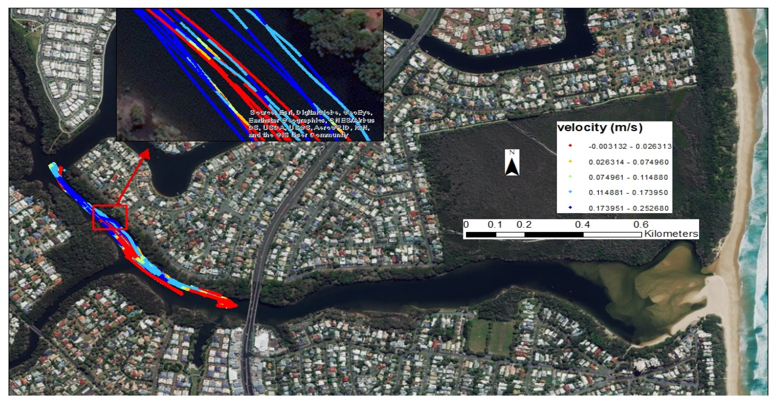
Figure 10.
Trajectories from 13:30 to 16:00 on 28 April 2015 with an open entrance and flood condition. Source: ArcGIS software by Esri.
Figure 10.
Trajectories from 13:30 to 16:00 on 28 April 2015 with an open entrance and flood condition. Source: ArcGIS software by Esri.

Figure 11.
Schematic spatio-temporal window of the domain. Grey dashed lines show the schematic drifter trajectories. The velocity arrow (Vl) in (a) denotes the mean velocity of drifters inside each cell, while the velocity arrow (Vs) in (b) denotes the mean simulated velocity obtained from the model in the same time frame.

Figure 12.
Lagrangian calibration: (a) RMSE and R2 variations against Manning’s coefficient iterations, (b) relationship between observed Lagrangian drifters and simulated velocities.
Figure 12.
Lagrangian calibration: (a) RMSE and R2 variations against Manning’s coefficient iterations, (b) relationship between observed Lagrangian drifters and simulated velocities.

Figure 13.
(a) Eulerian validation of the model by comparing the simulated and observed velocity using 30% of the data; (b) relationship between observed Lagrangian velocity and simulated velocity.
Figure 13.
(a) Eulerian validation of the model by comparing the simulated and observed velocity using 30% of the data; (b) relationship between observed Lagrangian velocity and simulated velocity.


Table 1.
Overview of the environmental conditions and instrumentation during the experiment.
| Inlet Condition | Date | Tide | Tidal Range (m) | Water Elevation (m) | Discharge Range (m3/s) | Wind Speed Range (m/s) | Instrument Deployed | Sample Frequency (HZ) |
|---|---|---|---|---|---|---|---|---|
| Open | 27/04/2015 | Ebb | 0.4 | 0.2 | 0.6–17 | 0–4.0 | ADV- Sontek-2D side-looking (16 MHz) | 50 |
| Open | 28/04/2015 | Flood/Ebb | 0.6 | 0.7 | 0.15–30 | 0–4.0 | LR drifters-Holux-GPS-tracked-specification: diameter: 4 cm height: 50 cm with ~47 cm submerged height | 1 |
© 2020 by the authors. Licensee MDPI, Basel, Switzerland. This article is an open access article distributed under the terms and conditions of the Creative Commons Attribution (CC BY) license (http://creativecommons.org/licenses/by/4.0/).
Share and Cite
MDPI and ACS Style
Mardani, N.; Suara, K.; Fairweather, H.; Brown, R.; McCallum, A.; Sidle, R.C. Improving the Accuracy of Hydrodynamic Model Predictions Using Lagrangian Calibration. Water 2020, 12, 575. https://doi.org/10.3390/w12020575
AMA Style
Mardani N, Suara K, Fairweather H, Brown R, McCallum A, Sidle RC. Improving the Accuracy of Hydrodynamic Model Predictions Using Lagrangian Calibration. Water. 2020; 12(2):575. https://doi.org/10.3390/w12020575
Chicago/Turabian StyleMardani, Neda, Kabir Suara, Helen Fairweather, Richard Brown, Adrian McCallum, and Roy C. Sidle. 2020. "Improving the Accuracy of Hydrodynamic Model Predictions Using Lagrangian Calibration" Water 12, no. 2: 575. https://doi.org/10.3390/w12020575
Note that from the first issue of 2016, this journal uses article numbers instead of page numbers. See further details here.