Impact of Deficit Irrigation on Shallow Saline Groundwater Contribution and Sunflower Productivity in the Imperial Valley, California

Abstract

Yield and production functions of sunflower (Helianthus annuus) were evaluated under full and deficit irrigation practices with the presence of shallow saline groundwater in a semi-arid region in the Imperial Valley of southern California, USA. A growing degree day (GDD) model was utilized to estimate the various growth stages and schedule irrigation events throughout the growing season. The crop was germinated and established using overhead irrigation prior to the use of a subsurface drip irrigation (SDI) system for the remainder of the growing season. Four irrigation treatments were implemented: full irrigation (100% full sunflower crop evapotranspiration, ET_C), two reduced irrigation scenarios (95% ET_C and 80% ET_C), and a deficit irrigation scenario (65% ET_C). The salinity of the irrigation water (EC) (Colorado River water) was nearly constant at 1.13 dS·m⁻¹ during the growing season. The depth to groundwater and groundwater salinity (EC_GW) were continuously monitored in five 3 m deep observation wells. Depth to groundwater fluctuated slightly under the full and reduced irrigation treatments, but drastically increased under deficit irrigation, particularly toward the end of the growing season. Estimates of EC_GW ranged from 7.34 to 12.62 dS·m⁻¹. The distribution of soil electrical conductivity (EC_S) and soil matric potential were monitored within the active root zone (120 cm) at selected locations in each of the four treatments. By the end of the experiment, soil salinity (EC_S) across soil depths ranged from 1.80 to 6.18 dS·m⁻¹. The estimated groundwater contribution to crop evapotranspiration was 9.03 cm or approximately 16.3% of the ET_C of the fully irrigated crop. The relative yields were 91.8%, 82.4%, and 83.5% for the reduced (95% and 80% ET_C) and deficit (65% ET_C) treatments, respectively, while the production function using applied irrigation water (IW) was: yield = 0.0188 × (IW)² − 15.504 × IW + 4856.8. Yield reduction in response to water stress was attributed to a significant reduction in both seed weight and the number of seed produced resulting in overall average yields of 2048.9, 1879.9, 1688.1, and 1710.3 kg·ha⁻¹ for the full, both reduced, and deficit treatments, respectively. The yield response factor, k_y, was 0.63 with R² = 0.745 and the irrigation water use efficiencies (IWUE) were 3.70, 3.57, 3.81, and 4.75 kg·ha⁻¹·mm⁻¹ for the full, reduced, and deficit treatments, respectively. Our results indicate that sunflowers can sustain the implemented 35% deficit irrigation with root water uptake from shallow groundwater in arid regions with a less than 20% reduction in yield.

1. Introduction

California is a major source of hybrid sunflower (Helianthus annuus) seeds [1]. The majority of this production takes place in the Sacramento Valley (20,235 ha in 2017) with a smaller production area in the semi-arid region of the Imperial Valley (ca. 700 ha in 2017 mostly for seed production). Growers in the low desert region of southern California are under continuous pressure to conserve water and transfer water from agricultural regions to urban areas in Southern California. Sunflower water use is relatively small, ranging from 500 to 600 mm of water [1]. This low level of water use makes it an attractive alternative to other heavy water-use crops in the low desert region of California. In addition, the presence of a relatively shallow saline groundwater aquifer in the low desert could further reduce the amount of applied water to sunflowers. Sunflower is considered a scavenger of water and nutrients due to its deep and extensive root system [2]. It can also be grown in two consecutive crop rotations because of its short growing season [3]. The growing season in the Imperial Valley ranges from 95 to 120 days, depending on the planting date. Sunflower is generally planted in row widths of 50–75 cm and temperatures below 10 °C can delay germination [4]. At 65 to 85 days after planting, sunflowers can reach a total height of 150–180 cm [5].

Sunflower grows better in deep and well-drained loamy soil with pH ranging from 6.0 to 8.0. Seeds are commonly planted and germinated using rainfall or supplemental sprinkler irrigation in arid or semi-arid regions [6]. Sunflower is a drought-resistant crop given its high capacity to extract water from the subsoil and its ability to withstand short periods of severe soil water deficit of up to 15 atmospheres [7]. Under water stress, the time between planting and flowering remains more or less constant with inflorescence initiation being relatively insensitive to water stress, but the plants are most sensitive to water stress during the flowering period [8]. Water deficits have differential effects on leaf expansion and stomatal conductance and, therefore, on transpiration of sunflowers when the fraction of total available water (TAW) in the root zone is reduced below 0.85 [9]. Sunflower is also classified as a moderately salt-tolerant crop [10] and can be grown in salt-affected soils of up to 4.8 dS·m⁻¹ [2]. Although it has been reported that sunflower growth improves under moderately saline conditions [11], a contrary result indicated that sunflower yields decreased with increasing soil salinity [12] due to a reduction in photosynthesis [13]. Others have argued that sunflower salt tolerance changes during crop growth, with plants becoming increasingly tolerant as they reach later developmental stages [14]. Ultimately, irrigation management and salinity control are essential for a better understanding of the physiological response of sunflower to variation in the ionic composition of irrigation water [15] and its effect on nutrient uptake and changes in growth and yield [16].

Sunflower yields vary from less than 500 to over 3000 kg·ha⁻¹ based on soil fertility, climatic conditions, management practices, and sunflower variety [2]. Depending on the nitrate level in the top 60 cm of soil prior to planting, sunflowers respond well to nitrogen fertilization [17]. As a general rule, 25 kg·ha⁻¹ of nitrogen is required for each 500 kg·ha⁻¹ of seed yield. Thus, for a yield target of 2000 kg·ha⁻¹, the soil nitrogen content plus added nitrogen should be 100 kg·ha⁻¹ [18]. In addition to these nitrogen requirements, sunflower requires 30 kg·ha⁻¹ of P₂O₅ and 70 kg·ha⁻¹ of K₂O for a yield target of 2000 kg·ha⁻¹ [2]. Maximum yields require full evapotranspiration; any significant decrease in soil water storage has an impact on water availability for the crop and, subsequently, on evapotranspiration and yield [19]. Typically, rainfed production ranges between 1500 and 2000 kg·ha⁻¹ with yields reaching up to 3000–3500 kg·ha⁻¹ in semi-arid areas with supplemental irrigation [20]. As noted above, sunflower is particularly sensitive to water deficits during the flowering period. The implementation of deficit irrigation can, however, increase irrigation water use efficiency (IWUE) by eliminating post-flowering irrigations that have little impact on yield. As such, it should be possible to reduce irrigation water use while minimizing impact on yield.

The main objective of our work was to determine the contribution of the shallow saline groundwater aquifer or water table contribution (WTC) to sunflower evapotranspiration (ET_C) under deficit irrigation conditions in a semi-arid region in southern California. Any contribution from the shallow saline groundwater could be used as a tool to conserve water and help in reducing the impact of irrigation on limited water supplies in arid or semi-arid regions. The chloride mass balance model [21] was utilized to estimate groundwater contribution to crop ET_C. Seed yield (kg·ha⁻¹), IWUE (kg·ha⁻¹·mm⁻¹), and the production functions were compared for the different irrigation treatments, including full (100% ET_C), reduced (95% ET_C and 80% ET_C), and deficit (65% ET_C) irrigation considering the contribution from the shallow saline groundwater aquifer. The production function of Stewart et al. [22], which describes the relationship between yield, evapotranspiration, and the crop response factor, was used herein.

2. Materials and Methods

2.1. Site Location and Description

The location and details of the field utilized in this study have been previously described [23]. Briefly, the experiment was conducted during the winter and summer growing season of 2019 between March and July, on a 0.45 ha plot at the University of California Desert Research and Extension Center (DREC) in Imperial Valley, California, USA (Figure 1a). The research field is located at latitude 32°48′24″ N, longitude 115°26′43″ W, and altitude 15 m below sea level (Figure 1b). Imperial County has 45 soil units (from 100 to 144) [24], and the plot area is located in the map unit number 115, which is classified as Imperial–Glenbar silty clay loam wet [25]. The soil formation, physical, and chemical properties are reported in Table S1 of Eltarabily et al. [23].

2.2. Evapotranspiration and Crop Coefficients

Reference evapotranspiration (ET_O) data were obtained from the California Irrigation Management Information System (CIMIS) station number 87 [26], which is located approximately 300 m from the northwest corner of the field. The hourly and daily recorded data available included ET_O, precipitation, solar radiation, average vapor pressure, air temperature, humidity, soil temperature, and wind speed and direction. These data were categorized according to the different growing stages of sunflower as shown in

Table 1. Evapotranspiration data through the growing stages [26].

Stage	Period	ETo (mm)	Precip (mm)	Growing Degree Days (°C)	Avg. Daily Relative Hum. (%)	Avg. Daily Wind Speed (m/s)	Avg. Daily Soil Temp (°C)
Initial	26 March–14 April	128	0	429	33	3.01	18.1
Vegetative growth	15 April–13 May	213	0.6	704	34	3.24	20.4
Mid-season	14 May–16 June	272	0	877	35	3.34	22.6
Late-season	17 June–1 July	123	0	450	30	2.77	25.9
Total	98 Days	736	0.6	2460

, and the daily ET_O (mm) and the daily average temperature (°C) are shown in Figure 2a,b. Only 0.6 mm of precipitation was recorded during the growing season (Table 1), as compared to 7.6, 7.2, and 0.1 mm for 2016, 2017, and 2018, respectively, for the period from 26 March to 1 June. Table 1 also shows the growing degree days (GDD) corresponding to each growth stage of sunflower. GDD is one of the most common methods for measuring the time between phenological stages during vegetative growth. It was calculated by accumulating the mean daily temperature (from CIMIS station No. 87) and used to predict the time from planting date to physiological maturity based on GDD values and growth stages from the literature [27].

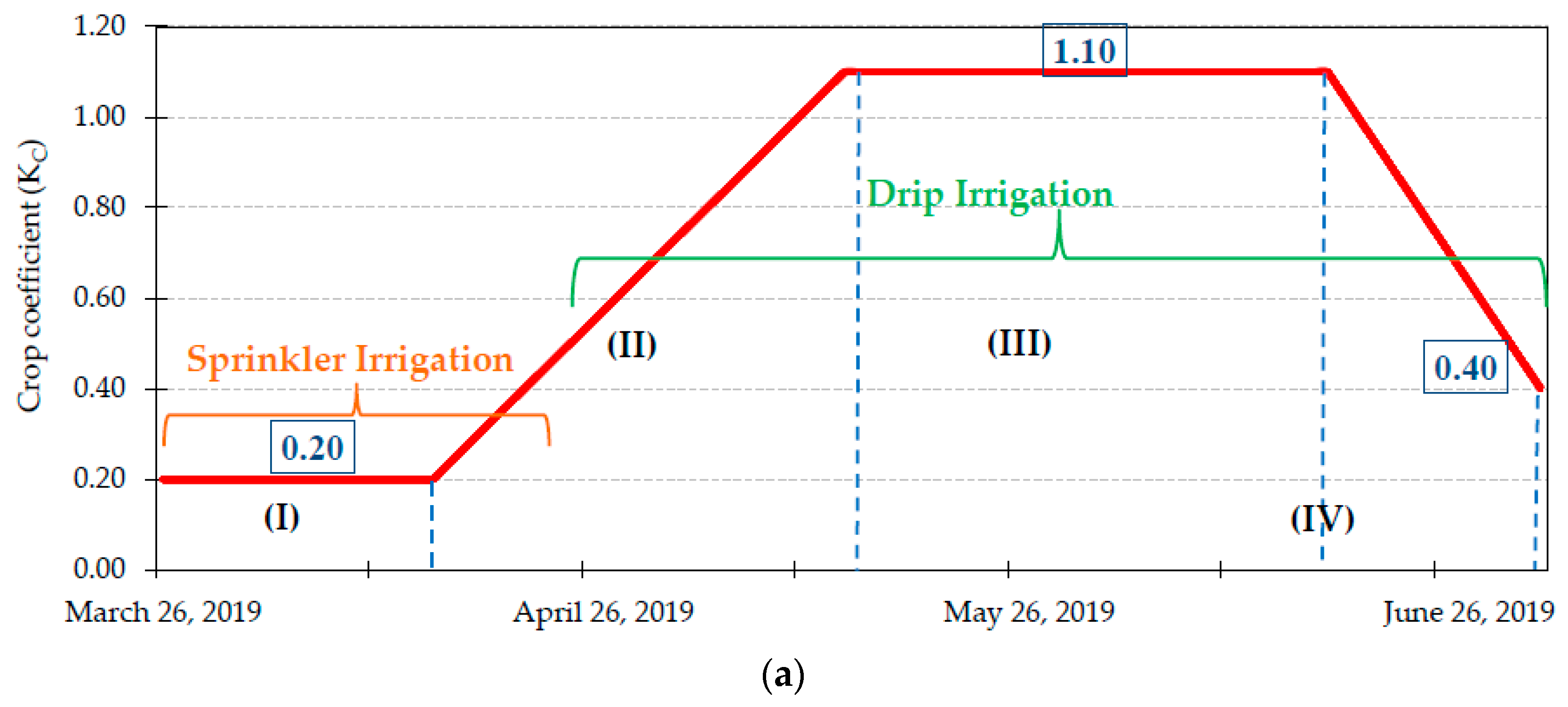
The crop coefficients used in the study were 0.2, 1.1, and 0.4 for the initial, mid-season, and late-season stages, respectively, based on prior reports [28] (Figure 3a). The corresponding daily ET_c values in mm were estimated over time and are shown in Figure 3b.

Table 2. Description of crop development across the different growth stages.

(I) Initial Stage			(II) Vegetative Growth	(III) Mid-Season Stage		(IV) Late-Season
KC = 0.2			KC1–KC2	KC2 = 1.1		KC2–KC3
20 days (20%)			29 days (30%)	34 days (35%)		15 days (15%)
Days:	1–8	12–29	32–52	56–68	72–84	84–98
Description:	Planting and Germination	Leaf and Plant Development	Bud Growth	Flowering and Pollination	Seed Development	Harvest

describes the progression of crop development across the different growth stages.

2.3. Planting, Irrigation Scheduling, and Fertigation Management

The 0.45 ha plot area (73.5 × 61.5 m) was planted with melons and Sudan grass in fall 2017 and spring to summer 2018, respectively, prior to 26 March 2019 planting of the grey stripe mammoth sunflower seed variety (supplied by Mountain Valley Seed Co., Salt Lake City, UT, USA). As described previously [23], the research field was planted on 81 rows, 73.5 m in length at 75 cm spacing (with a density of 300 plants per row), and a hand-moved sprinkler irrigation system was used for germination and stand establishment. A total of 350 kg·ha⁻¹ of monoammonium phosphate (MAP) 11-52-00 was applied as a pre-plant fertilizer before planting. A previously installed subsurface drip irrigation (SDI) system was utilized to irrigate the field for the remainder of the growing season with the first irrigation on 25 April. A supplemental nitrogen fertilizer application of 103 kg·ha⁻¹ of urea ammonium nitrate (UAN-32) (33 kg·ha⁻¹ N) was applied on 16 May (4th event of drip irrigation). The specifications of the sprinkler system and drip tape are presented in

Table 3. Sprinkler irrigation and drip tape system specifications.

(Sprinkler Irrigation)
Type	Radius	Application Rate:		Nozzle Size	Eleven irrigation events applied from 27 March to 19 April
Nelson R2000WF rotator	10 m	2.54 mm/h at 2.758 bar		10DK Blue = 2 mm
(Drip Tape)
Type	Wall Thickness	Diameter	Spacing	Flow Rate at 0.5516 bar (8 psi)	Nine irrigation events applied from 25 April to 1 July
Rivulis (506-12-450)	0.15 mm	1.50 cm	30.48 cm	0.001 m3/h

. Four different irrigation treatments were implemented: 100% ET_C (A, full irrigation), 95% ET_C (B), 80% ET_C (C), and 65% ET_C (D, deficit irrigation). On 7 June, 65% ET_C was achieved and the SDI irrigation system was not used in the western (deficit) section of the field after that date. Figure 4a,b shows the locations of various treatments (treatments A, B, and C consisted of nine drip lines for each treatment replicated three times while treatment D was in the western section of the field). The irrigation schedule and irrigation events and the total applied water for the sprinkler and SDI systems are presented in

Table 4. ET_C calculations and irrigation scheduling during the growing season.

System		Event Number	Date	Applied (mm)	Applied (m3)	Time (h)	Applied Cumulative (mm)	Required Cumulative (mm)
Sprinkler		1st	27 March	61	275.2	24.0	61	2
		2nd	30 March	14	63.1	5.5	75	6
		3rd	1 April	9	40.1	3.5	84	8
		4th	2 April	9	40.1	3.5	93	10
		5th	5 April	14	63.1	5.5	107	13
		6th	8 April	9	40.1	3.5	116	17
		7th	10 April	9	40.1	3.5	124	20
		8th	11 April	14	63.1	5.5	138	21
		9th	15 April	9	40.1	3.5	147	27
		10th	18 April	14	63.1	5.5	161	33
		11th	19 April	14	63.1	5.5	175	36
System	Note	Event Number	Date	Applied (mm)	Applied (m3)	Time (h)	Applied Cumulative (mm)	Required Cumulative (mm)
Drip	For the whole field (A–D)	1st	25 April	60	271.0	16.5	235	57
		2nd	10 May	23	103.0	13.0	258	145
		3rd	11 May	9	40.9	2.5	267	152
		4th	16 May	97	353.3	21.5	345	193
		5th	7 June	11	49.0	6.0	356	382
	A, B, C	6th	20 June	74	167.4	16.5	430	497
		7th	25 June	10	21.9	2.5	440	528
	A, B	8th	26 June	117	155.3	15.5	542	533
	A	9th	28 June	10	7.9	3.0	553	542 + 11 * = 553

* 11 mm added for the three days after the last irrigation till harvesting on 1 July.

.

2.4. Data Collection and Statistical Analysis

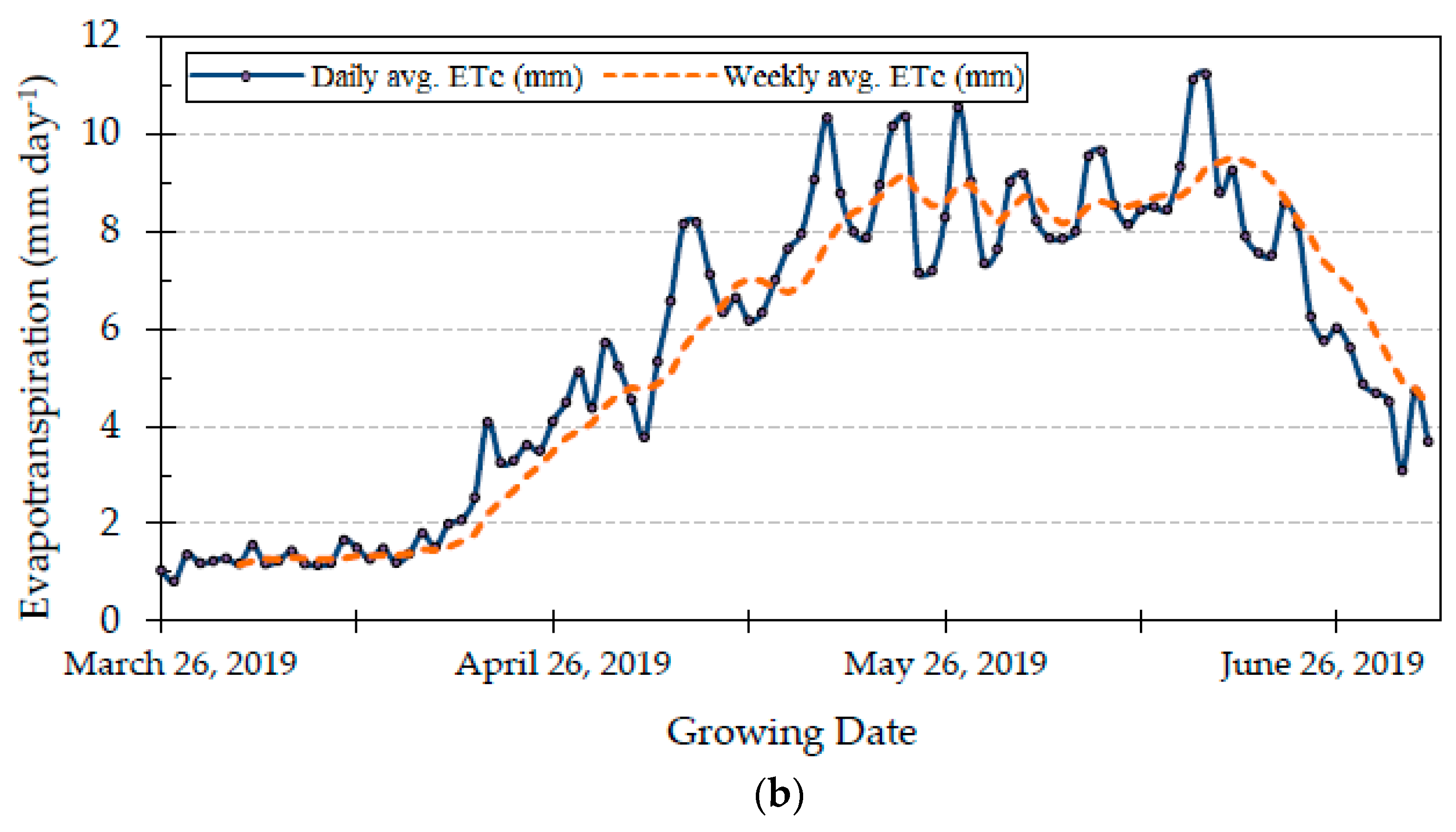
The irrigation source was located at the eastern side of the field, and the drip lines were aligned from east to west. Five observation wells, 3.8 cm in diameter and 3 m deep, were installed to determine groundwater depth and obtain water samples for analyses of salinity, chloride (Cl⁻), and other chemicals. Water table elevations were obtained, and water samples were collected manually weekly but we also used HOBO U20L-01 water level sensors [29] and HOBO U24-001 conductivity loggers [30] (Figure 4a) for continuous hourly measurements. The operation range for a U20L-01 sensor is from 0 to 9 m of water depth with very high accuracy (1.0 cm of water as a typical error). The sensor is individually calibrated while raw data is collected at multiple pressures and temperatures over the calibrated range of the logger [31]. The U24-001 conductivity sensor has a range of 0 to 10 dS·m⁻¹ with 3% error. We used weekly measurements as calibration points with linear compensation of temperature at 2.1%/°C for NaCl using the conductivity assistant feature in HOBOware software. Soil samples were collected within the top 120 cm (one sample for every 30 cm depth increment) at the same locations of the five observation wells for soil texture and chemical analysis prior to planting (to determine the requirements of the pre-plant fertilizer) and during the growing season for salinity and chloride measurements. Soil analyses were performed by Ward Laboratories, Inc. (Kearney, NE, USA) for the 40 soil samples in total (five well locations × four soil depths × two dates during the experiment).

Table 5. List of irrigation treatments and description.

Parameter	Value	Treatment	Description
Total Growth (Days) Total ETO (mm)	98 735	(A) 100% ETC (Control)	Regular drip irrigation applied for the whole season
Total ETC (mm)	553	(B) 95% ETC	526 mm, reached on 26 June at the eight drip event
Avg. KC	0.75	(C) 80% ETC	442 mm, reached on 25 June at the seven drip event
		(D) 65% ETC (Deficit)	360 mm, reached on 7 June at the five drip event

lists the irrigation treatments and the allocation of each treatment zone (6.8 m wide, nine rows for each treatment) is shown in Figure 4b. Soil matric potentials were recorded hourly using Irrometer (Riverside, CA, USA) Watermarks for the four different irrigation treatment zones at four soil depths within the active root zone: 30, 60, 90, and 120 cm (Figure 4b).

The relative yield and yield components (including the number of heads, weight of heads, number of seeds, and weight of seeds) were subjected to analysis of variance using the mixed procedure of SPSS Statistics 17 (IBM Corporation, New York, NY, USA). The effects of the full irrigation treatment (A) and the two reduced irrigations (B and C) were compared against the deficit irrigation treatment (D) to determine which yield components were impacted by deficit irrigation using a significance level (α) of 0.05. A separate analysis was conducted to determine the relative importance of different yield components on the relative yield and the Pearson’s coefficients of correlation (r) between relative yield and individual components were determined. One-way Analysis of variance, ANOVA test was performed between the different irrigation treatments for the seed yield to check if the p-value between treatments was significant or not. If the p-value was significant then a post test for multiple comparisons using Tukey HSD test was used.

2.5. Groundwater Contribution to Crop Evapotranspiration and Seed Yields

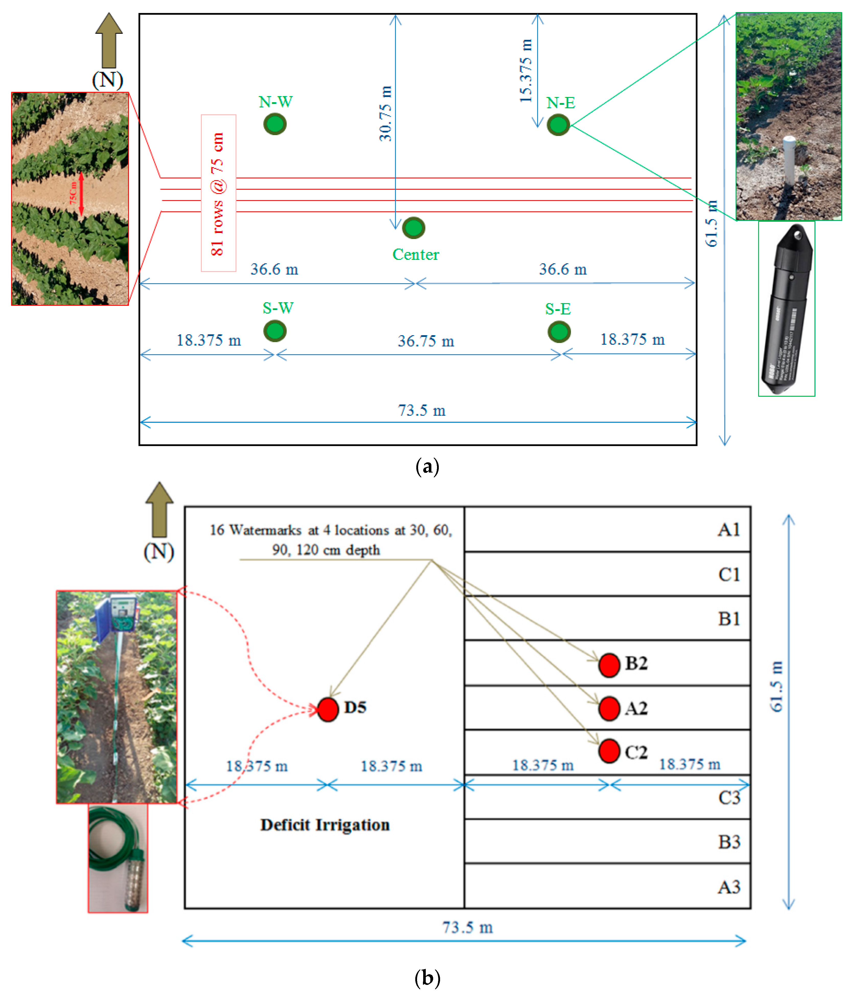
In general, salinity from shallow groundwater or in the soil profile near the active root zone has the potential to negatively impact root water uptake and could adversely impact yield and actual evapotranspiration [32]. An estimate of the pre-planted soil salinity along the root depth of the crop of interest is thus essential to determine the likely impact of existing salinity on plant performance, and the results of such an analysis might influence the decision to plant a different, more resistant crop. In order to investigate the water table contribution (WTC) to crop evapotranspiration, the chloride mass balance method [21] was used to estimate water table contribution to ET_C (under the assumption that the crop will not extract chloride) and then compare the IWUE related to seed yields. Eighteen harvest locations of 3.5 m² each (two sunflower rows × 4.6 m strip) were selected at the center of the two sections of the field, nine locations at the eastern side of the field (3 × 3) representing the A, B, and C treatments multiplied by the three replicates and nine locations at the deficit side (Figure 5a). Twenty soil samples (at four depths, 30 cm each × five locations) were collected on 9 April 2019 and again on 28 June 2019, and the corresponding chloride concentrations and electrical conductivities of groundwater (EC_GW) and soil salinities were recorded. After applying the chloride mass balance for the 1.20 m soil depth at the five locations of the observation wells, the groundwater contribution and the added salinity from groundwater were calculated.

The inverse distance weight method (IDW) [33] in ArcGIS was utilized to spatially interpolate the distribution of the EC_GW and groundwater depths across the field to generate corresponding values for the 18 harvest locations. The relationship between yield and ET_C, applied irrigation water, or transpiration is known as the crop production function [7]. Among several models that were developed to define these relationships, Stewart’s equation [22] is the most frequently used model to define the relationship between yield and ET_C or applied water. This function describes the yield response factor (k_y) when applied for the total growth stage [27].

(1 − Y/Y_max) = k_y (1 − ET/ET_max)

(1)

where Y is the yield under water deficit, Y_max is the maximum yield under full irrigation, and ET and ET_max are the evapotranspiration under deficit irrigation and full irrigation. Values of k_y indicate the sensitivity of sunflower to deficit irrigation. Additionally, the best-fit relation (highest R² value) between yield and applied irrigation water was obtained for the whole growing season for the four irrigation treatments. IWUE was determined to evaluate the productivity of applied irrigation water in the treatments at the level of crop yield production (IWUE = yield/applied irrigation water, where seed yield is in kg·ha⁻¹, applied irrigation water is in m³·ha⁻¹, and IWUE is in kg·m⁻³) [34]. After harvesting the 18 locations on 1 July, the sunflower stalks were shredded (Figure 5b) and the drip tape was removed. The observation wells were then flagged and the field was chiseled and leveled.

3. Results

3.1. Plant Development Stages

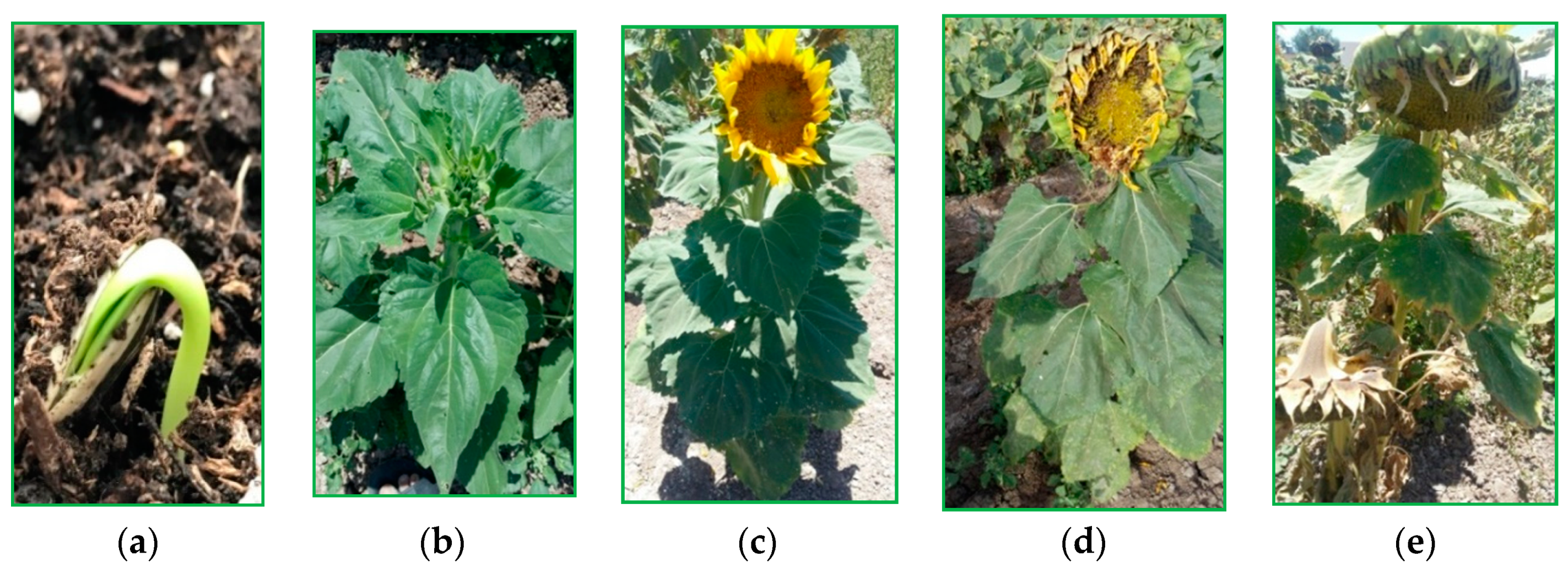
The field was planted on 26 March 2019 when the average daily temperature for the initial stage for germination was 21.5 °C (range = 6–23 °C). The seeds germinated after ca. six days (1 April with 147 °C GDD). The average daily temperature during the vegetative growth stage (between the initial stage and the mid-growth stage) was 24.3 °C (range = 20–25 °C), and maximum canopy cover of ca. 90% was reached in mid-May (ca. 50 days after planting) and flowering commenced on 22 May. The irrigation treatments of 95%, 80%, and 65% were based on the total evapotranspiration (ET_C) of the fully irrigated crop, and the deficit irrigation treatment of 65% was reached on 7 June (between the initiation of flowering and pollination during the mid-growth stage). All treatments received the same amount of irrigation water until flowering. Therefore, water stress could not have affected the timing of floral initiation. Similarly, the additional 33 kg·ha⁻¹ of N (16.5, 8.25, 8.25 kg·ha⁻¹ in the form of urea, ammonium, and nitrate, respectively) was applied to the entire field on 16 May before reaching the 65% ET_C deficit treatment. Therefore, the temperature would have been the primary factor affecting the vegetative period from starting leaf development on 7 April to just before the heads became visible on 12 May (Figure 6a–e shows images and corresponding dates for the various growth stages during the 98-day growing season). Based on the calculations of the growing degree days (GDD) [35], the plants transitioned to flowering after 1107 °C GDD (at least one open disc floret on ≥50% of plants), reached physiological maturity (PM) on 15 June after 1982 °C GDD, and completed grain filling after an additional 478 °C GDD, for a total of 2460 °C GDD (for completion of dry-down and direct harvesting); these values are similar to prior results [1,36].

3.2. Water Table Contribution and Salinity Measurements

The depth to groundwater was recorded manually weekly from the beginning of the experiment and then hourly from 16 April (the date of installation of the HOBO water level sensors) until harvest on 1 July from the five observation wells (Figure 7). The depth to groundwater on 16 April (the first record of the water table by HOBO U20L-01 sensors) varied for the five sampling locations. This may be attributed to the variance of hydraulic conductivity in the horizontal direction because of the heterogeneity of soil in this specific area (area No. 44) of the research center. As such, variable recharge of the groundwater likely occurred while applying the pre-irrigation event on 20 March for herbicide application before planting on 26 March. In general, depth to groundwater fluctuated from 1.25 to 2.25 m during the drip irrigation events. The shallow groundwater table was recharged from the irrigation water only after the first and fourth drip irrigation events, but only in the western section of the field. For the first drip irrigation (25 April), the depth to water table decreased from 2.0 to 1.5 m for the south-west well, and from 2.0 to 1.8 m after the fourth drip irrigation event (16 May). The impact of the long first drip irrigation event on groundwater depth was also apparent for the north-west well where the depth to water table decreased by ca. 20 cm (from 1.6 to 1.4 m). There was no apparent groundwater recharge from the irrigation water in the eastern section of the field. An overall increase in depth to groundwater was observed in the N-W and S-W sections of the field as compared to the N-E and S-E sections (Figure 7) due to the cessation of irrigation in the deficit (western) portion of the field. A decrease in depth to groundwater of ≤7.4 cm was recorded after the sixth irrigation event (when only the A, B, and C treatments were irrigated), and a reduction of ≤11.7 cm was recorded after the eighth irrigation event (when only the A and B treatments were irrigated). The application of deficit irrigation (i.e., withholding of additional irrigation) in the western portion of the field from 7 June to 1 July resulted in a noticeable increase in groundwater depth and indicated a likely groundwater contribution to sunflower ET (Figure 7).

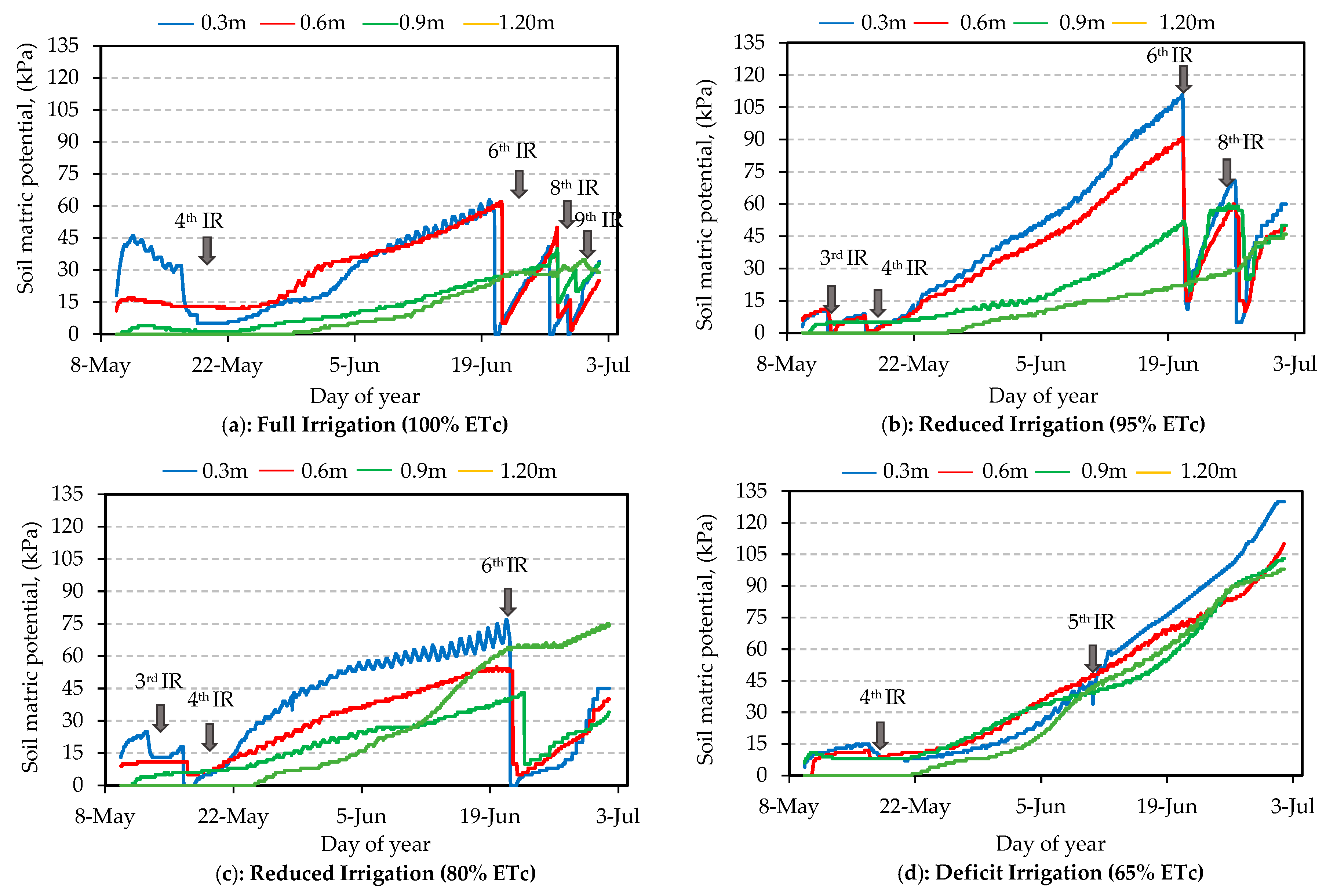
Soil matric potentials were measured in centibars (kPa) by watermarks sensors for the 120-cm root depth. Three data loggers were located in the eastern section for the A, B, and C treatments (each data logger had four Watermark sensors) and one additional data logger was located in the center of the western section (treatment D; 65% ET_C) (Figure 4b). Variation in soil matric potential throughout the duration of the experiment for the four locations representing the different irrigation treatments is shown in Figure 8. Overall, the soil matric potential was the lowest (higher soil moisture content) for the full irrigation (treatment A; 100% ET_C) (Figure 8a) while the highest values (lower soil moisture content) were recorded for deficit irrigation (treatment D; 65% ET_C) (Figure 8d) with values of 62 and 126 kPa for the Watermarks at 30 cm depth in treatments A and D, respectively. A sudden drop in the soil matric potential levels was observed four times at the shallowest depth (30 cm), and three times at the 0.60 and 0.90 m depths for the full irrigation treatment (Figure 8a). These drops in matric potential were due to the application of irrigation water through the fourth, sixth, eighth, and ninth drip events which are indicated in Figure 8a with brown arrows. For the 95% ET_C (irrigation treatment B), four sudden drops in matric potential for the top 60 cm of the soil were obtained, and only two drops in matric potential at 90 cm depth were observed after the six and the eight drip events (Figure 8b). Although treatments A and B received the same amount of water until the eight drip event on 26 June, a large difference in matric potential was observed for the sensors at 30 cm (62 and 109 kPa, for A and B treatments) and 60 cm (60 and 90 kPa, for A and B treatments). A large difference in matric potential was also observed for the two shallowest sensors in the 80% ET_C and 100% ET_C treatments (75 and 53 kPa for sensors at 30 and 60 cm) (Figure 8c). This difference in matric potential is mainly due to the location of sensor in relation to the drip line. This is the case of the sensors probes at shallow depths (30, 60 cm) as the other two sensors (at lower depths) had very similar readings across treatments A, B, and C during the period in which they received the same amount of irrigation water. Soil matric potential within the deficit treatments increased rapidly after 25 May (Figure 8d).

In addition to measuring applied irrigation water, the contribution of the shallow saline groundwater table to sunflower evapotranspiration was estimated. The chloride mass-balance method described by Wallender et al. [37] and performed by Bali et al. [21] for alfalfa in the Imperial Valley was employed for the period between 9 April and 28 June. In addition to the determination of chloride levels in irrigation water and groundwater (Table S1 in supplementary file), the chloride concentrations for each 30 cm depth increment of the soil profile in the root zone (120 cm) at each of the five locations were determined. The salinity in dS·m⁻¹ along the 120 cm soil depth near the five observation wells is presented in Table S2 in the supplementary file. WTC was estimated by averaging the values of the contribution at the three locations in the deficit portion of the field (N-W, center, and S-W). The difference in chloride concentrations from initial application of the deficit until the end of the experiment was calculated for each soil layer. The contribution of irrigation water was considered assuming that 40%, 30%, 20%, and 10% of irrigation water was distributed along the four soil layers. Thus, the contribution from groundwater (in kg) was obtained for each layer and converted to a depth of groundwater (in m) based on the chloride concentrations for groundwater for each well.

Table 6. Water table contribution (WTC) to sunflower water use for each soil layer (cm) for the deficit irrigation (65% ET_C) treatment where salinity for the applied irrigation water, EC_a = 1.13 dS·m⁻¹ and chloride Cl⁻ = 98 mg·L⁻¹.

Treatment	Depth (cm)	Avg. Increment Cl− (mg/L)	Added Chloride Cl− (kg/m)	WTC cm and %
Deficit 65% ETC	0–30	249 ± 101	0.0748	9.03 cm = 16.3% of the ETC of the fully irrigated crop
	30–60	199 ± 60	0.0610
	60–90	19 ± 4	0.0057
	90–120	83 ± 21	0.0249

summarizes the water table contribution to sunflower crop water use since the last irrigation for the deficit treatment. The average added chloride mass (kg·m⁻³) for the four 30-cm depth increments along with the 1.20 m soil depth between 7 June and 1 July for the deficit portion of the field is also summarized in Table 6.

The deficit treatment (D; 65% ET_C) included three wells (N-W, S-W, and center). The average groundwater contribution from those three locations was 9.03 cm, which corresponds to 16.31% of the ET_C of the fully irrigated crop. This compensation from groundwater to the 35% shortage of applied water was calculated for the deficit period from 7 June until harvest on 1 July. This groundwater contribution was relatively small since the deficit irrigation started during the late stage of growth.

Table 7. Average soil matric potential (ψ_s) within the 120 cm soil depth (average daily values) (kPa) on 28 June, toward the end of the growing season.

Depth	ψs (kPa)	ψs (kPa)	ψs (kPa)
	Treatment (B)	Treatment (C)	Deficit
0–30 cm	45.8	22.6	114.9
30–60 cm	36.4	23.2	93.3
60–90 cm	40.3	25.1	95.4
90–120 cm	41.8	69.0	93.6

summarizes the reading of the daily soil matric potential in kPa within the 120 cm soil depth on 28 June.

3.3. Crop Yield, Production Functions, and Water Use Efficiency

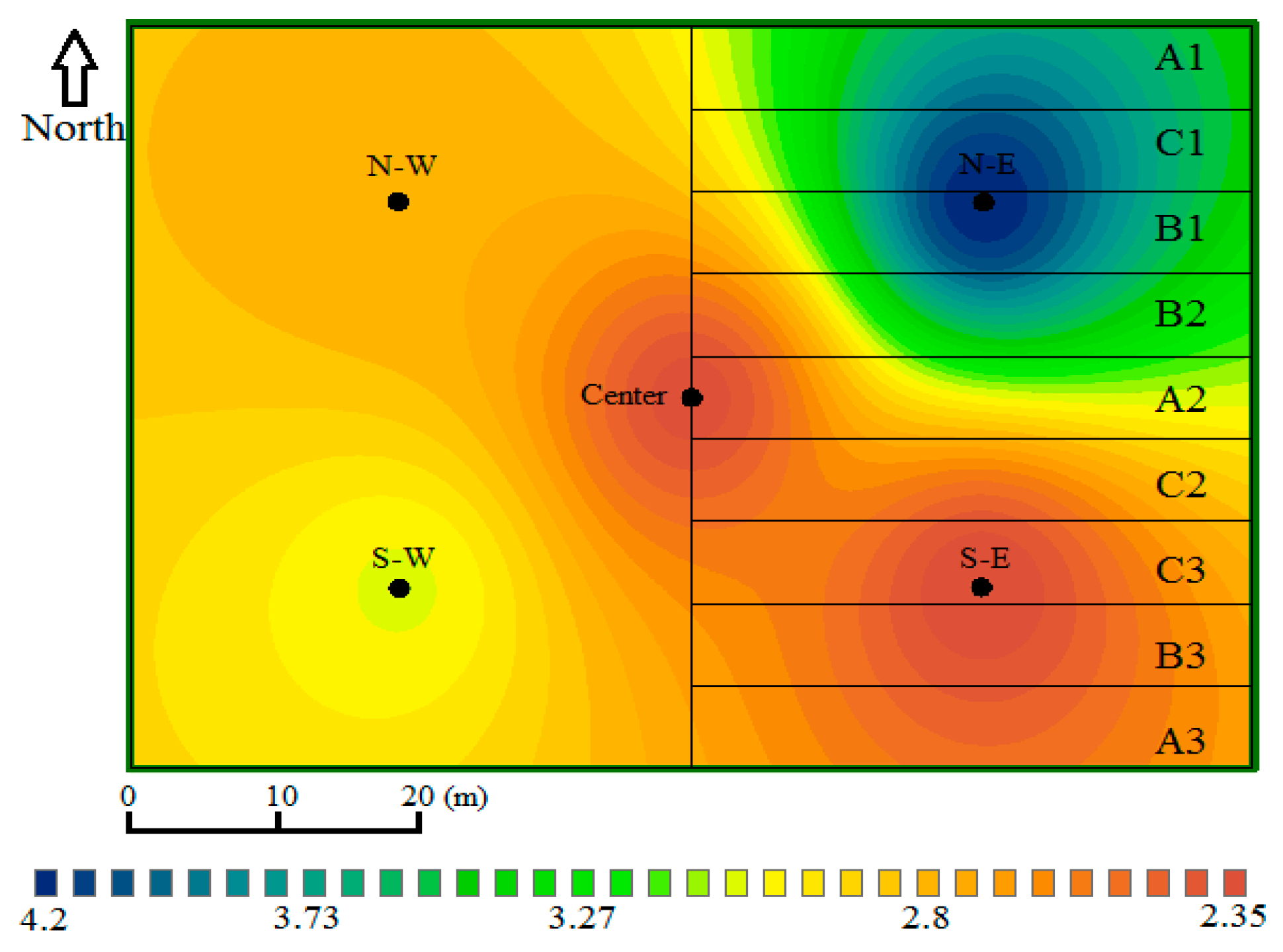
Seed yield for sunflower was obtained from the 18 harvest locations where the number and weight of heads and the number and weight of seeds were counted and measured. While the WTC and salinity were only calculated at the five selected locations, the IDW interpolation was used to obtain the salinity for the 18 harvest locations (Figure 9). Thereafter, the average soil profile salinity for each irrigation treatment was obtained to compare the yield of the different irrigation treatments to determine if soil salinity had an impact on yield. Most of the salinity levels in the soil profile were within the salinity threshold level for sunflower, and therefore, any reduction in yield was mainly related to water stress and not salinity (

Table 8. Electrical conductivities at the locations of the Watermarks from inverse distance weight method (IDW) interpolation for the four soil depths in 9 April; the salinity of the applied irrigation water (EC_a) was 1.13 dS·m⁻¹.

Period	Soil Sample Depth (cm)	EC (dS·m−1)
		(A2)	(B2)	(C2)	(D5)
From 9 April to 28 June	0–30	2.40	2.49	2.36	2.47
	30–60	2.72	3.05	2.41	2.33
	60–90	3.61	4.43	2.71	2.83
	90–120	3.80	4.95	2.80	3.45
Avg. salinity	0–120	3.13 ± 0.68	3.73 ± 1.15	2.57 ± 0.22	2.77 ± 0.50

). It summarizes the salinity levels at the watermarks sensors locations (A2, B2, C2, and D5) within the 1.20 m soil depth from the IDW interpolation of the analyzed samples from the observation wells. The maximum obtained yield was 2048.9 kg·ha⁻¹ for 100% ET_C where salinity ranged from 2.49 to 3.88 dS·m⁻¹ among the three replicated zones (A1, A2, and A3). The yields of the other three treatments (B, C, and D) were 1879.9, 1688.1, and 1710.3 kg·ha⁻¹, respectively. The corresponding relative yields were calculated and estimated to be 91.8%, 82.4%, and 83.5% for B, C, and D (

Table 9. Yield components and irrigation water use efficiency (IWUE) calculations for the 18 harvest locations.

Treatment	Section	Soil Salinity * (dS·m−1)	No. of Heads	Wt. of Heads (g)	No. of Seeds	Wt. of Seeds (g)	Seed Yield (kg·ha−1)	Relative Yield (%)	Applied Irrigation (IR) (m3·ha−1)	IWUE (kg·ha−1·mm−1)
A	1	3.88	83	959	12,759	704	2011	100	5537	3.63
	2	3.08	101	1038	14,307	728	2079			3.76
	3	2.49	128	1251	13,440	720	2056			3.71
Avg.			104	1083	13,502	717	2049 ± 34.59			3.70
B	1	4.16	92	968	11,789	631	1802	86.64		3.43
	2	3.73	115	1138	12,356	660	1887	90.74	5260	3.59
	3	3.38	125	1271	12,773	683	1951	93.83		3.71
Avg.			111	1126	12,306	658	1880 ± 74.75	91.75		3.57
C	1	4.11	88	802	9865	579	1653	79.51	4430	3.73
	2	2.59	92	920	10,097	592	1693	81.40		3.82
	3	2.36	147	1290	10,248	601	1718	82.63		3.88
Avg.			109	1004	10,070	591	1688 ± 32.79	82.39		3.81
D	1	2.83	115	1095	11,010	590	1686	81.09	3599	4.69
	2	2.81	111	1130	11,897	593	1695	81.49		4.71
	3	2.81	140	1184	11,968	604	1725	82.95		4.79
	4	2.83	148	1264	10,330	619	1767	85.00		4.91
	5	2.89	80	947	10,894	597	1705	81.99		4.74
	6	3.01	94	953	9412	600	1714	82.43		4.76
	7	3.1	94	983	8765	608	1738	83.59		4.83
	8	3.09	93	972	8692	598	1708	82.14		4.75
	9	3.03	140	1237	9365	579	1655	79.57		4.60
Avg.			113	1085	10,259	599	1710 ± 31.88	83.48		4.75

Note: * soil salinity (dS·m⁻¹) is from the average records between 9 April and 28 June of the four soil layers (0–120 cm) including the added salinity from groundwater.

).

The yield components (number of heads, weight of heads, number of seeds per head, and weight of seeds per head) were examined to investigate the effect of the application of the deficit irrigation with 65% ET_C with comparison to the effects of the other three treatments; full irrigation and the two reduced irrigation treatments.

Table 10. Significance of the impact of full/reduced irrigation (A, B, and C) vs. deficit irrigation (D) on yield components of sunflower.

Irrigation Treatment	No. of Heads	Wt. of Heads	No. of Seeds	Wt. of Seeds
(A, B, C)–(D)	p = 0.664	p = 0.845	p = 0.009 *	p = 0.009 *
	F = 0.19675	F = 0.03926	F = 8.60512	F = 8.60512

Note: * significant at p < 0.05.

shows that seed weight and the number of seeds produced were both significantly reduced under deficit irrigation, whereas the other yield components were unaffected. The correlation analysis provided a positive association between the relative yield and seed weight, and number of seeds while a very slightly negative (−0.033) non-significant correlation was observed with the number of heads (

Table 11. Pearson’s correlation coefficients (r) between yield/yield components of sunflower.

Yield Components	Relative Yield	No. of Heads	Wt. of Heads	No. of Seeds	Wt. of Seeds
Relative yield	1	−0.033	0.192	0.811 ****	0.996 ****
Number of heads		1	0.924 ****	0.091	−0.009
Weight of heads			1	0.278	0.216
Number of seeds				1	0.824 ****
Weight of seeds					1

Note: **** significant at p ≤ 0.0001 level.

). For the 18 collected sampling locations for harvesting, relative yield and seed weight were found to be strongly correlated, (R = 0.996, n = 18, p = 0.00001). The relative yield and the number of seeds were found to be strongly positively correlated, R = 0.811, n = 18, p = 0.00004. However, head weight had no detectable relationship with relative yield (r = 0.192, p = 0.446); similarly, there was no significant correlation between the number of heads and relative yield (r = −0.033, p = 0.895).

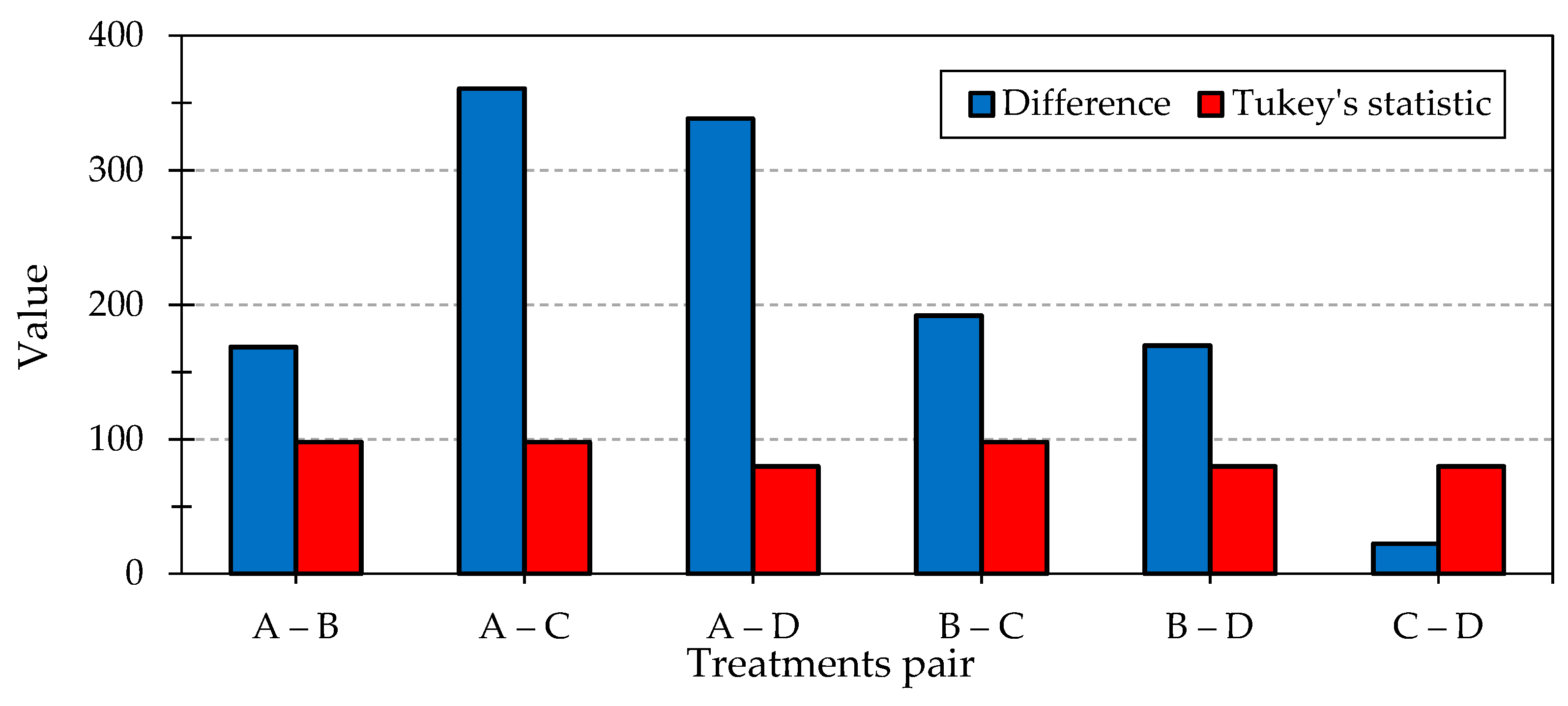
The ANOVA test result showed a significant difference of mean seed yields between the four irrigation treatments while the p value equals 2.69 × 10⁻⁸ and F = 61.322. Tukey HSD test showed that the means of the following pair of treatments are significantly different; 100% ETc—95% ETc and 100% ETc—80% ETc and 100% ETc—65% ETc and 95% ETc—80% ETc and 95% ETc—65% ETc.

Table 12. ANOVA and Tukey test results.

ANOVA
Source of variation	Degrees of freedom, df	Sum of square, SS	Mean square, MS	F statistic	p-Value
Between treatments	3	313,328.95	104,442.98	61.322	2.6922 × 10−8
Error (within treatments)	14	23,844.67	1703.19
Total	17	337,173.62
Tukey Analysis for the Differences in Seed Yields
Treatments Pair	Difference		Standard error, SE	Tukey’s statistic, Tα *	p-Value
A–B	168.67		23.827	97.941	0.000978
A–C	360.67		23.827	97.941	2.17 × 10−7
A–D	338.33		19.455	79.969	3.74 × 10−8
B–C	192.00		23.827	97.941	0.000285
B–D	169.67		19.455	79.969	0.000128
C–D	22.33		19.455	79.969	0.847914

* Tukey’s statistic, T_α = q_α·(p, f)$\sqrt{\frac{MS \mathrm{error}}{r}}$ where p is the number of treatments, f is the number of degrees of freedom associated with the mean square error (MS error), and r is the number of replicates.

summarizes the one way ANOVA test and the Tukey test results while Figure 10 shows the difference to critical means for the six pairs of treatments that have significant p-values.

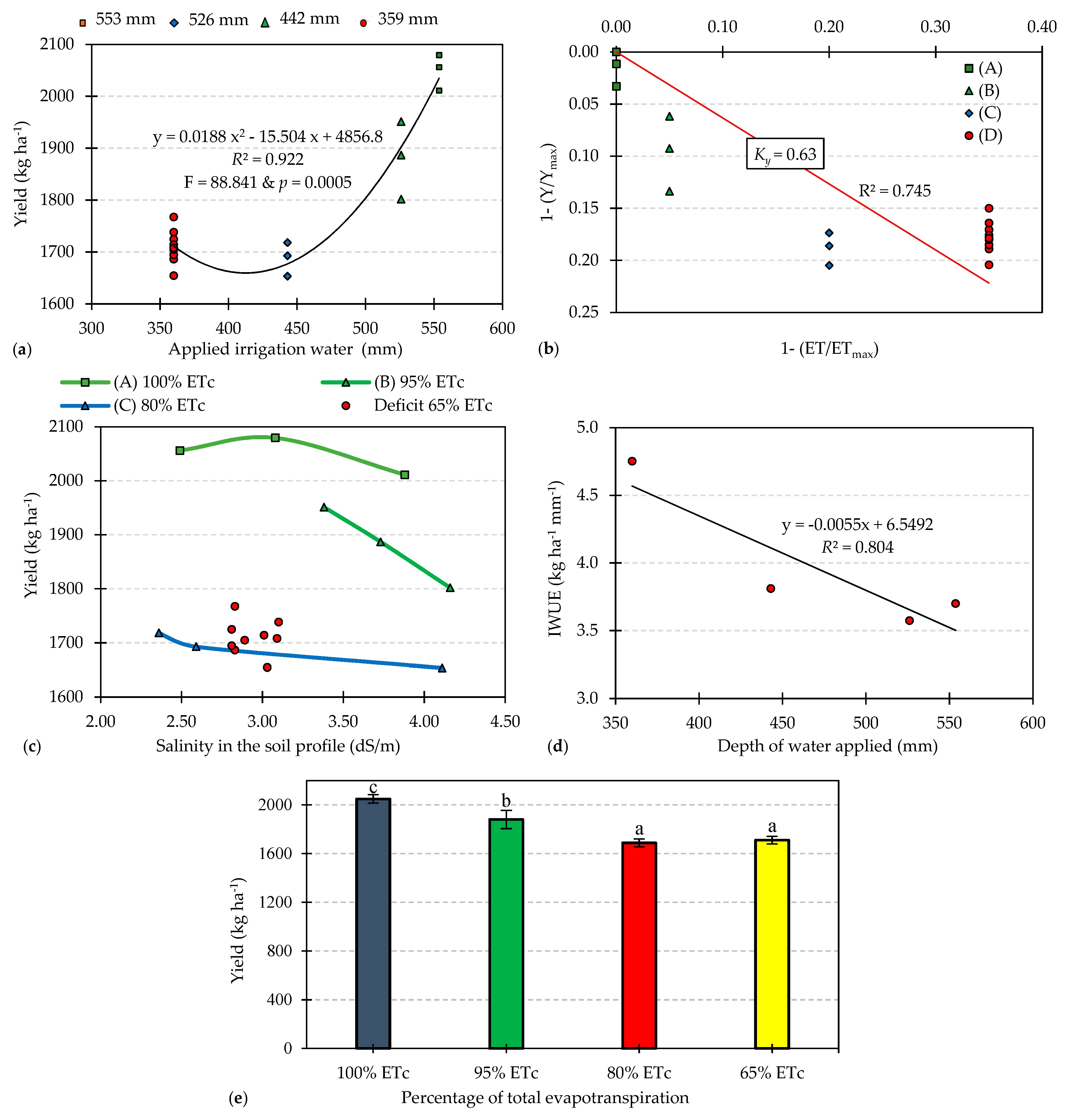
The water production function was determined by plotting the observed yield (kg·ha⁻¹) for each irrigation treatment on the y-axis, and the corresponding applied irrigation water, IR, in mm on the x-axis (Figure 11a). The 2nd order polynomial relation, yield = 0.0188 × (IW)² − 15.504 × IW + 4856.8, was obtained between applied irrigation water and seed yield. The standard deviation and standard errors were 140.9 and 33.2 kg·ha⁻¹, respectively, and the coefficient of determination of this relationship was R² = 0.922, p = 0.0005. The yield response factor, k_y, across the growing season was determined for all treatments from the equation that relates proportional IW decreases to proportional yield decreases (Figure 11b) via linear regression, adjusted through the origin. The slope of the line, k_y, was 0.63 across the full growing season. The overall reduction in sunflower yield was less than proportional to the decrease in water use (ET_C, crop evapotranspiration) (k_y was <1), likely due to the groundwater contribution under water deficit. This coincides with previous results showing that sunflower is relatively insensitive to water deficit [2], but k_y changes among the different growth stages for early-stage (0.50), bud growth (1.00), flowering (0.80), and seed production (0.25), respectively.

To determine the effect of the added salinity from the groundwater on the soil profile within the first 120 cm of soil depth, the relationship between salinity (dS·m⁻¹) and yield (kg·ha⁻¹) was investigated for each irrigation treatment (Figure 11c). For the widest range of salinity among the four irrigation treatments for each three zones of A, B, and C and the nine zones of D, we estimated only a 3.8% reduction in yield for treatment C (from 1718.29 to 1653.43 kg·ha⁻¹) due to the increase in salinity from 2.36 to 4.11 dS·m⁻¹. The irrigation water use efficiencies for A, B, C, and D were 3.70, 3.57, 3.81, and 4.75 kg·ha⁻¹·mm⁻¹, respectively. The highest IWUE obtained was for the deficit treatment where the 65% ET_C was achieved on 7 June when more than 50% of plants had open florets. This indicated that the 35% deficit that was applied during the late stage of growth likely occurred during a period when the plants had access to groundwater from the shallow aquifer. It appears that the average water use efficiencies for the four treatments decreased with increasing irrigation, which is consistent with the view that sunflower is capable of tolerating water stress (Figure 11d). The relationships between the percentage of ET_C of applied irrigation water and yield are shown in Figure 11e.

4. Discussion

Across all treatments, the average depth to groundwater was only reduced appreciably after the initial application of SDI (Figure 7). During the SDI, the soil moisture sensors (Figure 8) revealed a similar pattern of wetting/drying between irrigation events in the top 25% and 50% of the soil profile (i.e., 30 and 60 cm), but this pattern differed deeper in the soil profile (i.e., at 90 and 120 cm) where the soil matric potential increased more slowly. This result indicates that most of the water uptake was from the top 50% of the soil profile. This is also supported by the increase in Cl⁻ mass during the deficit irrigation period in treatment D, where most of the increase in Cl⁻ concentration and water uptake occurred in the top 50% of the soil profile. The presumably high root water uptake from the top 60 cm of soil depth, in addition to evaporation from the top 30 cm (particularly during the early stages of growing period when crop cover was <30%) produced a much higher rate of increase in soil matric potential in this portion of the soil profile.

During the vegetative growth period, plants across the field exhibited similar growth responses. The minimum recorded fractions of the total available water (TAW) during this time were 0.85 and 0.92 at the 60 and 90 cm depth increments, respectively, based on the soil matric potential measurements from the deficit treatment on 7 June (Figure 8d). These results agree with earlier findings showing that transpiration after anthesis, when the leaves are fully expanded, is dependent upon stomatal behavior that is not impacted until TAW fractions below 0.85 are reached [9,38]. The considerable variation in the vertical distribution of salinity throughout the soil profile (i.e., the top 120 cm; Table 7) between the start of SDI and harvest was likely due to the added salts in the western section of the field through the WTC from the saline groundwater.

The observed variation in relative yield among the different irrigation treatments was directly related to the seed weight, and the number of seeds produced rather than head weight. Similarly, the number of heads produced did not significantly impact relative yield across treatments (Table 11). The observed variation in seed yield (kg·ha⁻¹) was dependent on the size and number of seeds was in general agreement with the results of Joshi et al. [39], who found that yield is correlated with 1000-seed weight. At the same time, Fereres et al. [40] found that decreases in harvest index in sunflower due to water deficits were mostly due to adjustments in seed number as opposed to seed weight. The lack of an effect of head traits on relative yield makes sense in that the deficit irrigation was not applied until late in the growing season after head had been produced and flowering had commenced. The corresponding numbers and weights of the seeds produced between 100% ET_C and 65% ET_C treatments were 24% and 16.5%, respectively. This greater decrease in seed number than in seed weight suggests that, under deficit irrigation, seed weight compensates for the reduction in overall seed production, which is similar to the results obtained by Langeroodi et al. [41].

The coefficient of determination for the relationship between yield (kg·ha⁻¹) and applied irrigation water (mm) was 0.92. Notably, there was only one extremely minor precipitation event during the entire 98-day growing season (0.6 mm on 16 April). This strong correlation between the irrigation and yield can likely be attributed to the continued application of irrigation water late in the season. The IWUE for A, B, and C treatments are very similar (3.7, 3.6, 3.8 kg·ha⁻¹·mm⁻¹), and the differences in the applied water were in the final week of growth (Table 9). However, the occurrence of a late-season deficit appears to have resulted in an increase in water use efficiency, similar to the results shown by Demir et al. [7]. Researchers have, however, found that there is no significant decrease in IWUE when irrigation water is increased beyond the full irrigation needs [42]. Furthermore, IWUE values obtained from this study are within the range of variation obtained by others [38,43].

The reduction in relative yield of 16.5% for the deficit treatment (65% ET_C) is similar to the reduction observed in treatment C (80% ET_C), likely due to the groundwater contribution compensating for the water shortage in the late growth stage after full root development. Although the added salinity from groundwater was the highest for deficit treatment, with an increase in soil salinity of 1.86 dS·m⁻¹, this additional salinity did not appear to have impacted the yield of this treatment negatively. Indeed, the maximum obtained recorded salinity was 4.11 dS·m⁻¹, which is considerably less than the threshold salinity of sunflower (4.80 dS·m⁻¹) [10].

5. Conclusions

In this study, we evaluated the contribution of shallow saline groundwater to sunflower crop water use under deficit irrigation. The average groundwater contribution for the deficit treatment (65% ET_C) was 9.03 cm which represented 16.3% of the total applied irrigation water in the fully irrigated treatment. The maximum and minimum seed yields were 2048 and 1710 kg·ha⁻¹ for the 100% ET_C and 65% ET_C treatments, respectively. The minimum relative yield obtained for 65% ET_C was 83.5% (i.e., 16.5% reduction). The crop response factor, k_y, was 0.63 and the irrigation water use efficiencies were 4.75 and 3.70 kg·ha⁻¹·mm⁻¹ for the deficit and full irrigation treatments, respectively. The maximum salinity value in the active root zone was 4.11 dS·m⁻¹ (in the 80% ET_C treatment) and had no apparent effect on yield. Taken together, these results suggest that irrigation deficits in sunflower are likely to be at least partially offset by contributions from available groundwater as well as possible increases in crop water use efficiency, thereby minimizing yield reductions. As such, deficit irrigation of sunflowers in a semi-arid region could be used as a tool to conserve water and/or address water shortages.

References

- Long, R.; Gulya, T.; Light, S.; Bali, K.; Mathesius, K.; Meyer, R. Sunflower Hybrid Seed Production in California. 2019. Available online: https://anrcatalog.ucanr.edu/Details.aspx?itemNo=8638 (accessed on 1 July 2019).
- Steduto, P.; Hsiao, T.C.; Fereres, E.; Raes, D. Crop Yield Response to Water; FAO Irrigation and Drainage Paper 66; FAO: Rome, Italy, 2012; p. 500. Available online: http://www.fao.org/docrep/016/i2800e/i2800e00.htm (accessed on 1 September 2019).
- Miller, J. Hybrid Selection and Production Practices. In Sunflower Production; Duane, R.B., Ed.; Extension Publication A-1331; North Dakota State University (NDSU): Fargo, ND, USA, 2007; p. 117. Available online: https://www.ag.ndsu.edu/pubs/plantsci/rowcrops/a1331-04.pdf (accessed on 1 September 2019).
- Seiler, G.J.; Gulya, T.J. Sunflower: Overview. In Encyclopedia of Food Grains, 2nd ed.; Academic Press: Oxford, UK, 2016; pp. 247–253. [Google Scholar] [CrossRef]
- Radanović, A.; Miladinović, D.; Cvejić, S.; Jocković, M.; Jocić, S. Sunflower genetics from ancestors to modern hybrids–A review. Genes 2018, 9, 528. [Google Scholar] [CrossRef] [PubMed] [Green Version]
- Chen, M.; Kang, Y.H.; Wan, S.Q.; Liu, S.P. Drip irrigation with saline water for oleic sunflower (Helianthus annuus L.). Agric. Water Manag. 2009, 96, 1766–1772. [Google Scholar] [CrossRef]
- Demir, A.O.; Goksoy, A.T.; Buyukcangaz, H.; Turan, Z.M.; Koksal, E.S. Deficit irrigation of sunflower (Helianthus annuus L.) in a sub-humid climate. Irrig. Sci. 2006, 24, 279–289. [Google Scholar] [CrossRef]
- Verma, S.B.; Shrivastava, A.K.; Jha, J.K. Irrigation Resources; Scientific Publishers: Jodhpur, India, 2016; ISBN 9789386237415. [Google Scholar]
- Sadras, V.O.; Villalobos, F.J.; Fereres, E. Leaf expansion of field-grown sunflower in response to water status. Agron. J. 1993, 85, 560–570. [Google Scholar] [CrossRef]
- Francois, L.E. Salinity effects on four sunflower hybrids. Agron. J. 1996, 88, 215–219. [Google Scholar] [CrossRef] [Green Version]
- Katerji, N.; Van Hoorn, J.W.; Hamdy, A.; Mastrorilli, M. Salt tolerance classification of crops according to soil salinity and to water stress day index. Agric. Water Manag. 2000, 43, 99–109. [Google Scholar] [CrossRef]
- Zeng, W.; Xu, C.; Huang, J.; Wu, J.; Ma, T. Emergence rate, yield, and nitrogen-use efficiency of sunflowers (Helianthus annuus) vary with soil salinity and amount of nitrogen applied. Commun. Soil Sci. Plant Anal. 2015, 46, 1006–1023. [Google Scholar] [CrossRef]
- Zhu, J.; Zeng, W.; Ma, T.; Lei, G.; Zha, Y.; Fang, Y.; Wu, J.; Huang, J. Testing and Improving the WOFOST Model for Sunflower Simulation on Saline Soils of Inner Mongolia, China. Agronomy 2018, 9, 172. [Google Scholar] [CrossRef] [Green Version]
- Zeng, W.; Xu, C.; Wu, J.; Huang, J. Sunflower seed yield estimation under the interaction of soil salinity and nitrogen application. Field Crop. Res. 2016, 198, 1–15. [Google Scholar] [CrossRef]
- Shahbaz, M.; Ashraf, M.; Akram, N.A.; Hanif, A.; Hameed, S.; Joham, S.; Rehman, R. Salt-induced modulation in growth, photosynthetic capacity, proline content and ion accumulation in sunflower (Helianthus annuus L.). Acta Physiol. Plant. 2011, 33, 1113–1122. [Google Scholar] [CrossRef]
- Li, C.; Zhang, Z. Effects of Ionic Components of Saline Water on Irrigated Sunflower Physiology. Water 2019, 11, 183. [Google Scholar] [CrossRef] [Green Version]
- Schultz, E.; DeSutter, T.; Sharma, L.; Endres, G.; Ashley, R.; Bu, H.; Markell, S.; Kraklau, A.; Franzen, D. Response of sunflower to nitrogen and phosphorus in North Dakota. Agron. J. 2018, 110, 685–695. [Google Scholar] [CrossRef] [Green Version]
- Sadras, V.O.; Hall, A.J.; Trapani, N.; Vilella, F. Dynamics of rooting and root-length: Leaf-area relationships as affected by plant population in sunflower crops. Field Crop. Res. 1989, 22, 45–57. [Google Scholar] [CrossRef]
- Moutonnet, P. Yield Response Factors of Field Crops to Deficit Irrigation. In Deficit Irrigation Practices; Water Rep. 22; FAO: Rome, Italy, 2002; pp. 11–16. [Google Scholar]
- Nasim, W.; Ahmad, A.; Bano, A.; Olatinwo, R.; Usman, M.; Khaliq, T.; Wajid, A.; Hammad, H.M.; Mubeen, M.; Hussain, M. Effect of nitrogen on yield and oil quality of sunflower (Helianthus annuus L.) hybrids under sub-humid conditions of Pakistan. Am. J. Plant Sci. 2012, 3, 243–251. [Google Scholar] [CrossRef] [Green Version]
- Bali, K.M.; Grismer, M.E.; Snyder, R.L. Alfalfa water use pinpointed in saline, shallow water tables of Imperial Valley. Calif. Agric. 2001, 55, 38–43. [Google Scholar] [CrossRef]
- Stewart, J.I.; Hagan, R.M.; Pruitt, W.O. Water Production Functions and Predicted Irrigation Programs for Principal Crops as Required for Water Resources Planning and Increased Water Use Efficiency; Report 14-06-D-7329; U.S. Department of Interior, Bureau of Reclamation, Engineering and Research Center: Denver, CO, USA, 1976; p. 80.
- Eltarabily, M.G.; Burke, J.M.; Bali, K.M. Effect of deficit irrigation on nitrogen uptake of sunflower in the low desert region of California. Water 2019, 11, 2340. [Google Scholar] [CrossRef] [Green Version]
- Available online: https://casoilresource.lawr.ucdavis.edu/gmap/ (accessed on 1 July 2019).
- Available online: https://websoilsurvey.nrcs.usda.gov/app/WebSoilSurvey.aspx (accessed on 1 July 2019).
- Available online: https://cimis.water.ca.gov/Stations.aspx (accessed on 1 July 2019).
- Doorenbos, J.; Kassam, A.H. Yield response to water. In FAO Irrigation and Drainage; Paper 33; FAO: Rome, Italy, 1979; p. 193. [Google Scholar]
- Snyder, R.L.; Orang, M.; Bali, K.; Eching, S. Basic Irrigation Scheduling Program (BISe); University of California Land, Air, and Water Resources Biomet Website: Oakland, CA, USA, 2014; Available online: http://biomet.ucdavis.edu/irrigation_scheduling/bis/BIS.htm (accessed on 1 April 2019).
- Available online: https://www.onsetcomp.com/products/data-loggers/u20l-01 (accessed on 1 September 2019).
- Available online: https://www.onsetcomp.com/products/data-loggers/u24-001 (accessed on 1 September 2019).
- Available online: https://www.onsetcomp.com/files/manual_pdfs/17153-G%20U20L%20Manual.pdf (accessed on 1 September 2019).
- Nilahyane, A.; Islam, M.A.; Mesbah, A.O.; Garcia y Garcia, A. Effect of Irrigation and Nitrogen Fertilization Strategies on Silage Corn Grown in Semi-Arid Conditions. Agronomy 2018, 8, 208. [Google Scholar] [CrossRef] [Green Version]
- Setianto, A.; Triandini, T. Comparison of Kriging and Inverse Distance Weighted (IDW) Interpolation Methods in Lineament Extraction and Analysis. J. Southeast Asian Appl. Geol. 2013, 5, 21–29. [Google Scholar] [CrossRef]
- Ayers, R.S.; Westcot, D.W. Water Quality for Agriculture. In FAO Irrigation and Drainage; Paper 29 (Rev. 1); FAO: Rome, Italy, 1985. [Google Scholar]
- Available online: http://ipm.ucanr.edu/calludt.cgi/WXSTATIONDATA?MAP=imperial.html&STN=ELCENTRO.A (accessed on 1 April 2019).
- Miller, P.; Lanier, W.; Brandt, S. Using Growing Degree Days to Predict Plant Stages; MT200103 AG 7/2001; Ag/Extension Communications Coordinator, Communications Services, Montana State University-Bozeman: Bozeman, MO, USA, 2001. [Google Scholar]
- Wallender, W.W.; Grimes, D.W.; Henderson, D.W.; Stromberg, L.K. Estimating the Contribution of a Perched Water Table to the Seasonal Evapotranspiration of Cotton. Agron. J. 1979, 71, 1056–1060. [Google Scholar] [CrossRef]
- Sadras, V.O.; Villalobos, F.J.; Fereres, E.; Wolfe, D.W. Leaf response to soil water deficits: Comparative sensitivity of leaf expansion rate and leaf conductance in field-grown sunflower (Helianthus annuus L.). Plant Soil 1993, 153, 189–194. [Google Scholar] [CrossRef]
- Joshi, V.R.; Heitholt, J.J.; Garcia, Y.; Garcia, A. Response of confection sunflower (Helianthus annuus L.) grown in a semi-arid environment to planting date and early termination of irrigation. J. Agron. Crop Sci. 2017, 203, 301–308. [Google Scholar] [CrossRef]
- Fereres, E.; Gimenez, C.; Fernandez, J.M. Genetic variability in sunflower cultivars under drought. I. Yield relationships. Aust. J. Agric. Res. 1986, 37, 578–582. [Google Scholar] [CrossRef]
- Langeroodi, A.R.S.; Kamkar, B.; da Silva, J.A.T.; Ataei, M. Response of sunflower cultivars to deficit irrigation. Helia 2014, 37, 37–58. [Google Scholar] [CrossRef]
- Goksoy, A.T.; Demir, A.O.; Turan, Z.M.; Dagustu, N. Responses of sunflower (Helianthus annuus L.) to full and limited irrigation at different growth stages. Field Crop. Res. 2004, 87, 167–178. [Google Scholar] [CrossRef]
- Karam, F.; Lahoud, R.; Masaad, R.; Kabalan, R.; Breidi, J.; Chalita, C.; Rouphael, Y. Evapotranspiration, seed yield and water use efficiency of drip-irrigated sunflower under full and deficit irrigation conditions. Agric. Water Manag. 2007, 90, 213–223. [Google Scholar] [CrossRef]
Figure 1.
The location map of (a) the UC Desert Research Center (DREC) and (b) the experimental field within DREC.
Figure 2.
(a) Daily (reference evapotranspiration—ETo) (mm) and (b) daily average temperature (°C) during the growing season.
Figure 3.
(a) Crop coefficients for the different growing stages. (b) Estimated daily (solid blue) and weekly (orange dashed line) evapotranspiration (ETC) (mm) during the growing season.
Figure 4.
(a) Field dimensions and locations of observation wells (green circles). (b) The layout of irrigation treatments showing deficit irrigation in the western section and the replicates of the full and reduced irrigation treatments (A, B, and C) in the eastern section (nine zones total, nine rows each).
Figure 5.
(a) Illustration of the 18 harvest sections (nine from the eastern section + nine from the western deficit section) with a length 4.6 m and taken from the two middle rows for each zone; specific row numbers are indicated. (b) Shredding of the stalks of one of the field sections following harvest.
Figure 6.
Development stages of plant growth for the full irrigation (treatment A) 100% ETC (Control). (a) Seedling emergence on 2 April. (b) Bud growth on 8 May when plant height ranged from 40 to 50 cm. (c) Initiation of flowering on 7 June, when plant height ranged from 100 to 130 cm. (d) Post-flowering on 20 June. (e) Approaching physiological maturity on 26 June, prior to harvest.
Figure 7.
Depth to groundwater (m) for the five observation wells from 16 April to 1 July.
Figure 8.
Soil matric potential for the hourly measurements from the four Watermark sensors within the 120 cm soil depth (soil water tension starts to increase above 0 kPa as the soil starts to dry below saturation) for (a) zone A2, (b) zone B2, (c) zone C2, and (d) zone D5, irrigation events (IR) indicated by arrows.
Figure 9.
Inverse distance weighted interpolation of salinity (dS·m−1) from the five locations within the 1.20 m soil profile including the added salinity from groundwater.
Figure 10.
The comparison between the absolute difference between the means and the Tukey’s statistic for the six significant pairs of treatments.
Figure 11.
(a) Relationship between yield (kg·ha−1) and applied irrigation water and the production function. (b) Relationship between yield and evapotranspiration, along with the response factor. (c) Relationship between the added salinity in the soil profile (dS·m−1) and yield (kg·ha−1) for the four irrigation treatments. (d) Relationship between water use efficiencies and the applied depth of water (mm). (e) Yield as a function of the percentage of ETC applied; error bars denote means ± SD of the replicates. Bars with different letter denote significance in treatments at p < 0.05; analyzed by Tukey post-hoc test.