A Decision Support System for Irrigation Management: Analysis and Implementation of Different Learning Techniques

Abstract

Automatic irrigation scheduling systems are highly demanded in the agricultural sector due to their ability to both save water and manage deficit irrigation strategies. Elaborating a functional and efficient automatic irrigation system is a very complex task due to the high number of factors that the technician considers when managing irrigation in an optimal way. Automatic learning systems propose an alternative to traditional irrigation management by means of the automatic elaboration of predictions based on the learning of an agronomist (DSS). The aim of this paper is the study of several learning techniques in order to determine the goodness and error relative to expert decision. Nine orchards were tested during 2018 using linear regression (LR), random forest regression (RFR), and support vector regression (SVR) methods as engines of the irrigation decision support system (IDSS) proposed. The results obtained by the learning methods in three of these orchards have been compared with the decisions made by the agronomist over an entire year. The prediction model errors determined the best fitting regression model. The results obtained lead to the conclusion that these methods are valid engines to develop automatic irrigation scheduling systems.

1. Introduction

Water is a limiting factor in agricultural production. This fact is intensified in regions where water is scarce. In these regions, the importance of properly managing irrigation is a fundamental factor for sustainable production. There are agricultural techniques that have made it possible to optimize irrigation management, from the use of drip irrigation systems to regulated deficit irrigation strategies able to maintain yields with lower irrigation volumes [1,2].

Information and communication technologies (ICT) have contributed to the sustainable management of water in agriculture. The deployment of wireless sensor networks in crops using Internet of Things (IoT) technologies and the remote management of data with cloud computing have allowed massive monitoring of agricultural variables, which generate a large amount of information [3,4]. This information helps the agronomist to determine the water status of the soil–plant–atmosphere continuum and to make decisions about irrigation, and whether different deficit irrigation strategies adapted to phenology and physiology of the crop should be implemented [5]. In addition, the democratization of IoT technologies for monitoring soil and weather variables is allowing a wide diffusion of water saving tools in home contexts [6,7].

However, the continuous modernization of irrigation systems needs to implement equipment that allows an automated scheduling of irrigation. It must include sensors to provide different parameters [8,9]. Traditionally, these parameters are related to environmental conditions and provide information about the full crop water requirements using weather stations [6] as well as the soil’s water status or volumetric content, which indicate the water availability for the plant. The most commonly used soil parameter sensors are those that use dielectric properties, since they are cheap and flexible [10,11], although its correct operation requires complex calibration, taking into account factors such as soil texture and structure, temperature, and water salinity [12,13,14] besides the spatial variability of the soil conditions [15]. Other sensors such as thermal and multispectral cameras, satellites, or infrared radiometers (IR) are used to estimate water crop needs [16,17,18,19].

Regarding irrigation automation, soil sensors have started to be used for this purpose, considering water matric potential [20] and volumetric water content [21], with thermal sensors [22] and, recently, their combination with wireless technologies for flexible implementation [9]. These systems use fixed or dynamic thresholds of the soil, and measure atmospheric or plant parameters for irrigation actuation [23,24].

However, irrigation management can take into account more variables, including the hydro-physical properties of certain soils, the parameters related to other crops, their stages of development, water quality [25,26], and factors related to productivity, fruit quality, and the implementation of deficit irrigation strategies [27], which prevent the proper functioning of irrigation thresholds.

Systems based on machine learning (ML) techniques use the previous irrigation management experience of a human expert to train a system to reproduce that expert behavior. Fuzzy logic, artificial neural networks (ANNs), or regression procedures have been used recently for automatic irrigation management [28,29,30].

Decision support systems (DSSs) are ML applications that use the knowledge of an agronomist (human expert) to learn irrigation scheduling patterns and emulate human activities in decision-making. Additionally, DSSs permit a continuous learning process (while being used) and adapt their performance to context changes or different objectives [31]. Therefore, DSSs in agriculture are useful tools for optimal irrigation management and have demonstrated good behavior [32]. These systems have been defined and implemented over several years in the agricultural sector for a large range of applications, not only for developing irrigation management [33] but also crop growth models [34], and financial and agricultural management models [35]. In some applications for irrigation management, knowledge-based learning models have been developed using climate data provided by weather station networks [36].

Different algorithms are used for water needs estimations in automatic irrigation systems based on ML. ANN [37,38] and support vector regression (SVR) [33] algorithms are widely used for DSS development. In [39], k-nearest neighbor (kNN) and adaptive boosting (AdaBoost) algorithms were compared with an ANN for the estimation of potato water needs. The authors in [40] compared SVR with multivariate adaptive regression splines (MARS) and M5 model tree (M5Tree) in modeling reference evapotranspiration (ETo). Genetic algorithms (GAs) [41] and random forest regression (RFR) [42] have also been used for water needs estimation.

This paper presents the development of an irrigation decision support system (IDSS) for irrigation management optimization in citrus trees. The system uses the following information obtained automatically by in-the-field sensors: (1) weather data, (2) the amount of applied water data from the previous week, and (3) soil water status and water quality data. We also considered aspects such as meteorological predictions, the type of crop, and the phenological stage on which the model performs the irrigation calculation. The system was trained using reports made by agronomists for determining the irrigation frequency and doses on a weekly basis. Three regression learning algorithms were compared for performance purposes: linear regression (LR), SVR, and RFR. The models were evaluated using leave-one-out cross-validation (LOOCV) and random 90-10 shuffle cross-validation techniques.

The irrigation amount estimated for an entire year by the IDSS was compared with the irrigation water applied by the agronomists, allowing us to compare the performance of different learning algorithms.

Section 2 describes the material and methods used for the development of the IDSS. Section 3 summarizes the results obtained and a discussion. The conclusions are described in Section 4.

2. Materials and Methods

Figure 1 shows the process used by an agronomist (expert) to determine the amount of irrigation.

ETo (reference evapotranspiration) is obtained from meteorological variables and represents the effect of the weather on net crop water requirements, while Kc (crop coefficient) indicates the specific characteristics of the crop and its effect on water needs (the type of crop, the development and phenological stage, etc.). In a third stage, the quality of the irrigation water, the uniformity coefficient of the irrigation system, the field size, etc., allow for determining the real volumes of irrigation. This value gives an approximate idea of the amount of water needed to satisfy full crop water requirements. This value is modulated with the water status of the soil to obtain the volume of irrigation to contribute to the crop.

The main goal of the IDSS is to calculate the irrigation doses that have to be applied to the crop. This decision is taken automatically based on the information provided by the sensors and the prediction of a machine learning system. The aim of this component, therefore, is to mimic a human expert (agronomist) in the decision-making process.

The IDSS described in this paper was trained using different varieties of citrus trees (orange, mandarin, and lemon trees) and cultivated in different plots. For each one of them, weekly irrigation reports (carried out by the agronomist) were used to train the system.

In the following paragraphs, the main parts used to develop the IDSS are described: (i) the integrated information platform that provides the soil and irrigation data, (ii) the crops and plots where the data and irrigation reports were obtained and where the IDSS was tested, and (iii) the architecture of the different machine learning algorithms implemented in the IDSS.

2.1. Data Collection Platform

The information about the soil and weather conditions is provided by wireless devices called nodes, developed by Widhoc Smart Solutions (CEDIT, Fuente Álamo 30320, Spain). The wireless nodes collect and send data using Wi-Fi or GPRS links. A cloud server stores and indexes the data for further processing purposes. The nodes are powered by solar panels and rechargeable batteries.

The main variables collected by the nodes are as follows:

(1)

soil matric potential measured by MPS-6 sensors (Decagon devices, Inc., Pullman, WA 99163, USA) (Figure 2a);

(2)

volumetric water content (VWC, soil moisture) measured by 10HS sensors (Decagon devices, Inc. Pullman, WA, USA) (Figure 2b);

(3)

volumetric water content, bulk electrical conductivity, and soil temperature measured by 5TE sensors (Decagon Devices, Inc. Pullman, WA, USA) (Figure 2c);

(4)

volume of water supplied during the previous week, measured with flowmeters (Apator POWOGAZ JS-04, Poland) (Figure 2d).

Each node samples the variables every 15 min and sends the information to a data server. This server establishes communication with the nodes and the integration of the databases (the information from customers and equipment is stored securely). The processed information is shown on a website-customizable front-end layer.

Information about weather conditions is provided by the IMIDA (Instituto Murciano de Investigación y Desarrollo Agrario y Alimentario, 30150 Murcia, Spain). This public research institution has deployed a network with 49 climatic stations that cover the region of Murcia (SIAM) [43] (Figure 3).

The network is widely used to determine the ETo, in addition to other variables such as temperature (T), relative humidity (RH), global radiation (GR), wind speed (WS), rainfall (RF), dew point (DP), and vapor pressure deficit (VPD).

The weather information, belonging to the SIAM network, is automatically integrated into the cloud server to complement the soil and water data from the nodes.

2.2. Plot and Report Description

The data were collected from nine commercial orchards of citrus trees located in the Southeast Spain, specifically in the region of Murcia. This is a semiarid zone where the water is very scarce and drip irrigation is commonly used. The irrigation criteria followed was to maximize the yield per unit area.

Table 1. Crops and reports used in the training process.

Orchard	Crop Type	Variety	Age	Field Size	Sensors	Water EC	Report Number
1	Lemon	Fino 49	11 years	5.5 ha	1xMPS6 2x10HS	1.2 dSm−1	32
2	Lemon	Fino 95	10 years	6.0 ha	1xMPS6 2x10HS	2.2 dSm−1	31
3	Orange	Lanelate	8 years	6.0 ha	2xMPS6 1x10HS	1.6 dSm−1	44
4	Lemon	Fino 95	12 years	6.0 ha	2xMPS6 1x10HS	2.5 dSm−1	60
5	Mandarin	Clemenville	12 years	6.0 ha	2xMPS6 1x10HS	1.0 dSm−1	44
6	Mandarin	Orri (Malla)	8 years	5.5 ha	2xMPS6 1x10HS	2.0 dSm−1	70
7	Mandarin	Orri	7 years	5.5 ha	2xMPS6 1x10HS	2.0 dSm−1	69
8	Orange	Lane	8 years	6.0 ha	2xMPS6 1x10HS	2.0 dSm−1	60
9	Lemon	Verna	3 years	6.0 ha	2xMPS6 1x10HS	1.6 dSm−1	74

shows the main characteristics of the orchards and the numbers of reports used in the training process.

The weekly reports to train the system were generated by two different technicians. They used the information from the automatic weather stations closest to the orchard placement, including crop parameters and other data such as water quality and soil sensor information. They also needed the amount of water applied to the orchard during the previous week. The generated reports, as a final result, suggest the total amount of water for the following week. The total number of reports available is 484, for nine different citrus crops located in Southeast Spain.

2.3. Irrigation Decision Support System (IDSS)

The proposed IDSS is a trained system that automatically predicts the amount of irrigation water needed for the orchard. A supervised training process was used. Irrigation reports performed by the agronomist in the orchard were used as the ground-truth.

In order to cover the best options of automatic learning systems, regressive techniques were implemented. The regression methods that were used to predict the agricultural technician criteria are LR, RFR, and SVR. A detailed description of each method and their corresponding parameters selection are presented below.

Two validation techniques (LOOCV and 90-10 shuffle cross-validation) were used to test the goodness of every model, as suggested in [44].

The root-mean-square error (RMSE), given in Equation (1), was used to obtain the accuracy of the forecasting models:

$$RMSE = \sqrt{{\displaystyle \sum }_{t = 1}^n\frac{{(y_i-{\widehat{y}}_i)}^2}{n}}$$

(1)

where $n$ is the number of data, $y_i$ is the actual output of the instance i, and ${\widehat{y}}_i$ is the corresponding estimated output. It is a global and very standard error measure where lower values mean higher accuracy in the predictions. Note that the RMSE is measured on the same scale as the output variable, so a simple comparison among the RMSE of the forecasting methods is enough to evaluate their performance when the output variable is the same for all forecasting methods.

2.3.1. Description of the Output and Input Variables

In this research, the same output and input variables were used for the three forecasting methods (LR, RFR, and SVR). The output (response variable) in all cases was the total amount of irrigation water for the next week suggested by the agronomists (given in their reports).

• Regarding the set of possible input variables, the selection was made according to the main information used by the agronomists when developing the irrigation reports, such as the total water needs (TWN), the soil water status, the amount of water applied previously, and the critical period of the crop: in the case of citrus trees, the main critical periods are flowering and fruit setting (Stage I), and a second period when fruit is growing fast (Stage II).
• However, there are more factors that might affect irrigation prediction (such as the weather prediction, the possible irrigation cutoff in the area, etc.), and those factors are not taken into account by the agronomist. This could be a limitation of this IDSS.
• The selection of a suitable set of features is crucial for good performances in the prediction models. In this sense, a selection procedure similar to that depicted in [36] was developed. The inputs that perform best in this new context were the following:
• daily average of the matric potential of the last 5 d (five inputs);
• the TWN (one input);
• the water applied (sensor measured) during the previous week (one input);
• a binary value indicating whether or not the crop is in a period where the fruit is gaining weight (one input).
• The daily average of the soil matric potential gives representative information about the conditions of the soil in the previous week. The TWN provides the theoretical irrigation volume for the crops in a specific area with specific weather conditions. The quantity of water for the last week is a hint of what the water requirement for the next week should be, as the water requirements of one week and the next are highly correlated. Finally, the period of the crop helps to finer tune the irrigation quantity: periods without fruit are less critical than those in which the fruit is present on the crop [27,45].

Due to the nature of the output (the amount of water for the next week), we selected the regression methods described below to obtain the predictions.

2.3.2. Linear Regression

LR is a classical statistical method that explains a target variable $Y$ (called a response variable) as a linear function of a set of features $X_j$ controlled by the researcher (called regressors or predictors).

In general, the multiple LR model can be expressed as follows:

$$Y_i={\beta }_0+{\beta }_1{x}_{i,1}+\dots +{\beta }_k{x}_{i,k}+{ϵ}_i i=1,2,\dots n$$

(2)

where n denotes the sample size. The ${\beta }_j$ parameters of the model are estimated using the least squares criteria. In general, some of the proposed predictors by the researcher might be not significant (that is, irrelevant when the rest of the predictors are considered in the model), so it is important to provide simpler models when it is possible. There are different methods to achieve a simplified model, such as stepwise, forward, and backward selection methods. The results of the model selection depend on the data being analyzed. In the present research, the three selection methods were applied to the dataset before estimating the multiple LR model, and the same results were obtained.

The main advantage of the LR method against other ML methods is the fast computation time in which the parameters of the model are estimated. Under a suitable theoretical framework, it allows inferences on the regression parameters and predictions. Although the LR method has shown good behavior in many contexts and fields, its efficiency is limited to linear relationships between the response variable and the predictors. However, real problems might present nonlinear and complex relationships between them.

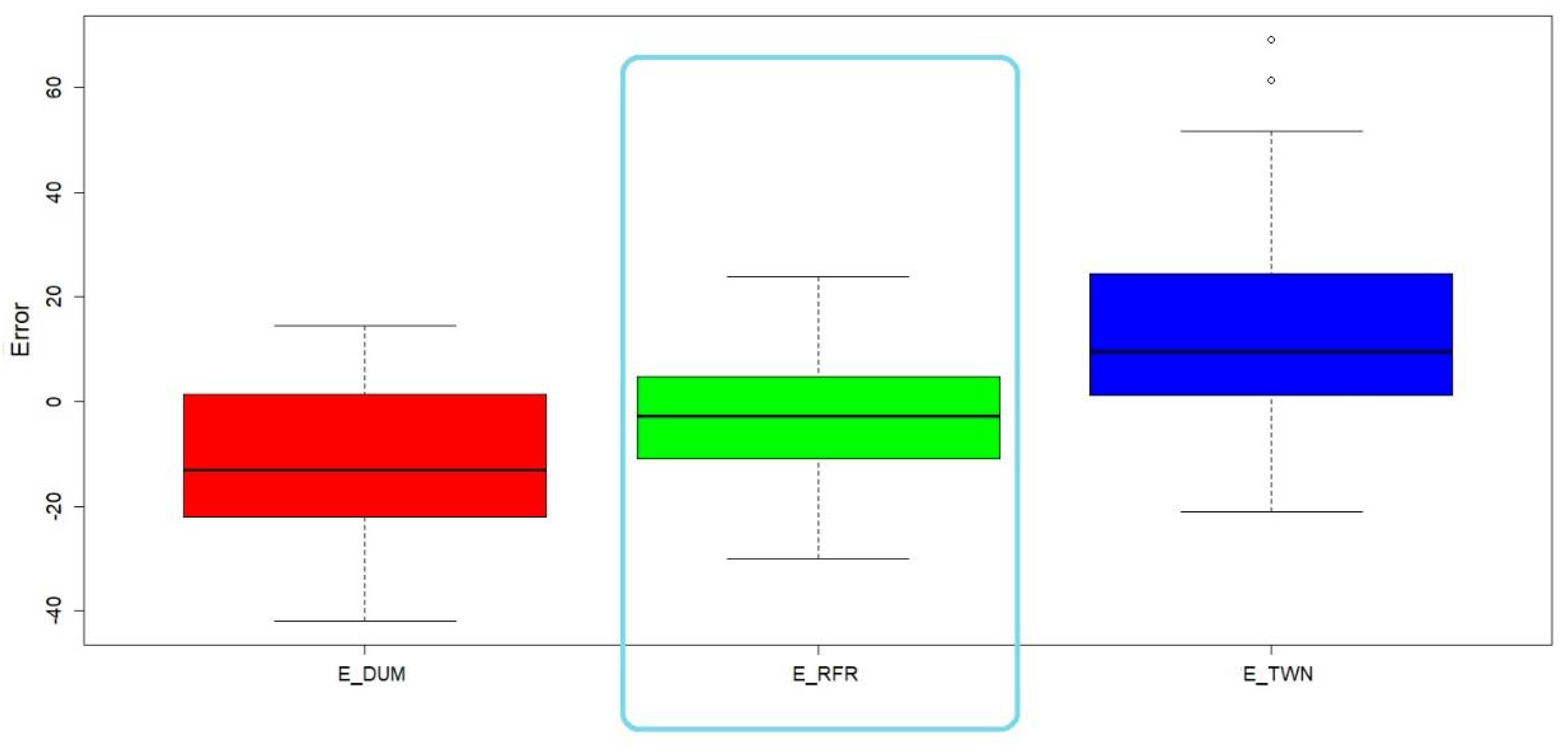
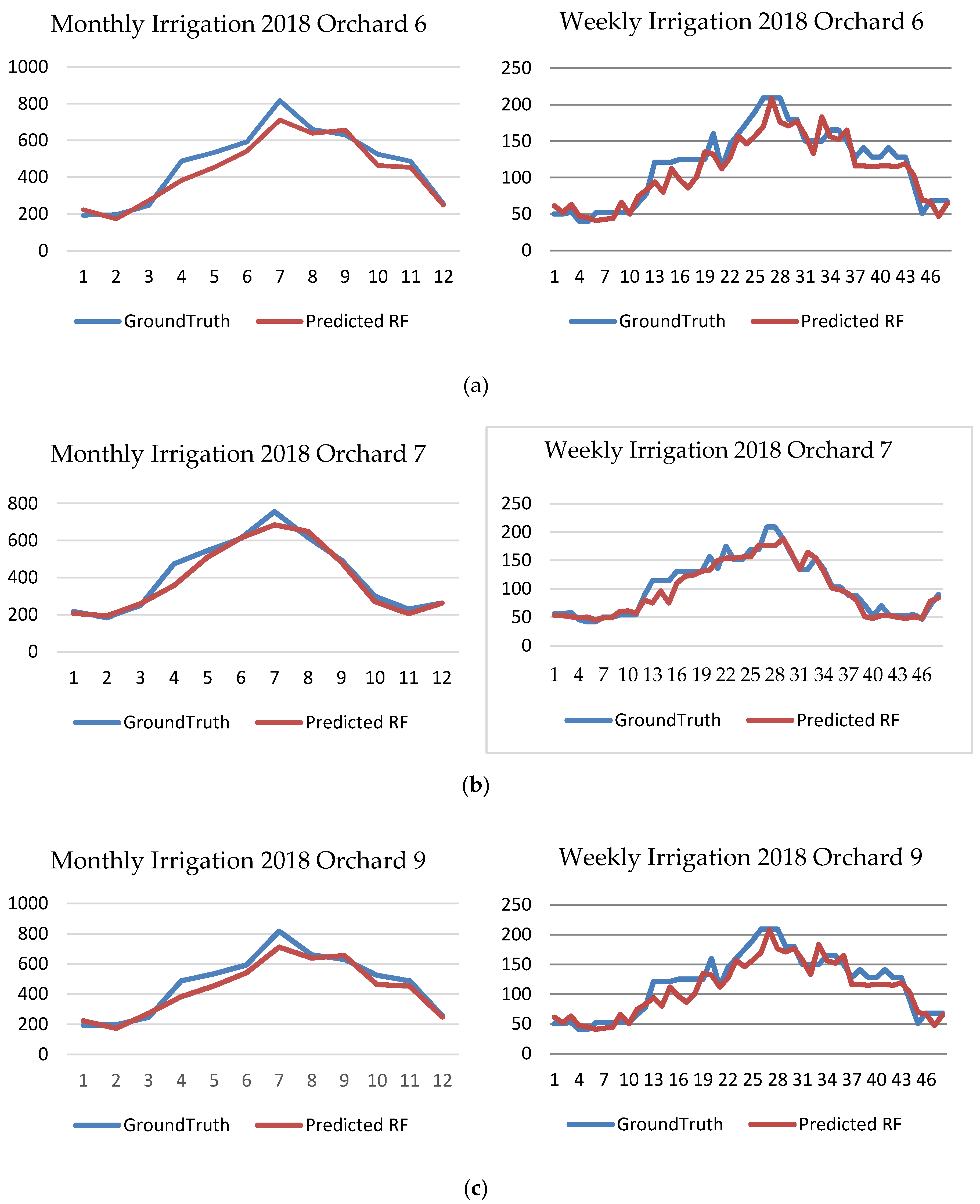
2.3.3. Regression Trees: Bagging Regression and Random Forest Regression

In the case of nonlinear and complex relationships between the features and the response, regression trees have shown better performance than classical approaches. In a regression tree, the feature space is divided into J non-overlapping “boxes,” and the prediction for a new observation is given by the mean of the response values of the training data belonging to the same “box” as the new observation.

Let $\left\{\left(x_1,y_1\right),\left(x_2,y_2\right),\dots ,\left(x_n,y_n\right)\right\}$ be the training dataset, where each $y_i$ denotes the i-th output (response variable) and $x_i = (x_{i,1}$,$x_{i,2},\dots ,x_{i,k})$ the corresponding input of the s predictors (features) in the study. The objective in a regression tree is to find boxes $B_1,B_2,\dots ,B_j$ that minimize the RSS, given by Equation (3):

$${\displaystyle \sum }_{j =1}^J{\displaystyle \sum }_{i\in B_j}^{}{\left(y_i-{\widehat{y}}_{B_j}\right)}^2$$

(3)

where ${\widehat{y}}_{B_j}$ is the mean response for the training observations within the jth box.

A desirable criterion could be to find the partition of the feature space that minimizes the residual sum of squares (RSS) for the training dataset, but this approach is usually computationally infeasible. Therefore, the way to obtain the partition of the feature space is by means of binary splitting: the algorithm chooses, at each step, the predictor ($X_j$) and cut-point (s) that minimize the RSS for the resulting tree. In general, the above optimization problem is not very computationally demanding, except when the number of features is too large. The process is repeated until a stopping criterion is reached, for instance, until all regions contain less than a determined number of observations.

Regression trees have many advantages: they are easy to explain, computationally fast to obtain, and can handle missing data, outliers, and irrelevant features. However, they are very sensitive to the data and can overfit the training data (there are lots of small branches). A way to keep from overfitting is to prune the least important leaves of the tree. Therefore, using a good strategy for pruning the tree, a single regression tree can be used as a prediction method, but it is more efficient to use them as base learners in complex solutions.

In random forest and bagging, the original training dataset is used to build N new subsets that only perform random sampling with replacement. For each new training dataset, the corresponding regression tree is developed. Given a new observation, the prediction of each single tree is computed, and the final prediction is obtained as the mean of the single predictions. The final prediction reduces the variance and improves accuracy [46].

The difference between bagging (bootstrap aggregating) and random forest is the number of predictors (features) considered at each split of the tree. In bagging, all the features are used, whereas in random forest only a random sample of mtry (predictors considered at each split of the regression tree) can be chosen each time. This last approach allows one to reduce the variance more efficiently.

The main parameters to be tuned in random forest are N and mtry, whereas for bagging only N should be tuned because mtry = k (the total number of features) is determined. It is important to highlight that, for these methods, the fitting goodness increases (or at least does not decrease) with the number of trees, so we do not have to worry about choosing values for N that are greater than necessary.

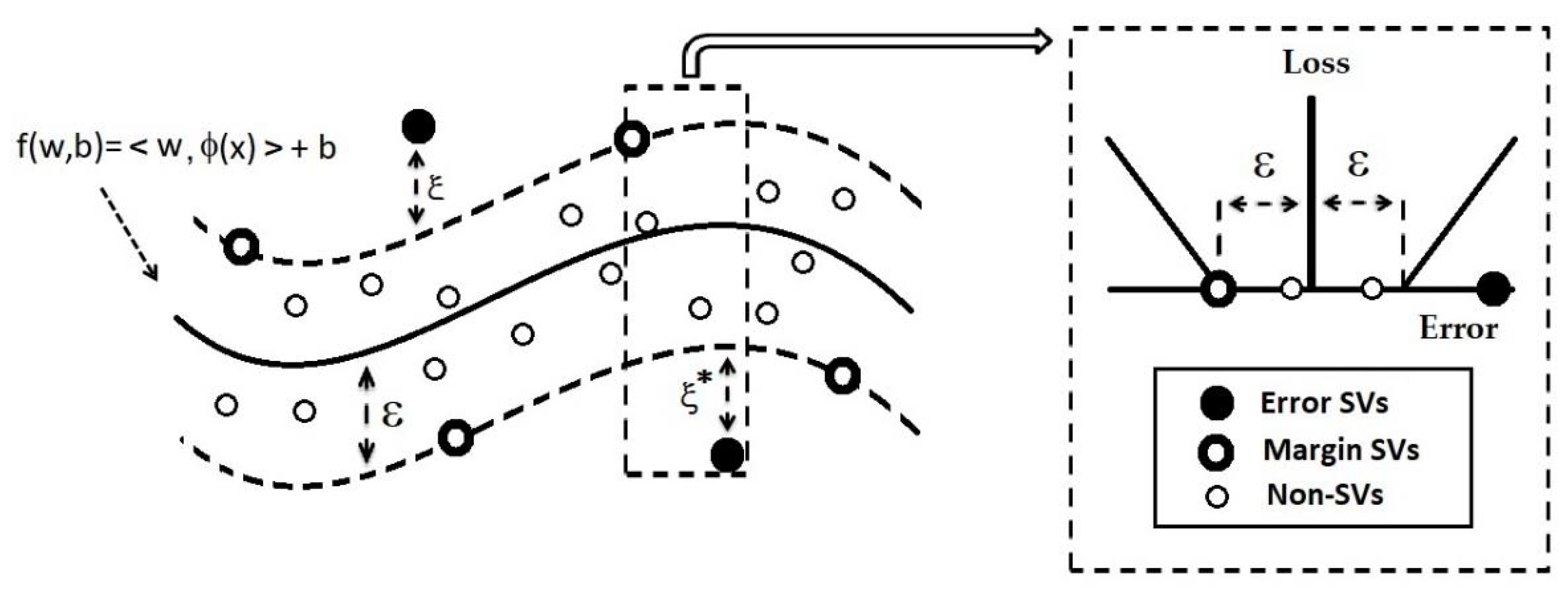
2.3.4. Support Vector Regression

Support vector machines (SVMs) are very popular in the field of classification problems. The adaptation of the SVM approach to regression problems has led to an effective tool in function estimation: SVR. In this section, the basis of the SVR technique is depicted together with suggestions for the parameter selection stage of the method. Firstly, the linear case is presented for simplicity, and the nonlinear case is introduced secondly.

The objective of the linear support vector regression (LSVR) is to find a linear function of the following form that can fit the actual output vector y (response variable) while balancing model complexity and prediction error:

$$f\left(\mathit{x}\right)=\mathit{w},\mathit{x}+b={\displaystyle \sum }_{j=1}^k{w}_j{x}_j+b, bϵR,\mathit{x},\mathit{w}ϵR^k$$

(4)

In Equation (4), $\mathit{x}$ denotes the vector of input features, k the number of features, $\mathit{w}$ the vector of parameters to be estimated, and b the position parameter to be estimated. The vector of parameters $\mathit{w}$ represents the flatness or simplicity of the function. SVM generalization to SVR is accomplished by introducing an ε-insensitive region around the function, called the ε-tube, in such a way that observations $y_i$, which lie inside the tube, lead to null errors.

For the development of the method, it is necessary to set a tolerance margin ε (penalizing only the points placed outside the ε-tube [47]) and to select a loss function (that describes the way to measure the estimation errors). There are different types of loss functions (linear, quadratic, Huber, etc.), and we can distinguish between symmetrical and asymmetrical ones. In this paper, we will focus on the Vapnik’s ε-insensitive linear loss function given by

$$L_{\epsilon }\left(\mathrm{r}\right)=\{\begin{array}{cc}0& if \left|\mathrm{r}\right|\le \epsilon \\ \left|\mathrm{r}\right|-\epsilon & otherwise\end{array}$$

(5)

Note that the loss function is only affected by the training samples that lie outside the ε-tube, which are called support vectors. Though many phenomena can be modeled by linear functions, there are many situations where the relationship between the output (response variable) and the input variables (features) is not linear.

For nonlinear functions, the data can be mapped into a higher dimensional space by means of a nonlinear function $\varphi \left(\mathit{x}\right): R^k\to R^M, M>k.$ Now the aim is to find a function of the following form that can fit the output vector y while balancing model complexity and prediction error:

$$f\left(\mathit{w},b\right)=\langle \mathit{w},\varphi \left(\mathit{x}\right)\rangle +b$$

(6)

Next, the optimization problem can be written for the nonlinear case: as

$$\begin{array}{cc}\underset{\mathit{w},b,\xi ,{\xi }^{*}}{\min }& \frac{1}{2}{\left|\right|\mathit{w}\left|\right|}^2+C{\displaystyle {\displaystyle \sum }_{i=1}^n}\left({\xi }_i+{\xi }_i^{*}\right)\\ subject to& \begin{array}{c}{y}_i-\left(\langle \mathit{w},\varphi \left(\mathit{x}\right)\rangle +b\right)\le \epsilon +{\xi }_i\\ \left(\langle \mathit{w},\varphi \left(\mathit{x}\right)\rangle +b\right)-y_i\le \epsilon +{\xi }_i^{*}\\ {\xi }_i,{\xi }_i^{*}\ge 0,i=1, 2,\cdots , n\end{array}\end{array}$$

(7)

where ${\xi }_i$, ${\xi }_i^{* }$ represent the upper and lower training errors (see Figure 4), and C is a regularization parameter that controls the model error and model simplicity trade-off. For example, large values of C give more weight to minimizing the model error.

Figure 4 shows the behavior of a nonlinear SVM [23].

The selection of an appropriate transformation $\varphi \left(\mathit{x}\right)$ is not an easy task. However, one advantage of SVR is that, in practice, the nonlinear function $\varphi \left(\mathit{x}\right)$ does not need to be used.

If we re-write the optimization problem of Equation (7) in its dual form, it can be seen that only the inner products $\varphi \left({\mathit{x}}_i\right),\varphi \left({\mathit{x}}_j\right)$ are needed. In this context, Vapnik [47] proposes the use of internal products through a “kernel trick”:

$$K\left({\mathit{x}}_i,{\mathit{x}}_j\right)=\langle \varphi \left({\mathit{x}}_i\right),\varphi \left({\mathit{x}}_j\right)\rangle$$

(8)

where K(X,Y) is a function that verifies Mercer’s theorem [47]. Therefore, the SVR technique requires the selection of ε (margin of the tube), C (regularization parameter), and the kernel function.

Some of the most used kernel functions in the context of SVR are the linear, polynomial, and sigmoid kernels.

In this paper, the radial basis function (RBF) kernel, given by Equation (9), was used, because of its good results in nonlinear relations [48].

$$K\left(x_i,x_j\right)=e^{\left(-\gamma {\left|x_i-x_j\right|}^2\right)}$$

(9)

Recall that higher values of C provide more complex models and can produce overfitting of the training data. Smaller values of C result in a simpler model but low accuracy. For this paper, the value of this parameter was selected following the indications of Mattera and Haykin [49], who propose that C should be equal to the range of the output.

The parameter ε also affects the smoothness or complexity of the model. In addition, the value of ε determines the number of support vectors. Smaller values of ε lead to higher numbers of support vectors and, therefore, a more complex learning machine. However, higher values of ε lead to a lower number of support vectors, so important information may be lost. In this work, the suggestions of Cherkassky and Ma [50] and Mattera and Haykin [49] were chosen. They propose a value of ε such that the percentage of support vectors in the regression model is around 50% of the number of samples.

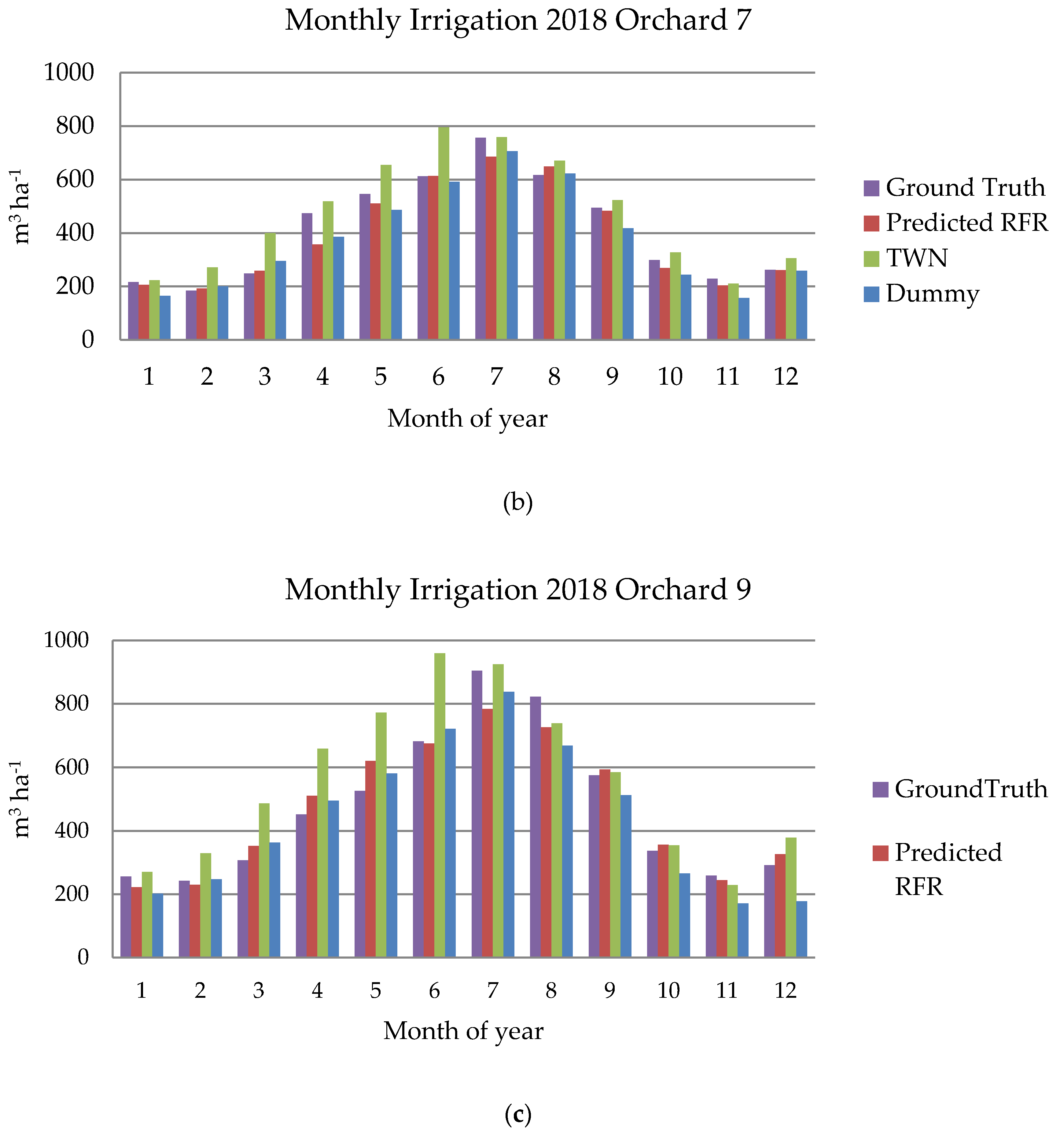
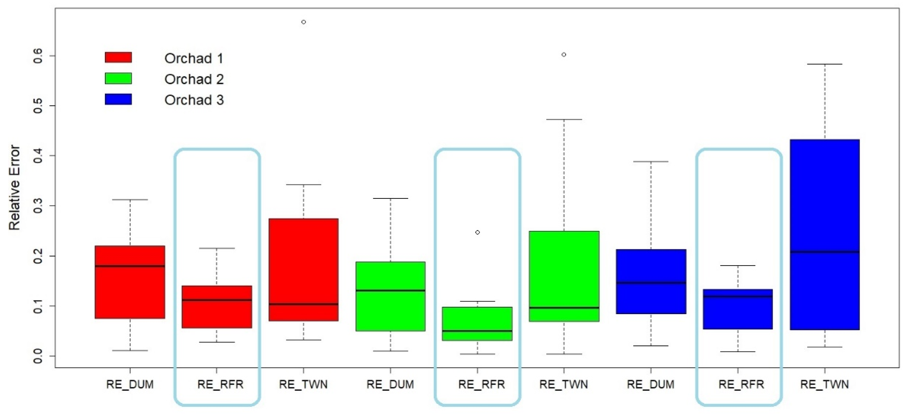
3. Results and Discussion

In this section, we show the results obtained after the training and testing stages of each regression method, and we provide different measures to compare their performances.

Regarding the LR method, the final estimated model was the same using the three selection methods (stepwise, forward, and backward).

As for the RFR method, a value of N = 500 (the total number of trees considered in the training stage) was selected, whereas mtry = 8 provided the best goodness-of-fit in the test dataset.

Finally, the SVR model that performs best uses an RBF kernel, a penalty factor C of 100, and an epsilon of 8 (obtaining 265 support vectors, which is slightly higher than 50% of the sample size).

In order to analyze the performance of the different models, LOOCV and random 90-10 shuffle cross-validation techniques were used to assure better evaluation. In both cases, the RMSE was selected as the error measure to evaluate the accuracy in the training and test datasets.

Table 2. Root-mean-square error (RMSE) of 90-10 shuffle cross-validation for the models (m³ ha⁻¹ week⁻¹). LR: linear regression; RFR: random forest regression; SVR: support vector regression.

	SVR	LR	RFR	Dummy
Train	16.7 m3	18.5 m3	6.65 m3	23.39 m3
Test	17.13 m3	19.5 m3	16.83 m3	24.85 m3

shows the results of the 90-10 shuffle cross-validation. The three regression models were compared with a dummy model that irrigates the crops based only on the TWN. This dummy model takes advantage of the fact that the maximum amount of water calculated by the agronomist is typically less than the TWN. Using the training data, the optimal percentage is calculated based on the phenological period of the crop. A value of 95% TWN is fixed in the more critical period (when the fruit is present), and 75% TWN when the fruit is not present. These values make sense according to the irrigation tips made by the agronomist.

In the case of the shuffle cross-validation, the three regression models perform much better than this dummy method. Both SVR and RFR perform similarly with RMSEs of 17.13 and 16.83 m³ ha⁻¹ in testing, respectively. LR performs worse than the other two models. It seems normal according to its linear nature that is not able to adapt well enough to more complex situations.

Table 3. RMSE of the (leave-one-out cross-validation (LOOCV) for the four models (m³ ha⁻¹ week⁻¹).

	SVR		LR		RFR		Dummy
Orchard	Train	Test	Train	Test	Train	Test	Train	Test
1	15.79	31.99	19.13	19.64	6.48	18.02	22.58	20.60
2	15.85	24.75	19.22	16.08	6.66	18.68	22.46	24. 4
3	15.11	30.48	17.59	30.87	6.29	25.53	21.30	34.25
4	15.16	23.72	18.67	26.12	6.10	24.04	22.58	20.97
5	15.04	22.17	18.78	21.90	6.41	21.32	21.79	26.44
6	15.88	15.23	19.41	16.50	6.75	13.76	23.08	18.00
7	15.33	19.70	18.88	20.01	6.48	20.06	22.62	21.74
8	16.26	11.93	19.92	10.88	6.74	14.98	23.40	16.08
9	15.59	17.43	19.03	18.95	6.51	17.84	21.71	25.46
Mean	15.55	19.99	17.95	18.35	6.49	18.01	22.39	21.71

shows the results of the LOOCV for the four prediction models and each orchard separately. The first column represents the orchard number. In this case, for each selected orchard, we do not use the data of the orchard for training—only for testing. In other words, this approach proves the generalization capabilities of the model. Each row represents the training and test errors of the models when the selected orchard is left out.

In this case, RFR is still the model that performs best, with LR in second place and performing slightly better than SVR, with average RMSE values in testing of 18.01, 18.35, and 19.99 m³ ha⁻¹ per week, respectively. All models performed better than the dummy model.

Figure 5 and

Table 4. Estimated water requirement (m³ ha⁻¹) during 2018 for each model and orchard. TWN: total water needs.

Orchard	1			2			3
Model	Dummy	RFR	TWN	Dummy	RFR	TWN	Dummy	RFR	TWN
RMSE	76.32	58.92	140.31	52.64	43.76	83.86	76.32	58.92	140.31
MRE	0.16	0.10	0.18	0.13	0.07	0.18	0.17	0.10	0.24
Total water	4860 m3	5218 m3	5912 m3	4534 m3	4690 m3	5660 m3	5242 m3	5642 m3	6684 m3
Total water ground truth	5626 m3 ha−1			4938 m3 ha−1			5635 m3 ha−1

analyze the water requirement per month for the RFR model, the dummy model, the TWN, and the GT (ground-truth) during the year 2018 and for three of the orchards. Although all nine plots were used for the model training and error comparison phases, a comparative representation of the goodness of the models with respect to GT (agronomist reports) was made for those plots for which full years of data were available, Orchards 6, 7, and 9. In this case, the relative error (RE), given in Equation (10), was used to evaluate the monthly accuracy for each prediction method:

$$RE\left(j\right) =\left|\frac{y_j-{\widehat{y}}_j}{y_j}\right|$$

(10)

where $y_j$ is the actual output for month j, and ${\widehat{y}}_j$ is the estimated output for month j. Note that this error measure is a dimensionless quantity (see Figure 6), and it does not make sense when the output variable can take null values. The mean relative error (MRE), computed as the mean of the monthly relative errors, provides a dimensionless global error measure (see Table 4):

$$MRE =\frac{{{\displaystyle \sum }}_{j = 1}^{m}RE\left(j\right)}{m}=\frac{{{\displaystyle \sum }}_{j = 1}^m\left|\frac{y_j-{\widehat{y}}_j}{y_j}\right|}{m}$$

(11)

where m denotes the number of months considered; in our case, m = 12 because the methods were evaluated just for the year 2018.

Figure 6 shows the distribution of the relative errors associated with each prediction model compared to the GT. We can notice that the RFR model has much less dispersion and fewer relative errors compared to the TWN and dummy methods.

Irrespective of the magnitude of the residuals, it is important to verify if the prediction errors behave properly (ensuring no bias, low dispersion, and symmetry). In this sense, the quality of the errors was checked, analyzing, for each prediction method, the distribution of the net residuals by means of the box plots given in Figure 7. It can be seen that the TWN and dummy methods provide higher bias, dispersion, and asymmetry than the RFR method.

In Figure 8, we can see that the monthly and weekly RFR prediction follow quite precisely the tendency of the GT for all months and weeks in each one of the three orchards tested.

4. Conclusions

This paper describes the design and development of an automatic decision support system to manage irrigation in agriculture.

The system was trained with climatic and soil data from nine different citric crops located in different zones of Southeast Spain.

The aim of the IDSS is to mimic the irrigation recommendations of an agronomist, with the idea of creating a robust model (with good generalization capabilities) able to precisely predict the weekly water requirement of the crops with no previous information of the specific field.

Three regression methods were tested to determine the one that best fits the agronomist criteria. RFR was the method that best emulated the agronomist.

Despite the results obtained among the regression models tested, the number of reports is a critical factor that directly affects the performance of the methods.

Regarding the water applied, we can conclude that considering only the TWN for irrigation wastes water (an increment of 282, 722, and 1049 m³ ha⁻¹ per year for Orchards 6, 7, and 9, respectively) compared to the agronomist. In contrast, the dummy estimator tends to heavily underestimate the water requirements (with underestimates of 766, 404, and 393 m³ ha⁻¹ for Orchards 6, 7, and 9, respectively). However, the RFR model performed much better than the others (408, 248, and 7 m³ ha⁻¹) with errors below 12% for all the orchards and weeks.

In terms of performance, considering the water predicted by the IDSS versus the agronomist, the system has a weekly average error below 9% for the most critical periods (the ones when the fruit is growing), with a 10% error being considered acceptable in agriculture. It can be concluded that the IDSS is a viable predictor [51].

For future research, we aim to extend the dataset with more citrus plantations in order to analyze the performance in different regions and weather conditions. In addition, exporting this model to other plantations different from citrus and adding data only from VWC sensors would be a good way of evaluating the robustness of the model and decreasing the cost of the whole system.

Another future improvement would be to migrate the system to daily instead of a weekly prediction. This change would vastly increase the potential of the model, as it would be able to adapt more quickly to changes in weather conditions and decrease the reaction time, which will result in water savings.

References

1. Domingo, R.; Ruiz-Sánchez, M.C.; Sánchez-Blanco, M.J.; Torrecillas, A. Water relations, growth and yield of Fino lemon trees under regulated deficit irrigation. Irrig. Sci. 1996, 16, 115–123. [Google Scholar] [CrossRef]
2. Torrecillas, A.; Alarcón, J.J.; Domingo, R.; Planes, J.; Sánchez-Blanco, M.J. Strategies for drought resistance in leaves of two almond cultivars. Plant Sci. 1996, 118, 135–143. [Google Scholar] [CrossRef]
3. Hashem, I.A.T.; Yaqoob, I.; Anuar, N.B.; Mokhtar, S.; Gani, A.; Ullah Khan, S. The rise of “big data” on cloud computing: Review and open research issues. Inf. Syst. 2015, 47, 98–115. [Google Scholar] [CrossRef]
4. Navarro-Hellín, H.; Torres-Sánchez, R.; Soto-Valles, F.; Albaladejo-Pérez, C.; López-Riquelme, J.A.; Domingo-Miguel, R. A wireless sensors architecture for efficient irrigation water management. Agric. Water Manag. 2015, 151. [Google Scholar] [CrossRef] [Green Version]
5. Gubbi, J.; Buyya, R.; Marusic, S.; Palaniswami, M. Internet of Things (IoT): A vision, architectural elements, and future directions. Futur. Gener. Comput. Syst. 2013, 29, 1645–1660. [Google Scholar] [CrossRef] [Green Version]
6. Davis, S.L.; Dukes, M.D.; Miller, G.L. Landscape irrigation by evapotranspiration-based irrigation controllers under dry conditions in Southwest Florida. Agric. Water Manag. 2009, 96, 1828–1836. [Google Scholar] [CrossRef]
7. Zhang, X.; Khachatryan, H. Investigating homeowners’ preferences for smart irrigation technology features. Water 2019, 11, 1996. [Google Scholar] [CrossRef] [Green Version]
8. Davis, S.L.; Dukes, M.D. Irrigation scheduling performance by evapotranspiration-based controllers. Agric. Water Manag. 2010, 98, 19–28. [Google Scholar] [CrossRef]
9. Gutierrez, J.; Villa-Medina, J.F.; Nieto-Garibay, A.; Porta-Gandara, M.A. Automated irrigation system using a wireless sensor network and GPRS module. IEEE Trans. Instrum. Meas. 2014, 63, 166–176. [Google Scholar] [CrossRef]
10. Campbell, J.E. Dielectric properties and influence of conductivity in soils at one to fifty megahertz. Soil Sci. Soc. Am. J. 1990, 54, 332–341. [Google Scholar] [CrossRef]
11. Visconti, F.; de Paz, J.M.; Martínez, D.; Molina, M.J. Laboratory and field assessment of the capacitance sensors Decagon 10HS and 5TE for estimating the water content of irrigated soils. Agric. Water Manag. 2014, 132, 111–119. [Google Scholar] [CrossRef]
12. Kizito, F.; Campbell, C.S.; Campbell, G.S.; Cobos, D.R.; Teare, B.L.; Carter, B.; Hopmans, J.W. Frequency, electrical conductivity and temperature analysis of a low-cost capacitance soil moisture sensor. J. Hydrol. 2008, 352, 367–378. [Google Scholar] [CrossRef]
13. Kargas, G.; Soulis, K.X. Performance evaluation of a recently developed soil water content, dielectric permittivity, and bulk electrical conductivity electromagnetic sensor. Agric. Water Manag. 2019, 213, 568–579. [Google Scholar] [CrossRef]
14. González-Teruel, J.D.; Torres-Sánchez, R.; Blaya-Ros, P.J.; Toledo-Moreo, A.B.; Jiménez-Buendía, M.; Soto-Valles, F. Design and calibration of a low-cost SDI-12 soil moisture sensor. Sensors 2019, 19, 491. [Google Scholar] [CrossRef] [PubMed] [Green Version]
15. Barker, J.B.; Franz, T.E.; Heeren, D.M.; Neale, C.M.U.; Luck, J.D. Soil water content monitoring for irrigation management: A geostatistical analysis. Agric. Water Manag. 2017, 188, 36–49. [Google Scholar] [CrossRef] [Green Version]
16. Gavilán, V.; Lillo-Saavedra, M.; Holzapfel, E.; Rivera, D.; García-Pedrero, A. Seasonal crop water balance using harmonized Landsat-8 and Sentinel-2 time series data. Water 2019, 11, 2236. [Google Scholar] [CrossRef] [Green Version]
17. Jones, H.G. Use of infrared thermometry for estimation of stomatal conductance as a possible aid to irrigation scheduling. Agric. For. Meteorol. 1999, 95, 139–149. [Google Scholar] [CrossRef]
18. García-Tejero, I.F.; Ortega-Arévalo, C.J.; Iglesias-Contreras, M.; Moreno, J.M.; Souza, L.; Tavira, S.C.; Durán-Zuazo, V.H. Assessing the crop-water status in almond (Prunus dulcis mill.) trees via thermal imaging camera connected to smartphone. Sensors 2018, 18, 1050. [Google Scholar] [CrossRef] [Green Version]
19. Jackson, R.D.; Idso, S.B.; Reginato, R.J.; Pinter, P.J. Canopy temperature as a crop water stress indicator. Water Resour. Res. 1981, 17, 1133–1138. [Google Scholar] [CrossRef]
20. Luthra, S.K.; Kaledhonkar, M.J.; Singh, O.P.; Tyagi, N.K. Design and development of an auto irrigation system. Agric. Water Manag. 1997, 33, 169–181. [Google Scholar] [CrossRef]
21. Panigrahi, P.; Raychaudhuri, S.; Thakur, A.K.; Nayak, A.K.; Sahu, P.; Ambast, S.K. Automatic drip irrigation scheduling effects on yield and water productivity of banana. Sci. Hortic. (Amsterdam). 2019, 257. [Google Scholar] [CrossRef]
22. Osroosh, Y.; Troy Peters, R.; Campbell, C.S.; Zhang, Q. Automatic irrigation scheduling of apple trees using theoretical crop water stress index with an innovative dynamic threshold. Comput. Electron. Agric. 2015, 118, 193–203. [Google Scholar] [CrossRef]
23. Field Comparison of Tensiometer and Granular Matrix Sensor Automatic Drip Irrigation on Tomato in: HortTechnology Volume 15 Issue 3 (2005). Available online: https://journals.ashs.org/horttech/view/journals/horttech/15/3/article-p584.xml (accessed on 3 December 2019).
24. Cáceres, R.; Casadesús, J.; Marfà, O. Adaptation of an automatic irrigation-control tray system for outdoor nurseries. Biosyst. Eng. 2007, 96, 419–425. [Google Scholar] [CrossRef]
25. Bacci, L.; Battista, P.; Rapi, B. An integrated method for irrigation scheduling of potted plants. Sci. Hortic. (Amsterdam) 2008, 116, 89–97. [Google Scholar] [CrossRef]
26. Casadesús, J.; Mata, M.; Marsal, J.; Girona, J. A general algorithm for automated scheduling of drip irrigation in tree crops. Comput. Electron. Agric. 2012, 83, 11–20. [Google Scholar] [CrossRef]
27. Puerto, P.; Domingo, R.; Torres, R.; Pérez-Pastor, A.; García-Riquelme, M. Remote management of deficit irrigation in almond trees based on maximum daily trunk shrinkage: Water relations and yield. Agric. Water Manag. 2013, 126, 33–45. [Google Scholar] [CrossRef]
28. Li, M.; Sui, R.; Meng, Y.; Yan, H. A real-time fuzzy decision support system for alfalfa irrigation. Comput. Electron. Agric. 2019, 163. [Google Scholar] [CrossRef]
29. Li, H.; Li, J.; Shen, Y.; Zhang, X.; Lei, Y. Web-based irrigation decision support system with limited inputs for farmers. Agric. Water Manag. 2018, 210, 279–285. [Google Scholar] [CrossRef]
30. Giusti, E.; Marsili-Libelli, S. A fuzzy decision support system for irrigation and water conservation in agriculture. Environ. Model. Softw. 2015, 63, 73–86. [Google Scholar] [CrossRef]
31. Pluchinotta, I.; Pagano, A.; Giordano, R.; Tsoukiàs, A. A system dynamics model for supporting decision-makers in irrigation water management. J. Environ. Manage. 2018, 223, 815–824. [Google Scholar] [CrossRef]
32. Rupnik, R.; Kukar, M.; Vračar, P.; Košir, D.; Pevec, D.; Bosnić, Z. AgroDSS: A decision support system for agriculture and farming. Comput. Electron. Agric. 2018. [Google Scholar] [CrossRef]
33. Goap, A.; Sharma, D.; Shukla, A.K.; Rama Krishna, C. An IoT based smart irrigation management system using Machine learning and open source technologies. Comput. Electron. Agric. 2018, 155, 41–49. [Google Scholar] [CrossRef]
34. Goldstein, A.; Fink, L.; Meitin, A.; Bohadana, S.; Lutenberg, O.; Ravid, G. Applying machine learning on sensor data for irrigation recommendations: Revealing the agronomist’s tacit knowledge. Precis. Agric. 2018, 19, 421–444. [Google Scholar] [CrossRef]
35. Rose, D.C.; Sutherland, W.J.; Parker, C.; Lobley, M.; Winter, M.; Morris, C.; Twining, S.; Ffoulkes, C.; Amano, T.; Dicks, L.V. Decision support tools for agriculture: Towards effective design and delivery. Agric. Syst. 2016, 149, 165–174. [Google Scholar] [CrossRef] [Green Version]
36. Navarro-Hellín, H.; Martínez-del-Rincon, J.; Domingo-Miguel, R.; Soto-Valles, F.; Torres-Sánchez, R. A decision support system for managing irrigation in agriculture. Comput. Electron. Agric. 2016, 124. [Google Scholar] [CrossRef] [Green Version]
37. Nawandar, N.K.; Satpute, V.R. IoT based low cost and intelligent module for smart irrigation system. Comput. Electron. Agric. 2019, 162, 979–990. [Google Scholar] [CrossRef]
38. Romero, M.; Luo, Y.; Su, B.; Fuentes, S. Vineyard water status estimation using multispectral imagery from an UAV platform and machine learning algorithms for irrigation scheduling management. Comput. Electron. Agric. 2018, 147, 109–117. [Google Scholar] [CrossRef]
39. Yamaç, S.S.; Todorovic, M. Estimation of daily potato crop evapotranspiration using three different machine learning algorithms and four scenarios of available meteorological data. Agric. Water Manag. 2020, 228. [Google Scholar] [CrossRef]
40. Kisi, O. Modeling reference evapotranspiration using three different heuristic regression approaches. Agric. Water Manag. 2016, 169, 162–172. [Google Scholar] [CrossRef]
41. Tang, D.; Feng, Y.; Gong, D.; Hao, W.; Cui, N. Evaluation of artificial intelligence models for actual crop evapotranspiration modeling in mulched and non-mulched maize croplands. Comput. Electron. Agric. 2018, 152, 375–384. [Google Scholar] [CrossRef]
42. Feng, Y.; Cui, N.; Gong, D.; Zhang, Q.; Zhao, L. Evaluation of random forests and generalized regression neural networks for daily reference evapotranspiration modelling. Agric. Water Manag. 2017, 193, 163–173. [Google Scholar] [CrossRef]
43. SIAM—Sistema de Información Agraria de Murcia. Available online: http://siam.imida.es/apex/f?p=101:1:699166260304082 (accessed on 3 April 2019).
44. San-Segundo, R.; Navarro-Hellín, H.; Torres-Sánchez, R.; Hodgins, J.; de la Torre, F. Increasing robustness in the detection of freezing of gait in Parkinson’s disease. Electronics 2019, 8, 119. [Google Scholar] [CrossRef] [Green Version]
45. Blanco, V.; Domingo, R.; Pérez-Pastor, A.; Blaya-Ros, P.J.; Torres-Sánchez, R. Soil and plant water indicators for deficit irrigation management of field-grown sweet cherry trees. Agric. Water Manag. 2018, 208. [Google Scholar] [CrossRef]
46. James, G.; Witten, D.; Hastie, T.; Tibshirani, R. An Introduction to Statistical Learning; Springer: Berlin, Germany, 2013; ISBN 978-1-4614-7137-0. [Google Scholar]
47. Vapnik, V.N. An overview of statistical learning theory. IEEE Trans. Neural Networks 1999. [Google Scholar] [CrossRef] [PubMed] [Green Version]
48. Ghosh, S. SVM-PGSL coupled approach for statistical downscaling to predict rainfall from GCM output. J. Geophys. Res. Atmos. 2010. [Google Scholar] [CrossRef] [Green Version]
49. Mattera, D.; Haykin, S. Support vector machines for dynamic reconstruction of a chaotic system. In Advances in Kernel Methods: Support Vector Learning; The MIT Press: Cambridge, MA, USA, 1998. [Google Scholar]
50. Cherkassky, V.; Ma, Y. Practical selection of SVM parameters and noise estimation for SVM regression. Neural Netw. 2004. [Google Scholar] [CrossRef] [Green Version]
51. Bos, M.G.; Burton, M.A.; Molden, D.J. Irrigation and Drainage Performance Assessment: Practical Guidelines; CABI Publishing: Oxfordshire, UK, 2005; ISBN 0851999670. [Google Scholar]
Figure 1. Process used by the agronomist to determine irrigation dose and frequency.
Water 12 00548 g001
Figure 2. (a) Soil matric potential sensor MPS6. (b) Soil water content sensor 10HS. (c) Soil water content, temperature, and electrical conductivity (EC) sensor 5TE. (d) Water flow meter device JS04.
Water 12 00548 g002
Figure 3. Climatic stations belonging to SIAM placed in diverse locations in the region of Murcia.
Water 12 00548 g003
Figure 4. Nonlinear support vector regression (SVR) with Vapnik’s ε-insensitive loss function.
Water 12 00548 g004
Figure 5. Monthly estimated water requirement for the year 2018: (a) Orchard 1; (b) Orchard 2; (c) Orchard 3.
Water 12 00548 g005aWater 12 00548 g005b
Figure 6. Relative error (RE) distribution for each of the monthly model predictions for the year 2018.
Water 12 00548 g006
Figure 7. Distribution of the residuals (net errors) for the dummy, RFR, and TWN prediction methods.
Water 12 00548 g007
Figure 8. Comparison between the irrigation applied by the expert (ground-truth) and the one predicted by the RFR model for the year 2018: (a) Orchard 1; (b) Orchard 2; (c) Orchard 3.
Water 12 00548 g008