Bathymetry Time Series Using High Spatial Resolution Satellite Images
by
 , , , and
Manuel Erena
1,* ,
,
José A. Domínguez
1, 
Joaquín F. Atenza
1,
Sandra García-Galiano
2,
Juan Soria
3 and
and
Ángel Pérez-Ruzafa
4
1
GIS and Remote Sensing, Murcia Institute of Agri-Food Research and Development, C/Mayor s/n, La Alberca, 30150 Murcia, Spain
2
Department of Mining and Civil Engineering, Universidad Politécnica de Cartagena, 30203 Cartagena Spain
3
Instituto Cavanilles de Biodiversidad y Biología Evolutiva, Universidad de Valencia, 46980 Paterna, Spain
4
Department of Ecology and Hydrology, University of Murcia, 30100 Murcia, Spain
*
Author to whom correspondence should be addressed.
Water 2020, 12(2), 531; https://doi.org/10.3390/w12020531
Submission received: 20 December 2019
/
Revised: 3 February 2020
/
Accepted: 4 February 2020
/
Published: 14 February 2020
(This article belongs to the Special Issue Study of Lagoons and Other Shallow Water Bodies Through the Application of Numerical Models)
Abstract
:The use of the new generation of remote sensors, such as echo sounders and Global Navigation Satellite System (GNSS) receivers with differential correction installed in a drone, allows the acquisition of high-precision data in areas of shallow water, as in the case of the channel of the Encañizadas in the Mar Menor lagoon. This high precision information is the first step to develop the methodology to monitor the bathymetry of the Mar Menor channels. The use of high spatial resolution satellite images is the solution for monitoring many hydrological changes and it is the basis of the three-dimensional (3D) numerical models used to study transport over time, environmental variability, and water ecosystem complexity.
1. Introduction
The issues of hydro-sedimentary processes in lagoons, estuaries, and enclosed bays are important in terms of coastal management, because they are generally characterized by a strong human presence that results in the release of contaminants and large quantities of nutrients into the ecosystem [1]. There are many methodologies to study the nutrients in ecosystems; one of them, possibly the most used, is the three-dimensional (3D) numerical model.
The use of numerical models as a tool to anticipate the effects of human impacts or climate change effects on marine ecosystems has increased in the last decade. They permit to simulate hydrodynamic process, tides, currents, wave action, sediment transport, pollutant dispersal or biological connectivity. A large list of models is available, like CSIRO [2], Delft3D-FLOW [3,4], MARS3D [5], MIKE 21/3 [6]; MIKE3 [7], MOHIDWater [8], 3D-MOHID [9], NHWAVE [10], REF-DIF1 [11], ROM [12,13], SELFE [14,15], SCHISM [16,17], SHYFEM [18,19], SHORECIRC [20], SWAN [21] or TELEMAC [22]. Some of these models are mainly applied to shallow coastal waters. A synthesis of concepts and recommendations for model selection, mainly applied to coastal lagoons modelling, is presented by [23].
In the Mar Menor lagoon, ROMS has been used to evaluate the water renewal conditions, and a time series spanning a period longer than one year (between 2010 and 2012) provides a record of the seasonal variability of the lagoon hydrodynamics, which was used to validate the hydrodynamic model implemented [24]. SHYFEM has been used to compare the water exchange and mixing in 10 Mediterranean lagoons (including the Mar Menor) in terms of water exchange and mixing behavior. The authors found that the exchange with the open sea highly influenced the transport time scales, although the wind can also enhance the exchange mechanisms in lagoons with more than one inlet [18]. The SHYFEM has been more specifically used for the Mar Menor lagoon under different dredging scenarios of the inlets, covering different dredging depths and extensions. From this study, it can be concluded that the impacts of dredging the channels on the hydrodynamics of a coastal lagoon increase with the magnitude of the dredging activities. In this sense, there is a threshold for the magnitude of these activities beyond which important environmental effects can be expected [25,26]. Additionally, the SHYFEM has been used to model environmental parameters such as salinity and temperature [26] as well as the connectivity between the Mar Menor lagoon and the Mediterranean using a Lagrangian model [27,28], so as for predicting the effects of climate change [29].
The 3D numerical models need precise and updated initial conditions (Xo, Yo, Zo) to run them [1]. In all the cases, but mainly for applications in coastal zones, the applicability and usefulness of the results are highly dependent on the quality and spatial resolution of the bathymetric information and model grid setup, which determines not only the water column depth, but also information on bed roughness and the incorporation of specific structures and features that affect water and sediment transport dynamics. Furthermore, although the numerical models are very reliable, bottom conditions are dynamic and can change due to natural dynamics, human activities, disasters induced by cut-off lows (CoLs), such as flooding [30], and changing of the coastline [31]. Therefore, it is crucial to regularly update the information and to improve both the accuracy of bathymetric measurements and the interpolation techniques to build high-resolution grids [32,33,34,35,36].
One of the approaches to get extensive bathymetric information in inland and coastal water masses with an increasing spatial resolution is developing different tools based in remote sensing techniques [37,38,39,40,41].
In several places around the world, the CoLs contribute to increases in precipitation and in extreme rainfall events [42]. In Spain, this atmospheric phenomenon has been known traditionally as the “gota fría”, and also recently (due to the influence of meteorologists) as “dana”; both refer to CoLs. In recent years, CoLs have become more frequent in South East (SE) Spain and they are modifying the morphology of the coastline as well as the depth, seagrass, and bottom of aquatic ecosystems, particularly of the Mar Menor lagoon. An upgrade was designed to update the depth data and thus maintain the accuracy of the 3D numerical models, using the best techniques already available [43] or in development [44].
During the last semester of 2019, there were two CoLs over the Spanish Mediterranean coast that caused environmental disasters and human life loss.
Remote sensing has been used to monitor these environmental disasters [45]. Besides, remote sensing can also show the initial conditions in unaffected areas where the water is clear and the energy from the sun reaches the bottom. The energy in the water reaches the optical sensor placed above the water. The relationship between the water-leaving reflectance just above the surface and the water-leaving reflectance just below the surface is constant [46,47,48]. If the water is clear, the energy arrives from the bottom through the water column [49], in this case it is possible to determinate the water depth. The use of high-resolution satellite imagery over variable bottom types has allowed the determination of water depth with a new algorithm, which uses the relation between the neperian algorithms of two bands. The influence of the bottom is determined by a simple model, in which the bottom optical properties and the water optical properties are included [50,51]. It is noteworthy that the first studies on water depth by remote sensing in the 1970s were by simple regression methods with one band or multiple regression methods using two bands [52,53,54]. The second stage was to assess the influence of different types of bottom [55]. On the other hand, the water depth using passive optical sensors were compared with depth water obtained from LiDAR data [56]. According to the potential of the remote sensing, the images from different sensors have been used to determinate the bathymetric maps: Landsat 5 [57,58], Landsat 7 [59,60], Landsat 8 [61,62], ASTER [63], IKONOS [64], Worldview 2 [65], SPOT-4 [66], GeoEye-1 [67], and Pleiades [68]. In previous works carried out in the Mar Menor lagoon, this approach using remote sensing has been used to calculate the extinction coefficient of light (K). Then, after demonstrating its spatial heterogeneity, it was used to determine the concentration of chlorophyll a in the water column in shallow areas where the reflectance from the benthic meadows interferes with the signal of the water column [69]. Therefore, the calibration of the model requires field information provided by sounding equipment installed in ships, which cannot measure depths of less than 0.6 m [67]. In the last few years this limitation has been overcome due to the use of an Unmanned Surface Vehicle (USV) [64], which provides data from depths of just a few centimeters. The images from new sensors in satellites [70,71], planes, and new platforms (such as drones) have provided new and better tools for the management of coastal areas since the 1980s [72]. All remote sensing advances, tools, and techniques have been evaluated so that they can be adapted to new scenarios and to water management necessities [73,74,75]. However, the management of each water body has specific problems that have to be analyzed in terms of the local conditions in order to get the best results in the least possible time. Often, it is very difficult to provide solutions because there is not enough information, above all when studying areas such as the one that concerns us, with great human and environmental pressure. Good management needs a fast and efficient methodology as the basis for prediction models in near real-time, such as the monitoring Mar Menor geoportal in near real-time. In any case, the first step is to get good and precise initial data to feed the prediction models. Therefore, the aim of the present work is the use of high and very high-resolution spatial data, as well as time series, to assess the sand movement and volume of shallow water in natural channels that connect the Mar Menor lagoon and the Mediterranean Sea.
2. Study Area and Materials
2.1. Study Area
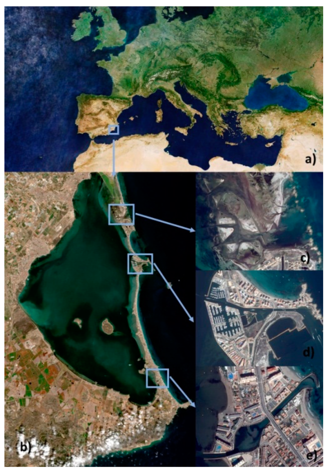
The Mar Menor is a hypersaline lagoon with a surface area of 135.76 km2, a volume of about 0.65 × 10⁹ m3, and a maximum depth of 7 m—located in the SE of the Iberian Peninsula, between the parallels 37°38′ and 37°50′ North latitude and the meridians 0°43′ and 0°57′ West longitude. There are five open channels or “golas” connecting the Mar Menor lagoon and the Mediterranean Sea. These can be seen in Figure 1c. The Encañizadas area is located at the north end of La Manga, on the southern edge of the Salinas de San Pedro Regional Park, and is made up of a group of small islets, surrounded by large flooded areas crossed by a network of shallow channels. Due to its morphology, it experiences periodic waterlogging related to tidal flows and changes in atmospheric pressure; historically, its topography and hydrology have been modified for the conditioning of fishing apparatus, known as “Encañizada”. Currently, there are three open inlets (El Ventorrillo, La Torre, and El Charco) and one channel closed by a floodgate since 1980 (New); the Estacio channel was an ancient “Encañizada” drained for the construction of the port of Tomas Maestre in 1973 and is currently the deepest (5 m; Figure 1d); and the Marchamalo channel was an old artificial “Encañizada” that never worked due to its tendency to fill with sediments (Figure 1e) [76]. Currently, it is a navigable but has a shallow channel (1 m).
The Mar Menor lagoon was created by a sequence of consecutive oscillations of the sea level that occurred in the Quaternary. It is located at the bottom of a river basin bordered by mountains that enclose the Campo de Cartagena, a vast plain of 1350 km2 with a low inclination to the SE. The contribution of continental water is made up of six watercourses, which are dry most of the year and contribute to the natural process of filling the Mar Menor lagoon [77]. In relation to this, the most outstanding geomorphological elements determining the dynamics of the lagoon are the sand barrier, continuous shore, islands and volcanic outcrops, and underwater area of the Mar Menor lagoon [77,78].
The erosion factors are mainly natural driving forces—winds, storms, waves, and a rise in sea level. The sand barrier was created by marine currents and the effect of the wind and waves. This effect is the reason why the Encañizada gola bottom is moving and changing [25,79]. The exchange between Mediterranean and lagoon waters can be affected because of changes in the inlet’s geomorphology, and these changes can affect the biological productivity, the species richness, and the complexity of the lagoon communities [80,81,82], and, therefore, affecting the environmental and economic balance of this area. Precise knowledge of the spatio-temporal evolution of the opening of this golas is very useful to improve the results of the hydrodynamic models that are being implemented for the Mar Menor lagoon and its connection with the Mediterranean Sea. According to the work of the Technical University of Cartagena (UPCT) [24], the “El Estacio” channel is the most important in the regulation of the water exchange of the Mar Menor lagoon, since it accounted for 60% of the total annual volume interchanged at that time (2010–2011), while the “Encañizadas” channel contributed 33% and the “Marchamalo” channel the remaining 7%. However, the Encañizadas can account for up to the 80% if the net balance is considered [25]. These percentages have significant seasonal fluctuations depending on the sand deposits caused by the storms in the area and the maintenance work that is carried out regularly on the golas. The water renewal rate of the volume of the Mar Menor lagoon has been calculated as 318 days [27], although this can be very variable depending on the weather conditions and freshwater inputs due to runoff or groundwater discharge [83].
2.2. In Situ Depth Data Points Obtained Using an Unmanned Surface Vehicle (USV)
The Murcia Institute of Agri-Food Research and Development (IMIDA) is working with two types of USV, developed with different aims: An Unmanned Surface Water Vehicle (USWV) to study bathymetry in shallow water, and a Remotely Operated Underwater Vehicle (ROV) to study water quality and the lagoon bottom.
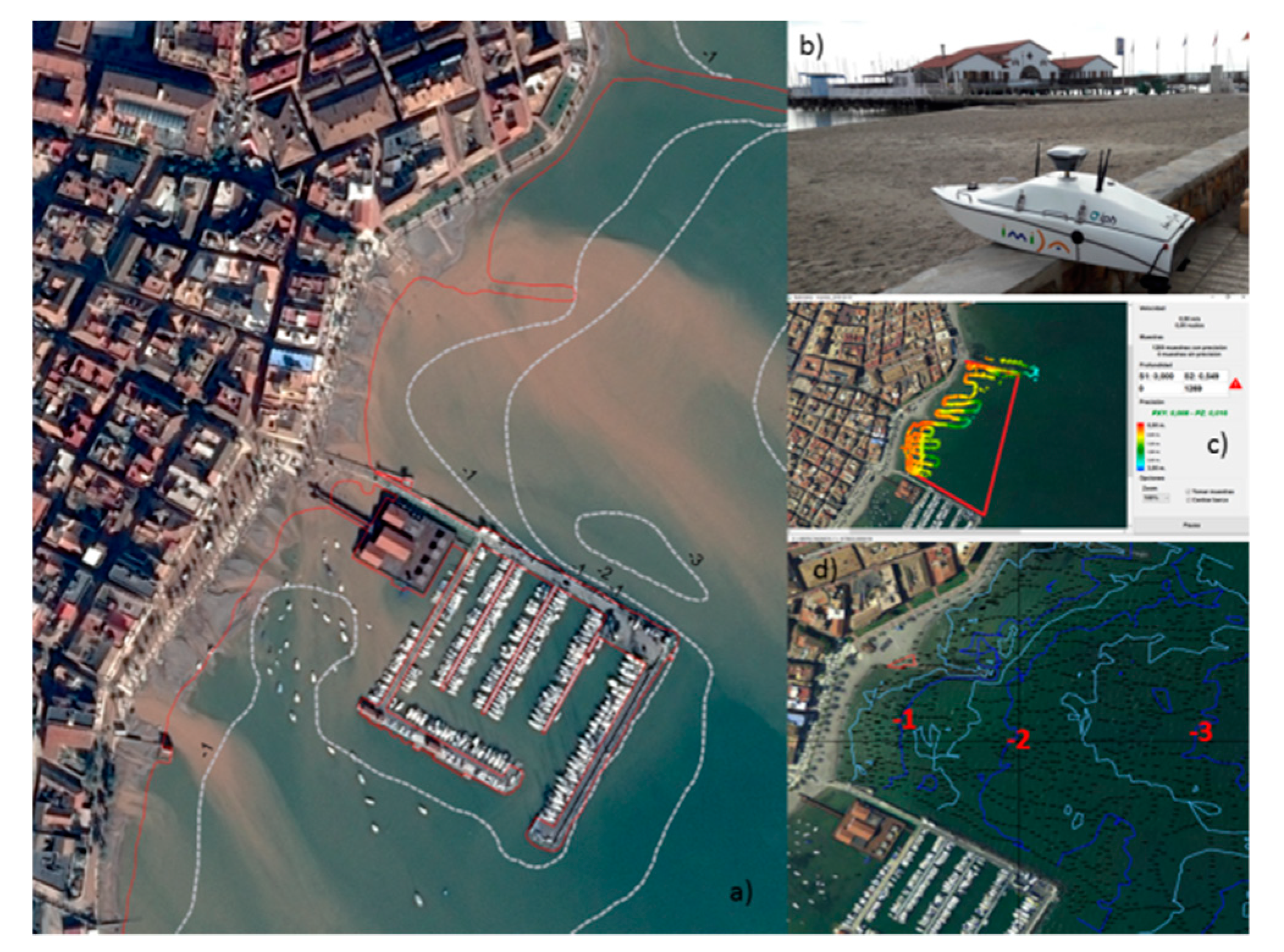
These drones are based on ArduPilot or ArduPilotMega (APM). The latter is an autopilot of free code used in the control of several types of drones, such as unmanned helicopters, unmanned aircraft, and unmanned aquatic vehicles. In recent years, more and more unmanned automatic data acquisition equipment has been applied to ocean observation, and the USWV is one example. Due to its high degree of automation and flexibility, it can be applied to the surveying and mapping of water depth. The Massachusetts Institute of Technology has developed a prototype ARTEMIS [84]; it is a small unmanned sounding vessel used in water-depth measurement. This idea has been developed into different types of small unmanned ships, boats, or catamarans [85,86,87], such as the IMIDA06 USV [88] used in this study (Figure 2).
The drones were used to perform the bathymetric work in five coastal areas of the Mar Menor lagoon and in the three channels of communication with the Mediterranean Sea (Figure 3). Special attention was given to the Encañizadas channel, where seven bathymetries have been performed in the last 10 years by different Spanish organizations (Table 1): Instituto Hidrográfico de la Marina (IHM), Ministerio de Agricultura, Pesca y Alimentación (MAGRAMA), Instituto Español de Oceanografía (IEO), UPCT and IMIDA.
2.3. Satellite Data
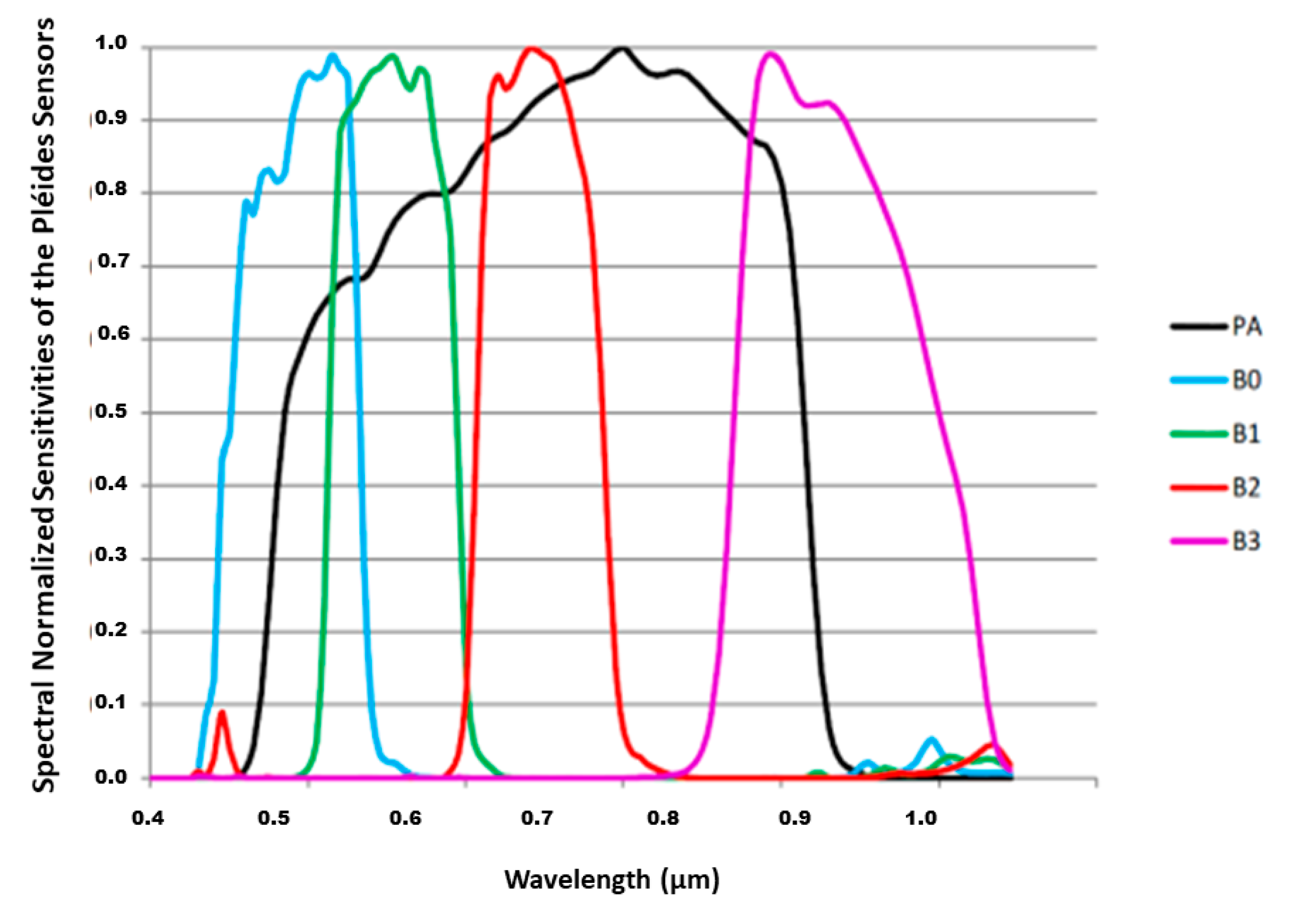
The images used in this work were provided by Airbus (Table 2) and correspond to the Pleiades satellites successfully launched on 16 December 2011. These are two optical satellites: Pleiades-1A and Pleiades-1B. Their orbits are differentiated by a 180° separation and they work together to provide daily images from anywhere on the planet. The Pleiades sensors have a nominal swath width of 20 km at nadir and two spectral configurations (Figure 4): a panchromatic configuration, with a spatial resolution of 0.5 m, and a multispectral configuration: visible (VI) and near infrared (NIR), both with a spatial resolution of 2 m.
The physical model used in this project (Appendix A) is based in the premise that the relationship between the water-leaving reflectance just above the surface R(0+,λ) and the water-leaving reflectance just below the surface R(0−,λ) is constant. The water-leaving reflectance just below the surface is a lineal combination reflectance from the water column and reflectance from the bottom. The water is clear; thus, the energy arrives from the bottom through the water column and the water column is homogenous [89]. The relationship between the water-leaving reflectance and the depth is
where m and n do not vary with depth (they are constant when the properties of the water column and the bottom are constant, too), but RBlue and RGreen do vary [60,90], since they are the reflectances below the surface with bottom influence and the reflectance below the surface without bottom influence (that is, in deep water), respectively.
2.4. LiDAR Data
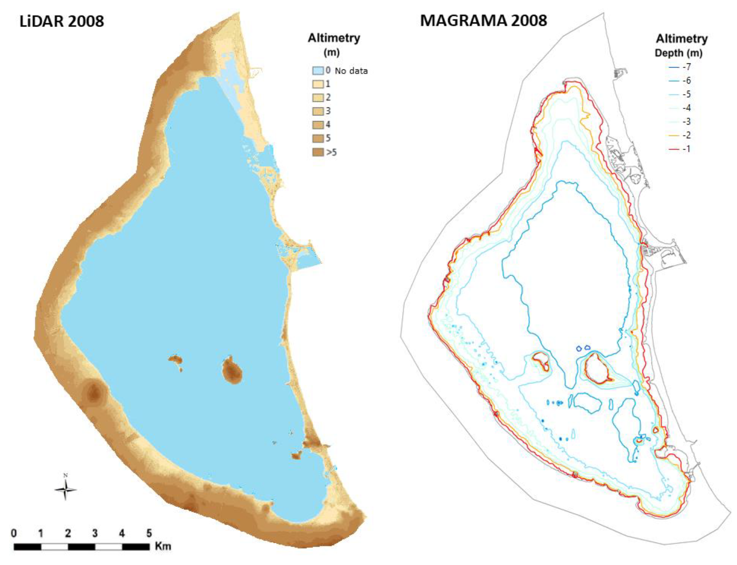
The airborne laser imaging detection and ranging (LiDAR) data correspond to the Spanish National Plan of Aerial Orthophotography (PNOA) of 2009 and 2016, of the Spanish National Geographic Institute (IGN). A model ALS50 (Leica Geosystems AG, Heerbrugg, Switzerland) was used, with a low point density (0.5 points/m2) but completely covering the Mar Menor lagoon. A digital surface model (DSM) was obtained by triangulation at a spatial resolution of 2 m. The LiDAR data (Figure 5 and Figure 6) were processed with LAStools (Rapidlasso GmbH, Gilching, Germany) and ArcGiS 10.7 (ESRI, Redlands, CA, USA) software.
2.5. Echosounder Data (2008/2009 MAGRAMA and 2016/2017 IEO and IHM)
Until 2016, for the Mar Menor lagoon there was only a single bathymetry, performed by the IHM in 1967 and published in the nautical chart No. 471A; this bathymetry was obtained with a single-beam probe. Subsequently, in 2008/2009, the Ministry of Agriculture, Fisheries, and Food performed the ultrasound mapping of the coast of the Region of Murcia (Figure 5, Supplementary Materials S1), using a Seabat 8124 multi-beam sonar systems (Reson Ltd., Slangerup, Denmark).
In order to obtain a detailed bathymetry of the seabed of the Mar Menor lagoon, the IEO and IHM carried out a data collection campaign from 26 April to 13 June 2017. The objective of this was to conduct a bathymetric analysis of the interior of the Mar Menor lagoon (at depths > 3 m) and a characterization of the seabed (Figure 6) with the GeoSwath 500 Plus interferometric probe (Kongsberg Gruppen ASA, Kongsberg, Norway), with lateral scan sonar registers by IEO [43].
3. Methodology
3.1. Ground-Based Data
During the field experiment, the IMIDA06 USV (Figure 2) used a sounding AIRMAR (Airmar Technology Corporation, Milford, CT, USA), a bi-frequency of 50/200 kHz, 600 W of power, and a GNSS receiver that synchronously collected water depth and position data with high accuracy. The GNSS RTK receiver was a GPS-GALILEO-GLONASS type and the horizontal positioning (for a Real Time Kinematic, RTK, model) was connected to the sounding data to get good depth and position data. Bathymetry is defined as the depth from the bottom to the zero value. In Spain (Royal Decree 1071/2007 Spanish law), the zero value is the sea surface in Alicante city (Spain). The measuring range is 0.5 m to 100 m and the accuracy is ±10 mm. The GNSS receiver was an Emlid Reach RS model (Emlid Ltd., Hong Kong, China), the horizontal positioning accuracy (in the RTK model) was about 10 mm, and the vertical positioning accuracy about 20 mm. The USV was developed by Inntelia (IPH Ltd., Huelva, Spain). Table 3 presents the specifications of USV components.
In the bathymetries of the three golas of December 2019, a floating drone was used with an Echologger ECT400S (EofE Ultrasonics Ltd., Kyounggi-Do, Korea), acoustic frequency of 450 kHz, sampling frequency of 100 kHz, width of the conical beam 5° (±3 dB), precision of 1 mm, a receiver and GNSS RTK antenna (GPS, GALILEO, and GLONASS), as well as lithium polymer battery power. It was controlled manually with a UHF Radio Modem system with 1 W of power (+30 dBm) for connection and data transmission. The coordinates of the ground control points (GCP) were acquired through a traditional technique, by means of a Leica-Geosystems Station TPS1200 (Leica Geosystems AG, Hauptsitz, Heerbrugg, Switzerland).
3.2. Remote Sensing Data Processing
3.2.1. Pre-Processing
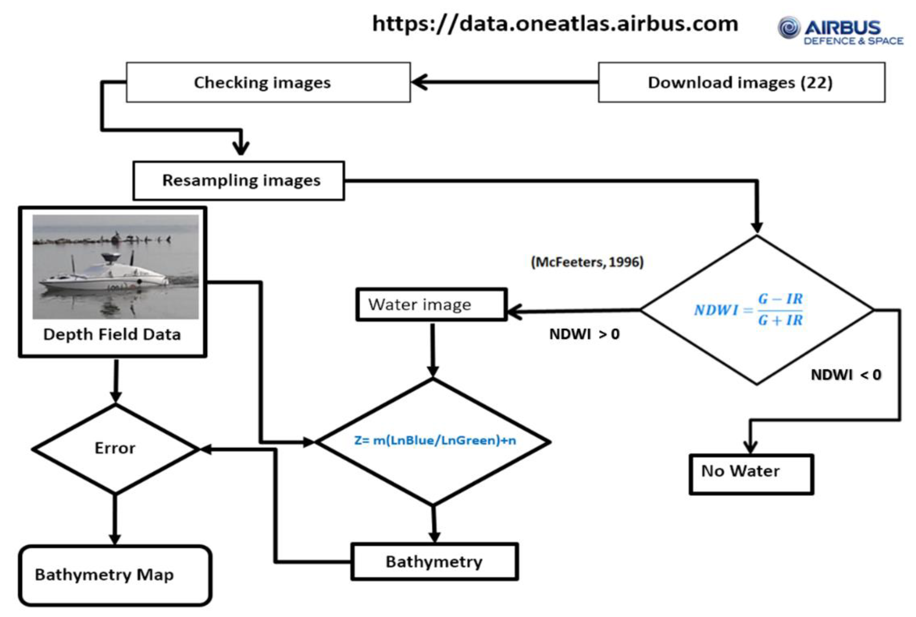
Firstly, all images available were checked on OneAtlas (Airbus DS Geo, Toulouse, France); secondly, the decoding was done (Figure 7). Each type of image was downloaded applying a specific pre-processing (Table 2). The first step finished when all images had been pre-processed. In remote sensing imagery, atmospheric correction can remove the atmospheric influence (mainly caused by atmospheric molecules and light scattering particles) and illumination factors. The target reflectance spectrum after correction will be similar to the ground-measured spectra [90,91,92].
3.2.2. Water Area
The water mask was generated using the normalized difference water index (NDWI), using green and infrared bands [93] in each reflectance image. From Figure 7, if NDWI is higher than 0, the pixel is water and if NDWI is less than 0, it is not water. Each water mask was applied to its reflectance image and all reflectance water images were obtained.
3.2.3. Water Depth Extraction Model
Reflectance water images near in time to the bathymetric data were chosen to get linear algorithms [90]. The operations between bands were performed using ENVI 4.8 software. The relationship between the raster data and the sounding data was processed with ArcMap 10.7. The m and n values of the model were obtained by EXCEL software, as well as the statistical study. The bathymetry derived from satellite data was compared with the bathymetric obtained from field data, and the normalized root mean square error (RMSE) was analyzed.
3.2.4. Bathymetric Map and Water Amount Time Series Derived from Satellite Data
The bathymetry on each date was calculated using a water depth extraction model, and the water amount was obtained by multiplying the pixel size by the bathymetry.
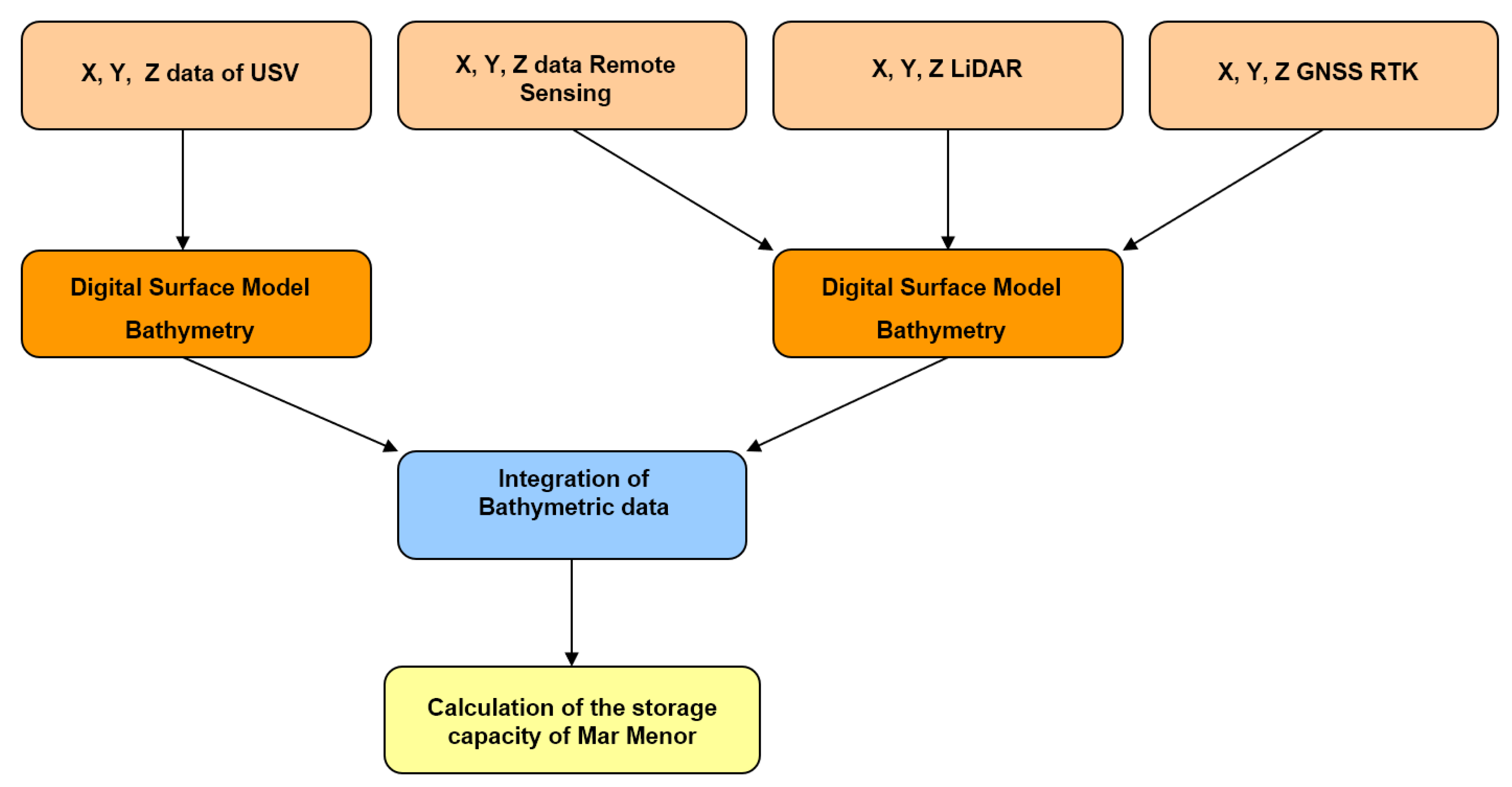
3.2.5. Integration of Altimetry Data for the Mar Menor Lagoon
The bathymetric datasets were integrated in an ArcGiS 10.7 geodatabase containing the LiDAR data of two years (2008 and 2016). Using all the data, a DEM was generated with a spatial resolution of 2 m, to perform the volume calculation for each isobath (m) and thus to compute the volume (m3) of the Mar Menor lagoon. The volume between each isobath was calculated, starting at the deepest level and finishing at the isobath corresponding to the maximum level of the Mar Menor lagoon. The final result corresponds to the height–volume relationship that is the current capacity curve. The applied methodology is represented in the flowchart in Figure 8.
The Digital Terrain Model (DTM) was derived by triangulation from the spatial resolutions of 1 m (Figure 9, Appendix A). Considering the vertex of the National Geodetic Network closest to each reservoir, the supporting points were taken with bi-frequency GPS. The datasets were processed with ArcGiS 10.7 (ESRI, Redlands, CA, USA) software. Subsequently, the points cloud with known X, Y, Z coordinates was calculated in the official terrestrial space reference system (ETRS89) and in the official vertical spatial reference system in Spain (EVRS89), based on the Earth Gravitational Model (EGM2008) of the National Geospatial-Intelligence Agency (NGA) EGM Development Team. Subsequently, a Triangular Irregular Network (TIN) mesh was generated using ArcGiS 10.7 (ESRI, Redlands, CA, USA) and this was used to calculate the volume of the Mar Menor lagoon.
4. Results
The results show that multispectral optical imagery with very high spatial (i.e., 0.5 m) and temporal (in this study, 22 images) resolution is suitable for the tracking of water-level fluctuations of the Mar Menor golas and shallows at a fine scale. The results are a function of the different steps of the project; these are summarized as follows:
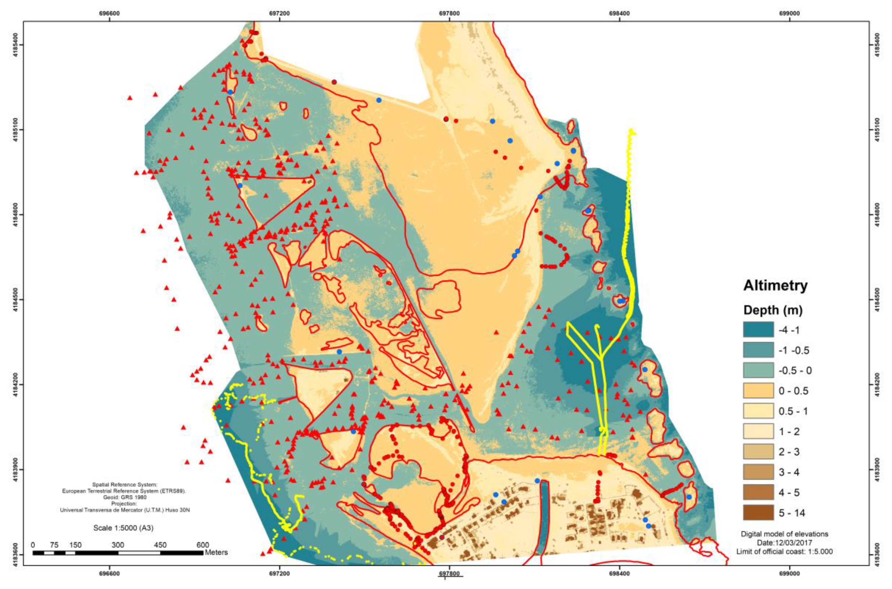
IMIDA06 USV has been developed by IPH and IMIDA and has provided a good bathymetry map (for 13 March 2017), with a spatial resolution of 50 cm and an error equal to ±3 cm (Figure 9).
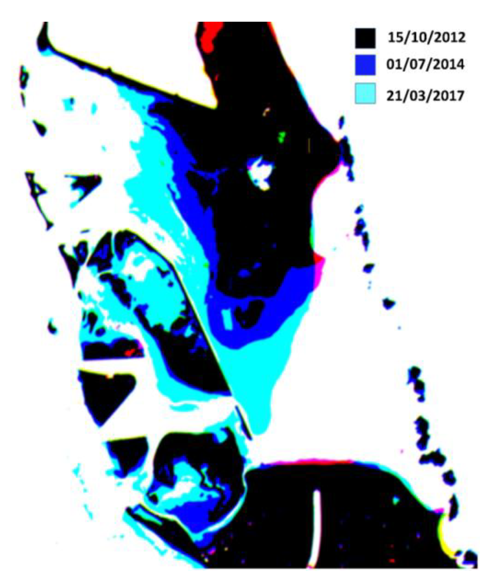
The NDWI values allow to evaluate the change of the water body and golas, as well as the annual movement of sediments and land area (Figure 10, Appendix A).
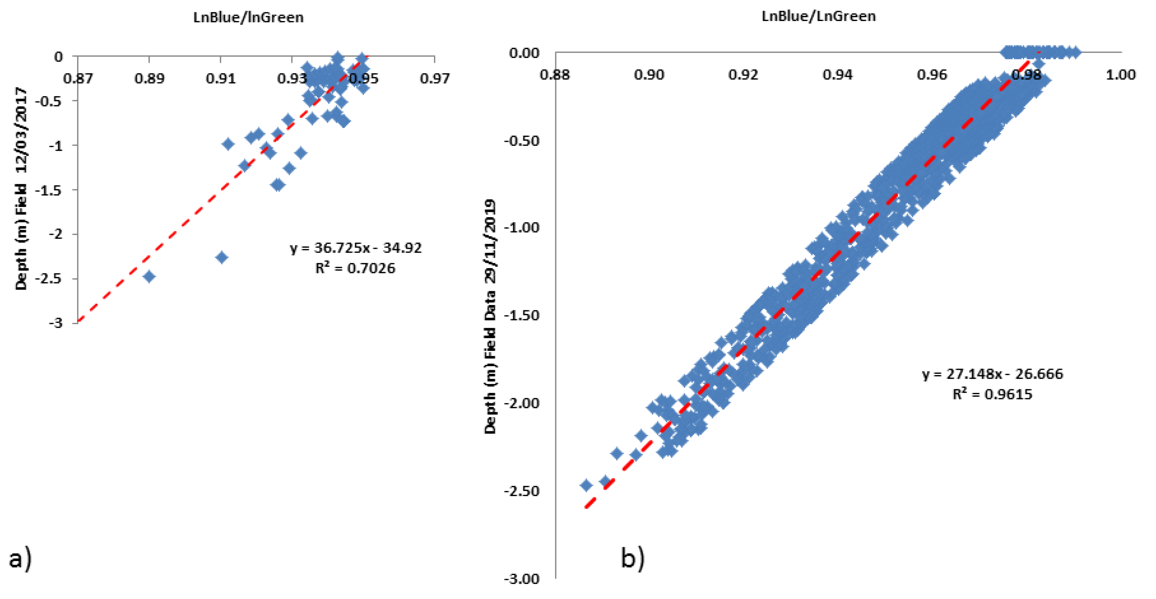
At the same time, the Water Depth Extraction Model [90] allows to obtain a bathymetric map from different satellite images and the parameters of this model (m and n). These parameters are not constant and depend on the water clarity (Figure 11).
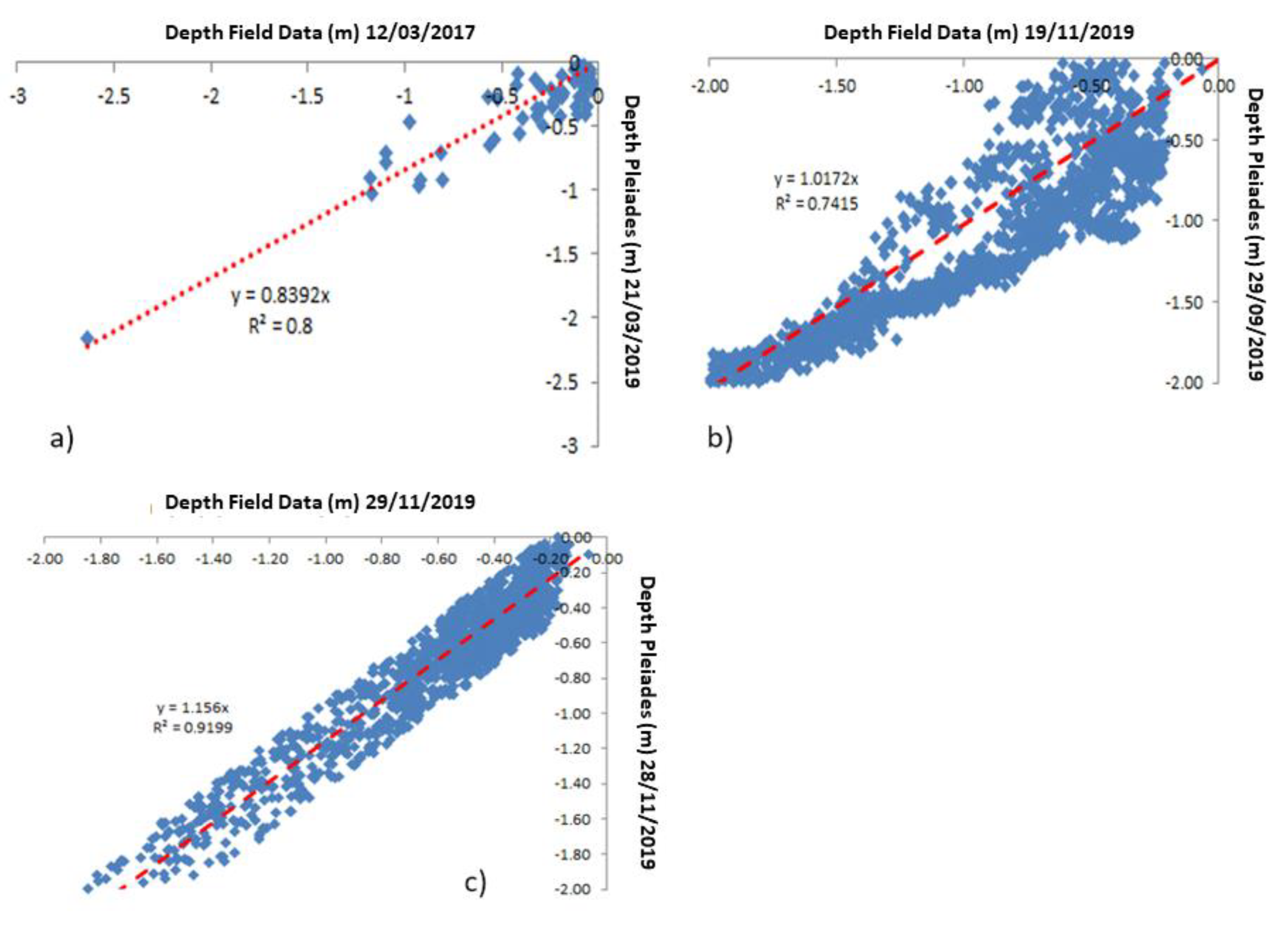
The relationship between both methods showed a good fit. On one hand, the slope of the regression is close to 1 (0.84 in the case of low transparency and 1.02 with clear waters), indicating the accuracy of the satellite image estimations and field data. The RMSE was analyzed at three different dates (Figure 12): one, five, and ten days of difference between the field data and the image. Firstly, for 2019, the RMSE2019 is 0.179 m. Secondly, the RMSE2017 is 0.186 m. Finally, in 2019, the image precedes the CoLs and the field data are subsequent to it; RMSE2019CoLs = 0.311 m. Besides, the slope of the line is reasonably close to 1: 0.92, 0.84, and 1.02. The RMSE values represent the accuracy of the measurements and dispersion of the data, while the slope is the true measure of accuracy.
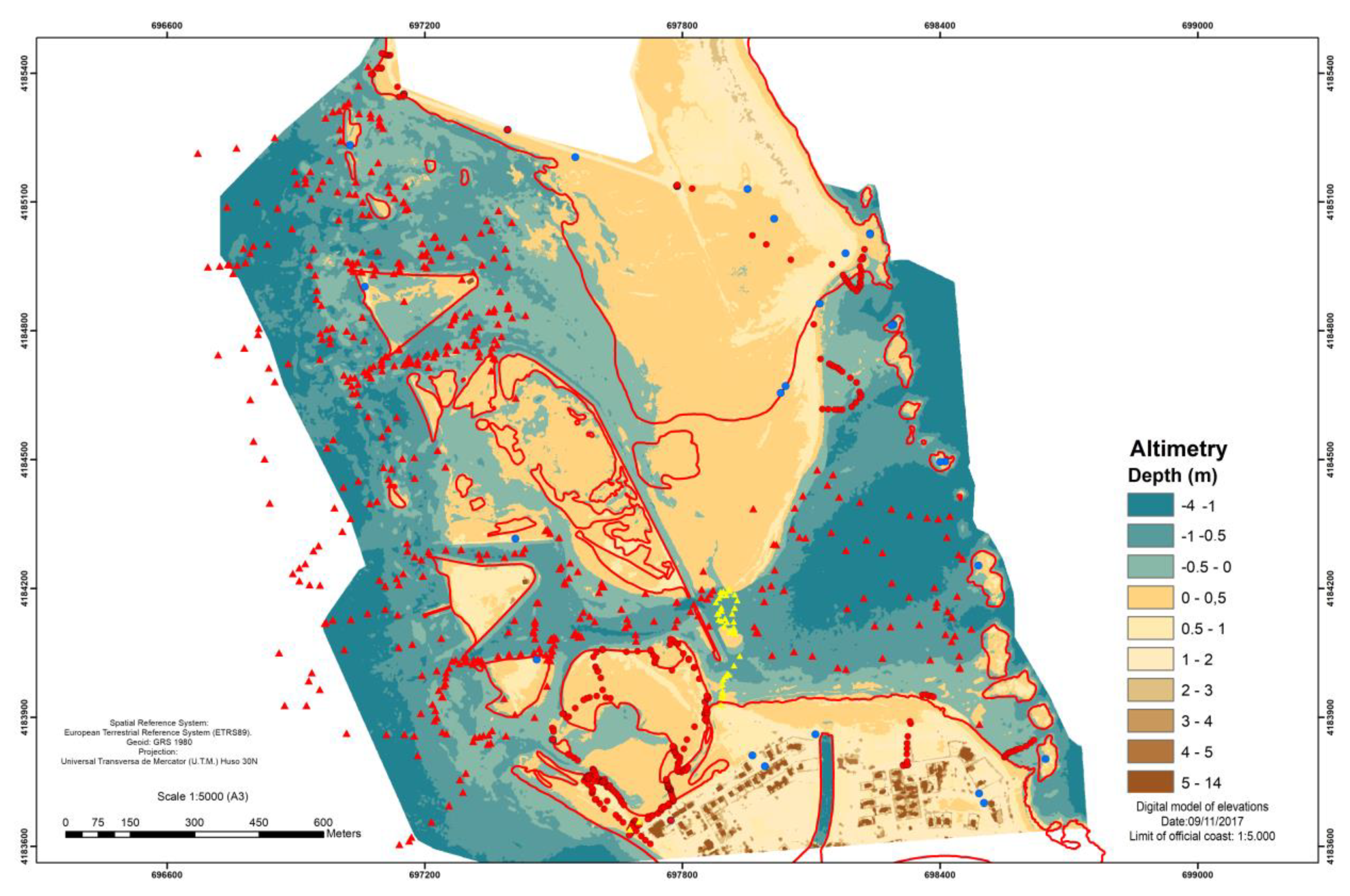
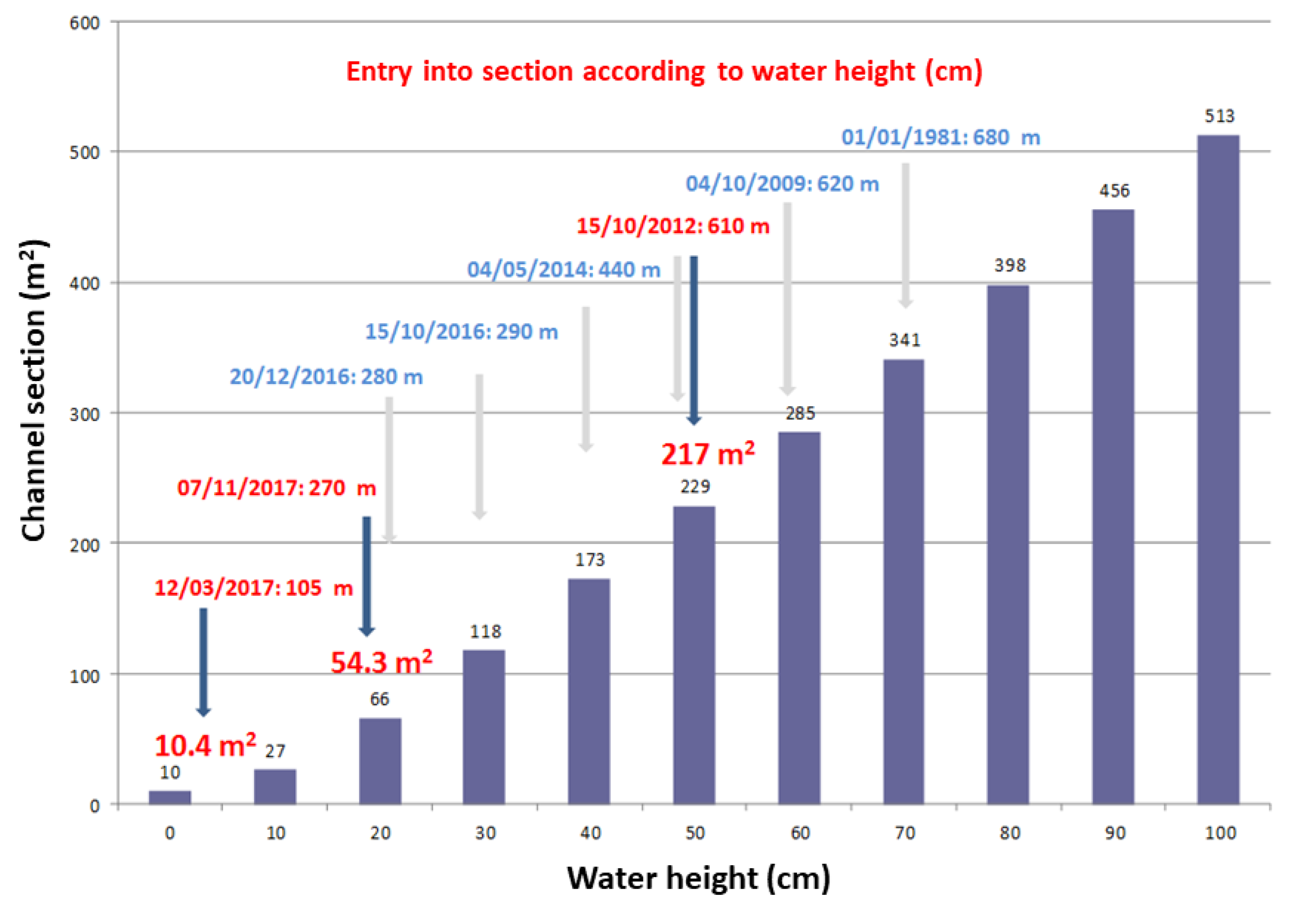
The bathymetric map obtained from the Pleaides satellite images of 11 November 2017 (Figure 13) allowed to calculate the exchange water between Mar Menor and the Mediterranean Sea. The exchanged volume increased the water level at Mar Menor due to the low atmospheric pressures registered from 15 October 2012 to 28 November 2019 (Figure 14).
The bathymetry, the barometric pressure, and the wind of the Mar Menor are responsible for the currents and therefore for the distribution of sediments in the lagoon. Therefore, an updated and high-resolution bathymetric characterization is especially important in order to know its evolution and its dynamics at different spatio-temporal scales. In addition, an accurate bathymetry is decisive to know the total volume of water in the lagoon and for hydrodynamic calculations, relevant to the determination of the water exchanges between Mar Menor and the Mediterranean Sea, through the three active golas. Mar Menor is a coastal lagoon with a high degree of hydrodynamic confinement and, as such, is the final recipient of all the transport processes that take place in the large (1350 km2) watershed of Campo de Cartagena. The soil uses in the coastal area has undergone significant transformations in the last decade, which have contributed to the acceleration of these transport processes and, consequently, the bottom of the lagoon have experienced an increasing accumulation of sediments (Figure 15) between 2008 and 2009 and between 2016 and 2017 (Table 4 and Table 5).
Mar Menor underwent a generalized silting up (an average of +18 cm) between 2008 and 2016, mainly the result of sediment contributions due to the very frequent extreme precipitation events [47]. Very intense rainfall events with a high return period occurred in the Campo of Cartagena in the last decade. As examples, the event of 27–28 September 2009 corresponded to a 200-year return period, where the CA12 rain gauge (located in La Palma) recorded 268 mm in 30 h. Then, during the event registered between 17 and 19 December 2016 in Campo of Cartagena (with a 500-year return period), the rainfall exceeded 50 mm in one hour in the Torre Pacheco (TP42) and San Javier (TP22) rain gauges [47]. Finally, the CoLs event named dana of 12–15 September 2019 generated maximum hourly rainfall intensities of 70.4 mm and 60.6 mm at the Torre Pacheco and Pozo Estrecho rain gauges, respectively. The maximum daily rainfall of 217.8 mm recorded by the Torre Pacheco rain gauge (12 September 2019 12:00 h to 13 September 2019 12:00 h) corresponded to a 500-year return period and generated severe flash floods in the Campo of Cartagena area. The estimations of return periods were based on [48] by applying the SQRT-ETmax cumulative distribution function.
5. Discussion
The deployment of an IMIDA06 USV is an example of how the free disposition of research findings can stimulate scientific advances, with the contribution of anyone, anywhere in the world. The images and their distribution are low-cost, which has allowed the development of new prototypes that, in turn, will be surpassed by novel work. Now it is necessary to take advantage of the developments from the recent years and make them useful to the community. In this sense, the IMIDA06 USV, as a source of field data, has allowed the development of a satellite image tracking system that is able to provide valuable data that helps solve environmental, social, and economic problems.
The Mar Menor lagoon and its area of influence is a complex and dynamic environmental, economic, and social system [94]; therefore, distinct types of information are necessary for its good management. The use of 3D numerical models represents a solution to obtain data and predict situations in the short term. However, model inputs condition the results and, therefore, special attention should be paid to their accuracy and precision; e.g., the initial conditionals (Xo, Yo, Zo) have to be precise enough. Remote sensing provides information on large coastal water bodies, such as the Mar Menor lagoon, besides providing good precision for Xo and Yo. However, knowing the depth, even in the shallowest waters, requires transparent waters that allow the sunlight to reach and be reflected by the bottom.
The initial idea was to use an unmanned aerial vehicle or unscrewed aerial vehicle (UAV), but in this area the use of a UAV is prohibited due to military activities. However, it is possible to use high spatial resolution satellite images to obtain a real-time bathymetry with an acceptable error that can be applied in different fields, such as scientific research, technology, and management.
At the same time, the idea was to select several places where very high spatial resolution bathymetric data could be obtained, using an aquatic drone, and then relate this data to the high spatial resolution images from satellites.
During this work, different water situations were induced by CoLs. This allowed producing distinct equations according to the transparency of the water, and a good adjustment with an acceptable RMSE was obtained. The methodology was improved by introducing a new step, since after calculating the relationship between LnBlue and LnGreen, the analysis of the ratio values is necessary for choosing the appropriate algorithm.
The changes in the depth of the lagoon depend mainly on the sediment loads mainly transported by runoff during flash-flood events, which deposit soil and other particles on the bottom. This contribution can reach 1863 t yr−1 [95]. Contributions from the Mediterranean or exchanges through the inlets have not been studied in depth, but there is evidence that they can be significant throughout the recent history of the Mar Menor lagoon, especially during extreme storm events [96]. Sedimentation rates have changed during the evolution of the Mar Menor lagoon linked to human uses in the drainage basin, and have increased with time, from 30 mm/century before the Middle Age to more than 30 cm/century in the 20th century, particularly due to deforestation and agricultural practices [97]. To the best of our knowledge, no work had been done that allowed to know the recent changes and the spatial variability of the sedimentation rates in the lagoon.
In the present work, the lowest RMSE value obtained was 0.179 m and increased over time; in 2017 it was 0.186 m and after the CoLs of 2019 there was a random movement and deposition of sand according to the RMSE value.
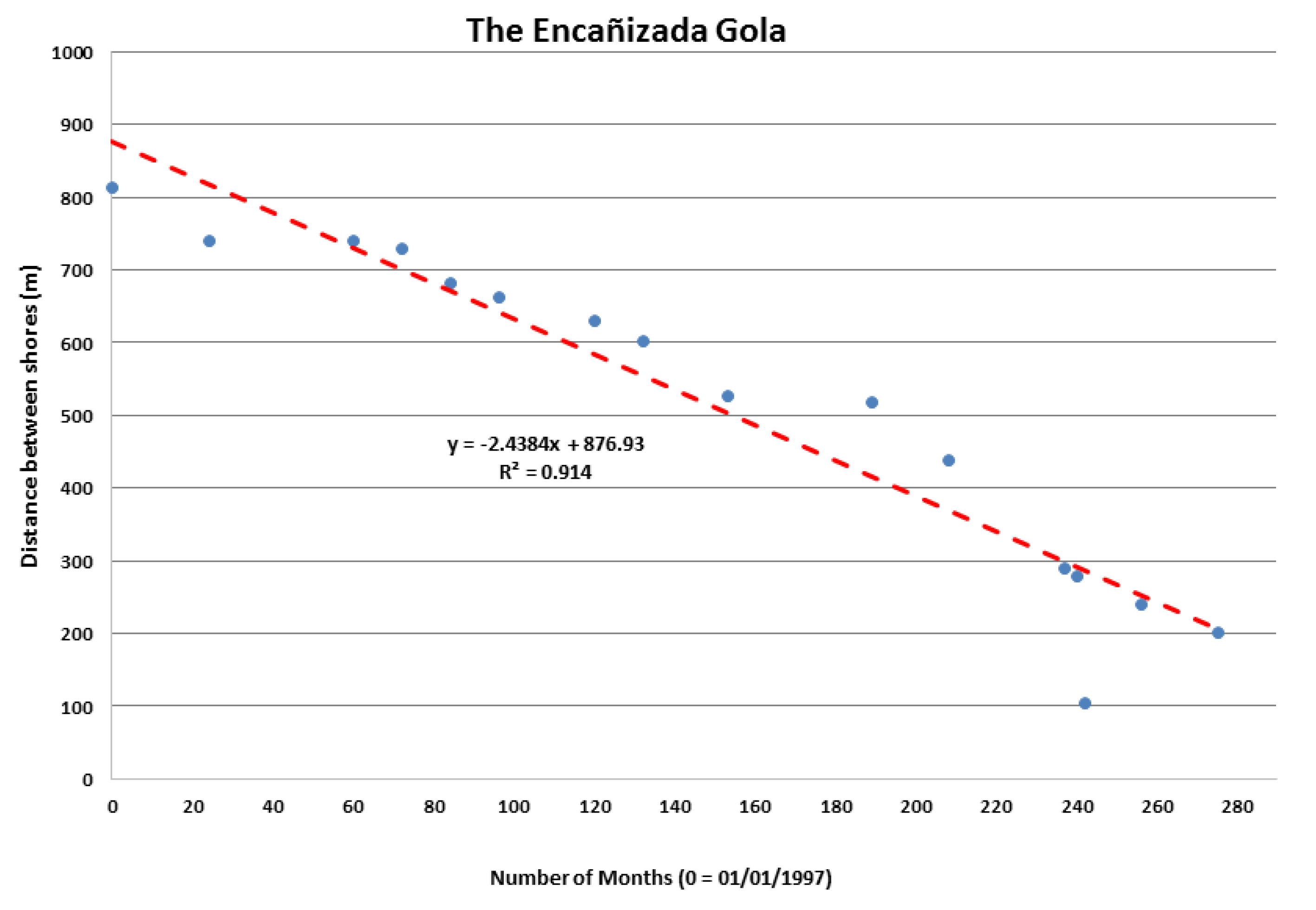
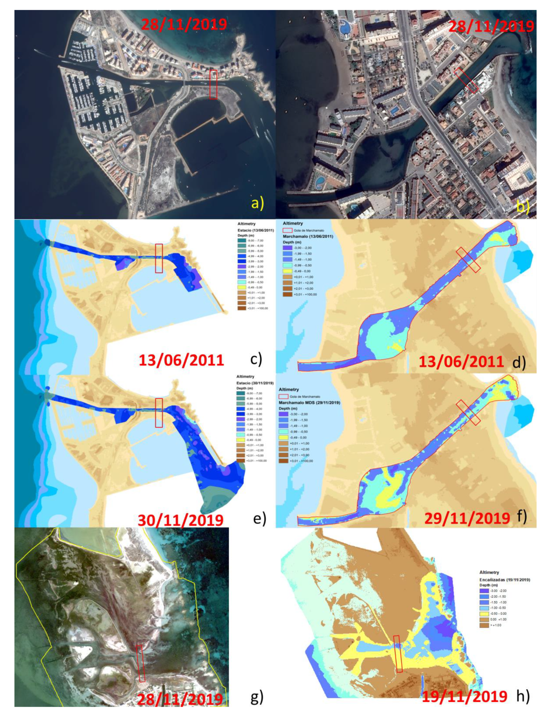
In the Encañizada gola the deposition of sand meant that the channel, through which water enters and leaves the Mar Menor lagoon, has gradually closed over time (Figure 16). In the Marchamalo and Estacio golas the deposition of sand meant that the channels were shallower compared to the last bathymetry carried out by the UPCT, in 2011 (Figure 17).
It was demonstrated that multispectral images are enough to obtain a precise bathymetry in shallow water. In this case, the shallow water is defined by the fact that the sunlight reaches the bottom of the lagoon. It was possible because, as shown in the bathymetric map, the maximum depth in the Mar Menor lagoon is 7 m; however, a depth of 4 m is presented in the photic zone, and this is the depth of the lagoon that it has been determined using optical sensors from different platforms: satellite, aircraft, or UAV.
The hyper-high spatial resolution of the sensor allows to obtain enough spatial detail, while the high resolution provides a temporal vision to observe details of the influence of the tides. Since the acquisition of the images is always at the same time and in the same place, the variation in the amount of water can only be due to movement of sand or movement of water.
The generated maps provide much information for the management of such a complicated area, but the most important thing is not only the information itself, but that it can be generated in quasi real time, allowing stakeholders to have accurate data in a short time for decision making. The depth model allows the use of images, obtained by aerial drones, of very high spatial resolution (18 cm) or the ones that the stakeholder prefers, since the resolution depends on the drone flight height; it can even reach 3 cm. As the gola is a small area, the stakeholder could have the bathymetric map a few hours after the flight. The low cost of obtaining spatial information from an area with great dynamism between water and land will allow the development of predictive models of soil movements and of increases or decreases in the amount of water in the gola. These models will provide the stakeholders enough information to be able to take decisions about the area with the aim of enhancing its conservation and the use of its resources. If the studies had been limited to the Encañizadas gola alone (Supplementary Materials S2), the sight of the importance of the other golas and the movement of water through them, between the Mediterranean Sea and the Mar Menor lagoon, would not have been known. Therefore, increasing knowledge of the movement of the sand in all the golas is fundamental for the area, in both economic and environmental terms (Figure A1 and Figure A3).
6. Conclusions
Once again, remote sensing was shown to be a tool, perhaps the most effective and cheapest one, for obtaining precise data. It may be used in 3D numerical models and in the management of the aquatic environment. It is necessary to remember that the Mar Menor lagoon is a dynamic ecosystem and the quantities of water and sand in each location within it are changing over time. Thus, although the bathymetric map generated throughout this work is the most up-to-date, it will be necessary to validate it from time to time due to the dynamic nature of the lagoon.
The results obtained show that the sedimentation processes occurring in the golas have produced a considerable reduction in their storage capacity, according the bathymetry. Although no significant changes have been detected in the current water renewal time in the lagoon compared to those estimated in the 1980s [25,27,83], the salinity has shown a tendency to approach the lower values of Mediterranean salinity rather than an increase [26]. It would be important to know how the observed changes can affect the capacity for water exchange between the Mar Menor lagoon and the Mediterranean Sea. In addition, climate change will negatively affect the frequency and intensity of natural hazards, such as extreme rainfall events in the area. Therefore, more frequent and severe flash flood events are expected for the contributing basins of the Mar Menor lagoon, which would affect their hydrodynamic [29] and sedimentation rates.
The bathymetries obtained from high-resolution satellite images, such as Pleiades, are demonstrated as very useful tools for complementing the bathymetries obtained with echo sounders in areas of shallow (<2 m) and clear water (Figure A2). Consequently, the precision of the calculation of the water volume of the Mar Menor lagoon has improved over time with the incorporation of new, much more precise technologies, such as interferometric echo sounders.
Supplementary Materials
These are available online at https://geoportal.imida.es/agua, (S1), together with a video on YouTube (S2): https://youtu.be/TdIUD8-K2Zw.
Author Contributions
The co-authors contributed in similar proportions to the work; the main author M.E. developed the concept and methodology and contributed to all sections of the work; J.A.D. and S.G.-G. contributed to the writing, review, and editing; J.F.A. contributed to the design of the experiments and the formal analysis; J.S. contributed to the formal analysis; Á.P.-R. contributed to the contextualization of the work in the framework of the hydrodynamic and ecological functioning of coastal lagoons and the evolution and the main changes in the geomorphology, hydrography and biological communities of the Mar Menor lagoon. All authors have read and agreed to the published version of the manuscript.
Funding
This research was co-funded (80%) by the European Regional Development Fund (ERDF), through grant number FEDER 14-20-25.
Acknowledgments
This work was done with the financial support of the research project FEDER 14-20-25, 80% co-funded by the European Regional Development Fund (ERDF). The authors are grateful to D. G. del Mar Menor, Department of Chemical & Environmental Engineering of UPCT, Instituto Español de Oceanografía (IEO) and the CTIN, Inntelia, and Airbus companies for their help in this experimentation.
Conflicts of Interest
The authors declare no conflict of interest.
Appendix A
The physical model used in this project is presented as follows:
R(0−,λ) = Rwater(0−,λ) + Rbottom(0−,λ).
The influence of the bottom is determined by a simple model, in which the bottom optical properties and the water optical properties are included [49,50]:
where Z is the depth and Kd the downwelling diffuse attenuation coefficient.
Rbottom(0−,λ) = [Rbottom(0−,λ) − Rwater(0−,λ)]exp(−2Zkd)
R−(z, λ) = R−w (λ) + [Rb(λ) − R−w (λ)] exp[−2Kd(λ)z]
[R−(z, λ) − R−w (λ)] = [Rb(λ) − R−w (λ)] exp[−2Kd(λ)z]
[1 − ] ~1; [1 − ] ~1 because the water is clear, thus R−w (λ) is very low [89]:
R−(z, λ) = Rb(λ) · exp[−2Kd(λ)z]
ln[R−(z, λ)] = ln [Rb(λ) exp[−2Kd(λ)z]
ln[R−(z, λ)] = ln [Rb(λ)] − 2Kd(λ)z
For the i band it is ln [R−(z, λi)] = ln [Rb(λi)] − 2Kd(λi)z
For the j band it is ln [R−(z, λj)] = ln [Rb(λj)] − 2Kd(λj)z
The ratio between ln [R−(z, λi)] and ln[R−(z, λj)] is
Kd(λi) ~ Kd(λj) ~ Kd because the water is clear [89]:
where m and n do not vary with depth (they are constant when the properties of the water column and the bottom are constant, too), but Ri (Green band) and Rj (Blue band) do vary.
Appendix B
Figure A1.
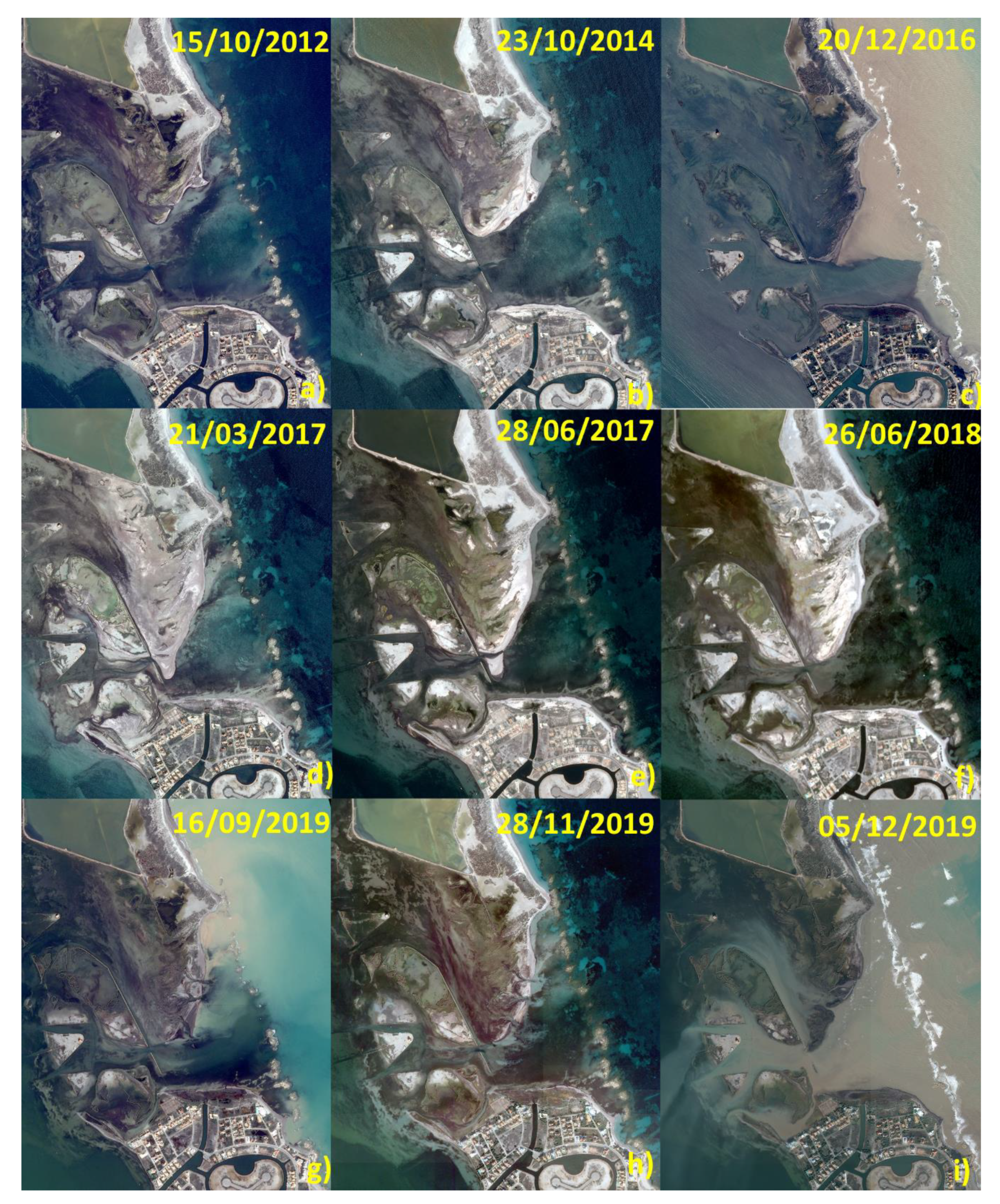
Pleiades images time series of the study: (a) First image available (15 October 2012); (b) The sediment accumulation process is evident; (c) During the first cut-off lows (CoLs); (d) Sediment accumulation process after the first CoLs; (e) Start of depth restoration; (f) Final of depth restoration; (g) During the second CoLs; (h) Sediment accumulation process after the second CoLs; (i) During the third CoLs (5 December 2019).
Figure A1.
Pleiades images time series of the study: (a) First image available (15 October 2012); (b) The sediment accumulation process is evident; (c) During the first cut-off lows (CoLs); (d) Sediment accumulation process after the first CoLs; (e) Start of depth restoration; (f) Final of depth restoration; (g) During the second CoLs; (h) Sediment accumulation process after the second CoLs; (i) During the third CoLs (5 December 2019).

Figure A2.
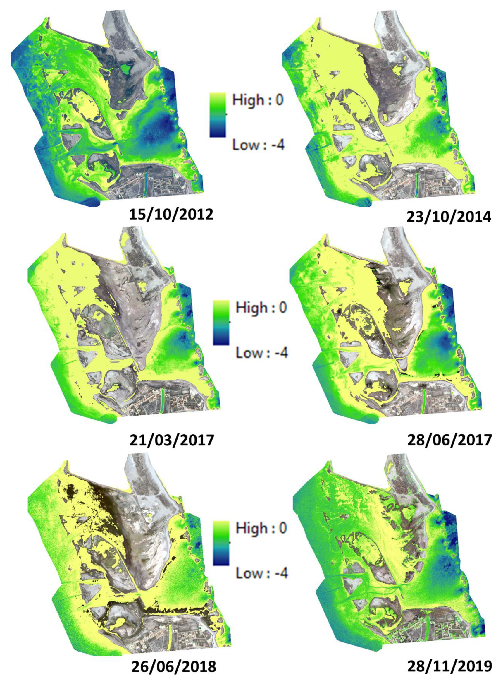
Bathymetry time series using Pleiades images between 15 October 2012 and 28 November 2019.
Figure A2.
Bathymetry time series using Pleiades images between 15 October 2012 and 28 November 2019.

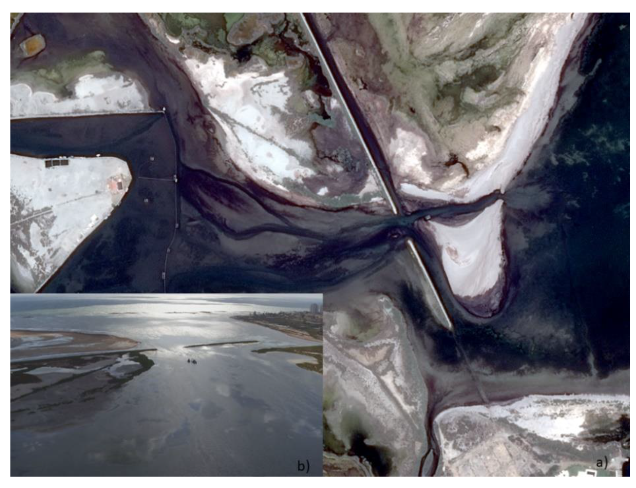
Figure A3.
Start of depth restoration in the Encañizada: (a) Pleiades image 28 June 2017; and (b) aerial image 15 August 2017, after the completion of maintenance work.
Figure A3.
Start of depth restoration in the Encañizada: (a) Pleiades image 28 June 2017; and (b) aerial image 15 August 2017, after the completion of maintenance work.

References
- De Pascalis, F.; Ghezzo, M.; Umgiesser, G.; De Serio, F.; Mossa, M. Use of Shyfem open source hydrodynamic model for time scales analysis in a semi-enclosed basin. In Proceedings of the 2016 IEEE Workshop on Environmental, Energy, and Structural Monitoring Systems (EESMS), Bari, Italy, 13–14 June 2016. [Google Scholar] [CrossRef]
- Wild-Allen, K.; Andrewartha, J. Connectivity between estuaries influences nutrient transport, cycling and water quality. Mar. Chem. 2016, 185, 12–26. [Google Scholar] [CrossRef]
- Yin, Y.; Karunarathna, H.; Reeve, D.E. Numerical modelling of hydrodynamic and morphodynamic response of a meso-tidal estuary inlet to the impacts of global climate variabilities. Mar. Geol. 2019, 407, 229–247. [Google Scholar] [CrossRef] [Green Version]
- Lesser, G.R.; Roelvink, J.A.; van Kester, J.; Stelling, G.S. Development and validation of a three-dimensional morphological model. Coastal Eng. 2004, 51, 883–915. [Google Scholar] [CrossRef]
- Lazure, P.; Garnier, V.; Dumas, F.; Herry, C.; Chiet, M. Development of a hydrodynamic model of the Bay of Biscay. Validation of hydrology. Cont. Shelf Res. 2009, 29, 985–997. [Google Scholar] [CrossRef] [Green Version]
- Sedigh, M.; Tomlinson, R.; Cartwright, N.; Etemad-Shahidi, A. Numerical modelling of the Gold Coast Seaway area hydrodynamics and littoral drift. Ocean Eng. 2016, 121, 47–61. [Google Scholar] [CrossRef]
- Gunn, K.; Stock-Williams, C. On validating numerical hydrodynamic models of complex tidal flow. Int. J. Mar. Energy 2013, 3, e82–e97. [Google Scholar] [CrossRef]
- Garneau, C.; Duchesne, S.; St-Hilaire, A. Comparison of modelling approaches to estimate trapping eficiency of sedimentation basins on peatlands used for peat extraction. Ecol. Eng. 2019, 133, 60–68. [Google Scholar] [CrossRef]
- De Pablo, H.; Sobrinho, J.; Garcia, M.; Campuzano, F.; Juliano, M.; Neves, R. Validation of the 3D-MOHID hydrodynamic model for the Tagus coastal area. Water 2019, 11, 1713. [Google Scholar] [CrossRef] [Green Version]
- Ma, G.; Shi, F.; Kirby, J.T. Shock-capturing non-hydrostatic model for fully dispersive surface wave processes. Ocean Modell. 2012, 43–44, 22–35. [Google Scholar] [CrossRef]
- Kirby, J.T.; Dalrymple, R.A. A parabolic equation for the combined refraction-diffraction of stokes waves by mildly varying topography. J. Fluid Mech. 1983, 136, 453–466. [Google Scholar] [CrossRef] [Green Version]
- Penven, P.; Marchesiello, P.; Debreu, L.; Lefevre, L. Software tools for pre- and post-processing of oceanic regional simulations. Environ. Modell. Softw. 2008, 23, 660–662. [Google Scholar] [CrossRef] [Green Version]
- Grifoll, M.; Del Campo, A.; Espino, M.; Mader, J.; González, M.; Borja, Á. Water renewal and risk assessment of water pollution in semi-enclosed domains: Application to Bilbao Harbour (Bay of Biscay). J. Mar. Syst. 2013, 109–110, S241–S251. [Google Scholar] [CrossRef]
- Guerreiro, M.; Fortunato, A.B.; Freire, P.; Rilo, A.; Taborda, R.; Freitas, M.C.; Andrade, C.; Silva, T.; Rodrigues, M.; Bertin, X.; et al. Evolution of the hydrodynamics of the Tagus estuary (Portugal) in the 21st century. J. Integr. Coast. Z. Manag. 2014, 15, 65–80. [Google Scholar] [CrossRef]
- Zhang, Y.; Baptista, A.M. SELFE: A semi-implicit Eulerian–Lagrangian finite-element model for cross-scale ocean circulation. Ocean Modell. 2008, 21, 71–96. [Google Scholar] [CrossRef]
- Zhang, Y.; Ye, F.; Stanev, E.V.; Grashorn, S. Seamless cross-scale modelling with SCHISM. Ocean Modell. 2016, 102, 64–81. [Google Scholar] [CrossRef] [Green Version]
- Ye, F.; Zhang, Y.; Friedrichs, M.; Wang, H.V.; Irby, I.; Shen, J.; Wang, Z. A 3D, cross-scale, baroclinic model with implicit vertical transport for the Upper Chesapeake Bay and its tributaries. Ocean Modell. 2016, 107, 82–96. [Google Scholar] [CrossRef]
- Umgiesser, G.; Ferrarin, C.; Cucco, A.; De Pascalis, F.; Bellafiore, D.; Ghezzo, M.; Bajo, M. Comparative hydrodynamics of 10 Mediterranean lagoons by means of numerical modeling. J. Geophys. Res. Oceans 2014, 119, 2212–2226. [Google Scholar] [CrossRef]
- Cucco, A.; Quattrocchi, G.; Olita, A.; Fazioli, L.; Ribotti, A.; Sinerchia, M.; Tedesco, C.; Sorgente, R. Hydrodynamic modelling of coastal seas: The role of tidal dynamics in the Messina Strait, Western Mediterranean Sea. Nat. Hazards Earth Syst. Sci. 2016, 16, 1553–1569. [Google Scholar] [CrossRef] [Green Version]
- Van Dongeren, A.; Svendsen, I. Absorbing-generating boundary condition for shallow water models. J. Waterw. Port Coast. 1997, 123, 303–313. [Google Scholar] [CrossRef]
- Booij, N.; Ris, R.; Holthuijsen, L.H. A third-generation wave model for coastal regions: 1. Model description and validation. J. Geophys. Res. 1999, 104, 7649–7666. [Google Scholar] [CrossRef] [Green Version]
- Gaeta, M.G.; Samaras, A.G.; Federico, I.; Archetti, R.; Maicu, F.; Lorenzetti, G. A coupled wave-3-D hydrodynamics model of the Taranto Sea (Italy): A multiple-nesting approach. Nat. Hazards Earth Syst. Sci. 2016, 16, 2071–2083. [Google Scholar] [CrossRef] [Green Version]
- Chubarenko, B.; Koutitonsky, V.G.; Neves, R.; Umgiesser, G. Modeling concepts. In Coastal Lagoons: Ecosystem Processes and Modeling for Sustainable Use and Development; Gönenc, I.E., Wolflin, J.P., Eds.; CRC Press: Boca Ratón, FL, USA, 2005; pp. 231–306. [Google Scholar]
- López-Castejón, F. Caracterización de la Hidrodinámica Del Mar Menor y Los Flujos de Intercambio Con El MEDITERRÁNEO Mediante Datos in Situ y Modelado Numérico. Ph.D. Thesis, Universidad Politécnica de Cartagena, Cartagena, Spain, 2017. [Google Scholar]
- Garcia-Oliva, M.; Perez-Ruzafa, A.; Umgiesser, G.; McKiver, W.; Ghezzo, M.; De Pascalis, F.; Marcos, C. Assessing the hydrodynamic response of the mar menor lagoon to dredging inlets interventions through numerical modelling. Water 2018, 10, 959. [Google Scholar] [CrossRef] [Green Version]
- García-Oliva, M.; Marcosa, C.; Umgiesserb, G.; McKiverb, W.; Ghezzo, M.; De Pascalisb, F.; Pérez-Ruzafa, A. Modelling the impact of dredging inlets on the salinity and temperature regimes in coastal lagoons. Ocean Coast. Manag. 2019, 180, 104913. [Google Scholar] [CrossRef]
- Ghezzo, M.; De Pascalis, F.; Umgiesser, G.; Zemlys, P.; Sigovini, M.; Marcos, C.; Pérez-Ruzafa, A. Connectivity in three European coastal lagoons. Estuaries Coasts 2015, 38, 1764–1781. [Google Scholar] [CrossRef]
- Pérez-Ruzafa, A.; Ghezzo, M.; De Pascalis, F.; Quispe, J.; Hernández-García, R.; Muñoz, I.; Vergara-Chen, C.; Umgiesser, G.; Marcos, C. Connectivity between coastal lagoons and sea: Reciprocal effects on assemblages’ structure and consequences for management. Estuar. Coast. Shelf Sci. 2019, 216, 171–186. [Google Scholar] [CrossRef]
- De Pascalis, F.; Pérez-Ruzafa, A.; Gilabert, J.; Marcos, C.; Umgiesser, G. Climate change response of the Mar Menor coastal lagoon (Spain) using a hydrodynamic finite element model. Estuar. Coast. Shelf Sci. 2012, 114, 118–129. [Google Scholar] [CrossRef]
- European Union. Directive 2007/60/EC of the European Parliament and of the Council of 23 October 2007 on the assessment and management of flood risks. Off. J. Eur. Parliam. 2007, 2455, 27–34. [Google Scholar]
- Ibarra, A.D. Análisis y Evolución de las Playas de la Región de Murcia (1956–2013). Ph.D. Thesis, Universidad de Murcia, Murcia, Spain, 2015. Available online: http://hdl.handle.net/10201/51348d (accessed on 13 December 2019).
- Lyard, F.; Genco, M.L. Optimization methods for bathymetry and open boundary conditions in a finite element model of ocean tides. J. Comput. Phys. 1994, 114, 234–256. [Google Scholar] [CrossRef]
- Chen, X. A cartesian method for fitting the bathymetry and tracking the dynamic position of the shoreline in a three-dimensional, hydrodynamic model. J. Comput. Phys. 2004, 200, 749–768. [Google Scholar] [CrossRef]
- Du Bois, P.B. Automatic calculation of bathymetry for coastal hydrodynamic models. Comput. Geosci. 2011, 37, 1303–1310. [Google Scholar] [CrossRef]
- Ardani, S.; Kaihatu, J.M. Optimization of bathymetry estimates for nearshore hydrodynamic models using bayesian methods. J. Waterw. Port Coast. 2018, 144, 04018024. [Google Scholar] [CrossRef]
- Ye, F.; Zhang, Y.J.; Wang, H.V.; Friedrichs, M.A.M.; Irby, I.D.; Alteljevich, E.; Valle-Levinson, A.; Wang, Z.; Huang, H.; Shen, J.; et al. A 3D unstructured-grid model for Chesapeake Bay: Importance of bathymetry. Ocean Modell. 2018, 127, 16–39. [Google Scholar] [CrossRef] [Green Version]
- Jo, Y.-H.; Sha, J.; Kwon, J.-I.; Jun, K.; Park, J. Mapping bathymetry based on waterlines observed from low altitude Helikite remote sensing platform. Acta Oceanol. Sin. 2015, 34, 110–116. [Google Scholar] [CrossRef]
- Chénier, R.; Faucher, M.-A.; Ahola, R. Satellite-derived bathymetry for improving Canadian hydrographic service charts. ISPRS Int. J. Geo Inf. 2018, 7, 306. [Google Scholar] [CrossRef] [Green Version]
- Legleiter, C.J.; Harrison, L.R. Remote sensing of river bathymetry: Evaluating a range of sensors, platforms, and algorithms on the upper Sacramento River, California, USA. Water Resour. Res. 2018, 55, 3. [Google Scholar] [CrossRef]
- Brêda, J.P.L.F.; Paiva, R.C.D.; Bravo, J.M.; Passaia, O.A.; Moreira, D.M. Assimilation of satellite altimetry data for effective river bathymetry. Water Resour. Res. 2019, 55, 9. [Google Scholar] [CrossRef]
- Sagawa, T.; Yamashita, Y.; Okumura, T.; Yamanokuchi, T. Satellite derived bathymetry using machine learning and multi-temporal satellite images. Remote Sens. 2019, 11, 1155. [Google Scholar] [CrossRef] [Green Version]
- Favre, A.; Hewitson, B.; Lennard, C.; Cerezo-Mota, R.; Tadross, M. Cut-off Lows in the South Africa region and their contribution to precipitation. Clim. Dyn. 2013, 41, 2331. [Google Scholar] [CrossRef]
- IEO. Estudio del Fondo Marino de la Laguna Costera del Mar Menor; IEO: Madrid, Spain, 2018. [Google Scholar]
- Erena, M.; Domínguez, J.A.; Aguado-Giménez, F.; Soria, J.; García-Galiano, S. Monitoring coastal lagoon water quality through remote sensing: The mar menor as a case study. Water 2019, 11, 1468. [Google Scholar] [CrossRef] [Green Version]
- Caballero, I.; Ruiz, J.; Navarro, G. Sentinel-2 satellites provide near-real time evaluation of catastrophic floods in the west mediterranean. Water 2019, 11, 2499. [Google Scholar] [CrossRef] [Green Version]
- Austin, R.W. The remote sensing of spectral radiance from below the ocean surface. In Optical Aspects of Oceanography; Jerlov, N.G., Steemann-Nielsen, E., Eds.; Academic Press: London, UK, 1974; pp. 317–344. [Google Scholar]
- Cánovas-García, F.; García-Galiano, S.; Alonso-Sarría, F. Assessment of satellite and radar quantitative precipitation estimates for real time monitoring of meteorological extremes over the Southeast of the Iberian Peninsula. Remote Sens. 2018, 10, 1023. [Google Scholar] [CrossRef] [Green Version]
- De Fomento, M. Dirección General de Carreteras. Máximas Lluvias Diarias en la España Peninsular; Ministerio de Fomento: Madrid, Spain, 1999. [Google Scholar]
- Kirk, J.T.O. Light and Photosynthesis in Aquatic Ecosystem, 1st ed.; Cambridge University Press: New York, NY, USA, 1994. [Google Scholar]
- Kutser, T. Quantitative detection of chlorophyll in cyanobacterial blooms by satellite remote sensing. Limnol. Oceanogr. 2004, 49, 2179–2189. [Google Scholar] [CrossRef]
- Philpot, W.D. Radiative transfer in stratified waters: A single scattering approximation for irradiance. Appl. Optics 1987, 26, 4123–4132. [Google Scholar] [CrossRef] [PubMed]
- Polcyn, F.C.; Brown, W.L.; Sattinger, I.J. The Measurement of Water Depth by Remote Sensing Techniques; Universidad de Michigan: Ann Arbor, MI, USA, 1970. [Google Scholar]
- Hasell, P.G. Michigan Experimental Multispectral Mapping System a Description of the M7 Airborne Sensor and ITS; NASA: Washington, DC, USA, 1974.
- NOAA. Hydrologic Optics. Vol. V. Properties. Colo Pacific Marine Environmental Lab. Honolulu; NOAA: Silver Spring, MD, USA, 1976. [Google Scholar]
- Lyzenga, D.R. Passive remote sensing techniques for mapping water depth and bottom features. Appl. Opt. 1978, 17, 379. [Google Scholar] [CrossRef] [PubMed]
- Lyzenga, D.R. Shallow-water bathymetry using combined lidar and passive multispectral scanner data. Int. J. Remote Sens. 1985, 6, 115–125. [Google Scholar] [CrossRef]
- Martitorena, S.; Morel, A.; Gentili, B. Diffuse reflectance of oceanic shallow waters: Influence of water depth and bottom albedo. Limnol. Oceanogr. 1994, 39, 1689–1703. [Google Scholar] [CrossRef]
- Bierwirth, P.N.; Lee, T.J.; Burne, R.V. Shallow seam floor reflectance and water depth derived by unmixing multispectral imagery. Photogramm. Eng. Remote Sens. 1993, 59, 331–338. [Google Scholar]
- Dierssen, H.M.; Zimmerman, R.C.; Leathers, R.A.; Downes, T.V.; Davis, C.O. Ocean color remote sensing of seagrass and bathymetry in the bahamas banks by high resolution airborne imagery. Limnol. Oceanogr. 2003, 48, 444–455. [Google Scholar] [CrossRef]
- Stumpf, R.P.; Holderied, K.; Sinclair, M. Determination of water depth with high-resolution satellite imagery over variable bottom types. Limnol. Oceanogr. 2003, 48, 547–556. [Google Scholar] [CrossRef]
- Olayinka, D.N.; Okolie, C.J. Bathymetric mapping of nigerian coastal waters from optical imagery. J. Eng. Res. Kuwait 2017, 22, 112–132. [Google Scholar]
- Setiawan, K.T.; Adawiah, S.W.; Marini, Y.; Winarso, G. Bathymetry data extraction analysis using Landsat 8 Data. Int. J. Remote Sens. 2016, 13, 79–86. [Google Scholar] [CrossRef] [Green Version]
- Vanderstraete, T.; Goossens, R.; Ghabour, T.K. Can ASTER-Data Be Used for Bathymetric Mapping of Coral Reefs in the Red Sea Using Digital Photogrammetry, 2nd ed.; Workshop EARSeL Special Interest Group on Remote Sensing for Developing Countries, 18-20 September; Gunter, M., Matthias, B., Eds.; University Bonn: Bonn, Germany, 2003; pp. 212–218. [Google Scholar]
- Liang, J.; Zhang, J.; Ma, Y.; Zhang, C.Y. Derivation of bathymetry from high-resolution optical satellite imagery and usv sounding data. Mar. Geod. 2017, 40, 466–479. [Google Scholar] [CrossRef]
- Liu, S.; Gao, Y.; Zheng, W.; Li, X. Performance of two neural network models in bathymetry. Remote Sens. Lett. 2015, 6, 321–330. [Google Scholar] [CrossRef]
- Hernandez, W.J.; Armstrong, R.A. Deriving bathymetry from multispectral remote sensing data. J. Mar. Sci. Eng. 2016, 4, 8. [Google Scholar] [CrossRef]
- Mohamed, H.; Negm, A.; Zahran, M.; Saavedra, O.C. Bathymetry determination from high resolution satellite imagery using ensemble learning algorithms in shallow lakes: Case study el-burullus lake. Int. J. Environ. Sci. Dev. 2016, 7, 296–301. [Google Scholar] [CrossRef] [Green Version]
- Simon, R.N.; Tormos, T.; Danis, P.A. Very high spatial resolution optical and radar imagery in tracking water level fluctuations of a small inland reservoir. Int. J. App. Earth Obs. 2016, 38, 36–39. [Google Scholar] [CrossRef]
- Pérez-Ruzafa, A.; Gilabert, J.; Bel-Lan, A.; Moreno, V.; Gutierrez, J.M. New approach to chlorophyll a determination in shallow coastal waters by remote sensing. Sci. Mar. 1996, 60, 19–27. [Google Scholar]
- Yunus, A.P.; Dou, J.; Song, X.; Avtar, R. Improved bathymetric mapping of coastal and lake environments using Sentinel-2 and Landsat-8 images. Sensors 2019, 19, 2788. [Google Scholar] [CrossRef] [Green Version]
- Cahalanea, C.; Mageeb, A.; Monteysc, X.; Casalb, G.; Hanafind, J.; Harrise, A. Comparison of Landsat 8, RapidEye and Pleiades products for improving empirical predictions of satellite-derived bathymetry. Remote Sens. Environ. 2019, 233, 111414. [Google Scholar] [CrossRef]
- Flener, C. Estimating deep water radiance in shallow water: Adapting optical bathymetry modelling to shallow river environments. Boreal Environ. Res. 2013, 18, 488–502. [Google Scholar]
- Edwards, A.J. Applications of Satellite and Airborne Image Date to Coastal Management. Coastal region and Small Island, papers 4; UNESCO: Paris, France, 1999; p. 185. [Google Scholar]
- Committee on Earth Observing Satellites (CEOS). Feasibility Study for an Aquatic Ecosystem Earth Observing System. 2018. Available online: http://ceos.org/document_management/Publications/Feasibility-Study-for-an-Aquatic-Ecosystem-EOS-v.2-hi-res_05April2018.pdf (accessed on 12 December 2019).
- Jawak, S.D.; Vadlamani, S.S.; Luis, A.J. A synoptic review on deriving bathymetry information using remote sensing technologies: Models, methods and comparisons. Adv. Space Res. 2015, 4, 147–162. [Google Scholar] [CrossRef] [Green Version]
- Ferrandiz, C. La encañizada de Calnegre en la manga del mar menor y su formación en el siglo XVIII. Murgetana 1976, 45, 87–101. [Google Scholar]
- Del Río, V.D. Estudio Ecológico del Mar Menor. Geología, (Proyecto nº 1005 Medio Marino); IEO: Madrid, Spain, 1990. [Google Scholar]
- Lillo, M.J. Geomorfología del mar menor. Pap. Dep. Geogr. 1981, 8, 9–48. [Google Scholar]
- Serra, J. Mar Menor (Spain). EUROSION Case Study, Institut de Ciència i Tecnologia Ambientals; Universitat Autónoma de Barcelona: Bellaterra, Spain, 2013. [Google Scholar]
- Pérez-Ruzafa, A.; Mompeán, M.C.; Marcos, C. Hydrographic, geomorphologic and fish assemblage relationships in coastal lagoons. Hydrobiologia 2007, 577, 107–125. [Google Scholar] [CrossRef]
- Pérez-Ruzafa, A.; Marcos, C. Fisheries in coastal lagoons: An assumed but poorly researched aspect of the ecology and functioning of coastal lagoons. Estuar. Coast. Shelf Sci. 2012, 110, 15–31. [Google Scholar] [CrossRef]
- Pérez-Ruzafa, A.; Pérez-Ruzafa, I.M.; Newton, A.; Marcos, C. Chapter 15—Coastal lagoons: Environmental variability, ecosystem complexity, and goods and services uniformity. In Coasts and Estuaries: The Future; Wolanski, E., Day, J., Elliott, M., Ramachandran, R., Eds.; Elsevier: Amsterdam, The Netherlands, 2019; pp. 253–276. [Google Scholar]
- Pérez-Ruzafa, A. Estudio Ecológico y Bionómico de Los Poblamientos Bentónicos Del Mar Menor (Murcia, SE de España). Ph.D. Thesis, Universidad de Murcia, Murcia, Spain, 1989. [Google Scholar]
- Mėžinė, J.; Ferrarin, C.; Vaičiūtė, D.; Idzelytė, R.; Zemlys, P.; Umgiesser, G. Sediment transport mechanisms in a lagoon with high river discharge and sediment loading. Water 2019, 11, 1970. [Google Scholar] [CrossRef] [Green Version]
- Manley, J.E. High Fidelity Hydrographic Surveys Using and Autonomous Surface Craft; Massachusetts Institute of Technology: Cambridge, MA, USA, 1998. [Google Scholar]
- Manley, J.E.; Marsh, A.; Cornforth, W.; Wiseman, C. Evolution of the autonomous surface craft Autocrat. In Proceedings of the IEEE Conference and Exhibition on Oceans 2000 MTS, IEEE 2000, Providence, RI, USA, 11–14 September 2000; Volume 1, pp. 403–408. [Google Scholar]
- Brown, H.C.; Kim, A.; Eustice, R.M. An overview of autonomous underwater vehicle research and testbed at PeRL. Mar. Technol. Soc. J. 2009, 43, 33–47. [Google Scholar] [CrossRef]
- Erena, M.; Atenza, J.F.; García-Galiano, S.; Domínguez, J.A.; Bernabé, J.M. Use of drones for the topo-bathymetric monitoring of the reservoirs of the Segura river basin. Water 2019, 11, 445. [Google Scholar] [CrossRef] [Green Version]
- Domínguez Gómez, J.A.; Chuvieco Salinero, E.; Sastre Merlín, A. Monitoring transparency in inland water bodies using multispectral images. Int. J. Remote Sens. 2009, 30, 1567–1586. [Google Scholar] [CrossRef]
- Lia, J.; Knappa, D.; Schillb, S.; Roelfsemac, C.; Phinnc, S.; Silmand, M.; Mascaroe, J.; Asnera, G. Adaptive bathymetry estimation for shallow coastal waters using Planet Dove satellites. Remote Sens. Environ. 2019, 232, 111302. [Google Scholar] [CrossRef]
- Bernstein, L.; Adler-Golden, S.; Sundberg, R.; Levine, R.; Perkins, T.; Berk, A.; Ratkowski, A.; Felde, G.; Hoke, M. A new method for atmospheric correction and aerosol optical property retrieval for vis-swir multi- and hyperspectral imaging sensors: Quac (quick atmospheric correction). In Proceedings of the IEEE International Geoscience and Remote Sensing, Symposium, Seoul, Korea, 25–29 July 2005; Volume 5, pp. 3549–3552. [Google Scholar]
- Vanhellemont, Q.; Ruddick, K. ACOLITE for SENTINEL-2: Aquatic applications of MSI imagery. In Proceedings of the ESA Living Planet Symposium, Prague, Czech Republic, 9–13 May 2016. ESA Special Publication SP-740. [Google Scholar]
- McFeeters, S.K. The use of the normalized difference water index (NDWI) in the delineation of open water features. Int. J. Remote Sens. 1996, 17, 1425–1432. [Google Scholar] [CrossRef]
- Más, J. El Mar Menor. Relaciones, Diferencias y Afinidades Entre la Laguna Costera y el Mar Mediterráneo Adyacente; IEO: Madrid, Spain, 2006. [Google Scholar]
- García-Pintado, J.; Martínez-Mena, M.; Barberá, G.; Albaladejo, J.; Castillo, V. Anthropogenic nutrient sources and loads from a Mediterranean catchment into a coastal lagoon: Mar Menor, Spain. Sci. Total Environ. 2007, 37, 220–239. [Google Scholar] [CrossRef] [PubMed]
- Dezileau, L.; Perez-Ruzafa, A.; Blanchemanche, P.; Degeai, J.P.; Raji, O.; Martinez, P.; Marcos, C.; Von Grafenstein, U. Extreme storms during the last 6500 years from lagoonal sedimentary archives in the Mar Menor (SE Spain). Clim. Past 2016, 12, 1389–1400. [Google Scholar] [CrossRef] [Green Version]
- Pérez-Ruzafa, A.; Marcos, C.; Pérez-Ruzafa, I.; Ros, J.D. Evolución de las características ambientales y de los poblamientos del Mar Menor (Murcia, SE España). An. Biol. 1987, 12, 53–65. [Google Scholar]
Figure 1.
Study area in the Mar Menor lagoon. (a) Sentinel 3 image of the ESA, (b) Sentinel 2 image of the Mar Menor on 1 January 2019, and Pleiades 1A images on 28 November 2019 of the (c) Encañizadas, (d) Estacio, and (e) Marchamalo channels.
Figure 1.
Study area in the Mar Menor lagoon. (a) Sentinel 3 image of the ESA, (b) Sentinel 2 image of the Mar Menor on 1 January 2019, and Pleiades 1A images on 28 November 2019 of the (c) Encañizadas, (d) Estacio, and (e) Marchamalo channels.

Figure 2.
The topo-bathymetric work (a) CN Los Alcázares from a Pleiades image 20 December 2016; (b) IMIDA06 USV; (c) USV data collection software; and (d) Bathymetric points recorded on 30 January 2018.
Figure 2.
The topo-bathymetric work (a) CN Los Alcázares from a Pleiades image 20 December 2016; (b) IMIDA06 USV; (c) USV data collection software; and (d) Bathymetric points recorded on 30 January 2018.

Figure 3.
The five data collection areas where the Unmanned Surface Vehicle (USV) was used to provide data for calibrations of the algorithms designed to obtain bathymetries with Pleiades satellite images: CN Los Alcazares; CN Los Urrutias; Gola Marchamalo; Gola Estacio; and Gola Encañizadas.
Figure 3.
The five data collection areas where the Unmanned Surface Vehicle (USV) was used to provide data for calibrations of the algorithms designed to obtain bathymetries with Pleiades satellite images: CN Los Alcazares; CN Los Urrutias; Gola Marchamalo; Gola Estacio; and Gola Encañizadas.

Figure 4.
Spectral resolution of the Pleiades sensors (http://www.gstdubai.com/satelliteimagery/pleiades-1a.html).
Figure 4.
Spectral resolution of the Pleiades sensors (http://www.gstdubai.com/satelliteimagery/pleiades-1a.html).

Figure 5.
LiDAR data (2008) around the Mar Menor lagoon and MAGRAMA bathymetry in 2008.

Figure 6.
LiDAR data (2016) around the Mar Menor lagoon and IEO bathymetry [14] in 2016 (no data for a depth <−3 m, blue line).
Figure 6.
LiDAR data (2016) around the Mar Menor lagoon and IEO bathymetry [14] in 2016 (no data for a depth <−3 m, blue line).

Figure 7.
Workflow diagram with Pleiades images.

Figure 8.
Flowchart showing the integration of the LiDAR and bathymetric data of Mar Menor.

Figure 9.
Water depth estimated on 13 March 2017, using an USV, Pleiades, and ground data (red and blue points correspond to GPS data, while yellow points correspond to USV data). The red line corresponds to the coast in 1999.
Figure 9.
Water depth estimated on 13 March 2017, using an USV, Pleiades, and ground data (red and blue points correspond to GPS data, while yellow points correspond to USV data). The red line corresponds to the coast in 1999.

Figure 10.
Map showing the differences among the dates 15 October 2012, 23 May 2014, and 21 March 2017. It was produced using Pleiades images of the Encañizada channel.
Figure 10.
Map showing the differences among the dates 15 October 2012, 23 May 2014, and 21 March 2017. It was produced using Pleiades images of the Encañizada channel.

Figure 11.
Water Depth Extraction Model for two different water quality conditions: (a) 13 March 2017, less water transparency, and (b) 29 November 2019, more water transparency.
Figure 11.
Water Depth Extraction Model for two different water quality conditions: (a) 13 March 2017, less water transparency, and (b) 29 November 2019, more water transparency.

Figure 12.
Relationships between field and image data at three different dates: (a) 21 March 2017; (b) 19 November 2019; and (c) 29 November 2019.
Figure 12.
Relationships between field and image data at three different dates: (a) 21 March 2017; (b) 19 November 2019; and (c) 29 November 2019.

Figure 13.
Water depth determined using the USV and the Pleiades images of 11 November 2017, as well as ground data (red and blue points correspond to GPS data, while yellow points to USV data). The red line corresponds to the coast in 1999.
Figure 13.
Water depth determined using the USV and the Pleiades images of 11 November 2017, as well as ground data (red and blue points correspond to GPS data, while yellow points to USV data). The red line corresponds to the coast in 1999.

Figure 14.
Water exchange section (m2) in the Gola de las Encañizadas on different dates (values in red and blue) and for different water levels (m−2) induced by low atmospheric pressures (values in black).
Figure 14.
Water exchange section (m2) in the Gola de las Encañizadas on different dates (values in red and blue) and for different water levels (m−2) induced by low atmospheric pressures (values in black).

Figure 15.
Bathymetric evolution of Mar Menor between 2008 and 2009 and between 2016 and 2017.

Figure 16.
The monitoring of the deposition of sediment in the Encañizada (1997–2019).

Figure 17.
The monitoring of the sediment deposit: (a,c,e) El Estacio channel; (b,d,f) Marchamalo channel; and (g,h) Encañizada channel. The yellow areas correspond to depths less than 0.5 m. The rectangle red represents the zone of comparison between the bathymetries in the channels.
Figure 17.
The monitoring of the sediment deposit: (a,c,e) El Estacio channel; (b,d,f) Marchamalo channel; and (g,h) Encañizada channel. The yellow areas correspond to depths less than 0.5 m. The rectangle red represents the zone of comparison between the bathymetries in the channels.


Table 1.
Dates and characteristics of the field data used in the study of the channels.
| Organization | GPS | Photogrammetry | Sensor | MDS (m) | Date |
|---|---|---|---|---|---|
| IHM (MM) | Single probe | 1967 | |||
| IGN (out MM) | 0.5 p/m2 | Leica (ALS50) | 2 | 4/10/2009 | |
| MAGRAMA (MM) | 40 p/m2 | Seabat 8124 (200 kHz) | 1 | 4/10/2009 | |
| UPCT (En.) | Leica (TPS400) | ADCP (500 kHz) | 1 | 5/08/2010 | |
| UPCT (Ma.) | Leica (TPS400) | River Surveyor M9 | 1 | 19/08/2011 | |
| UPCT (Es.) | Leica (TPS400) | River Surveyor M9 | 1 | 19/08/2011 | |
| IEO (En.) | Garmin (GPS72) | 30 p/m2 | Hondex (PS-7) | 2 | 15/05/2014 |
| IGN (out MM) | 0.5 p/m2 | Leica (ALS50) | 2 | 4/10/2016 | |
| IEO (MM) | Trimble (SPS 751) | GeoSwath (500 kHz) | 1 | 13/06/2017 | |
| IMIDA (En.) | Leica (1200) | Airmar (50 kHz) | 1 | 12/03/2017 | |
| IMIDA (En.) | Leica (1200) | Airmar (50 kHz) | 1 | 7/11/2017 | |
| IMIDA (En) | Leica (1200) | Airmar (50 kHz) | 1 | 24/04/2018 | |
| IMIDA (En.) | Leica (1200) | ECT400S (450 kHz) | 1 | 19/11/2019 | |
| IMIDA (Ma.) | Leica (1200) | ECT400S (450 kHz) | 1 | 29/11/2019 | |
| IMIDA (Es.) | Leica (1200) | ECT400S (450 kHz) | 1 | 30/11/2019 |
Table 2.
Dates and characteristics of the images used to track the shallow water (<3 m).
| Satellite | Sensor | PAN | VIS | IRC | Res (m) | Date |
|---|---|---|---|---|---|---|
| Pleiades 1A | HiRi | 1 | 3 | 1 | 0.5/2 | 15/10/2012 |
| Pleiades 1A | HiRi | 1 | 3 | 1 | 0.5/2 | 1/07/2014 |
| Pleiades 1B | HiRi | 1 | 3 | 1 | 0.5/2 | 23/05/2014 |
| Pleiades 1A | HiRi | 1 | 3 | 1 | 0.5/2 | 12/10/2015 |
| Pleiades 1A | HiRi | 1 | 3 | 1 | 0.5/2 | 1/07/2016 |
| Pleiades 1A | HiRi | 1 | 3 | 1 | 0.5/2 | 15/10/2016 |
| Pleiades 1A | HiRi | 1 | 3 | 1 | 0.5/2 | 20/12/2016 |
| Pleiades 1B | HiRi | 1 | 3 | 1 | 0.5/2 | 21/03/2017 |
| Pleiades 1B | HiRi | 1 | 3 | 1 | 0.5/2 | 28/06/2017 |
| Pleiades 1A | HiRi | 1 | 3 | 1 | 0.5/2 | 9/11/2017 |
| Pleiades 1A | HiRi | 1 | 3 | 1 | 0.5/2 | 5/12/2017 |
| Pleiades 1B | HiRi | 1 | 3 | 1 | 0.5/2 | 15/04/2018 |
| Pleiades 1B | HiRi | 1 | 3 | 1 | 0.5/2 | 29/04/2018 |
| Pleiades 1B | HiRi | 1 | 3 | 1 | 0.5/2 | 18/05/2018 |
| Pleiades 1A | HiRi | 1 | 3 | 1 | 0.5/2 | 29/11/2018 |
| Pleiades 1A | HiRi | 1 | 3 | 1 | 0.5/2 | 4/09/2019 |
| Pleiades 1A | HiRi | 1 | 3 | 1 | 0.5/2 | 16/09/2019 |
| Pleiades 1B | HiRi | 1 | 3 | 1 | 0.5/2 | 24/09/2019 |
| Pleiades 1B | HiRi | 1 | 3 | 1 | 0.5/2 | 29/09/2019 |
| Pleiades 1A | HiRi | 1 | 3 | 1 | 0.5/2 | 28/11/2019 |
| Pleiades 1A | HiRi | 1 | 3 | 1 | 0.5/2 | 5/12/2019 |
Table 3.
Specifications of the Unmanned Surface Vehicle (USV) components (IMIDA06).
| Part Name | Model/Number | Specifications | Function |
|---|---|---|---|
| Boat hull | Inntelia | Fiberglass | Navigation |
| Motors | BlueRobotics | Thruster-R1 | Main actuator |
| Propellers | T-200 | 350 W | Propulsion |
| Microcontroller | Pixhawk 3.2.1 | Open hardware | Navigation control |
| Battery (LiPo) | Tattu 22.2V | 15C 4500 mAh | Power supply |
| Radio receiver | UHF | 1 W (−30 dB) | Radio command |
| GNSS | EMLID | NMEA 0183 | GPS antenna |
| Graupner | 12 ch. PCM | 2.4 GHz | Control station |
| Software | APM | 3.2 | Mission planner |
| Echo sounder | Airmar/DST 700 | 50/200 kHz | Echo sounder |
Table 4.
Estimates of the surface areas and volumes per isobath, as well as the total cumulative volume of Mar Menor in 2008 and 2016.
Table 4.
Estimates of the surface areas and volumes per isobath, as well as the total cumulative volume of Mar Menor in 2008 and 2016.
| Isobath (m) | Surface Area (2008) (km2) | Vol (2008) (109 m3) | VT (2008) (109 m3) | Surface Area (2016) (km2) | Vol (2016) (109 m3) | VT (2016) (109 m3) |
|---|---|---|---|---|---|---|
| −7 | 9.720 | 0.003 | 0.003 | 0.393 | 0.000 | 0.000 |
| −6 | 39.312 | 0.021 | 0.024 | 45.498 | 0.018 | 0.018 |
| −5 | 82.262 | 0.064 | 0.088 | 84.780 | 0.068 | 0.086 |
| −4 | 99.449 | 0.092 | 0.180 | 102.564 | 0.095 | 0.181 |
| −3 | 110.138 | 0.105 | 0.285 | 112.532 | 0.108 | 0.288 |
| −2 | 117.504 | 0.114 | 0.399 | 119.432 | 0.116 | 0.404 |
| −1 | 126.044 | 0.121 | 0.521 | 126.335 | 0.123 | 0.527 |
| 0 | 138.127 | 0.132 | 0.653 | 135.202 | 0.130 | 0.657 |
VT = Total cumulative volume; Vol = Volume per isobath.
Table 5.
The volume of the Mar Menor and characteristics of the exchange channels.
| Organization/Bibliography | Area | Volume (109 m3) | Section (m2) | Depth (m) | Date |
|---|---|---|---|---|---|
| UMU [49] | Mar Menor | 0.580 | 1980–1988 | ||
| IEO [58] | Mar Menor | 0.580 | - | - | 1988 |
| UPCT [4] | Mar Menor | 0.725 | - | - | 2011 |
| UMU/ISMAR [7] | Mar Menor | 0.600 | 2009–2010 | ||
| IMIDA | Mar Menor | 0.653 | - | - | 2009 |
| IMIDA | Mar Menor | 0.657 | - | - | 2016 |
| IEO [14] | Mar Menor | 0.654 | - | - | 2017 |
| UPCT [4] | Encañizada | - | 207 | −0.40 | 5/08/2010 |
| UPCT [4] | Estacio | - | 208 | −5.20 | 13/06/2011 |
| UPCT [4] | Marchamalo | - | 21 | −1.12 | 13/06/2011 |
| IEO | Encañizada | - | 145 | −0.35 | 15/05/2014 |
| IMIDA | Encañizada | - | 11 | −0.10 | 21/03/2017 |
| IMIDA | Encañizada | - | 54 | −0.20 | 28/11/2018 |
| IMIDA | Encañizada | - | 120 | −0.44 | 19/11/2019 |
| IMIDA | Marchamalo | - | 21 | −0.78 | 29/11/2019 |
| IMIDA | Estacio | - | 204 | −5.10 | 30/11/2019 |
© 2020 by the authors. Licensee MDPI, Basel, Switzerland. This article is an open access article distributed under the terms and conditions of the Creative Commons Attribution (CC BY) license (http://creativecommons.org/licenses/by/4.0/).
Share and Cite
MDPI and ACS Style
Erena, M.; Domínguez, J.A.; Atenza, J.F.; García-Galiano, S.; Soria, J.; Pérez-Ruzafa, Á. Bathymetry Time Series Using High Spatial Resolution Satellite Images. Water 2020, 12, 531. https://doi.org/10.3390/w12020531
AMA Style
Erena M, Domínguez JA, Atenza JF, García-Galiano S, Soria J, Pérez-Ruzafa Á. Bathymetry Time Series Using High Spatial Resolution Satellite Images. Water. 2020; 12(2):531. https://doi.org/10.3390/w12020531
Chicago/Turabian StyleErena, Manuel, José A. Domínguez, Joaquín F. Atenza, Sandra García-Galiano, Juan Soria, and Ángel Pérez-Ruzafa. 2020. "Bathymetry Time Series Using High Spatial Resolution Satellite Images" Water 12, no. 2: 531. https://doi.org/10.3390/w12020531
Note that from the first issue of 2016, this journal uses article numbers instead of page numbers. See further details here.