Mathematical Model of Small-Volume Air Vessel Based on Real Gas Equation

Abstract

The gas characteristics of an air vessel is one of the key parameters that determines the protective effect on water hammer pressure. Because of the limitation of the ideal gas state equation applied for a small-volume vessel, the Van der Waals (VDW) equation and Redlich–Kwong (R–K) equation are proposed to numerically simulate the pressure oscillation. The R–K polytropic equation is derived under the assumption that the volume occupied by the air molecules themselves could be ignored. The effects of cohesion pressure under real gas equations are analyzed by using the method of characteristics under different vessel diameters. The results show that cohesion pressure has a significant effect on the small volume vessel. During the first phase of the transient period, the minimum pressure and water depth calculated by a real gas model are obviously lower than that calculated by an ideal gas model. Because VDW cohesion pressure has a stronger influence on the air vessel pressure compared to R–K air cohesion pressure, the amplitude of head oscillation in the vessel calculated by the R–K equation becomes larger. The numerical results of real gas equations can provide a higher safe-depth margin of the water depth required in the small-volume vessel, resulting in the safe operation of the practical pumping pipeline system.

1. Introduction

Pump failure can result in severe water hammer events, especially in long-distance water-supply pumping systems [1]. To avoid the adverse effect of a water hammer, an air vessel, which is also known as air chamber or volumetric tank, is usually introduced to the pipeline systems as the protection measure. Therefore, the accurate mathematic model of an air vessel is necessary and important for water hammer simulation during pump failure [2,3,4].

As an airtight high-pressure container, the air vessel is usually installed in the pipeline adjacent to the pump outlet for the purpose of negative pressure prevention after pump failure [5,6,7,8]. Wood [9] carried out analytical and experimental investigations, and the results showed that air vessels could attenuate the pressure surges well along the pipeline. Sun et al. [10] and Yang [11] pointed out the hydraulic transients after the pump failure can be effectively controlled by reflecting the pressure wave and reducing head oscillation in the air vessel. The protective effect greatly depends on the characteristics of expansion and contraction of gas. That is, the performance of the air vessel on pressure wave reflection and pressure surge control is affected by the characteristics of gas in the vessel.

The polytropic equation of an ideal gas is extensively used for describing the gas characteristics in the vessel. However, the thermodynamic process of the gas in a confined container is not satisfied with the reversible polytropic process of ideal gas because of the dissipation effect between gas and water surface or gas and wall during the transient process in pipeline system. Thus, the assumption of the ideal gas is actually not consistent with the gas characteristics in practical pipeline system. When analyzing the impact of a water hammer on pressure variations in pipelines protected by an air vessel, the measured pressure values were compared with numerical results from the ideal gas assumption [12]. A deviation between the measured and calculated pressures existed, which validated the above inference well. In addition, the effects of related vessel parameters, such as the initial air volume, wave speed, orifice diameter and the polytropic exponent, to minimize a water hammer were investigated by both the numerical calculations and the experiments [13]. However, the effect of the real gas characteristics was not taken into account.

Furthermore, the experimental investigations conducted by Jones et al. [14] confirmed that the gas approximately followed the law of the ideal gas state equation only under low temperature. Under high pressure, however, any gas would not completely follow the reversible polytropic relation. The higher pressure is in air vessel, the greater deviations between the numerical results from ideal equation and measured values will be. As for the air vessel of a small volume, the pressure fluctuation of the air vessel is usually huge during the transient process, undergoing high pressure. Therefore, the equation of state of the ideal gas was not suitable for the gas characteristics in the small-volume air vessel. Thus, the equations of state of the real gas (Van der Waals (VDW) equation and Redlich–Kwong (R–K) equation) was proposed in this paper.

The VDW equation and R–K equation are the primary equations of state of gas describing the real gas characteristics. The above equations of state of a real gas were presented by Moran et al. [15] and the range of applications was discussed as well. It is well known that the VDW equation is an equation of state for the air composed of particles that have a non-zero volume and a pairwise attractive and repulsive inter-particle force. The equation was based on a modification of the ideal gas law [16], and considered the nonzero size of molecules and the attraction between them [17], which was approximated to the behavior of a real gas. Van der Waals [18] obtained the equations of state based on cohesion pressure terms. It is found that, the equation is also qualitatively reasonable for both the liquid state and gaseous state for lower temperatures. Furthermore, many phenomena, including supercooling and superheating, were correctly predicted with the assistance of the Van der Waals equation [19]. Redlich and Kwong [20] improved the accuracy of the VDW equation by introducing temperature into the cohesion pressure term, which has been widely used in computer procedures for predicting real gas behavior in recent years. The R–K equation was generally conceded to be one of the best generalized two parameter equations of state available. In addition, it was remarkably compact, and attractive for inclusion in large-scale process design computer programs which required efficient data calculation procedures to be effective [21].

Gas characteristics have great influence on the polytropic exponent of a thermodynamic process. The most common solution to such a process was the isothermal (n = 1) or isentropic assumption (n = 1.4) [22]. An average value of 1.2 may be used in design calculations [23,24,25], whereas the value is short of theoretical support. Fast transients, field observations and experiments showed that n was approximately 1.4 in closed air pockets, and the thermodynamic behavior was close to adiabatic with zero heat transfer [26,27,28,29,30]. However, when calculating closed surge tank behavior for slow transients, Zhou et al. [31] showed that heat transfer had a significant effect on the thermodynamics of the system and was, therefore, not properly represented by the polytrophic equation. In long-distance water-supply transmission pipelines, the vessel oscillation period was caused by an instantaneous check valve closure. Consequently, it was reasonable to assume the heat exchange was sufficient, and the polytropic exponent value was 1.0 [32]. Based on the comprehensive analysis above, the thermodynamic process of the air vessel can be considered as an isothermal process, and corresponding polytropic exponent value is 1.0 for a long-distance water-supply pumping system.

The key innovative features of this paper are as follows: (1) derivation of the R–K gas polytropic equation of the air vessel; (2) calculation and analysis of the air vessel model calculated by the ideal gas equation, VDW gas equation and R–K gas equation; (3) comparison of the air vessel model under different vessel diameters.

2. Equation of State of Gas

2.1. Equation of State of Ideal Gas

The polytropic equation of the ideal gas [25] is given below:

$$P_{\mathrm{Ideal}}{V_{\mathrm{Ideal}}}^{n_{\mathrm{Ideal}}}=C_1$$

(1)

$$n_{\mathrm{Ideal}}=1-\frac{R}{C-C_V}=\frac{C-C_P}{C-C_V}$$

(2)

where $P_{\mathrm{Ideal}}$ is the absolute pressure of the ideal gas, Pa, which is equal to the surface pressure plus the atmospheric pressure; $V_{\mathrm{Ideal}}$ is the volume of the ideal gas, m³; C₁ is the constant indicating the specific heat capacity. $n_{\mathrm{Ideal}}$ is the polytropic exponent of ideal gas; R is the individual gas constant. For air, R = 0.2867 KJ/(kg·K); C_P is specific heat at constant pressure, kJ/(kg·K); C_V is specific heat at constant volume, kJ/(kg·K); C is specific heat of mole, kJ/(kg·K). For air in the condition of 298.15 K, 100 kPa, C_P = 1.004 kJ/(kg·K), C_V = 0.717 kJ/(kg·K).

2.2. Equation of State of Van der Waals (VDW) Gas

For m moles of gas, Jin [33] shows the gas polytropic equation of VDW:

$$P_2{V}_{\mathrm{VDW}}^{n_{\mathrm{VDW}}}=C_2$$

(3)

$$P_2=P_{\mathrm{VDW}}+\frac{m^2{a}_{\mathrm{VDW}}}{V_2^2}$$

(4)

$$V_{\mathrm{VDW}}=V_2-m{b}_{\mathrm{VDW}}$$

(5)

$$n_{\mathrm{VDW}}=1-\frac{R}{C-C_V}$$

(6)

where $P_{\mathrm{VDW}}$ is the absolute pressure of the VDW gas, Pa; $V_{\mathrm{VDW}}$ is the effective volume in the VDW approximation, diminished due to the finite size of the molecules, that is, $V_{\mathrm{VDW}}$ is the actual volume of the VDW gas, m³; $a_{\mathrm{VDW}}$ is the pure component parameter of the VDW equation; $a_{\mathrm{VDW}}/V_2^2$ is called “cohesion pressure”, which takes the attractive (electrical (induced dipole-induced dipole) interaction in nature between gas molecules into account; $b_{\mathrm{VDW}}$ is the co-volume of the gas molecules; T is the absolute temperature of gas, K, $n_{\mathrm{VDW}}$ is the polytropic exponent of the VDW gas; C₂ is a constant. $a_{\mathrm{VDW}}$ and $b_{\mathrm{VDW}}$ are calculated by Equations (A1) and (A2) from Appendix A.1. For air, the values are $161.4744{\mathrm{m}}^6\times {\mathrm{Pa}/\mathrm{kg}}^2$, $1.2552\times {10}^{-3}{\mathrm{m}}^3/\mathrm{kg}$, respectively.

2.3. Equation of State of Redlich–Kwong (R–K) Gas

For m moles of gas, R–K equation [21] is described as:

$$\left(P_{\mathrm{RK}}+\frac{m^2{a}_{\mathrm{RK}}}{T^{0.5}{V}_3(V_3+m{b}_{\mathrm{RK}})}\right)\left(V_3-m{b}_{\mathrm{RK}}\right)=mRT$$

(7)

$$P_3=P_{\mathrm{RK}}+\frac{m^2{a}_{\mathrm{RK}}}{T^{0.5}{V}_3(V_3+m{b}_{\mathrm{RK}})}$$

(8)

$$V_{\mathrm{RK}}=V_3-m{b}_{\mathrm{RK}}$$

(9)

giving

$$P_3{V}_{\mathrm{RK}}=mRT$$

(10)

where $P_{\mathrm{RK}}$ is the absolute pressure of the RK gas, Pa; $V_{\mathrm{RK}}$ is the actual volume of the RK gas, m³; $a_{\mathrm{RK}}$ is the pure component parameters of cohesion pressure term; $b_{\mathrm{RK}}$ is the co-volume of the gas molecules. $a_{\mathrm{RK}}$ and $b_{\mathrm{RK}}$ are calculated by Equations (A3) and (A4) from Appendix A.1. For air, the values are $1883.6076{\mathrm{m}}^6\times \mathrm{Pa}\times {\mathrm{K}}^{0.5}{/\mathrm{kg}}^2$, 0.873 × 10⁻³ m³/kg, respectively.

The variation of internal energy of the system [34] can be expressed as:

$$\mathrm{d}U=m{C}_V\mathrm{d}T+\left[T{\left(\frac{\partial P_{RK}}{\partial T}\right)}_V-P_{RK}\right]\mathrm{d}{V}_3=m{C}_V\mathrm{d}T+1.5\frac{m^2{a}_{\mathrm{RK}}}{T^{0.5}{V}_3(V_3+m{b}_{\mathrm{RK}})}\mathrm{d}{V}_3$$

(11)

where dU is the small variation of internal energy.

According to the first law of thermodynamics, this gives:

$$\mathrm{d}Q=\mathrm{d}U+\mathrm{d}W$$

(12)

$$\mathrm{d}Q=C\mathrm{d}T$$

(13)

$$\mathrm{d}W=P_{\mathrm{RK}}\mathrm{d}{V}_3$$

(14)

where dQ is heat exchange between the internal and external system; dW is net work exchanged between the internal and external system.

By substituting Equations (11), (13) and (14) into Equation (12), this yields:

$$mC\mathrm{d}T=\mathrm{m}{C}_V\mathrm{d}T+1.5\frac{m^2{a}_{\mathrm{RK}}}{T^{0.5}{V}_3(V_3+m{b}_{\mathrm{RK}})}\mathrm{d}{V}_3+P_{RK}\mathrm{d}{V}_3$$

(15)

By substituting Equations (7) and (10) into Equation (15), this yields:

$$\left(1.5\frac{mRT}{V_{\mathrm{RK}}}-0.5P_{\mathrm{RK}}\right)\mathrm{d}{V}_3+m\left(C_V-C\right)\mathrm{d}T=0$$

(16)

in which $\mathrm{d}{V}_{\mathrm{RK}}=\mathrm{d}\left(V_3-m{b}_{\mathrm{RK}}\right)=\mathrm{d}{V}_3$. Then Equation (16) becomes:

$$1.5\frac{\mathrm{d}{V}_{\mathrm{RK}}}{V_{\mathrm{RK}}}-0.5\frac{P_{\mathrm{RK}}}{mRT}\mathrm{d}{V}_{\mathrm{RK}}+\frac{C_V-C}{R}\frac{\mathrm{d}T}{T}=0$$

(17)

The bulk volume of air molecules themselves is negligible compared with the air volume in the vessel ($V_3>>m{b}_{\mathrm{RK}}$). That is, the volume occupied by the air molecules themselves could be ignored, so an approximate treatment (V_RK ≈ V₃) is made.

By substituting Equations (7) and (10) and V_RK ≈ V₃ into Equation (17), this gives:

$$\frac{\mathrm{d}{V}_{\mathrm{RK}}}{V_{\mathrm{RK}}}+\frac{0.5m{a}_{\mathrm{RK}}}{R{T}^{1.5}{V}_{\mathrm{RK}}^2}\mathrm{d}{V}_{\mathrm{RK}}+\frac{C_V-C}{R}\frac{\mathrm{d}T}{T}=0$$

(18)

Since $R{T}^{1.5}{V}_{\mathrm{RK}}^2>>0.5m{a}_{RK}$, Equation (18) can be simplified as:

$$\frac{\mathrm{d}{V}_{\mathrm{RK}}}{V_{\mathrm{RK}}}+\frac{C_V-C}{R}\frac{\mathrm{d}T}{T}=0$$

(19)

According to Appendix A.2, Equation (19) can be rewritten as:

$$P_3{V}_{\mathrm{RK}}^{n_{\mathrm{RK}}}=C_3$$

(20)

$$n_{\mathrm{RK}}=1-\frac{R}{C-C_V}$$

(21)

where C₃ is a constant. Equation (21) is a simplified R–K gas polytropic equation under the assumption of the bulk volume of air molecules themselves could be negligible. $n_{\mathrm{RK}}$ is the R–K gas polytropic exponent. According to Equations (2), (6) and (21), the polytropic exponents of VDW and for the given approximation of RK do not differ from the ideal gas case.

3. Mathematical Model of Air Vessel

An air vessel is a container filled with compressed gas and water. In order to eliminate the positive surge and negative surge in the vessel, a connecting pipe is installed at the junction of the air vessel and the pipeline. The mathematic model of the air vessel is established, as shown in Figure 1. The following equations describe the head and flow equations at the junction of the air vessel and the pipeline [25].

The characteristic equations for sections U and D can be expressed as:

$$\mathrm{C}+:H_B=C_P-B_P\cdot Q_U$$

(22)

$$\mathrm{C}-:H_B=C_M+B_M\cdot Q_D$$

(23)

where $H_B$ is the hydraulic grade at junction P, m; $C_P$, $B_P$, $C_M$ and $B_M$ = constants in MOC (method of characteristic equations); U is the subscript which denotes the left boundary point of the air vessel; D is the subscript which denotes the right boundary point of the air vessel; $Q_U$ is the discharge into junction P, m³; $Q_D$ is the discharge out of junction P, m³.

The continuity equation at the junction P can be written as:

$$Q_S=Q_U-Q_D$$

(24)

where $Q_S$ is the discharge through the connecting pipe either in positive or negative direction, m³.

In the air vessel, water follows the relation:

$$\frac{d{H}_S}{dt}=\frac{Q_S}{A_S}$$

(25)

where $H_S$ is the water level of air vessel, m; Z is the water depth, m; $A_S$ is the cross-sectional area of air vessel, m²; t is the time, s.

In the vessel, the air follows the following polytropic relation:

$$P_i{V}_i{}^{n_j}=C_i$$

(26)

where i = 1, 2 and 3; P_i is the pressure of air, Pa, represent ideal, VDW and RK air, respectively; V_i is the actual (effective) volume of air, m³; n_j is the polytropic exponent; C_i is a constant.

If the elasticity of water and vessel wall is not considered, the air head and water level in the vessel are as follows:

$$\frac{P_j}{\rho g}=H_B-\sigma \frac{Q_S\left|Q_S\right|}{2g{A}_0^2}-H_S+\overline{H}$$

(27)

where P_j is the absolute pressure of air, Pa, represent ideal, VDW and RK air, respectively, under the condition of ideal gas model, P_i = P_j; ρ is density, for water, ρ = 1000 kg/m³; g is gravitational acceleration, 9.8 m/s²; $\overline{H}$ is atmospheric pressure head, m; σ is resistance coefficient of the connecting pipe; A₀ is the cross-sectional area of connecting pipe, m².

Considering Δt is very small according to the calculation of a water hammer, in which Δt is the time difference, according to Appendix A.3, Equation (27) can be rewritten as:

$$\frac{P_j}{\rho \mathrm{g}}=H_B-\frac{\sigma }{2g{A}_0^2}{Q}_S\left|Q_{S0}\right|-\left[H_{S0}+0.5\Delta t\frac{\left(Q_S+Q_{S0}\right)}{A_S}\right]+\overline{H}$$

(28)

where Q_S0 and Z₀ are the known discharge and water level at the time of t–Δt, respectively.

By substituting Equations (22)–(24) into Equation (28), this gives:

$$\frac{P_j}{\rho \mathrm{g}}=\overline{H}-\gamma \left[\left(\frac{C_P}{B_P}+\frac{C_M}{B_M}\right)-Q_S\right]/\left(\frac{1}{B_P}+\frac{1}{B_M}\right)-\gamma \left[H_{S0}+\frac{0.5\Delta t}{A_S}{Q}_{S0}+\left(\frac{0.5\Delta t}{A_S}+\frac{\sigma \left|Q_{S0}\right|}{2g{A}_0^2}\right)Q_S\right]$$

(29)

By substituting Equation (26) into Equation (28), the absolute pressure P_j ($P_{\mathrm{Ideal}}$, $P_{\mathrm{VDW}}$ and $P_{\mathrm{RK}}$) can be solved by the Newton–Raphson iteration method. Then, the other transient variables can be obtained.

4. Case Study

Figure 2 shows a long-distance water supply system equipped with an air vessel. The total length of the pipeline is 23.40 km, and the discharge is 0.35 m³/s. The water levels of suction sump and outlet sump of the pumping station are 1666.50 m and 1881.65 m, respectively. The air vessel temperature is 283.15 K. Three ASP-2B-21-200-580 pumps are installed in parallel, with one pump being backup unit. And the head of pump is 245.55 m. A check valve is mounted at the outlet of pump for each pumping subline.

Since the air vessel is installed nearest to the pump discharge, the fluid in the air vessel will enter the pipeline rapidly after the pump failure. In order to reduce the size of the air vessel, the check valve mounted at the outlet of pump is set to be in one-period closing mode with instantaneous closing time of 1 s. The initial value for the gas mole number (m) is calculated from the equation $m=V_{air}/V_m$, in which V_air is the volume of the air vessel; V_m is the gas molar volume, and is approximately 22.4 L/mol when the air vessel temperature is 283.15 K. For numerical calculations, the calibrated input data are used, the wave speed a = 1000 m/s, the cross-sectional area of the connecting pipe is 0.1256 m², and the resistance coefficient of the connecting pipe is 0.8. According to Equations (2), (6) and (21), the polytropic exponent of ideal air, VDW air and RK air (n, $n_{\mathrm{VDW}}$ and $n_{\mathrm{RK}}$) under isothermal process (C = ∞) are all equal to 1.

5. Results and Discussion

Equations (4) and (8) shows that the effect of cohesion pressure can be reduced by increasing the vessel volume and increased by reducing the vessel volume. Therefore, the present study focuses on the influences of cohesion pressure on the fluctuations of the water depth and air level under different volume diameters (D_vessel), where D_vessel is the diameter of the air vessel. For the initial air vessel diameter ranging from 2 m to 3.5 m, numerical solutions are calculated.

Table 1. Specifications of the air vessels with different vessel diameters.

Air Vessel Diameter (m)	Water Depth (m)	Air Level (m)	Air Volume (m3)	Initial Air Mole Number
2	1.5	1.8	5.65	252.32
3			12.72	567.86
3.5			17.31	773.21

shows the specifications of the air vessels with different vessel diameters.

Table 2. Comparison of predicted minimum water depths and maximum air levels under three gas models for various initial vessel diameters.

Air Vessel Diameter (m)	Gas Model	Minimum Water Depth (m)	Maximum Air Level (m)	Minimum Air Pressure (MPa)
2	Ideal	0.19	3.11	1.46
	VDW	−0.30	3.60	1.30
	R–K	−0.13	3.43	1.35
3	Ideal	0.48	2.82	1.61
	VDW	0.43	2.87	1.58
	R–K	0.45	2.85	1.59
3.5	Ideal	0.60	2.70	1.69
	VDW	0.57	2.73	1.67
	R–K	0.58	2.72	1.68

gives the results of predicted minimum water depths, maximum air levels and minimum air pressures under three gas models for various initial vessel diameters. The fluctuations of the water depth, air level, air pressure and air pressure ratio in a vessel under gas models are presented in Figure 3, Figure 4 and Figure 5, respectively.

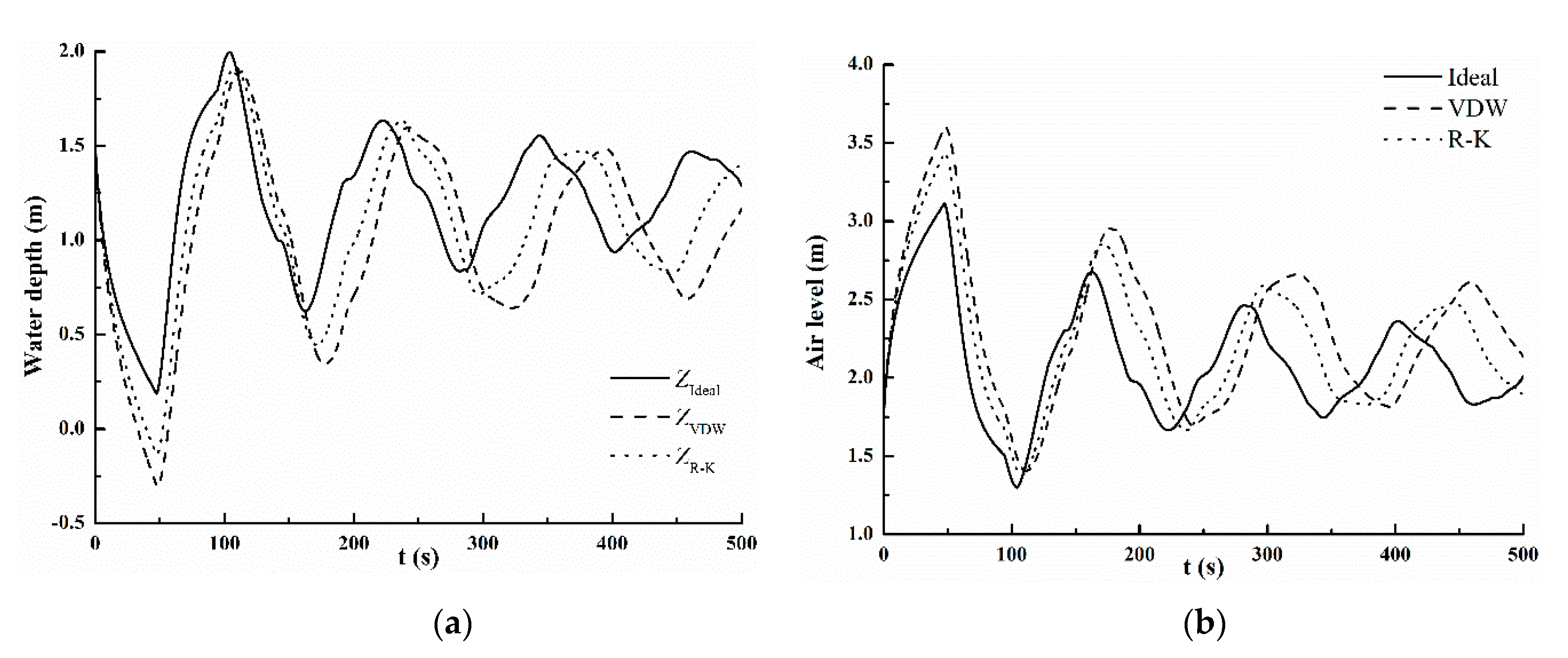
As shown in Figure 3a–c, the pressure adjacent to the pump decreases rapidly as soon as there is pump failure (t = 0), the upstream fluid continually moves downstream together with negative pressure wave until the positive pressure wave reflects back to the source. The water in the air vessel (D_vessel = 2 m) quickly enters the pipe to relieve the pressure reduction, which will result in the water depth dropping, air level rises and air pressure drops in the vessel during the first phase (0~t = 2 L/a = 47.41 s, L is the total length of the pipeline).

The comparison of the fluctuation calculated by three models is discussed. According to Equations (4) and (10), the air pressure in the vessel calculated by the real gas models is always smaller compared to the ideal gas model on the account of non-zero intermolecular attractions i.e., the positive cohesion pressure. Likewise, the corresponding water levels are lower than those of the ideal gas. In addition, since the cohesion pressure of VDW is larger than that of the R–K equation under the same volume, the air pressure calculated by the VDW model is lower than that calculated by the R–K model. Figure 3c shows that the numerical results of air level and pressure oscillations for each gas model are consistent with the above theoretical analysis.

Lower pressure means longer oscillation period. Thus, compared with the pressure fluctuations of the three models, the lag as shown in Figure 3c seems to be compatible with the lower pressure. Figure 3d shows the air pressure ratio during the first phase (0~t = 2 L/a = 47.41 s, L is the total length of the pipeline) in order to avoid the influence of lag. The air pressure ratios ($P_{\mathrm{VDW}}/P_{\mathrm{Ideal}}$ and $P_{\mathrm{RK}}/P_{\mathrm{Ideal}}$) remain nearly stable in first (0–2 s) and drop at last during the first phase. At t = 47.41 s, the air pressure ratio values of $P_{\mathrm{VDW}}/P_{\mathrm{Ideal}}$ and $P_{\mathrm{RK}}/P_{\mathrm{Ideal}}$ are 0.89 and 0.92, respectively.

Table 2 shows that the minimum water depths calculated by the ideal gas model, the VDW model and the R–K model are 0.19 m, −0.3 m and −0.13 m, respectively, the maximum air levels for the three models are 3.11 m, 3.60 m and 3.43 m, respectively, and the minimum air pressures for the three models are 1.46 MPa, 1.30 MPa and 1.35 MPa, respectively. The results in Table 2 show that the real gas models predict the water depth to be critically low, reducing the safe margin required in the air vessel ($Z_{\mathrm{VDW}}-Z_{\mathrm{Ideal}}=0.49\mathrm{m}$, $Z_{\mathrm{RK}}-Z_{\mathrm{Ideal}}=0.32\mathrm{m}$). Hence the necessity for the inclusion of real gas approximations.

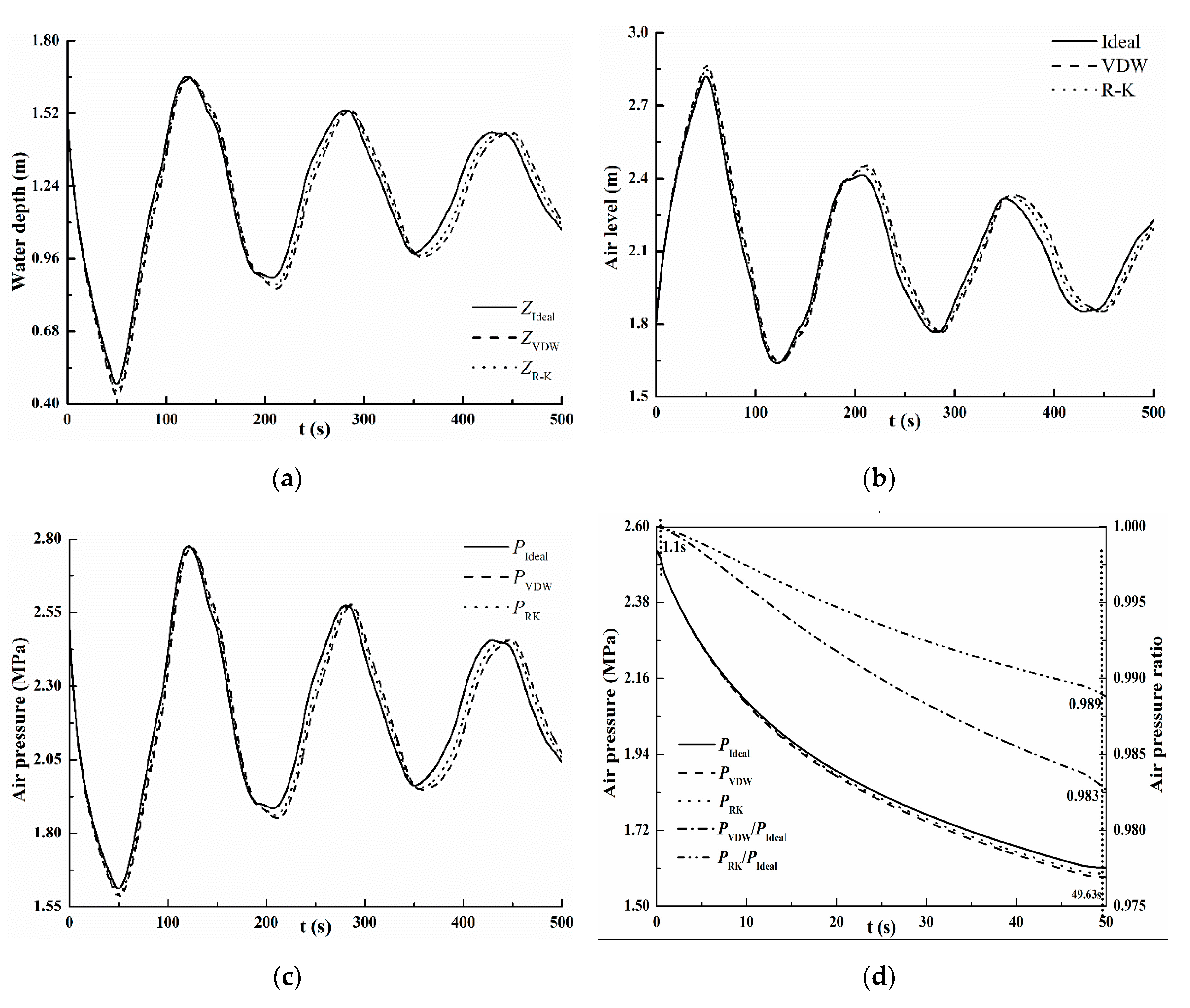
As shown in Figure 4a‒c, the water depth, air level and air pressure curves of the VDW gas model and the R–K gas model are almost coincided with that of the ideal gas model for D_vessel = 3 m. The positive wave reaches the upstream end of the pipe at t = 49.63 s, and the water depths, air levels and air pressures calculated by the ideal air, VDW and R–K models reach the maximum value at 121.11 s, 123.99 s and 122.97 s, respectively, which are almost the same. Figure 4d shows that the air pressure ratios remain almost stable first and drop last along with the air expansion during 0–49.63 s. The cohesion pressure has no significant effect due to the small variation of air volume at the beginning of the transient. Therefore, the pressure ratios is changed but not much during 0–1.1 s. Then, the influence of cohesion pressure is becoming increasingly obvious. At t = 49.63 s, the minimum values of $P_{\mathrm{VDW}}/P_{\mathrm{Ideal}}$ and $P_{\mathrm{RK}}/P_{\mathrm{Ideal}}$ are 0.983 and 0.989. As seen from Table 2, the pressure and level differences are now much smaller compared to the ideal gas (≈1%), as a consequence of the negligible influence of the interatomic attractions in the high-pressure regime (cohesion pressure in Equations (4) and (8) tend to zero).

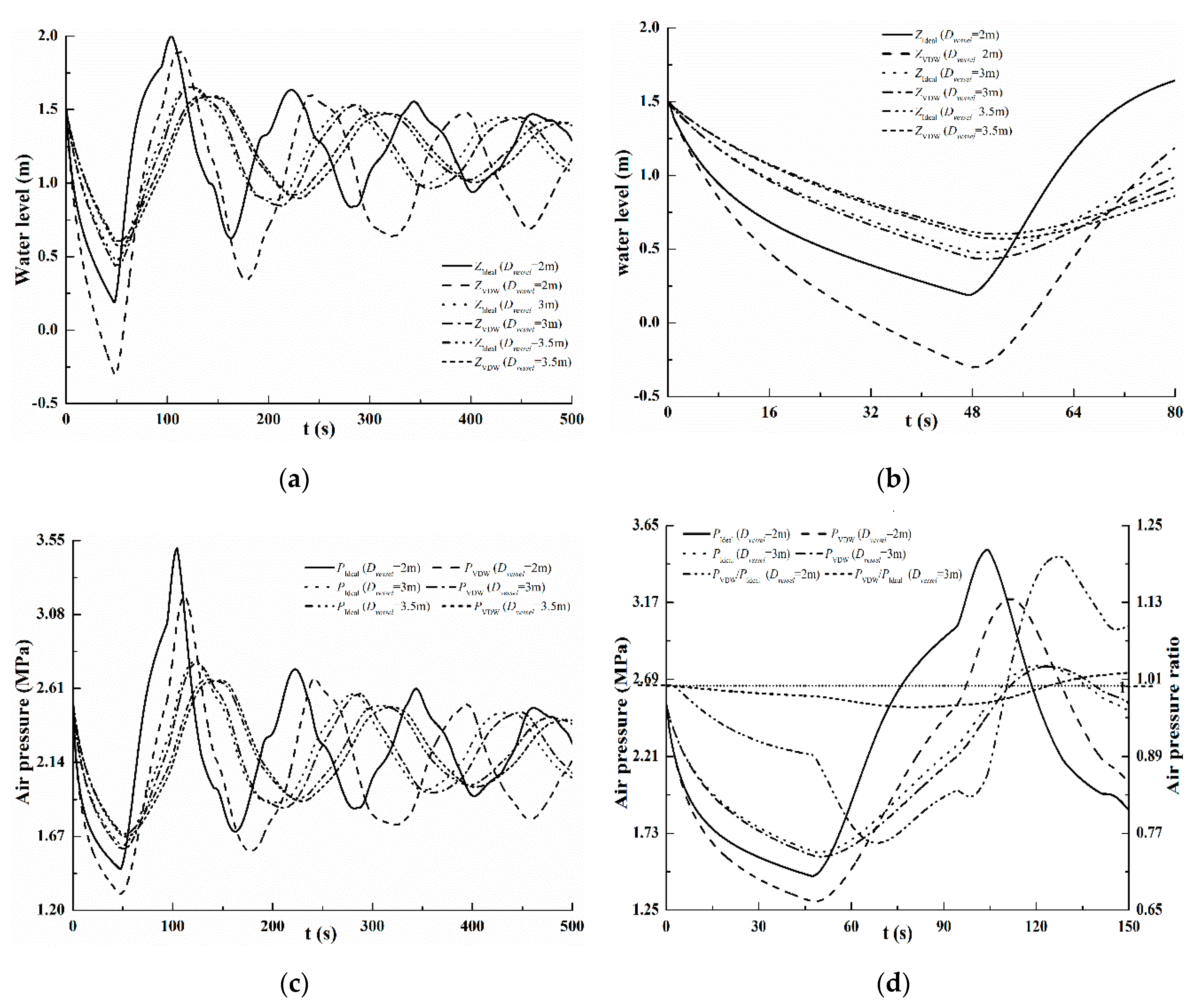
Comparison between the VDW gas model and the ideal gas model for varying diameters are conducted, which are presented in Figure 5a–d. The results show that fluctuations of water depth, air pressure and air pressure ratio are more violent with the smaller vessel diameter. The differences of the water depths, air pressures, air levels and air pressure ratio between the ideal model and the VDW model are larger when the vessel diameter is smaller. Note the asymmetry in the upward and downward oscillations (including the sudden changes in the water depth and air pressure, Figure 5a,c), akin to hysteresis. The smaller the diameters, the shorter are the periods of the fluctuations of water depth and air pressure. For the initial air-vessel diameter ranging from 2 m to 3 m, Figure 5d shows that the values of air-pressure ratios are almost lower than 1 during the first period. After the first phase, the trends of air-pressure ratios changes due to the lag. The ratios exceed 1 after the crossover of the curves (around 116 s, Figure 5d). However, the corresponding points of the pressure curves corrected for the lag are always lower for the real gases, Figure 5c.

6. Conclusions

In this study, a simplified R–K gas polytropic equation is proposed and derived under the assumption of the total volume occupied by air molecules themselves could be negligible.

The effect of cohesion pressure is verified by theoretically and numerically studying the comparison between ideal, VDW and R–K gas equations for the cases of different vessel diameters. The results show that cohesion pressure of real air in the small-volume air vessel is more significant with respect to that in the large volume air vessel. For the small volume vessel, the real gas models predict critically low water levels (≈0.5 m), so that an adequate safety margin can be provided in the operation of pump-air vessel downstream systems.

This study provides theoretical and numerical support for the influence of cohesion pressure in small-volume vessel. However, it must be noted that the practical project introduced in this paper is still under construction, so no measured data are available to make a comparison with the results. Therefore, future research will be carried out to further verify the impact of cohesion pressure in the air vessel after the measured data are obtained in the future.

References

- Sun, Q.; Wu, Y.B.; Xu, Y.; Jang, T.U. Optimal Sizing of an Air Vessel in a Long-Distance Water-Supply Pumping System Using the SQP Method. J. Pipeline Syst. Eng. Pract. 2016, 7. [Google Scholar] [CrossRef]
- Clarke, D.S. Surge suppression—A warning. In Proceedings of the International Conference on the Hydraulics of Pumping Stations, Manchester, UK, 17–19 September 1985; pp. 39–54. [Google Scholar]
- Liang, X.; Liu, M.Q.; Zhang, J.G. Protection study on water hammer of pipelines by air vessel. Drain. Irrig. Mach. 2005, 23, 16–18. [Google Scholar]
- Wan, W.Y.; Huang, W.R. Investigation of fluid transients in centrifugal pump integrated system with multi-channel pressure vessel. J. Press. Vessel Technol. 2013, 135, 061301. [Google Scholar] [CrossRef]
- Lee, T.S. A numerical method for the computation of the effects of an air vessel on the pressure surges in pumping systems with air entrainment. Int. J. Numer. Methods Fluids 1998, 28, 703–718. [Google Scholar] [CrossRef]
- Lee, T.S. Effects of air entrainment on the ability of air vessels in the pressure surge suppressions. J. Fluids Eng. 2000, 122, 499–504. [Google Scholar] [CrossRef]
- Lee, T.S.; Low, H.T.; Weidong, H. The Influence of Air Entrainment on the Fluid Pressure Transients in a Pumping Installation. Int. J. Comput. Fluid Dyn. 2003, 17, 387–403. [Google Scholar] [CrossRef]
- Wang, L.; Wang, F.J.; Zou, Z.C.; Li, X.N.; Zhang, J.C. Effects of air vessel on water hammer in high-head pumping station. In Proceedings of the 6th International Conference on Pumps and Fans with Compressors and Wind Turbines IOP, Beijing, China, 19–22 September 2013; Volume 52, pp. 7–13. [Google Scholar] [CrossRef] [Green Version]
- Wood, D.J. Pressure surge attenuation utilizing an air vessel. J. Hydr. Div. 1970, 96, 1143–1156. [Google Scholar]
- Sun, Q.; Wu, Y.B.; Xu, Y.; Jang, T.U. Flux Vector Splitting Schemes for Water Hammer Flows in Pumping Supply Systems with Air Vessels. J. Harbin Inst. Technol. 2015, 22. [Google Scholar] [CrossRef]
- Yang, K.L. Hydraulic Transients and Regulate in Power and Pumping Station; Water Conservancy and Hydropower Press: Beijing, China, 2000. (In Chinese) [Google Scholar]
- Gjetvaj, G.; Tadić, M. The Effect of Water Hammer on Pressure Increases in Pipelines Protected by an Air Vessel. J. Tech. Gaz. 2014, 21, 479–484. [Google Scholar]
- Kim, S.G.; Lee, K.B.; Kim, K.Y. Water hammer in the pump-rising pipeline system with an air vessel. J. Hydrodyn. 2014, 26, 960–964. [Google Scholar] [CrossRef]
- Jones, J.B.; Dugan, R.E. Engineering Thermodynamics; Prentice Hall Inc.: New Jersey, NJ, USA, 1996. [Google Scholar]
- Moran, M.J.; Shapiro, H.N. Fundamentals of Engineering Thermodynamics, 3rd ed.; John Wiley & Sons Inc.: New York, NY, USA, 1995. [Google Scholar]
- Zhong, W.; Xiao, C.M.; Zhu, Y.K. Modified Van der Waals equation and law of corresponding states. Phys. A 2016, 471, 295–300. [Google Scholar] [CrossRef] [Green Version]
- Cowan, B. Topics in Statistical Mechanics; Imperial College Press: London, UK, 2005. [Google Scholar]
- Van der Waals, J.D. On the Continuity of the Gaseous and Liquid States. Ph.D. Thesis, Universiteit Leiden, Leiden, The Netherlands, 1873. [Google Scholar]
- Plischke, M.; Bergersen, B. Equilibrium Statistical Physics; World Scientific Publishing Co. Pvt. Ltd.: Singapore, 2005. [Google Scholar]
- Redlich, O.; Kwong, J.N.S. On the thermodynamics of solutions, V. An equation of state, Fugacities of gaseous solutions. Chem. Rev. 1949, 44, 233–244. [Google Scholar] [CrossRef] [PubMed]
- Gray, R.D.; Rent, N.H.; Zudkevitch, D. A modified Redlich-Kwong equation of state. Am. Inst. Chem. Eng. 1970, 16, 991–998. [Google Scholar] [CrossRef]
- Shin, Y.G. Estimation of instantaneous exhaust gas flow rate based on the assumption of a polytropic process. J. Automob. Eng. 2001, 25, 637–643. [Google Scholar] [CrossRef]
- Najm, H.; Azoury, P.H.; Piasecki, M. Hydraulic ram analysis: A new look at an old problem. J. Power Energy 1999, 213, 127–141. [Google Scholar] [CrossRef]
- Filipan, V.; Virag, Z.; Bergant, A. Mathematical modelling of a hydraulic ram pump system. J. Mech. Eng. 2003, 49, 137–149. [Google Scholar]
- Chaudhry, M.H. Applied Hydraulic Transients, 3rd ed.; Van Nostrand Reinhold: New York, NY, USA, 2014. [Google Scholar]
- Svee, R.; Techn, D. Surge vessel with enclosed compressed air cushion. In Proceedings of the 1st International Conference on Pressure Surges, BHRA Fluid Engineering, Cranfield, UK, 6–8 September 1972; pp. 15–24. [Google Scholar]
- Goodall, D.C.; Kjørholt, H.; Tekle, T.; Broch, E. Air cushion surge vessels for underground power plants. Water Power Dam. Constr. 1989, 40, 29–34. [Google Scholar] [CrossRef]
- Borg, J.E.; Steward, E.H. Moose river air vessel design and performance. In Proceedings of the Conference Proceeding, Waterpower’89, U.S. Army Corps of Engineers, Buffalo District, New York, NY, USA, 23–25 August 1989; pp. 567–576. [Google Scholar]
- Zhou, L.; Liu, D.; Karney, B. Investigation of hydraulic transients of two entrapped air pockets in a water pipeline. J. Hydraul. Eng. 2013, 139, 949–959. [Google Scholar] [CrossRef]
- Zhou, L.; Liu, D.; Karney, B.; Wang, P. Phenomenon of white mist in water rapidly filling pipeline with entrapped air pocket. J. Hydraul. Eng. 2013, 139, 1041–1051. [Google Scholar] [CrossRef]
- Vereide, K.; Tekle, T.; Nielsen, T.K. Thermodynamic Behavior and Heat Transfer in Closed Surge Tanks for Hydropower Plants. J. Hydraul. Eng. 2015, 141. [Google Scholar] [CrossRef] [Green Version]
- Fan, B.Q.; Zhang, J.; Suo, L.S.; Liu, D.Y. Stability analysis on small fluctuation of the system with air-cushion surge vessel for hydropower station. Water Resour. Hydropower Eng. 2005, 36, 114–115. [Google Scholar]
- Jin, H. Further discussion of Van der Waals gas. J. Gansu Educ. Coll. 2003, 17, 59–62. [Google Scholar]
- Borgnakke, C.; Sonntag, R.E. Thermodynamic and Transport Properties; John Wiley & Sons Inc.: New York, NY, USA, 1997. [Google Scholar]
- Yunus, A.C.; Michael, A.B. Thermodynamic: An Engineering Approach, 3rd ed.; McGraw-Hill, Inc.: London, UK, 1995. [Google Scholar]