Streamflow Variability in Colombian Pacific Basins and Their Teleconnections with Climate Indices

Abstract

Oceanic-atmospheric phenomena of different time scales concurrently might affect the streamflow in several basins around the world. The Atrato River Basin (ARB) and Patía River Basin (PRB) of the Colombian Pacific region are examples of such basins. Nevertheless, the relations between the streamflows in the ARB and PRB and the oceanic-atmospheric factors have not been examined considering different temporal scales. Hence, this article studies the relations of the climate indices and the variability of the streamflows in the ARB and PRB at interannual and decadal timescales. To this, the streamflow variability modes were obtained from the principal component analysis (PCA); furthermore, their linear dependence with indices of the El Niño/Southern Oscillation (ENSO), precipitation (PRP), the Choco low-level jet (CJ), and other indices were quantified through (a) Pearson and Kendall’s tau correlations, and (b) wavelet transform. The PCA presented a single significant mode for each basin, with an explained variance of around 80%. The correlation analyses between the PC1s of the ARB and PRB, and the climate indices showed significant positive (negative) high correlations with PRP, CJ, and Southern Oscillation Index (SOI) (ENSO indices). The wavelet coherence analysis showed significant coherencies between ENSO and ARB: at interannual (2–7 years) and decadal scale (8–14), preferably with the sea surface temperature (SST) in the east and west Tropical Pacific Ocean (TPO). For PRB with the SST in the central and western regions of the TPO in the interannual (4–8 years) and decadal (8–14 years) scales, the decreases (increases) in streamflow precede the El Niño (La Niña) events. These results indicate multiscale relations between the basins’ streamflow and climate phenomena not documented in previous works, relevant to forecast the extreme flow events in the Colombian Pacific rivers and for planning and implementing strategies for the sustainable use of water resources in the basins studied.

1. Introduction

Knowing the variability of hydroclimatological variables like rainfall and streamflow is fundamental for understanding water cycle dynamics [1]. According to Jiang et al. [2], this variability is associated with climate change effects and large-scale climate anomalies. Thus, by getting a better understanding of the teleconnection between different climate indices and hydroclimatological variables may improve the modeling of water systems and can, in turn, optimize water resource management in a given region [3].

Of the variables associated with the water cycle, streamflow acts as a relevant index for a region’s hydroclimatological variability [4] and is related to the interaction between climate conditions and the basin’s hydrogeological and morphometrical features [5], acting as a variable that spatiotemporarily integrates precipitation, evapotranspiration, and other water balance variables. Moreover, the variability of streamflow is related to large-scale teleconnection patterns and has been studied in different regions worldwide as Africa [6,7], North America [4,8,9,10,11], Europe [12,13,14], Asia [15,16], and South America [5,17,18,19,20,21,22,23,24,25].

Colombia presents some orographic characteristics and hydroclimate conditions that need to be carefully analyzed because they influence the genesis and dynamics of regional climate variability. One of the most interesting regions is the Colombian Pacific, also known as the Colombian Biogeographic Chocó (henceforth CBC), which is modulated by the ocean-atmospheric processes between the Colombian Andes and the eastern Pacific Ocean [26]. This region is considered one of the rainiest on our planet because its mean annual rainfall exceeds 12,500 mm [27,28], and it is one of the hotspots of the world’s biodiversity [29,30]. Therefore, gaining a better understanding on the influence of the large-scale phenomena on the temporal variability of streamflows in the basins of the CBC is especially relevant for hydrological modeling, the all-round management of climate-related risks, and for dealing with water resources in regions of particular environmental interest [4,25,31].

Given the geographic location of Colombia, its hydroclimatology is directly influenced by the regional moisture transport processes driven by the confluence of global and local factors. Due to its proximity to the Equator the seasonality of rainfall and streamflows is mainly defined by the migration of the Inter Tropical Convergence Zone (ITCZ). Additionally, the proximity of this country to the Pacific Ocean makes it sensitive to climatic phenomena such as El Niño/Southern Oscillation (ENSO) [32,33,34] and the Choco low-level jet (CJ) [28] with serious consequences for the population and water/energy resources. Several studies have established that the warm phase of ENSO (EN) generally brings lower than average rainfall and increase in the air temperature and therefore negative anomalies of flow in Colombia, and the cold phase of ENSO (LN) above average rainfall and increased river discharges and landslide [20,35,36]. In addition, the CJ brings much moisture to the Pacific coast of Colombia and explains the world-record breaking precipitation area over this region. Upon entering the continent, the CJ is lifted by the orography of the Western Cordillera of the Colombian Andes, interacts with the easterly trade winds, and contributes to enhance deep convection [37,38].

According to several authors the main teleconnections between large-scale phenomena and the hydroclimatological variables in Colombia have been identified through indices linked to the ENSO: Southern Oscillation Index (SOI), multivariate ENSO index (MEI), and Niño sea surface temperature (SST) in regions Niño1+2 (SST1+2), Niño3 (SST3), Niño3.4 (SST3.4), and Niño 4 (SST4) [20,34,39,40,41,42,43,44,45]. In addition, other phenomena such as the Pacific decadal oscillation (PDO), North Atlantic oscillation (NAO), and Tropical North Atlantic (TNA) variability might also affect the Colombian climate [39,46]. In this way, studies in the Colombian territory have made significant advances in the influence of large-scale phenomena with hydroclimatological variability in different regions; however, the temporal persistence of these relations is not yet wholly understood.

The main objective of this research is to study the influence of large-scale climate phenomena on the variability of the streamflows of the Atrato River Basin (ARB) and Patía River Basin (PRB) in the Colombian Pacific region, through the quantification of the linear correlations and the Wavelet coherence analysis. Hence, this article is arranged as follows: Section 2 describes the study area and presents the data. Section 3 describes the methodology, which includes filling missing data. Section 3 offers the results and discussion. Finally, Section 4 sets out the conclusions.

2. Materials and Methods

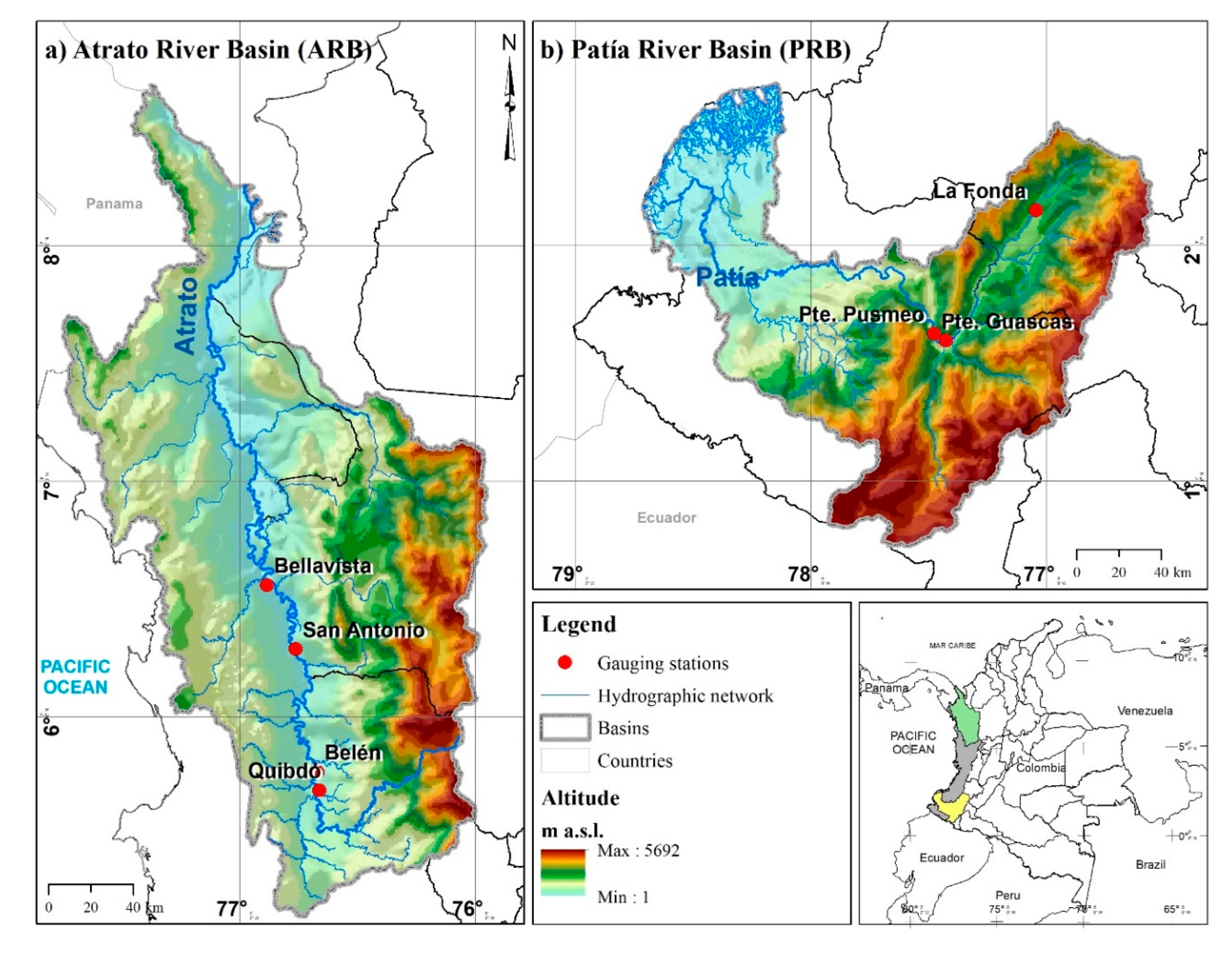
2.1. Study Area

The study area comprises the ARB and PRB, which lie in the far north and far south of the CBC, respectively (Figure 1). The ARB is characterized by a drainage of 37,731.8 km² with a mean discharge of 4137 m³·s⁻¹ and is the fastest flowing river in the world [47]. It rises in the Western mountain range of the Colombian Andes at 3800 m.a.s.l., and it flows into the Caribbean Sea after a stretch of more than 600 km [30]. The Patía River rises in the Colombian massif on the western slopes of the Central mountain range of the Colombian Andes. Its basin covers an approximate surface area of 23,909 km². It lies in southeast of Colombia, is 360 km long, and its mean discharge is 383 m³·s⁻¹ [30].

2.2. Streamflow Data

Monthly streamflow time series for the 1981–2016 period corresponding to four flow-gauge stations of the ARB and three of the PRB provided by Instituto de Hidrología, Meteorología y Estudios Ambientales (IDEAM) of Colombia were used. The hydrometric characteristics and statistical details of streamflows are presented in

Table 1. Description of the flow gauge stations and discharges used in the study.

Station	ID	Mean (m3·s−1)	Std. Dev. (m3·s−1)	Coef. of Var.	Missing Data %	River Basin	Drainage Area (km2)
Belén	BEL	1062.5	257.9	0.25	5.3	Atrato (37,731.8 km2)	617.3
Quibdó	QUI	1023.1	229.0	0.22	14.8		4845.5
San Antonio	SAN	1937.0	431.2	0.22	4.4		560.8
Bellavista	BELL	2524.0	626.3	0.25	2.8		6207.3
Guascas	GUA	203.2	130.4	0.64	30.6	Patía (23,909.5 km2)	15,177.4
La Fonda	FON	62.4	47.8	0.77	17.6		1444.1
Pusmeo	PUS	299.5	165.3	0.55	31.5		4112.6

. These flow-gauge stations were selected for their relatively large drainage areas and long-term records.

2.3. Climate Indices

Eleven climate indices were selected (

Table 2. Climate indices used in the Colombian Biogeographic Chocó (CBC) region and publications.

Climate Indices	References
SOI	Carvajal et al. [56], Poveda et al. [39], Rojo and Carvajal, [42], Ávila et al. [57]
MEI	Poveda et al. [39], Poveda, [26], Puertas and Carvajal, [58], Ávila et al. [57], Loaiza et al. [34]
ONI	Ávila et al. [57], Enciso et al. [21], Loaiza et al. [34]
SST1+2	Puertas and Carvajal, [58], Rodríguez-Rubio, [43]
SST3	Carvajal et al. [56], Poveda et al. [20], Rodríguez-Rubio, [43]
SST3.4	Carvajal et al. [56], Tootle et al. [59], Puertas and Carvajal, [58], Ávila et al. [57], Loaiza et al. [34]
SST4	Carvajal et al. [56], Puertas and Carvajal, [58], Poveda et al. [20]
PDO	Poveda and Mesa, [60], Poveda et al. [19], Poveda et al. [39], Tootle et al. [59], Loaiza et al. [34]
NAO	Poveda et al. [39], Hurtado, [61], Hoyos et al. [62]
TNA	Carvajal et al. [56]
CJ	Poveda and Mesa, [63], Poveda, [26], Sierra et al. [64], Durán-Quesada et al. [65]

) considering previous results that identified the physical relations among large-scale climate phenomena and Colombian hydroclimatology. To analyze the interannual scale associated mainly with ENSO there were used climate indices such as the SOI, calculated as the difference in the sea level pressure (SLP) anomalies between Tahiti and Darwin. MEI is another index defined as the linear combination of six variables from the tropical Pacific: SLP, zonal, and meridional components of the surface wind, SST, and total cloud cover [48]. Oceanic Niño Index (ONI) is calculated as the 3-month moving average of SST anomalies in the Niño3.4 region [49]. The SST indices are the average of SST in Tropical Pacific Ocean (TPO) regions: Niño1+2 (0–10° S, 90°–80° W), Niño3 (5° S–5° N, 90°–150° W), Niño3.4 (5° N–5° S, 170°–120° W), and Niño4 (5° N–5° S, 160° E–150° W). The climate indices used in this study were provided by National Oceanic and Atmospheric Administration (NOAA) website (https://www.esrl.noaa.gov/psd/data/climateindices/list/).

For the decadal scale, the PDO index was used. This index is defined as the principal component time series of the leading empirical orthogonal function (EOF) mode of the SST anomalies in the North Pacific Ocean, poleward of 20° N [50] and was taken from the Joint Institute for the Study of the Atmosphere and Ocean (JISAO) website (http://research.jisao.washington.edu/pdo/). The NAO was also used and represents the differences in normalized atmospheric pressures between the Azores islands and Iceland [51], and the TNA index is the average of the monthly SST anomalies in the eastern TNA Ocean limited from 5.5° N to 23.5° N and from 15° W to 57.5° W, obtained from the NOAA website.

The CJ index, estimated as the average zonal wind at 925 hPa for the region between 2° N–7° N and 80° W [28,35,52,53] was also used. Zonal wind data were obtained from the European Centre for Medium-Range Weather Forecasts Interim Reanalysis (ECMWF/ERA-I, 2018) [54].

The areal precipitation data of the basins under study correspond to monthly precipitation data extracted from the Climate Hazards Group InfraRed Precipitation with Station Data (CHIRPS, 2018), version v2.0, created and managed by the U.S. Geological Survey and University of California, Santa Barbara. For this data, the horizontal resolution of 0.25° was used [55]. All indices were obtained for the period 1981–2016.

2.4. Filling Missing Data

The monthly streamflow series employed for the analysis presented the missing data in the proportions indicated in Table 1. These missing data were estimated by the nonlinear principal component analysis (NLPCA) method proposed by Scholz et al. [66]. This method was applied to estimate rainfall missing data by Miró et al. [67], who evaluated 10 methodologies to estimate missing data in daily and monthly rainfall data, and reported NLPCA as the best-performing method. Furthermore, this methodology was used by Canchala et al. [68], who estimated missing data of monthly rainfall in southwestern Colombia using artificial neural networks (ANN). NLPCA is the nonlinear generalization of a principal component analysis (PCA) employing ANN. The NLPCA algorithm used here is found in the nonlinear PCA toolbox (http://www.nlpca.org/matlab.html). Details about this process are found in Scholz et al. [66,69]. In order to evaluate the performance of this method, the estimated and the original observed data series were statistically compared using the relative root mean square error (RRMSE), given as:

$$RRMSE=\frac{\sqrt{\frac{1}{n}{{\displaystyle \sum }}_{i=1}^n{\left(s_i-m_i\right)}^2}}{\overline{M}}$$

(1)

where $s$ refers to the estimated values, $m$ denotes the observed values, $\overline{M}$ is their sample mean, and n corresponds to sample size.

2.5. Principal Component Analysis

The PCA is a well-established linear statistical method frequently employed to analyze hydroclimatological data, such as streamflows and rainfall [5,67,70,71]. Its objective is to reduce the size of the time series to some main orthogonal principal components (PCs) that explain most of the variability of the original variables [72] with minimum loss of information [73]. In the present research work, the PCA method was used to represent and characterize the dominant patterns of variability of streamflows of the ARB and PRB. The PCs with eigenvalues above 1 were selected, as suggested by Jolliffe [74] and Preisendorfer [75].

Before performing the monthly PCA, the streamflow values were converted into anomalies by deducting the mean monthly climatological value for each month from the monthly values to, thus, eliminate the annual cycle. Then the determining correlation factor was estimated, followed by the Kaiser–Meyer–Olkin (KMO) index to evaluate multicollinearity among stations [76]. Subsequently, a PCA of the annual, maximum, and minimum streamflow data series was performed to analyze the correlations with climate indices.

2.6. Kendall’s Tau and Pearson Correlation Coefficient

The correlation between streamflows and climate indices were estimated by Kendall’s Tau correlation using monthly, annual, maximum, and minimum values for the 1981–2016 period. The Kendall’s tau $\left(\tau \right)$a nonparametric correlation coefficient is a useful estimator of the degree of dependence between two variables, which can be used to evaluate the number of accordance and discordance in paired variables that is done within a range of data [77,78]:

$${\tau }_b=\frac{n_c-n_d}{\sqrt{\left(T_0-T_1\right)\left(T_0-T_2\right)}}$$

(2)

where ${\tau }_b$ is the Kendall tau-b coefficient, $T_0=n\left(n-1\right)/2,T_1={\displaystyle \sum }_k{t}_k\left(t_k-1\right)/2$ and $T_2={\displaystyle \sum }_l{u}_l\left(u_l-1\right)/2,t_k$ is the number of $x$ values in the kth group of linked $x$ values, $u_l$ is the number of $y$ values in the lth group of linked $y$ values, $n$ is the number of observations, $n_c$ is the number of accordant pairs, and $n_d$ is the number of disaccordant pairs.

The sensitivity of the streamflows response was evaluated on a monthly scale through cross-correlations with the climate indices estimated for each month by considering time lags of up to 12 months based on the premise that lags can occur between precipitation and run-off. The cross-correlations were estimated by Pearson correlation, considering that macroclimate variables precede the hydrological variable. For the present research work, the significance of the correlations was identified by the Student’s t-test for a 95% confidence level ($\alpha =0.05)$.

2.7. Wavelet Transform

Wavelet transform has been widely used in different research works worldwide to analyze time series of ENSO [79], to identify and describe the variability in annual streamflows [4], and interannual, decadal, and multidecadal climate oscillations of annual discharge [80]. This method was also used to understand mechanisms driving streamflow variability at all timescales [81], and to analyze precipitation extremes and their teleconnections with large-scale climate anomalies [82], among others.

After obtaining the streamflow PC1s, they were decomposed over a space of time and frequency by the Morlet Wavelet analysis [79,83]. Morlet Wavelet is a complex exponential that is modulated by a Gaussian window:

$$\psi \left(t\right)=e^{i{\omega }_0\eta }{e}^{-\frac{{\eta }^2}{2}}$$

(3)

where $\eta =t/s$, t is time, $s$ is the wavelet scale according to time ($s=2/\partial t$) and ${\omega }_0$ is nondimensional frequency [79,83]. The analysis was carried out by the computational procedure of wavelet analyses described by Torrence and Compo [79]. To avoid edge effects and by employing fast Fourier transform, the series were completed with zeros, and their total increased length was obtained up to the next power of 2. The wavelet function in each scale was normalized to get the unit energy, which guarantees that the Wavelet Transform is comparable on many scales. The global wavelet power (GWP) spectrum for a given $s$ scale is the mean time of all local wavelet power spectra (WPS) and is quantified such as [79]:

$${\overline{W}}^2\left(s\right)=\frac{1}{N}{\displaystyle \sum }_{n=0}^{N-1}{\left|W_n\left(s\right)\right|}^2$$

(4)

The wavelet coherence and phase difference analysis was also performed to compare the PC1s and climate indices by following the methodology proposed by Grinsted et al. [84] and Torrence and Webster [85]. Given two time series, X(t) and Y(t), with their respective wavelet transforms, $W^X\left(t,s\right)$ and $W^Y\left(t,s\right)$, the cross-wavelet spectrum is defined as $W^{XY}\left(t,s\right)=W^X\left(t,s\right)W^{Y*}\left(t,s\right)$, where (*) indicates the conjugated complex. Squared wavelet coherence is defined as the square of the smoothed cross-wavelet spectrum module normalized by the smoothed wavelet spectrum:

$$R_n^2\left(s\right)=\frac{{|\langle s^{-1}{W}^{XY}\left(t,s\right)\rangle |}^2}{\langle s^{-1}{\left|W^X\left(t,s\right)\right|}^2\rangle \langle s^{-1}{\left|W^Y\left(t,s\right)\right|}^2\rangle }$$

(5)

where 〈〉 is a smoothing in time and the scale. Factor s⁻¹ is used to convert the square of the wavelet coherence into energy density. Wavelet coherence accurately represents the (normalized) covariance between both time series because the wavelet transform maintains the variance [79]. The phase difference in the wavelet coherence is indicated as follows:

$${\mathsf{\Phi }}_n\left(s\right)=ta{n}^{-1}\left(\frac{\Im m\{\langle s^{-1}{W}^{XY}\left(t,s\right)\rangle \}}{\Re e\{\langle s^{-1}{W}^{XY}\left(t,s\right)\rangle \}}\right)$$

(6)

where $\left(\Im m\right)$ and $\left(\Re e\right)$ are the imaginary and real parts of $W^{XY}\left(t,s\right)$, respectively. The statistical significance level of the wavelet coherence has to be determined using Monte Carlo methods [84].

3. Results and Discussion

3.1. Completing the Missing Data

Figure 2 provides the results obtained from estimating the missing data from the two flow-gauge stations in the ARB and PRB using NLPCA. The RRMSE in the missing data estimation corresponds to 0.03 (≈[202–4156 m³·s⁻¹] range of streamflows) and 0.39 (≈[4.1–1006 m³·s⁻¹]) for the ARB and the PRB, respectively. In addition, this also provides the estimated streamflows vs. the observed streamflows for flow-gauge stations Quibdó and Pusmeo, which recorded the highest percentage of missing data (14.8% and 31.5%; Table 1) for the ARB and the PRB, respectively. A generally wider variation is observed in the streamflow series for Patía than for Atrato (Figure 2), whose performance is consistent with the estimated variation coefficients found in Table 1.

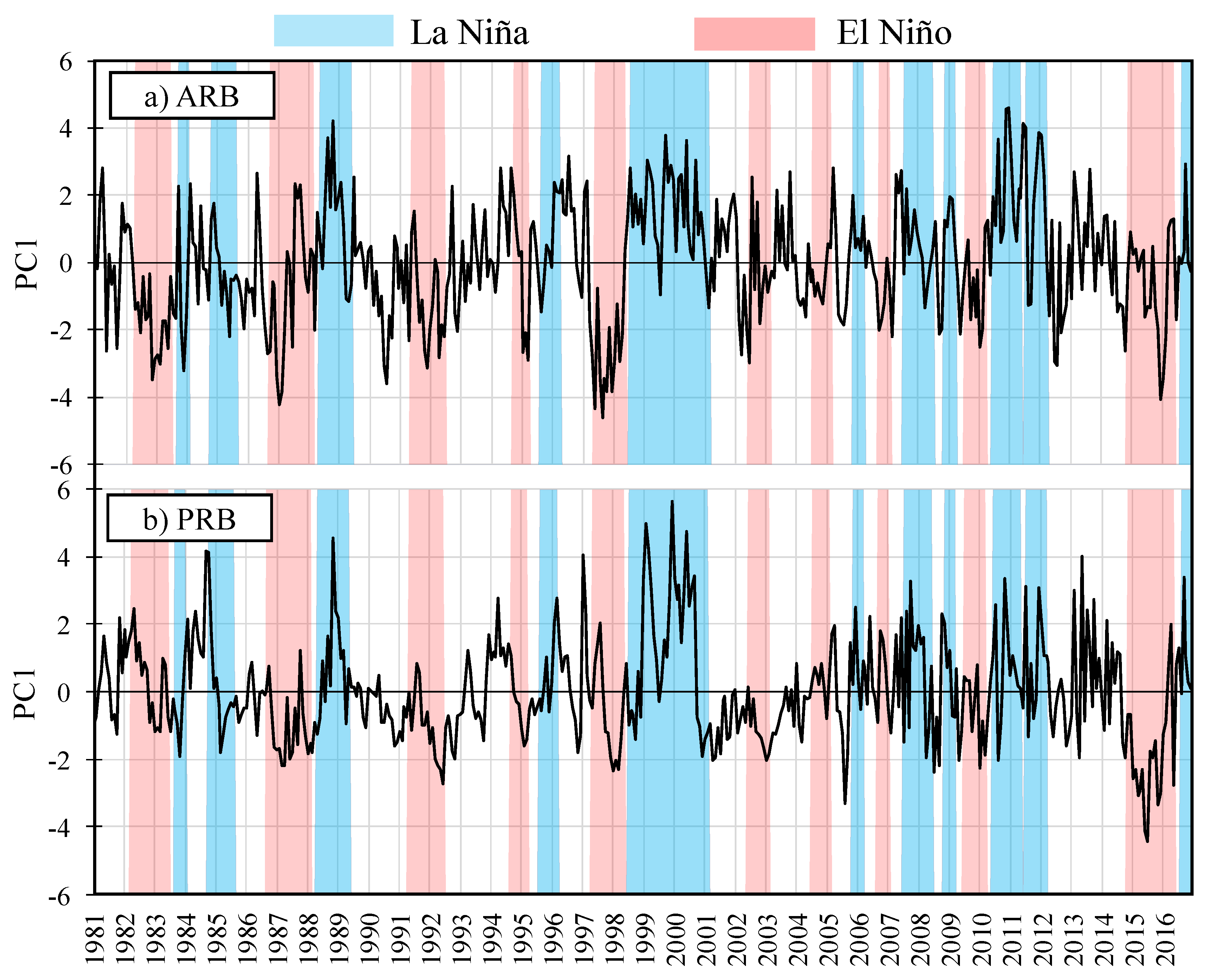
3.2. Principal Component Analysis

The KMO Index estimated for the monthly streamflow series corresponded to 0.78 and 0.61 for the ARB and the PRB, respectively. According to Diaz and Morales [86], a KMO measure above 0.60 is tolerable for factor analysis purposes and, in our case, indicated high multicollinearity among the monthly records of the studied basins flow-gauge stations and the feasibility of performing PCAs.

The PCA results indicate a single significant PC for each basin with eigenvalues above 1 (

Table 3. Explained variance and eigenvalue of the first three principal components at each basin.

PCs	ARB		PRB
	Exp. Var (%)	Eigenvalue	Exp. Var (%)	Eigenvalue
1	75.48	3.02	79.03	2.37
2	15.41	0.61	19.16	0.57
3	6.4	0.25	1.81	0.05

). The selected PCs explained around 80% of the variance of the original data for ARB and PRB. The percentage of explained variance was acceptable given the number of flow-gauge stations in each basin and the complex nature of the studied variable. Likewise, the analysis of the PCs of the annual, maximum, and minimum streamflows indicated a single significant PC with eigenvalues above 1 for each case.

Figure 3 shows the time series of the first principal components (PC1s) for ARB and PRB. Positive (negative) values for the two PC1s, during the 1988–1989, 1998–1999, and 2010–2011 (1997–1998 and 2015–2016) periods coincided with the LN (EN) events recorded by Trenberth [87] and Tedeschi et al. [32]. These events have been related with an increase (reduction) in rainfall, soil moisture, and streamflows in Colombia [20,21,57].

The above-mentioned events strongly impacted the Colombian territory. The 1997–1998 EN had a particularly strong effect on ecosystems, agriculture, energy production, and other sectors of economic development in Colombia (IDEAM, 2002). The 2010–2011 LN caused flooding, storms, and landslides, which mainly affected the Colombian Pacific region [62,88]. During 1997–1998 EN, northern areas of South America suddenly received less rainfall, conversely to the increased rainfall recorded in the south-easterly part of the continent due to the presence of an anomalous Walker cell with its descending branch between 10° N and 10° S in the South American continent and its ascending branch over the eastern Pacific Ocean [33]. The 2010–2011 LN effects were recorded in northern parts of South America and were established by anomalies induced by ENSO in the eastern Pacific, the Caribbean Sea, and the North Atlantic, and by the intrinsic variability of the SST anomalies in the Atlantic Ocean [35].

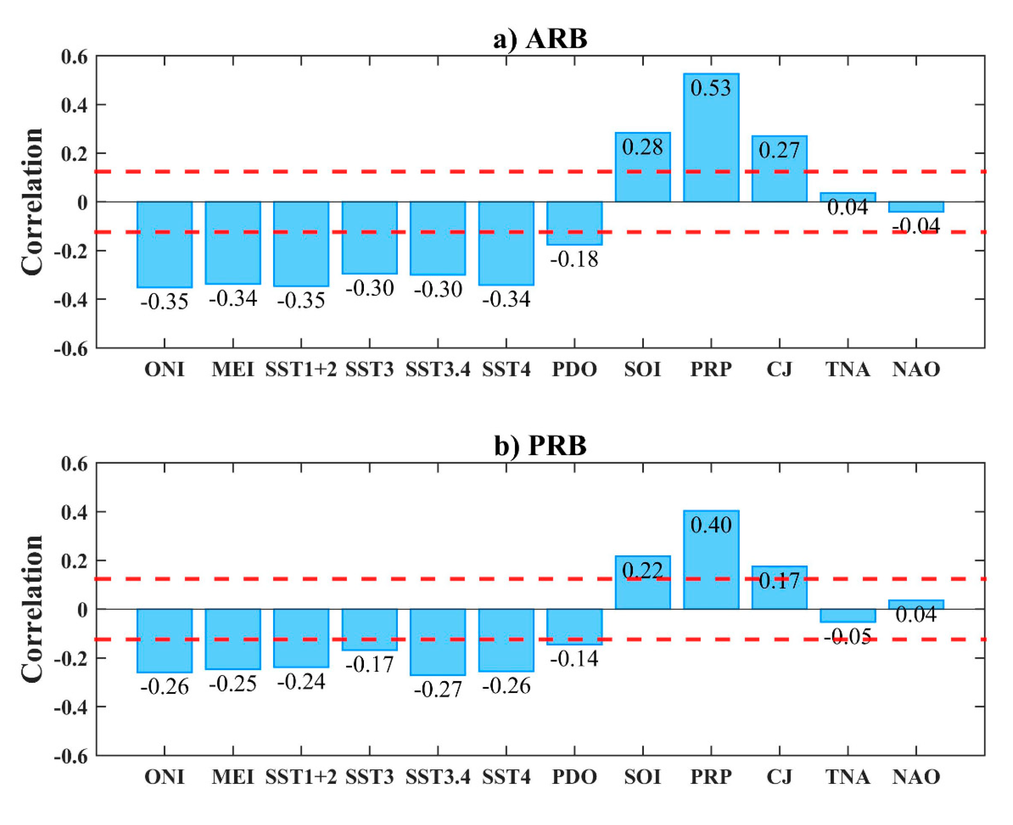
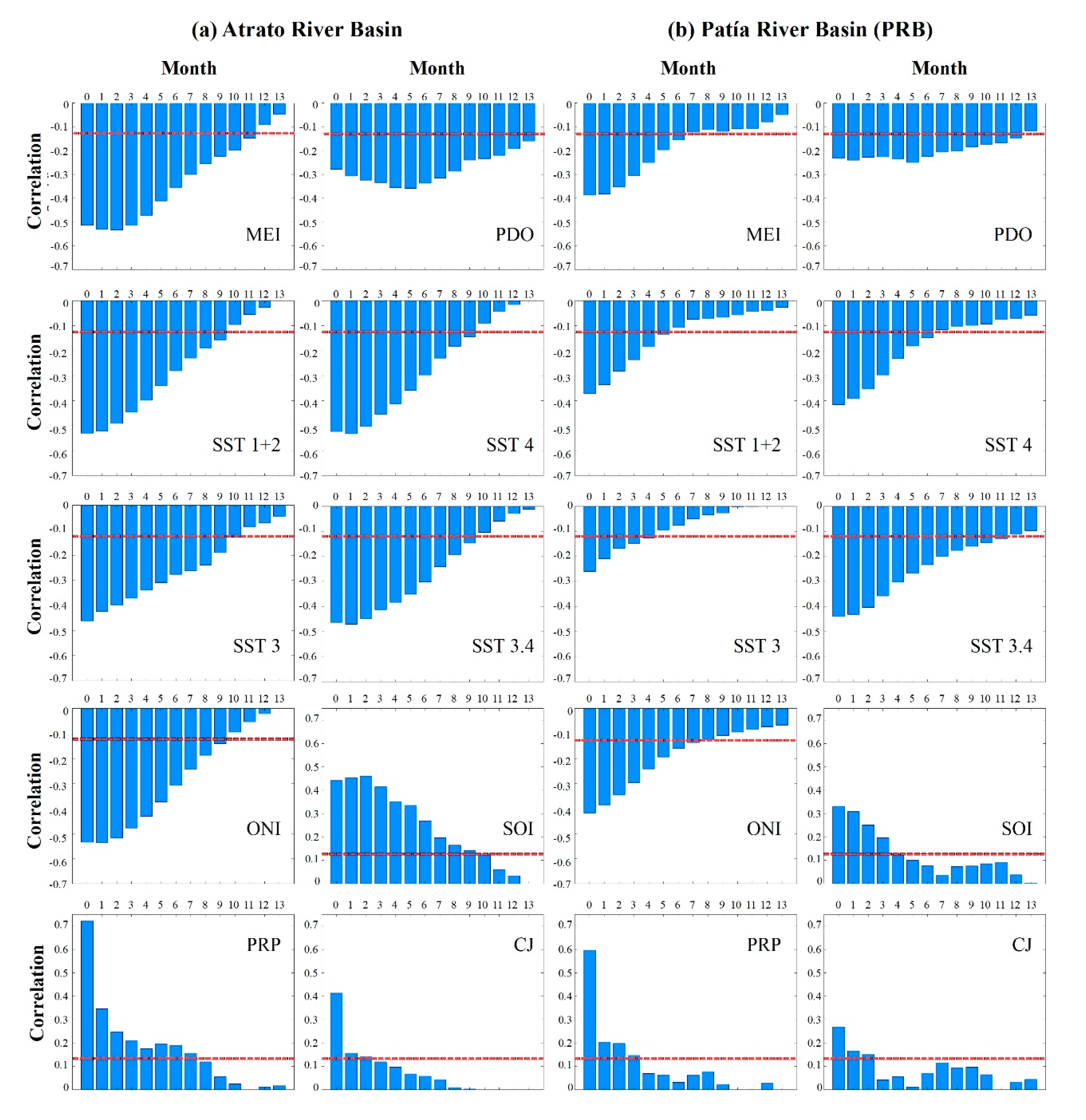
3.3. Kendall’s Tau Correlation and Cross-Correlation with Climate Indices

The influence of large-scale climate phenomena on the variability of the ARB and PRB hydrology was studied using correlation analysis. Figure 4 shows the correlation coefficients between the PC1s of both studied basins and the selected climate indices in lag 0. The monthly correlations for ARB showed statistically significant positive (negative) relations mainly with precipitation (PRP), CJ, and SOI (ONI, MEI, SST1+2 and SST4) (Figure 4a). For PRB (Figure 4b), the highest positive (negative) correlations statistically significant were presented with PRP, CJ, and SOI (ONI, MEI, SST3.4, and SST4). These results indicate that a direct (inverse) relation exists between the atmospheric (oceanic) variables and the streamflows of the ARB and PRB.

These results are consistent with those obtained by Carvajal et al. [56], Puertas and Carvajal [58], Poveda et al. [20], and Ávila et al. [57], who reported a reduction (increase) in the streamflows associated with the positive (negative) values of the oceanic ENSO-related indices. Poveda et al. [19] and Rueda and Poveda [89] also reported that a direct teleconnection existed between the streamflows of the rivers in western Colombia and the SOI and CJ indices. These findings are coherent with those presented herein. According to Poveda and Mesa [63], during EN events the CJ weakens strongly with the consequent reduction in rainfall while in LN events the CJ intensifies owing to the quantity of moisture that it transports which, in turn, interacts with easterly trade winds to result in high atmospheric instability and, consequently, in vast amounts of convection and rainfall.

The results in

Table 4. Kendall’s correlation between the annual, maximum, and minimum PC1s and climate indices. Statistically significant correlations at the 5% significance level are show in bold.

	PC1	ONI	MEI	SST1+2	SST3	SST3.4	SST4	PDO	SOI	PRP	CJ	TNA	NAO
ARB	Annual	−0.52	−0.45	−0.48	−0.40	−0.40	−0.49	−0.28	0.47	0.54	0.33	0.12	−0.08
	Maximum	−0.30	−0.25	−0.27	−0.20	−0.30	−0.32	−0.15	0.32	0.3	0.23	0.10	−0.10
	Minimum	−0.42	−0.39	−0.42	−0.39	−0.33	−0.40	−0.30	0.36	0.44	0.22	0.03	0.02
PRB	Annual	−0.35	−0.37	−0.36	−0.23	−0.32	−0.37	−0.25	0.29	0.55	0.22	−0.02	0.09
	Maximum	−0.40	−0.38	−0.34	−0.21	−0.37	−0.41	−0.23	0.35	0.57	0.31	0.09	−0.04
	Minimum	−0.11	−0.14	−0.19	−0.12	−0.11	−0.12	−0.05	0.03	0.27	0.03	−0.39	0.30

show significant negative (positive) correlations between the minimum PRB streamflows and TNA (NAO). This result shows that the PRB streamflows can be influenced by factors other than ENSO. This finding is coherent with Poveda and Mesa [60], who indicated a nonlinear dependence of Colombian hydroclimatology with NAO, and also with Carvajal et al. [56], who reported negative correlations between TNA and the streamflows of rivers that lie south of the Colombian Pacific.

The cross-correlation analysis with a lag of up to 12 months between the PC1s of the ARB and PRB and the climate indices revealed a significant persistence up to a delay of 9 months (Figure 5). Such persistence might be due to the linkages of the rainfall, temperature, evapotranspiration, soil moisture, and run-off in the hydrographic basins [18,90]. This result is coherent with that obtained by Navarro et al. [22], who reported persistence for up to 6, 7, 8, and 9 months for teleconnections between rainfall in stations in western Colombia and the oceanic ENSO-related indices. For the ARB, the highest correlation coefficients between streamflows and the climate indices for the following lags were 0 (SST1+2, SST3, PRP, and CJ), 1 (SST4, SST3.4, and ONI), 2 (MEI and SOI), and 5 (PDO) months. For PRB, the maximum correlation coefficient was recorded with a zero-lag for all the indices, except for PDO, with a 5-month lag. The cross-correlation in lag 0 estimated by Pearson was consistent with the relation shown through the Kendall correlation.

Simultaneous significant correlations were identified with atmospheric indices PRP and CJ (Figure 5). These indices are related to one another because as the CJ reaches the western mountain range of the Colombian Andes, it rises due to the orographic effect and interacts with the trade winds facilitating the rise of a vast quantity of moisture. It generates an accelerated process of deep convection [63], which causes positive rainfall and streamflow anomalies for the Pacific region. These results are also coherent with Serna et al. [53], who reported that CJ is related to SST in the eastern TPO, since the winds associated with the CJ present more variability during canonical EN events, which reduce the SST and pressure gradients between the eastern TPO and western Colombia due to a more pronounced heating in the eastern TPO.

Unlike the ARB, the maximum correlations were obtained for the PRB with all the ENSO-related ocean indices synchronously (i.e., with lag 0). In spatial terms, this indicates that the influence of the ENSO phenomenon on the streamflows in the Colombian South Pacific was more immediate than the influence recorded on the streamflows in the Colombian North Pacific. Nonetheless, the ENSO phenomenon influence was stronger on the ARB than on the PRB because the correlation coefficients between the indices and streamflows of the ARB were higher than the coefficients recorded for the PRB. This result reveals that the influence of the oceanic climate indices is stronger on the streamflows of the basin closer to the TPO. This finding agrees with Poveda et al. [19], who indicated that the relation between the SOI index and the monthly streamflows of 50 rivers in Colombia was stronger in the stations closer to the TPO.

Finally, statistically significant negative correlation coefficients between the PDO Index and the PC1s of both ARB and PRB were observed (Figure 4), with maximum values for a 5-month lag (Figure 5). According to Kayano and Andreoli [91], PDO can influence the frequency of ENSO events depending on the phase. Thus, the negative correlations with PDO and ENSO indicated that the occurrence of higher (lower) streamflows is favored while negative LN/PDO (positive EN/PDO) events occur.

The correlation analyses show that the ARB and PRB streamflows relate negatively with the ENSO indices and positively with SOI (Table 4). Previous studies have shown that under EN the tropical atmosphere features higher than normal SLP over Indonesia, below normal SLP over the central and eastern TPO, and an anomalous Walker circulation eastward displaced with anomalous upward movements over the eastern and central equatorial Pacific, where positive anomalies of SST prevail, and anomalous downward movements to the west and northern and northwestern South America [92,93,94]. In association to this anomalous Walker cell, low-level easterlies are established in the extreme eastern equatorial Pacific and adjacent areas including the ARB and PRB. Thus, the CJ is weakened, reducing the transport of moisture from the Pacific to northwestern South America. It is worth noting that the CJ index and the ARB and PRB streamflows are positively correlated (Table 4). Consequently, the rainfall and streamflow are reduced in the ARB and PRB. On the contrary, the LN presents the opposite anomaly patterns, as documented by Hoyos et al. [62,88] and Arias et al. [35].

Negative correlations between ARB and PRB with PDO indicate a positive teleconnection between ENSO and PDO. In this way, ENSO teleconnections for the streamflows and rainfall in the study basins are related to the PDO, which creates a background for these teleconnections that act constructively (destructively) when ENSO and PDO are in the same (opposite) phase, confirming the findings of Kayano and Andreoli [91] for South America.

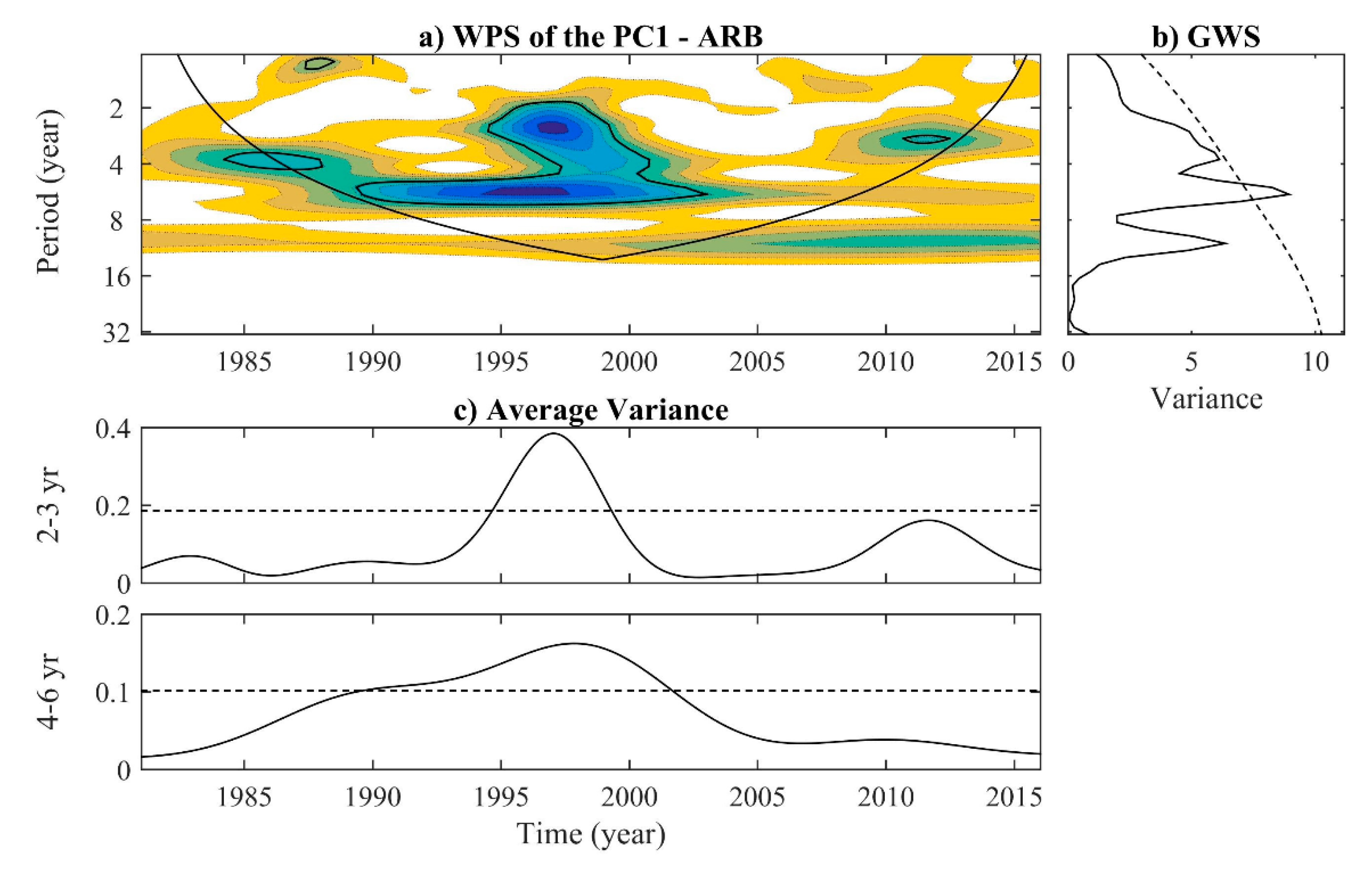
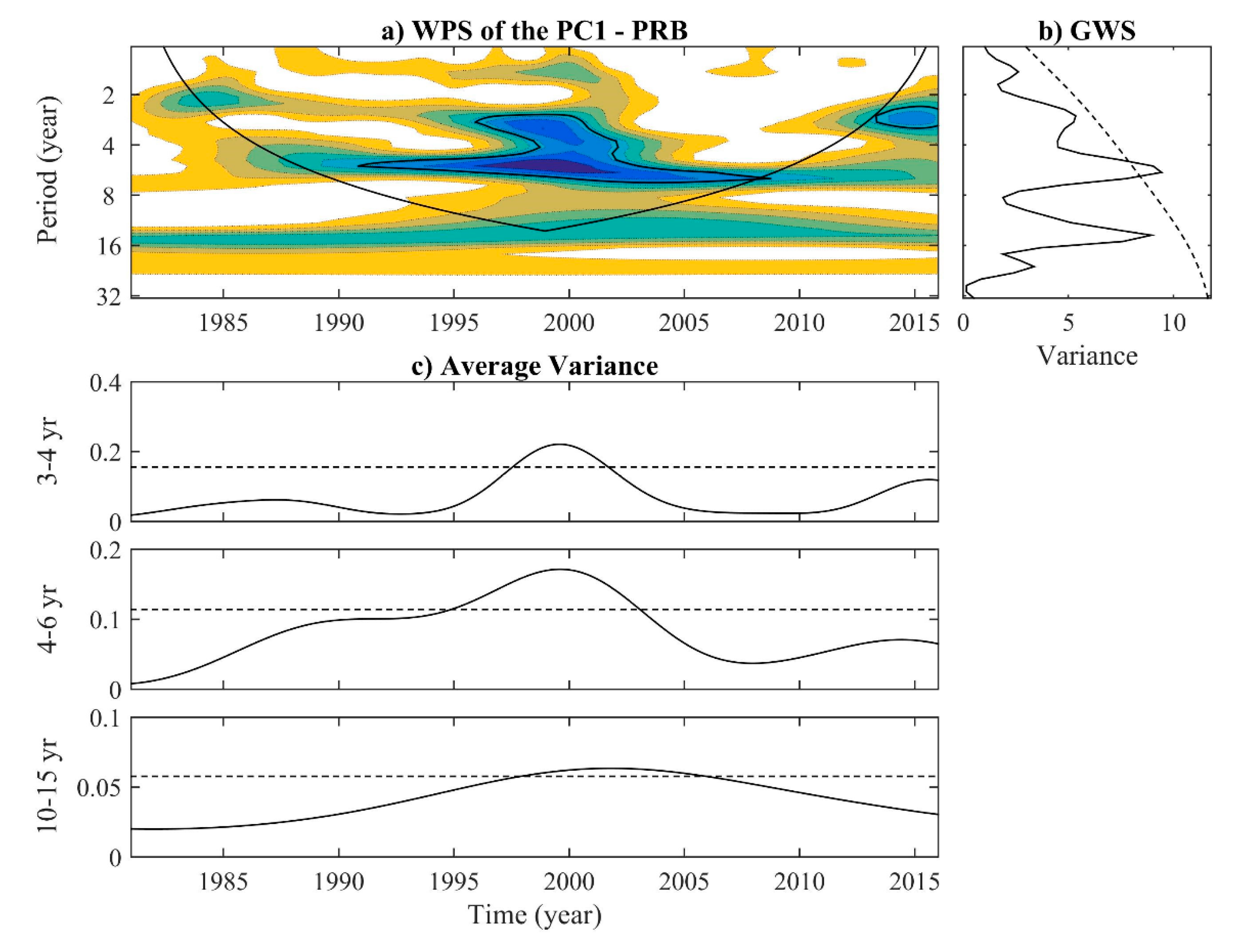
3.4. Wavelet Analysis

Both time and frequency variations were analyzed for the monthly PC1 of the ARB streamflows obtained by the wavelet transform. The energy spectrum showed a dominant variability on the 2–3-year and 4–6-year time scales owing to the significant variations (at the 5% level) during the 1995–2000 and 1990–2003 periods (Figure 6a). The energy spectrum of the PC for PRB showed a dominant and significant variability on the interannual 3–4-year and 4–6-year scales observed during the 1997–2003 and 1991–2009 periods (Figure 7a). Strong variability was found on the 10–15-year decadal scale owing to the nonsignificant variation during the 1997–2005 period (Figure 7a). The global wavelet spectrum (GWS) of the PC1s of both ARB and PRB are found in Figure 6b and Figure 7b, respectively. These figures indicate 4–6-year interannual peaks, which are significant at the 5% level for both basins. Nonsignificant peaks are seen on the 2–3- (3–4-) year interannual scale for ARB (PRB), and a peak on the 10–15-year decadal scale for PRB.

The scale-averaged wavelet power (SAP) scales were built for the 2–3- and 4–6-year scales for ARB, and for the 3–4-, 4–6-, and 10–15-year scales for PRB (Figure 6c and Figure 7c, respectively). The SAP was obtained from using Equation (24) described in Torrence and Compo [79], which allows to examine the scale modulations in the same time series [83]. In general, both basins show similar time fluctuations of the SAP (in variance units) series on the 4–6-year scale with significant values for ARB between 1990 and 2002 and for PRB between 1995 and 2004. For the ARB (PRB), the 2–3- (3–4-) year interannual scale showed significant values for the 1994–1999 (1997–2002) period. The SAP series for the 10–15-year scale for PRB presented almost significant values during the 1995–2010 period.

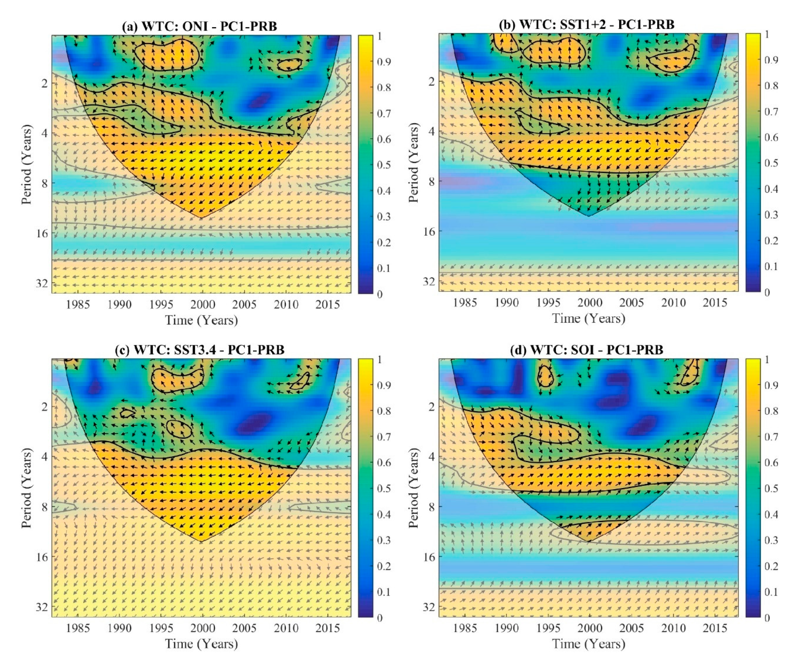
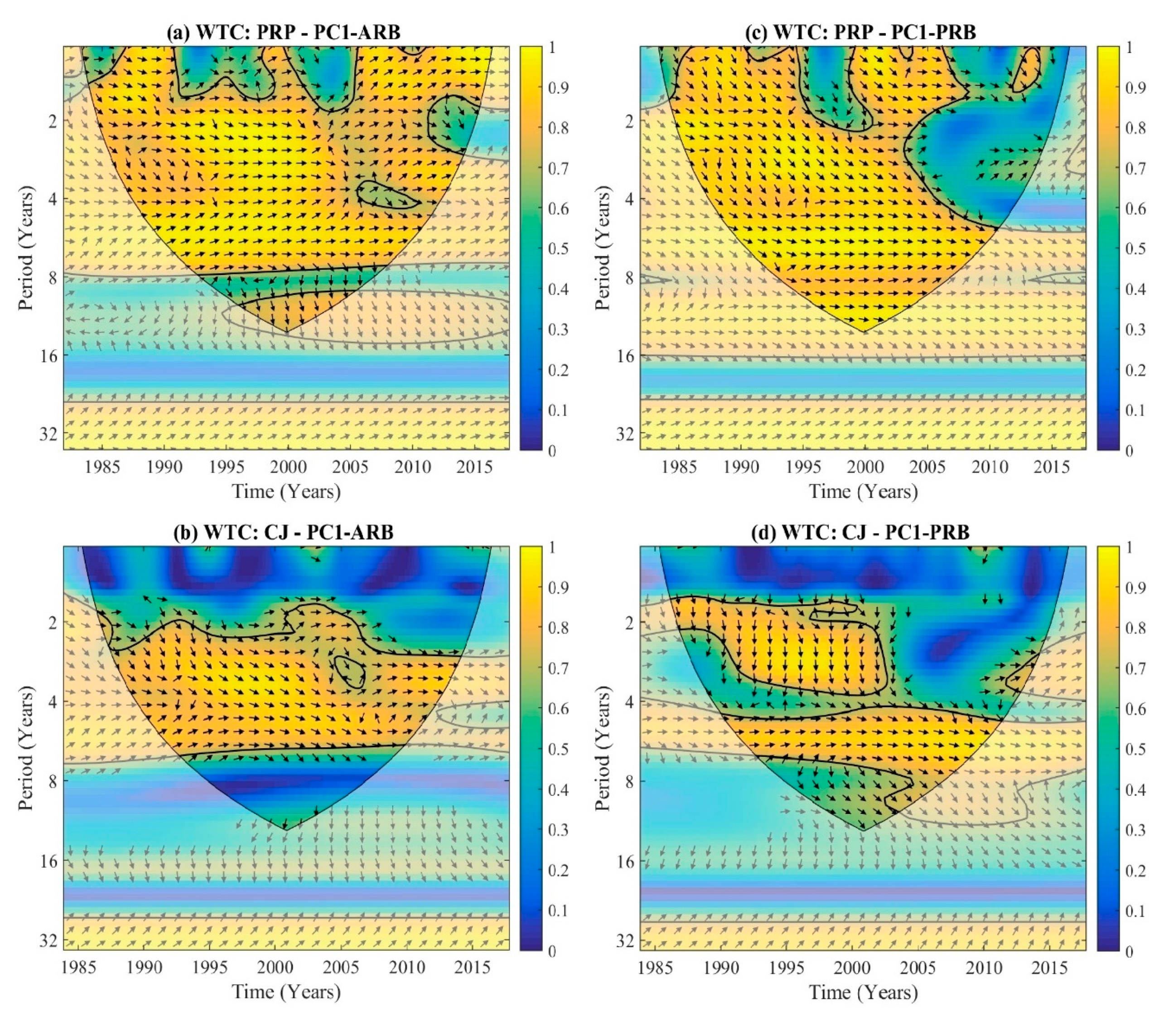
3.5. Wavelet Coherence and Phase Difference

The wavelet coherences between the PC1 for ARB and the ONI, MEI, SST1+2, and SST4 (SST3) indices led to similar relations, mainly on the 2–7-year time scale from 1990 to 2010 (1985 to 2017), with a phase difference from −160° to 180° (Figure 8a and

Table 5. Main results obtained by wavelet transform coherence.

Indices	ARB			PRB
	Scale		Lags (Months)	Scale		Lags (Months)
	Interannual	Decadal	Interannual/Decadal	Interannual	Decadal	Interannual/Decadal
ONI	2–7 years (-)	8–16 years (-)	0–5/5–9	4–8 years (-)	8–14 years (-)	0–5/5–9
MEI	2–7 years (-)	8–16 years (-)	0–5/5–9	2–7 years (-)	10–14 years (-)	0–7/
SST1+2	2–7 years (-)	8–12 years (-)	0–5/5–9	2–7 years (-)		0–7/
SST3	2–7 years (-)		0–5/	2–7 years (-)		0–7/
SST3.4	3–6 years (-)	10–12 years (-)	2–4/3–4	4–8 years (-)	8–14 years (-)	0/8–14
SST4	2–7 years (-)	10–14 years (-)	0–5/5–9	4–8 years (-)	8–14 years (-)	0–5/5–9
PDO				5–7 years (-)		2–7/
SOI	2–7 years (+)	10–14 years (+)	0–5/3–5	4–7 years (+)	10–12 years (+)	0–5/15–18
PRP	2–8 years (+)	10–14 years (+)	0–3/15–21	2–8 years (+)	8–14 years (+)	0–12/0–5
CJ	2–7 years (+)		3–11/	2–3 years and 4–6 years (+)		0–2 and 6–9/

(+) Phase, (-) Anti-phase.

). The −160° phase difference for the 2–7-year interannual scale indicates that dry (wet) conditions preceded the mature EN (LN) phase by approximately 1–5 months. The 180° phase difference means that the mature phase of the EN (LN) events occurred simultaneously with minimum (maximum) streamflows. These series also displayed considerable coherence on the 8–16-year decadal scale from 1995 to 2007 with a −160° phase difference, which indicates minimum (maximum) streamflows preceded the mature EN (LN) phase by approximately 5–9 months, except for SST3, for which no decadal coherence was observed (Figure 8b).

The relationship between El Niño 3.4 and PC1 for ARB was more reduced. Figure 8c shows significant coherence at an interannual scale (3–6 years) from 1988 to 2010 with a phase difference from −160° to 180°, and for the decadal-scale (10–12 years) from 1997 to 2007 with a phase difference of −170°. The phase difference from −160° to −170° indicates that the maximum (minimum) streamflow anomalies precede the minimum (maximum) variations in SST3.4 by 2–4 and 3–4 months for the interannual and decadal scales, respectively.

Significant coherences were observed with SOI on the 2–7-year interannual scale from 1987 to 2013, with phase differences from 0° to 20° (Figure 8d). A 20° phase difference indicates that the negative (positive) streamflow anomalies were followed by negative (positive) SOI values with a delay of approximately 1–5 months, whereas 0° suggests that both time series were simultaneously related. Coherence was observed on the 10–14-year decadal scale from 1995 to 2005 with a phase difference from 0° to 10°, indicating that a decrease (increase) in streamflow precedes a low (high) pressure in the eastern TPO by approximately 3–5 months.

The coherence analyses between the PC1 of the PRB and the indices gave similar results for the ONI and SST4, mainly on the 4–8-year time scale from 1987 to 2011, with a phase difference from −160° to 180°, establishing a phase difference around 2–5 months between minimum peak of streamflow and the maximum peak of the indices. Coherences were found on the 8–14-year decadal scale from 1994 to 2007, with a −160° phase difference, which indicates that the anomalies of the streamflow in PRB precede the variations in the SST4 by about 5–9 months (Figure 9a). The 180° phase difference indicates simultaneous alterations.

Figure 9b also shows significant relations on the 2–7-year interannual time scale from 1986 to 2013, with a phase difference from −150° to 180°. For this time scale, the phase difference of −150° generates a lag between the maximum peak of the indices and the minimum peak of the streamflow of 30° (2–7 months). In other words, the maximum (minimum) streamflow anomalies occur in the development phase of an LN (EN) event. Simultaneous variations were also observed between SST anomalies in the Niño 3.4 region and PRB streamflow on the 4–8-year time scale from 1986 to 2011 (Figure 9c). The relation between SOI and the PRB streamflow can be seen in Figure 9d. One link was found, mainly during the 1990–2010 period, with a phase difference from 0° to 20° on the 4–7-year scale indicating 3–5-month lags. These series also showed coherence on the 10–12-year time scale for the 1996–2004 period, with a 45° phase difference, that means lags of approximately 15–18 months (Figure 9d).

Therefore, the present work reveals that the SST anomalies in different ENSO regions cause distinct ARB and PRB streamflow responses, whose temporal persistence also varies. This could be due to the orographical diversity in West Colombia [26,95], and also to the influence of different atmospheric factors, which indicate considerable complexity in the spatiotemporal structure of precipitation and other hydroclimate variables in the region [96].

The coherence between the PC1 for ARB (PRB) and PRP was significant on the 2–8-year time scale from 1985 to 2011 with a phase difference from 0° to 10° (0° to 45°) (Figure 10a,c). For this scale, the 10° (45°) difference indicated that the influence of PRP on streamflows was recorded with 1–3 (3–12) month lags, whereas 0° indicated that both time series were simultaneously related. On the 10–14 (8–14) year decadal scale, the indices presented −45° (0° and 10°) phase difference, which implies that the influence of PRP on streamflows of ARB (PRB) was reflected within a 15–21 (3–5) month time interval.

The CJ index and PC1 for ARB showed coherences on the 2–7-year interannual scale from 1988 to 2013 (Figure 10b), with phase differences from 0 to −45°, meaning a delay of approximately 3–11 months. Significant coherences between the CJ and PC1 for PRB were observed on two interannual scales (Figure 10d): (i) from 1987 to 2003 on the 2–3-year scale, with a −90° phase difference, which indicates a time of 6–9 months beforehand between the CJ index and the basin streamflows, and (ii) from 1990 to 2011 on the 4–6-year scale, with phase differences from 0° to −10°, indicating lags of 1–2 months between the CJ index and the PRB streamflows.

The influence that CJ has on both basins’ streamflow anomalies has been previously documented and is relevant for the vast quantities of moisture being transported toward the continent, which would explain why Colombia is considered one of the rainiest areas in the world [28]. Poveda and Mesa [52,63] reported an average moisture transport rate close to 3.78 × 106 kg·s⁻¹ or 3774 m³·s⁻¹, which would directly contribute to the annual discharge of ≈5000 m³·s⁻¹ for the ARB and San Juan River, and is one of the highest run-off rates worldwide. The wavelet coherences analyses with CJ index identified different responses of streamflows such that the anomalous moisture transport associated with CJ responds more immediately to the PRB streamflow anomalies (0–9 months) compared to ARB (3–11 months).

The coherence results obtained with PDO are depicted in Table 5. It was not possible to define a significant coherence with the ARB streamflows, and the relation with PRB was observed during the 1987–2011 period on the 5–7-year scale, with a phase difference from −170° to −150° that generates a lag between the maximum of the PDO index and the minimum peak of streamflows by 2–7 months beforehand (figure not shown).

4. Conclusions

The climate variability is a factor that affects the water resources in Colombia, which presents a spatiotemporal variability linked to the physiology of basins and the climatic features of the region. The present research estimated the main variability time scales of the streamflow of the Atrato River Basin (ARB) and Patía River Basin (PRB) of the Colombian Pacific region, and their relations to the large-scale climate variability.

The estimation of the missing data from the ARB and PRB using the nonlinear principal component analysis (NLPCA) methodology gave an RRMSE of 0.03 and 0.39, respectively. The better estimation of the missing values for the ARB, compared to the PRB, result from the lower coefficients of variation for the gauges compared to the PRB, as well as the reduced number of missing data points. Furthermore, these results indicate that the NLPCA approach is a powerful alternative in the estimation of streamflow missing data since it uses nonlinear and nonstationary features of the data.

The PCA allowed to represent the variability modes of the streamflows for the ARB and PRB. These temporal series were useful to analyze the connections between climate indices and streamflows. The first variability modes in the ARB and PRB streamflows showed coincidences on the positive (negative) values for the 1988–1989, 1998–1999, and 2010–2011 (1997–1998 and 2015–2016) periods which coincided with La Niña-LN (El Niño-EN) events.

The correlations analyses between the PC1s of the streamflows of the ARB and PRB and the climate indices indicate their primary relations. The significant positive (negative) high correlations with the atmospheric (oceanic) indices indicates a direct relation with the PRP, CJ, and SOI indices and an inverse one with the ONI and MEI indices, and SST indices for the TPO. The magnitudes of the correlation coefficients indicated a stronger influence for the climate indices on the ARB than on the PRB. However, the influence on the PRB was more immediate than that on the ARB. Conversely, the indices related to the NAO did not impact the modulation of the variability for the monthly and annual streamflows of both studied basins.

The cross-correlation and wavelet coherence analyses revealed that the variability of the ARB (PRB) streamflows was influenced mainly by the SST1+2 and SST4 (SST3.4 and SST4) anomalies on the 2–7- (4–8-) year interannual scale and on the 8–12- (8–14-) year decadal scale. These results imply that the SST anomalies in different ENSO regions cause distinct responses in the ARB and PRB streamflows, with distinct temporal persistence. For the ARB, in the interannual (2–7 years) and decadal (8–14 years) scales, the relations are preferably associated with the SST in the east and west TPO (indices SST1+2, SST4, ONI, and MEI) with maximum (minimum) streamflow anomalies occurring up to 0–5 (5–9) months in advance and simultaneously with the minimum (maximum) SST indices. For the PRB, the relations are preferably with the SST in the central and western regions of the TPO (indices SST3.4, SST4 and ONI), in the interannual (4–8 years) and decadal (8–14 years) scale, and the decreases (increases) in streamflow precede the EN (LN) mature stage by approximately 0–5 (5–9) months.

The most relevant contribution of the present research is the multiscale relations between the streamflows of both basins in the Colombian Pacific and the SST, which previous works have not documented and that allow an understanding mainly of the influence of oceanic climate indices linked to the TPO. Through this study, we understand that the EN tends to reduce the rainfall and river levels, rising the probabilities of drought over ARB and PRB, whereas, the LN increases rainfall, river levels, and the likelihood of flooding. Therefore, if we knew that the warm (cold) phase of a climate anomaly such as ENSO will be active, we can generally expect that ARB and PRB will have dry (rainy) weather periods. Hence, these results are useful for the management, planning, and implementing action plans for the sustainable use of water resources in these basins.

Finally, the results herein obtained are expected to contribute to long-term hydrological forecasts in the ARB and PRB to enable the estimates made on the future state of these water systems to be more accurately evaluated in climate variability scenarios. One of the most important aspects of research relates to possible impacts associated with global warming. However, this issue is outside the scope of this study, and future studies are needed to evaluate possible changes. To this end, climate modeling studies can address these aspects, separating the components of global change and natural variability, and deepening the impact on the basins involved in addition to changes in land use.

References

1. Coulibaly, P. Spatial and temporal variability of Canadian seasonal precipitation (1900–2000). Adv. Water Resour. 2006, 29, 1846–1865. [Google Scholar] [CrossRef]
2. Jiang, R.; Gan, T.Y.; Xie, J.; Wang, N. Spatiotemporal variability of Alberta’s seasonal precipitation, their teleconnection with large-scale climate anomalies and sea surface temperature. Int. J. Climatol. 2014, 34, 2899–2917. [Google Scholar] [CrossRef]
3. Pasquini, A.I.; Depetris, P.J. Discharge trends and flow dynamics of South American rivers draining the southern Atlantic seaboard: An overview. J. Hydrol. 2007, 333, 385–399. [Google Scholar] [CrossRef]
4. Coulibaly, P.; Burn, D.H. Wavelet analysis of variability in annual Canadian streamflows. Water Resour. Res. 2004, 40. [Google Scholar] [CrossRef]
5. Capozzoli, C.R.; Cardoso, A.d.O.; Ferraz, S.E.T. River flow variability patterns in Main Brazilian basins and association with climate indices. Revista Brasileira de Meteorologia 2017, 32, 243–254. [Google Scholar] [CrossRef] [Green Version]
6. Eltahir, E.A. El Niño and the natural variability in the flow of the Nile River. Water Resour. Res. 1996, 32, 131–137. [Google Scholar] [CrossRef]
7. Siam, M.S.; Eltahir, E.A. Explaining and forecasting interannual variability in the flow of the Nile River. Hydrol. Earth Syst. Sci. 2015, 19, 1181–1192. [Google Scholar] [CrossRef] [Green Version]
8. Sagarika, S.; Kalra, A.; Ahmad, S. Interconnections between oceanic–atmospheric indices and variability in the US streamflow. J. Hydrol. 2015, 525, 724–736. [Google Scholar] [CrossRef]
9. Tamaddun, K.A.; Kalra, A.; Bernardez, M.; Ahmad, S. Multi-scale correlation between the western US snow water equivalent and ENSO/PDO using wavelet analyses. Water Resour. Manag. 2017, 31, 2745–2759. [Google Scholar] [CrossRef]
10. Konapala, G.; Veettil, A.V.; Mishra, A.K. Teleconnection between low flows and large-scale climate indices in Texas River basins. Stoch. Environ. Res. Risk Assess. 2018, 32, 2337–2350. [Google Scholar] [CrossRef]
11. Tamaddun, K.A.; Kalra, A.; Ahmad, S. Spatiotemporal Variation in the Continental US Streamflow in Association with Large-Scale Climate Signals Across Multiple Spectral Bands. Water Resour. Manag. 2019, 33, 1–22. [Google Scholar] [CrossRef]
12. Handorf, D.; Dethloff, K. Atmospheric teleconnections and flow regimes under future climate projections. Eur. Phys. J. Spec. Top. 2009, 174, 237–255. [Google Scholar] [CrossRef]
13. Mihaila, D.; Briciu, A.-E. Climatic teleconnections with influence on some rivers from south-eastern Europe. Boletin de la Asociacion de Geografos Espanoles 2015, 69, 37–62. [Google Scholar]
14. Rodríguez Fonseca, B.; Casado Calle, M.J.; Barriopedro, D. Modes of Variability Affecting Southwestern Europe. CLIVAR Exchanges 2017, 73, 24–31. [Google Scholar]
15. Kim, J.S.; Jain, S.; Yoon, S.K. Warm season streamflow variability in the Korean Han River Basin: Links with atmospheric teleconnections. Int. J. Climatol. 2012, 32, 635–640. [Google Scholar] [CrossRef]
16. Yoon, S.; Lee, T. Investigation of hydrological variability in the Korean Peninsula with the ENSO teleconnections. Proc. Int. Assoc. Hydrol. Sci. 2016, 374, 165–173. [Google Scholar] [CrossRef] [Green Version]
17. Mechoso, C.R.; Iribarren, G.P. Streamflow in southeastern South America and the southern oscillation. J. Clim. 1992, 5, 1535–1539. [Google Scholar] [CrossRef]
18. Poveda, G.; Mesa, O.J. Feedbacks between hydrological processes in tropical South America and large-scale ocean–atmospheric phenomena. J. Clim. 1997, 10, 2690–2702. [Google Scholar] [CrossRef]
19. Poveda, G.; Gil, M.M.; Quiceno, N. El ciclo anual de la hidrología de Colombia en relación con el ENSO y la NAO. Bulletin de l’Institut Français d’études Andines 1998, 27, 721–731. [Google Scholar]
20. Poveda, G.; Álvarez, D.M.; Rueda, Ó.A. Hydro-climatic variability over the Andes of Colombia associated with ENSO: A review of climatic processes and their impact on one of the Earth’s most important biodiversity hotspots. Clim. Dyn. 2011, 36, 2233–2249. [Google Scholar] [CrossRef]
21. Enciso, A.M.; Carvajal-Escobar, Y.; Sandoval, M.C. Hydrological analysis of historical floods in the upper valley of Cauca river: Análisis hidrológico de las crecientes históricas del río Cauca en su valle alto. Ingeniería y Competitividad 2016, 18, 47–58. [Google Scholar]
22. Navarro, E.; Vieira, C.; Arias, P. Spatiotemporal variability of the precipitation in Colombia during ENSO events. XV Seminario Iberoamericano de Redes de Agua y Drenaje SEREA2017 2017, 1, 1–8. [Google Scholar]
23. Ávila, Á.; Guerrero, F.C.; Escobar, Y.C.; Justino, F. Recent Precipitation Trends and Floods in the Colombian Andes. Water 2019, 11, 379. [Google Scholar] [CrossRef] [Green Version]
24. Navarro, E.; Arias, P.A.; Vieira, S.C. El Niño-Oscilación del Sur, fase Modoki, y sus efectos en la variabilidad espacio-temporal de la precipitación en Colombia. Revista de la Academia Colombiana de Ciencias Exactas Físicas y Naturales 2019, 43, 120–132. [Google Scholar] [CrossRef]
25. Loaiza Cerón, W.; Toshie Kayano, M.; Andreoli, R.V.; Avila, A.; Canchala, T.; Francés, F.; Ayes Rivera, I.; Alfonso-Morales, W.; Ferreira de Souza, R.A.; Carvajal-Escobar, Y. Streamflow Intensification Driven by the Atlantic Multidecadal Oscillation (AMO) in the Atrato River Basin, Northwestern Colombia. Water 2020, 12, 216. [Google Scholar] [CrossRef] [Green Version]
26. Poveda, G. La hidroclimatología de Colombia: Una síntesis desde la escala inter-decadal hasta la escala diurna. Rev. Acad. Colomb. Cienc 2004, 28, 201–222. [Google Scholar]
27. Hurtado, M.A.F.; Mesa, S.Ó.J. Reconstrucción de los campos de precipitación mensual en Colombia. Escuela de Geociencias y Medio Ambiente 2014, 81, 251–258. [Google Scholar]
28. Poveda, G.; Jaramillo, L.; Vallejo, L.F. Seasonal precipitation patterns along pathways of South American low-level jets and aerial rivers. Water Resour. Res. 2014, 50, 98–118. [Google Scholar] [CrossRef]
29. Mittermeier, R.A.; Turner, W.R.; Larsen, F.W.; Brooks, T.M.; Gascon, C. Global biodiversity conservation: The critical role of hotspots. In Biodiversity Hotspots; Springer: Berlin/Heidelberg, Germany, 2011; pp. 3–22. [Google Scholar]
30. Velásquez-Restrepo, M.; Poveda, G. Estimación del balance hídrico de la región Pacífica Colombiana. DYNA 2019, 86, 297–306. [Google Scholar] [CrossRef]
31. Montealegre, E.J.; Pabón, J.D. La variabilidad climática interanual asociada al ciclo El Niño-La Niña-Oscilación del Sur y su efecto en el patrón pluviométrico de Colombia. Meteorología Colombiana 2000, 2, 7–21. [Google Scholar]
32. Tedeschi, R.G.; Cavalcanti, I.F.; Grimm, A.M. Influences of two types of ENSO on South American precipitation. Int. J. Climatol. 2013, 33, 1382–1400. [Google Scholar] [CrossRef]
33. Tedeschi, R.G.; Grimm, A.M.; Cavalcanti, I.F. Influence of Central and East ENSO on extreme events of precipitation in South America during austral spring and summer. Int. J. Climatol. 2015, 35, 2045–2064. [Google Scholar] [CrossRef]
34. Loaiza, W.; Carvajal-Escobar, Y.; Andreoli, R.V.; Kayano, M.T.; Gonzáles, N. Spatio-temporal varibility of the droughts in Cali, Colombia and their relationships with the El Niño-Southern Oscillation (ENSO) between 1971 and 2011. Atmósfera 2020, 33, 51–69. [Google Scholar] [CrossRef]
35. Arias, P.A.; Martínez, J.A.; Vieira, S.C. Moisture sources to the 2010–2012 anomalous wet season in northern South America. Clim. Dyn. 2015, 45, 2861–2884. [Google Scholar] [CrossRef]
36. Hoyos, I.; Dominguez, F.; Cañón-Barriga, J.; Martínez, J.; Nieto, R.; Gimeno, L.; Dirmeyer, P. Moisture origin and transport processes in Colombia, northern South America. Clim. Dyn. 2018, 50, 971–990. [Google Scholar] [CrossRef]
37. Jaramillo, L.; Poveda, G.; Mejía, J.F. Mesoscale convective systems and other precipitation features over the tropical Americas and surrounding seas as seen by TRMM. Int. J. Climatol. 2017, 37, 380–397. [Google Scholar] [CrossRef]
38. Bedoya-Soto, J.; Aristizabal, E.; Carmona, A.M.; Poveda, G. Seasonal Shift of the Diurnal Cycle of Rainfall Over Medellin’s Valley, Central Andes of Colombia (1998–2005). Front. Earth Sci. 2019, 7, 92. [Google Scholar] [CrossRef]
39. Poveda, G.; Vélez, J.; Mesa, O.; Hoyos, C.; Mejía, J.F.; Barco, O.J.; Correa, P.L. Influencia de fenómenos macroclimáticos sobre el ciclo anual de la hidrología colombiana: Cuantificación lineal, no lineal y percentiles probabilísticos. Meteorología Colombiana 2002, 6, 121–130. [Google Scholar]
40. Cadavid, J.M.; Salazar, J.E. Generación de series sinteticas de caudales usando un Modelo Matalas con medias condicionadas. Avances en Recursos Hidráulicos 2008, 17, 17–24. [Google Scholar]
41. Tootle, G.A.; Piechota, T.C.; Gutiérrez, F. The relationships between Pacific and Atlantic Ocean sea surface temperatures and Colombian streamflow variability. J. Hydrol. 2008, 349, 268–276. [Google Scholar] [CrossRef]
42. Rojo, J.D.; Carvajal, L.F. Predicción no lineal de caudales utilizando variables macroclimáticas y análisis espectral singular. Tecnología y Ciencias del Agua 2010, 1, 59–73. [Google Scholar]
43. Rodríguez-Rubio, E. A multivariate climate index for the western coast of Colombia. Adv. Geosci. 2013, 33, 21–26. [Google Scholar] [CrossRef] [Green Version]
44. Córdoba-Machado, S.; Palomino-Lemus, R.; Gámiz-Fortis, S.R.; Castro-Díez, Y.; Esteban-Parra, M.J. Influence of tropical Pacific SST on seasonal precipitation in Colombia: Prediction using El Niño and El Niño Modoki. Clim. Dyn. 2015, 44, 1293–1310. [Google Scholar] [CrossRef]
45. Cuadrado, P.B.; Blanco, R.J. Teleconexiones y eventos extremos de sequía en áreas protegidas del norte de Colombia. Revista de Climatología 2015, 15, 27–38. [Google Scholar]
46. Rodríguez-Fonseca, B.; Polo, I.; García-Serrano, J.; Losada, T.; Mohino, E.; Mechoso, C.R.; Kucharski, F. Are Atlantic Niños enhancing Pacific ENSO events in recent decades? Geophys. Res. Lett. 2009, 36. [Google Scholar] [CrossRef]
47. Mosquera-Machado, S.; Ahmad, S. Flood hazard assessment of Atrato River in Colombia. Water Resour. Manag. 2007, 21, 591–609. [Google Scholar] [CrossRef]
48. Wolter, K.; Timlin, M.S. El Niño/Southern Oscillation behaviour since 1871 as diagnosed in an extended multivariate ENSO index (MEI. ext). Int. J. Climatol. 2011, 31, 1074–1087. [Google Scholar] [CrossRef]
49. L’Heureux, M.L.; Collins, D.C.; Hu, Z.-Z. Linear trends in sea surface temperature of the tropical Pacific Ocean and implications for the El Niño-Southern Oscillation. Clim. Dyn. 2013, 40, 1223–1236. [Google Scholar] [CrossRef] [Green Version]
50. Mantua, N.J.; Hare, S.R.; Zhang, Y.; Wallace, J.M.; Francis, R.C. A Pacific interdecadal climate oscillation with impacts on salmon production. Bull. Am. Meteorol. Soc. 1997, 78, 1069–1080. [Google Scholar] [CrossRef]
51. Hurrel, J.W.; Kushnir, Y.; Ottersen, G.; Visbeck, M. The North Atlantic oscillation: Climatic significance and environmental impact. Geophys. Monogr. 2003, 134. [Google Scholar] [CrossRef]
52. Poveda, G.; Mesa, O.J. On the existence of Lloró (the rainiest locality on Earth): Enhanced ocean-land-atmosphere interaction by a low-level jet. Geophys. Res. Lett. 2000, 27, 1675–1678. [Google Scholar] [CrossRef] [Green Version]
53. Serna, L.M.; Arias, P.A.; Vieira, S.C. Las corrientes superficiales de chorro del Chocó y el Caribe durante los eventos de El Niño y El Niño Modoki. Revista de la Academia Colombiana de Ciencias Exactas Físicas y Naturales 2018, 42, 410–421. [Google Scholar] [CrossRef]
54. Dee, D.P.; Uppala, S.M.; Simmons, A.; Berrisford, P.; Poli, P.; Kobayashi, S.; Andrae, U.; Balmaseda, M.; Balsamo, G.; Bauer, D.P. The ERA-Interim reanalysis: Configuration and performance of the data assimilation system. Q. J. R. Meteorol. Soc. 2011, 137, 553–597. [Google Scholar] [CrossRef]
55. Funk, C.; Peterson, P.; Landsfeld, M.; Pedreros, D.; Verdin, J.; Shukla, S.; Husak, G.; Rowland, J.; Harrison, L.; Hoell, A. The climate hazards infrared precipitation with stations—A new environmental record for monitoring extremes. Sci. Data 2015, 2, 150066. [Google Scholar] [CrossRef] [PubMed] [Green Version]
56. Carvajal, Y.; Grisales, C.; Mateus, J. Correlación de variables macroclimáticas del Océano Pacífico con los caudales en los ríos interandinos del Valle del Cauca (Colombia). Revista Peruana de Biología 1999, 6, 9–17. [Google Scholar] [CrossRef] [Green Version]
57. Díaz, Á.J.Á.; Escobar, Y.C.; Serna, S.E.G. Análisis de la influencia de El Niño y La Niña en la oferta hídrica mensual de la cuenca del río Cali. Tecnura 2013, 18, 120–133. [Google Scholar]
58. Puertas; Carvajal. Incidence of El Niño southern oscillation in the precipitation and the temperature of the air in Colombia, using Climate Explorer. Ingeniería y Desarrollo 2008, 23, 104–118. [Google Scholar]
59. Tootle, G.A.; Piechota, T.C. Relationships between Pacific and Atlantic ocean sea surface temperatures and US streamflow variability. Water Resour. Res. 2008, 42. [Google Scholar] [CrossRef] [Green Version]
60. Poveda, G.; Mesa, O. La Oscilación del Atlántico Norte y su influencia sobre el clima de Colombia. In Proceedings of the Memorias XVII Congreso Latino-Americano de Hidráulica e Hidrología, IAHR, Guayaquil, Ecuador, 21 October 1996; pp. 343–354. [Google Scholar]
61. Hurtado, A. Estimación de los campos mensuales históricos de precipitación en el territorio colombiano. MSc Thesis, Posgrado en Aprovechamiento de Recursos Hidráulicos, Facultad de Minas, Universidad Nacional de Colombia sede Medellín, Colombia, 2009; pp. 1–104. [Google Scholar]
62. Hoyos, I.; Baquero-Bernal, A.; Jacob, D.; Rodríguez, B.A. Variability of extreme events in the Colombian Pacific and Caribbean catchment basins. Clim. Dyn. 2013, 40, 1985–2003. [Google Scholar] [CrossRef]
63. Poveda, G.; Mesa, O. La corriente de chorro superficial del Oeste (“del Chocó”) y otras dos corrientes de chorro en Colombia: Climatología y variabilidad durante las fases del ENSO”. Revista Académica Colombiana de Ciencia 1999, 23, 517–528. [Google Scholar]
64. Sierra, J.P.; Arias, P.A.; Vieira, S.C. Precipitation over northern South America and its seasonal variability as simulated by the CMIP5 models. Adv. Meteorol. 2015, 2015. [Google Scholar] [CrossRef] [Green Version]
65. Durán-Quesada, A.; Reboita, M.; Gimeno, L. Precipitation in tropical America and the associated sources of moisture: A short review. Hydrolo. Sci. J. 2012, 57, 612–624. [Google Scholar] [CrossRef]
66. Scholz, M.; Kaplan, F.; Guy, C.L.; Kopka, J.; Selbig, J. Non-linear PCA: A missing data approach. Bioinformatics 2005, 21, 3887–3895. [Google Scholar] [CrossRef] [Green Version]
67. Miró, J.J.; Caselles, V.; Estrela, M.J. Multiple imputation of rainfall missing data in the Iberian Mediterranean context. Atmos. Res. 2017, 197, 313–330. [Google Scholar] [CrossRef]
68. Canchala, T.; Carvajal-Escobar, Y.; Alfonso-Morales, W.; Loaiza, W.; Caicedo, E. Estimation of missing data of monthly rainfall in southwestern Colombia using artificial neural networks. Data Brief. 2019, 104517. [Google Scholar] [CrossRef]
69. Scholz, M.; Fraunholz, M.; Selbig, J. Nonlinear principal component analysis: Neural network models and applications. In Principal Manifolds for Data Visualization and Dimension Reduction; Springer: Berlin/Heidelberg, Germany, 2008; pp. 44–67. [Google Scholar]
70. Rousi, Ε.; Anagnostopoulou, C.; Tolika, K.; Maheras, P. Representing teleconnection patterns over Europe: A comparison of SOM and PCA methods. Atmos. Res. 2015, 152, 123–137. [Google Scholar] [CrossRef]
71. Tošić, I.; Zorn, M.; Ortar, J.; Unkašević, M.; Gavrilov, M.B.; Marković, S.B. Annual and seasonal variability of precipitation and temperatures in Slovenia from 1961 to 2011. Atmos. Res. 2016, 168, 220–233. [Google Scholar] [CrossRef]
72. Jolliffe, I.T.; Cadima, J. Principal component analysis: A review and recent developments. Phil. Trans. R. Soc. A 2016, 374, 20150202. [Google Scholar] [CrossRef]
73. Helena, B.; Pardo, R.; Vega, M.; Barrado, E.; Fernandez, J.M.; Fernandez, L. Temporal evolution of groundwater composition in an alluvial aquifer (Pisuerga River, Spain) by principal component analysis. Water Res. 2000, 34, 807–816. [Google Scholar] [CrossRef]
74. Jolliffe, I. Principal Component Analysis; Springer: New York, NY, USA, 1986; Volume 271, pp. 129–155. [Google Scholar]
75. Preisendorfer, R. Principal Component Analysis in Meteorology and Oceanography; Elsevier Science Publisher: Amsterdam, The Netherlands, 1988; Volume 17, p. 425. [Google Scholar]
76. Carvajal, Y.; Segura, J.B.M. Análisis de variabilidad de datos medioambientales aplicando funciones ortogonales empíricas o componentes principales. Ingeniería de Recursos Naturales y del Ambiente 2004, 1, 4–11. [Google Scholar]
77. Knight, W.R. A computer method for calculating Kendall’s tau with ungrouped data. J. Am. Stat. Assoc. 1966, 61, 436–439. [Google Scholar] [CrossRef]
78. Banimahd, S.A.; Khalili, D. Factors influencing Markov chains predictability characteristics, utilizing SPI, RDI, EDI and SPEI drought indices in different climatic zones. Water Resour. Manag. 2013, 27, 3911–3928. [Google Scholar]
79. Torrence, C.; Compo, G.P. A practical guide to wavelet analysis. Bull. Am. Meteorol. Soc. 1998, 79, 61–78. [Google Scholar] [CrossRef] [Green Version]
80. Labat, D. Wavelet analysis of the annual discharge records of the world’s largest rivers. Adv. Water Resour. 2008, 31, 109–117. [Google Scholar] [CrossRef]
81. Schulte, J.A.; Najjar, R.G.; Li, M. The influence of climate modes on streamflow in the Mid-Atlantic region of the United States. J. Hydrol. Reg. Stud. 2016, 5, 80–99. [Google Scholar] [CrossRef] [Green Version]
82. Tan, X.; Gan, T.Y.; Shao, D. Wavelet analysis of precipitation extremes over Canadian ecoregions and teleconnections to large-scale climate anomalies. J. Geophys. Res. Atmos. 2016, 121. [Google Scholar] [CrossRef]
83. Andreoli, R.V.; Kayano, M.T. Multi-scale variability of the sea surface temperature in the Tropical Atlantic. J. Geophys. Res. Oceans 2004, 109. [Google Scholar] [CrossRef] [Green Version]
84. Grinsted, A.; Moore, J.C.; Jevrejeva, S. Application of the cross wavelet transform and wavelet coherence to geophysical time series. Nonlinear Proc. Geophys. 2004, 11, 561–566. [Google Scholar] [CrossRef]
85. Torrence, C.; Webster, P.J. Interdecadal changes in the ENSO–monsoon system. J. Clim. 1999, 12, 2679–2690. [Google Scholar] [CrossRef] [Green Version]
86. Diaz, L.G.; Morales, M.A. Estadística Multivariada: Inferencia y Métodos; Universidad Nacional de Colombia: Bogota, Colombia, 2002. [Google Scholar]
87. Trenberth, K. The climate data guide: Nino SST indices (Nino 1 + 2, 3, 3.4, 4; ONI and TNI). 2019. Available online: https://climatedataguide.ucar.edu/climate-data/nino-sst-indices-nino-12-3-34-4-oni-and-tni (accessed on 6 September 2019).
88. Hoyos, N.; Escobar, J.; Restrepo, J.; Arango, A.; Ortiz, J. Impact of the 2010–2011 La Niña phenomenon in Colombia, South America: The human toll of an extreme weather event. Appl. Geogr. 2013, 39, 16–25. [Google Scholar] [CrossRef]
89. Rueda, O.; Poveda, G. Variabilidad espacial y temporal del chorro del “Chocó” y su efecto en la hidroclimatología de la región del pacífico colombiano. Meteorol. Col 2006, 10, 132–145. [Google Scholar]
90. Poveda, G.; Jaramillo, A.; Gil, M.M.; Quiceno, N.; Mantilla, R.I. Seasonally in ENSO-related precipitation, river discharges, soil moisture, and vegetation index in Colombia. Water Resour. Res. 2001, 37, 2169–2178. [Google Scholar] [CrossRef]
91. Kayano, M.T.; Andreoli, R.V. Clima da região Nordeste do Brasil. Cavalcanti, Iracema FA et al. Tempo e Clima no Brasil. São Paulo: Oficina de Textos 2009, 1, 212–233. [Google Scholar]
92. Andreoli, R.V.; Kayano, M.T. ENSO-related rainfall anomalies in South America and associated circulation features during warm and cold Pacific decadal oscillation regimes. Int. J. Climatol. 2005, 25, 2017–2030. [Google Scholar] [CrossRef]
93. Rasmusson, E.M.; Arkin, P.A. Interannual climate variability associated with the El Niño/Southern Oscillation. Elsevier Oceanogr. Ser. 1985, 40, 697–725. [Google Scholar]
94. Kousky, V.E.; Kagano, M.T.; Cavalcanti, I.F. A review of the Southern Oscillation: Oceanic-atmospheric circulation changes and related rainfall anomalies. Tellus A 1984, 36, 490–504. [Google Scholar] [CrossRef] [Green Version]
95. Eslava, J. Climatology of colombian pacific (in spanish). Academia Colombiana de Ciencias Geofísicas, Colección Eratóstenes 1994, 1, 1–79. [Google Scholar]
96. Sánchez, Ó.J.M.; Vélez, V.M.P. Complejidad de la estructura espacio-temporal de la precipitación. Revista de la Academia Colombiana de Ciencias Exactas, Físicas y Naturales 2015, 39, 304–320. [Google Scholar] [CrossRef] [Green Version]
Figure 1. Geographic location of the Atrato and Patía River Basins in the Colombian Pacific region.
Water 12 00526 g001
Figure 2. Time series observed streamflow vs. estimated streamflow of Quibdó and Pusmeo gauge stations.
Water 12 00526 g002
Figure 3. The 1981–2016 time series of the principal components for (a) Atrato River Basin (ARB) and, (b) Patía River Basin (PRB).
Water 12 00526 g003
Figure 4. Tau-Kendall’s correlation between the monthly PC1 and climate indices: (a) ARB and (b) PRB. The dashed lines indicate a significance level of 0.05.
Water 12 00526 g004
Figure 5. Cross-correlograms between climatic indices and PC1s of discharges. (a) ARB and (b) PRB. The dashed lines indicate a significance level of 0.05.
Water 12 00526 g005
Figure 6. Wavelet analysis of the PC1 of the ARB: (a) wavelet power spectra (WPS) of the continuous wavelet transform (the black contours encompass/confine significant variances at the 95% confidence level; the region where the edge effects are significant is above the U-shaped black curve); (b) global wavelet spectrum (GWS) in variance units (dashed line denotes significance at the 5% level by assuming a red-noise spectrum); (c) scale-averaged wavelet power (SAP) time series for the 2–3- and 4–6-year scales (dashed line indicates the significant value at the 95% confidence level).
Water 12 00526 g006
Figure 7. As in Figure 6, for the PC1 of the PRB.
Water 12 00526 g007
Figure 8. Wavelet coherence and phase differences between the PC series at ARB and (a) ONI (b) SST3; (c) SST3.4, and (d) South Oscillation Index (SOI). The closed contours represent the squared wavelet coherence. The region where the edge effects are significant is under the U-shape curve (the cone of influence—COI). The arrows indicate phase differences as follows: in the phase (0°), pointing to the right; outside the phase (180°), pointing to the left; the first-time series leads the second by 90°, pointing downward; and the first-time series lags the second by 90°, pointing upwardly.
Water 12 00526 g008
Figure 9. Wavelet coherence and phase differences between the PC1 series at PRB and (a) ONI (b) SST1+2; (c) SST3.4, and (d) SOI. As in Figure 8.
Water 12 00526 g009
Figure 10. Wavelet coherence and phase differences between the PC1 series at ARB and (a) (PRP) and (b) Choco low-level jet (CJ). Additionally, PC1 series at PRB and (c) PRP and (d) CJ. As in Figure 8.
Water 12 00526 g010