Parameterization and Application of Stanghellini Model for Estimating Greenhouse Cucumber Transpiration

Novelty Statement

In general, two key parameters in transpiration models, canopy resistance and aerodynamic resistance, are difficult to determine, and the measured positions of the input micrometeorological (air temperature and relative humidity) data are not recommended due to the meteorological environment inside greenhouses being different from open fields. In this paper, we parameterized the aerodynamic and canopy resistances based on the heat transfer coefficient method and measurements of leaf stomatal resistance of cucumber plants in a Venlo-type greenhouse. We evaluated the performance of the Stanghellini model to estimate transpiration by integrating the parameterized aerodynamic and canopy resistances with micrometeorological data observed at three different heights (0.5, 1.0, and 1.8 m above the ground) near the canopy. The proper observation height of the micrometeorological data used in the Stanghellini model was recommended.

Abstract

Accurate estimation of transpiration (T_r) is important in the development of precise irrigation scheduling and to enhance water-use efficiency in agricultural production. In this study, the air temperature (T_a) and relative humidity (RH) were measured at three different heights (0.5, 1.0, and 1.8 m above the ground near the plant canopy) parameterize aerodynamic resistance (r_a) based on the heat transfer coefficient method and to estimate T_r using the Stanghellini model (SM) during two growing seasons of cucumber in a greenhouse. The canopy resistance (r_c) was parameterized by an exponential relationship of stomata resistance and solar radiation, and the estimated T_r was compared to the values measured with lysimeters. After parameterization of r_a and r_c, the efficiency (EF) and the Root Mean Square Error (RMSE) of the estimated T_r by the SM based on micrometeorological data at a height of 0.5 m were 95% and 18 W m⁻², respectively, while the corresponding values were 86% and 29 W m⁻² at a height of 1.8 m for the autumn planting season. For the spring planting season, the EF and RMSE were 92% and 34 W m⁻² at a height of 0.5 m, while the corresponding values were 81% and 56 W m⁻² at a height of 1.8 m, respectively. This work demonstrated that when micrometeorological data within the canopy was applied alongside the data measured above the canopy, the SM led to better agreement with the lysimeter measurements.

1. Introduction

About 40% of cucumbers grown in China are produced in greenhouses. It is necessary to provide cucumber crops with exact water requirements to improve the efficiency of irrigation water management [1,2]. Crop transpiration (T_r) plays an important role in efficient irrigation water management [3,4], and several models make it possible to predict T_r [5]. The well-known Penman–Monteith model (PM) was first developed by Penman [6] based on energy balance and revised by Monteith [7], who considered the resistance of water vapor transfer between the canopy and the air. Stanghellini [8] revised and improved the PM model by including the influence of the leaf area index (LAI). The PM model was primarily developed to predict the T_r of crops grown in open field, while the Stanghellini model (SM) was mainly used in regard to greenhouse crops [9]. Previous studies on the validation of the SM with greenhouse pepper [10], acer rubrum tree [11], and tomato [12,13] showed overestimations of the estimated values, but few studies pointed out the reasons these overestimations. The overestimations of the SM may be due to (1) parameterization difficulties of the canopy resistance (r_c) and aerodynamic resistance (r_a) in the model, or (2) that proper observation positions of the input micrometeorological data of the model are not determined due to the meteorological environment in greenhouses being heterogeneous, which is different from in open fields [14,15].

Parameterization of r_c and r_a is necessary to accurately estimate T_r [16] using SM or PM models. The r_c is a key variable which is influenced by climatological and agronomical variables [17,18]. Yang [19], Qiu et al. [20], and Gong et al. [21] demonstrated that stomatal resistance (r_s) has a good relationship with solar radiation (R_s) for cucumber, hot pepper, and tomato in greenhouses. Jarvis [22] modeled canopy resistance (r_c) using five main environmental factors (R_s, T_a, RH, CO₂ concentration, and soil water potential) by upscaling r_s to r_c; however, upscaling requires detailed porometry and leaf area data. Furthermore, due to the different climatic conditions in greenhouses, the relevance of the employed empirical models needs to be validated.

The r_a influences the transfer of sensible heat and water vapor from a leaf surface into the surrounding air [21]. The most physical method of determining r_a involves considering the leaf as a flat plate and deducing r_a from the determination of the heat exchange coefficient induced by the airflow using dimensionless numbers [15]. However, the proper observation position of the micrometeorological data to evaluate r_a is not always recorded. Yang [23] and Morille et al. [15] claimed that this method of evaluating r_a based on dimensionless numbers requires the use of micrometeorological data inside the crop.

To our knowledge, few studies have been undertaken to determine the measurement positions of the micrometeorological data used in the PM or SM models to estimate T_r in greenhouses. Yang [23] clearly showed that the direct model (DM), which links T_r to the leaf-to-air vapor pressure deficit and which is based on micrometeorological data within the canopy, provided the best results regarding the prediction of T_r. Kittas et al. [24] used an average temperature of leaves distributed randomly within a canopy to estimate T_r, presenting results that were in agreement with the PM model. Prenger et al. [11] obtained a better performance with the SM, using leaf temperature averaged for lower and upper leaves to evaluate the T_r of a Red Sunset Maple nursery. Morille et al. [15] demonstrated that the air temperature (T_a) and relative humidity (RH) used in the PM model should be measured inside the crop, not above the crop. Previous researchers illustrated that the choice of the micrometeorological data observation position is crucial for the obtainment of reliable results using the PM or DM. However, limited study has been conducted to explore the proper observation height of the micrometeorological data applied in the SM [15].

Hence, the objectives of this study were (1) to parameterize the aerodynamic and canopy resistances (r_a and r_c) based on the heat transfer coefficient method and the measurements of leaf stomatal resistance of cucumber plants in a Venlo-type greenhouse, (2) to evaluate the performance of the SM in T_r estimation by integrating the parameterized r_c and r_a with micrometeorological data (T_a and RH) observed at three different heights (0.5, 1.0, and 1.8 m above the ground) near the canopy, and (3) to recommend the proper observation height of micrometeorological data used in the SM.

2. Materials and Methods

2.1. Greenhouse Description and Site

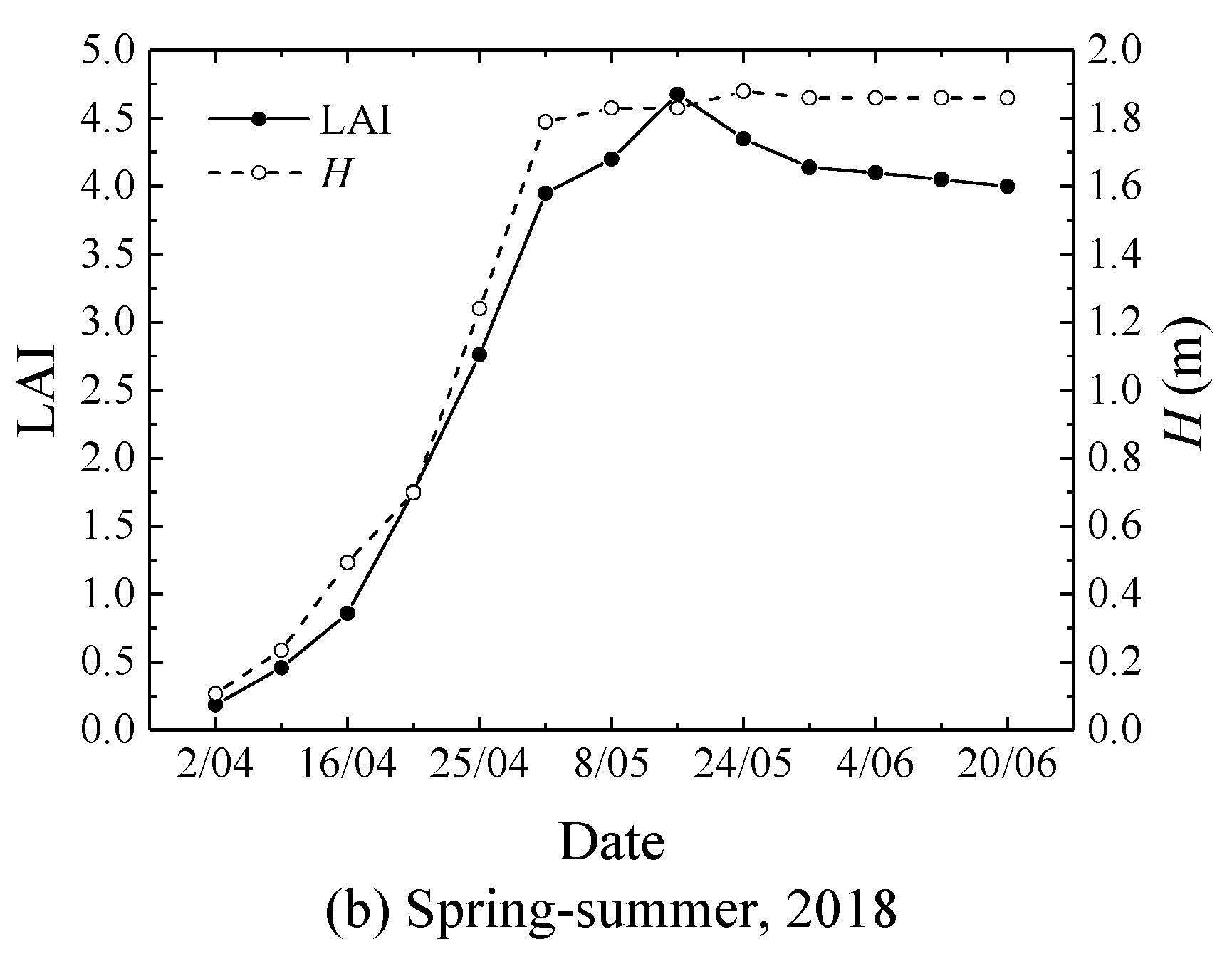
The experiment was performed in a 640 m² (32 m × 20 m) compartment of a Venlo-type glasshouse oriented east to west and located in Jiangsu University in Zhenjiang, China (latitude 32°11′ N, longitude 119°25 E; 23 m altitude). The experimental site was in a humid, subtropical, monsoon climatic zone with an average annual T_a of 15.5 °C and a mean annual precipitation (rainfall) of 1058.8 mm y⁻¹ [25]. The greenhouse consisted of three compartments, including a west and an east compartment each with two spans and middle compartment with one span, and was covered with a 4 mm float glass with transmittance greater than 89% [26]. Greenhouse forced ventilation was performed by two (1.5 m in diameter) axial fans fixed in the east wall of greenhouse [27]. More details of greenhouse construction were described by Yan et al. [27].

2.2. Crop

Cucumber seedlings (F1-HYBRID) were transplanted into the field on 3 September 2017 (autumn planting season) and 23 March 2018 (spring planting seasons) at a plant density equal to 6.63 per m² [26]. Seedlings were sowed 30 days before transplanting. The planting medium used in the greenhouse was a soil–biochar mixture with a mean bulk density of 1.266 g cm⁻³, a field capacity of 0.408 cm³ cm⁻³, and a permanent wilting-point water content of 0.16 cm³ cm⁻³ at a depth of 0–30 cm [25,26]. Three representative cucumber plants were transplanted into 3 lysimeters (30 cm in diameter and 50 cm in depth) and the soil was covered with clear polyethylene film to prevent evaporation [26]. The lysimeters were placed in the greenhouse with same density as plants in the troughs [25,26]. Irrigation was provided via an automatic drip irrigation system with dripping wings along the row and distributors 20 cm apart giving 100 mL min⁻¹. In order to keep the seedlings alive and to enhance growth, every plant was irrigated with 1 L on the transplanting date [26]. The crop was watered according to the accumulative pan (20 cm in diameter) evaporation (E_p) method. When the E_p reached 20 mm, the crop was irrigated to 18 mm (1.20 L) [26]. Liu et al. [28] demonstrated that 0.9E_p represented sufficient irrigation at 20 mm based on several years of experimental research in a solar greenhouse [26].

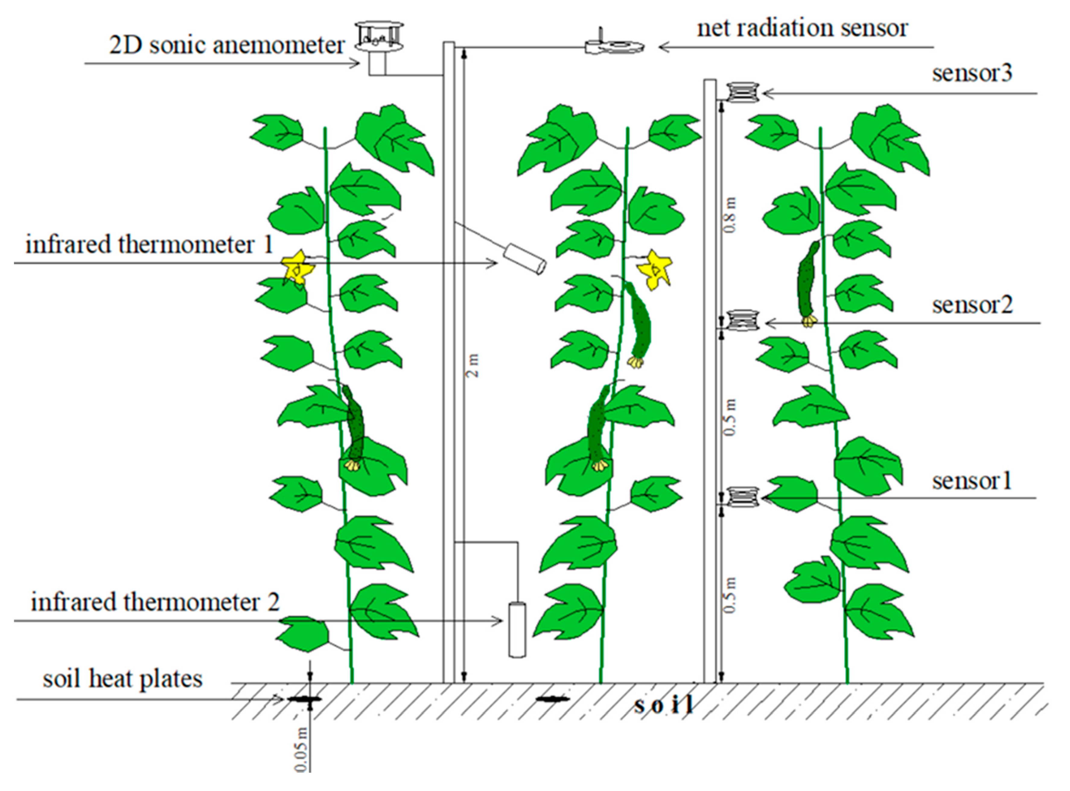
2.3. Instrumentation

The net radiation inside the greenhouse was measured with an NR (Net Radiometer) Lite 2 (Kipp and Zonen, Delft, the Netherlands) mounted at 2.5 m above the ground and centered over the crops. The sensitivity of the sensor was 10 μV/ (W m⁻²) with an accuracy of ±1%. Air velocity in the greenhouse was measured using a 2D sonic anemometer 1405-PK-021 (Gill, London, UK) at the same height. The soil heat flux was measured by two soil heat plates, HFP01-L10 (Campbell, CA, US), placed at 0.05 m below the soil surface. The leaf and soil surface temperatures were measured by two infrared thermometers, SI-111 (Campbell, CA, US), inside the canopy, as shown in Figure 1. The distance between the crop and thermometer 1 was about 0.5 m, and the horizontal angle between the leaves and thermometer 1 was about 45°; thermometer 2 was perpendicular to the soil surface. The data were collected and averaged every 10 min using a data logger system, CR1000 (Campbell, CA, US). The T_a and RH profiles were measured using three sensors (Onset Computer Corp, MA, US) at 0.5 m (sensor 1), 1.0 m (sensor 2), and 1.8 m (sensor 3) above the ground. A schematic view of the sensor locations is depicted in Figure 1. Solar radiation and air pressure were measured with an automatic weather station Hobo (Onset Computer Corp, MA, US) at 2.0 m above the ground. More details of the instrumentation were described by Yan et al. [25]. Nine of the newest fully developed mature leaves from sun-exposed terminal branches of three representative cucumber plants were selected to measure the leaf stomatal conductance (g_s), with the average data taken from three different leaves on the same plant [26]. The g_s was measured every half an hour using GFS (Gas-Exchange and Fluorescence System) -3000 (WALZ, Effeltrich, Germany) from 07:00 to 18:00 on sunny days, namely, 17 April, 23 May, and 22 June 2018 [26]. In this study, we used the measured g_s to parametrize r_c and integrate it into the SM model to validate the accuracy of the r_c submodel over two seasons.

The leaf area and the plant height of the cucumber plants were measured at intervals of 5–7 days. The leaf length (L) and the highest leaf width (W) were manually measured using a tape measure, and the conversion coefficient of 0.674 for the leaf area was derived from fitting the measured results to the one drawn using CAD (Computer Aided Design) software [25].

The T_r for three representative cucumber plants were measured by three balances (METTLER TOLEDO, Greifensee, Switzerland) with an accuracy of ±1 g, and the data were collected using a CR1000 data logger (Campbell, CA, US). The T_r of the crop ground area (W m⁻²) was calculated using the following formulae [15]:

$$T_r=\lambda \frac{{(m}_{t(i+1)}-m_{ti})}{{A\times (t}_{i+1}-t_i)},$$

(1)

$$A=\frac{a\times b}{n},$$

(2)

where λ is the latent heat of vaporization (J kg⁻¹), m_ti is the mass (kg) given by the balance at time t_i (s), n is the number of plants, a and b are the length (m) and the width (m) of the plot, and A (m²) is the actual area of one plant. Data from the balance were directly recorded every 10 min, 1 h, and 24 h. In this study, data on the 10 min scale were used for calculations and analysis.

2.4. Theoretical Model

2.4.1. Stanghellini Model (SM)

Stanghellini [8] stated that a canopy behaves, with respect to heat and vapor transfer, as a leaf of unit area with r_c and r_a, which are the corresponding resistances of one “real” leaf, divided by 2·LAI to get the equations:

$$T_r=\frac{\Delta \left(R_n-G\right)+\frac{{2\mathrm{LAI}\rho }_a{c}_p\mathit{VPD}}{r_a}}{{\Delta +\gamma }^{*}},$$

(3)

and

$${\gamma }^{*}=\gamma (1+\frac{r_c}{r_a}),$$

(4)

where R_n is the net radiation flux absorbed by the crop (W m⁻²), γ is the psychrometric constant (γ = 66 Pa °C⁻¹), c_p is the specific heat of air (J kg °C⁻¹), ρ_a is the density of air (kg m⁻³), VPD is the vapor pressure deficit of the air (Pa), and Δ is the slope of the saturated water vapor pressure curve (Pa °C⁻¹).

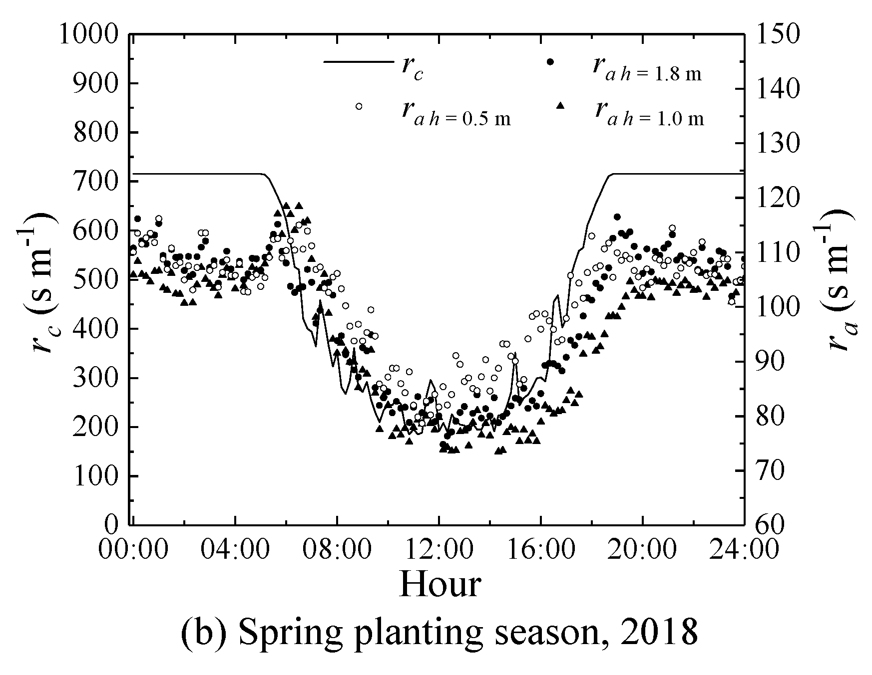
2.4.2. Aerodynamic Resistance and Canopy Resistance

The most physical method to evaluate r_a involves considering the leaf as a flat plate and deducing r_a from the determination of the heat exchange coefficient h_s induced by the airflow using dimensionless numbers [15]:

$$r_a=\frac{{\rho }_a{\times c}_p}{\mathrm{LAI}\times h_s},$$

(5)

where h_s (W m⁻²K⁻¹) is expressed as a function of the Nusselt number N_u.

According to the flat plate theory,

$$h_s=\frac{N_u\times d}{{\lambda }_a},$$

(6)

and the characteristic dimension of the leaf (m), d can be calculated as follows [29]:

$$d=\frac{2}{(1/L+1/W)}.$$

(7)

When Re² ≈ Gr and 10³ < Gr < 10⁹ in the greenhouse,

$$Nu=0{.68(\mathit{Re}}^{(3/2)}{+\mathit{Gr}}^{(3/4)}{)}^{1/3},$$

(8)

$$\mathit{Re}=\frac{{\rho }_a\mathit{Vd}}{{\mu }_a},$$

(9)

and

$$G_r=\frac{{g\times \beta \times \Delta T\times d}^3{\times \rho }_a^2}{{\mu }_a^2},$$

(10)

where L and W are the length (m) and the width (m) of the leaf, respectively, λ_a (W m⁻¹ K⁻¹) is the air thermal conductivity, R_e is Reynolds number, V (m s⁻¹) is the air speed, μ_a (Pa s) is the air dynamic viscosity, g (m s⁻²) is the acceleration of gravity, β (K ⁻¹) is the volumetric thermal expansion coefficient, and ΔT (K) is the temperature difference between the air and the leaf.

Canopy resistance (r_c) is usually estimated from the stomatal resistance (r_s) [20], considered to be the bulk stomatal resistance and representing the stomatal response of the “big leaf” [27]. The r_c is estimated from r_s as [30]

$$r_c=\frac{2r_s}{\mathrm{LAI}},$$

(11)

The inverse of the leaf stomatal conductance (g_s, mol m⁻² s⁻¹) is the stomatal resistance (r_s, s m⁻¹). The volume of 1 mol of gas is 0.0224 m³ at standard atmospheric pressure, i.e.,

$$r_s=\frac{1}{{0.0224\times g}_s},$$

(12)

2.4.3. Statistical Analysis

The coefficient of regression (a), the Root Mean Square Error (RMSE), the coefficient of determination (R²), and the modeling efficiency (EF) were calculated to validate the accuracy of the SM.

The a is given by

$$a=\frac{{{\displaystyle \sum }}_{i=1}^n{(O}_i{\times P}_i)}{{{\displaystyle \sum }}_{i=1}^n{O}_i{}^2},$$

(13)

which is the regression with predicted (P_i) and observed (O_i) values assuming the proportionality between the T_r calculated by the SM and the measurements taken by the lysimeters, where a is a proportionality constant.

The R² computed using the ordinary least squares is defined as

$$R^2=\frac{{\displaystyle {\sum }_{i=1}^n(O_i-\overline{O})(P_i-\overline{P})}}{\sqrt{{(O_i-\overline{O})}^2}\sqrt{{(P_i-\overline{P})}^2}},$$

(14)

where R² represents the proportion of the variance of the P_i as is explained by their regression on the observed values O_i.

The RMSE, computed as

$$\mathit{RMSE}=\sqrt{\frac{{{\displaystyle \sum }}_{i=1}^n{{(O}_i-P_i)}^2}{n}},$$

(15)

measures the overall difference between the predicted (P_i) and observed (O_i) values.

The EF is computed as

$$EF=1-\frac{{\displaystyle {\sum }_{i=1}^n{(O_i-P_i)}^2}}{{\displaystyle {\sum }_{i=1}^n{(O_i-\overline{O})}^2}},$$

(16)

where EF is the ratio between the Mean Square Error (MSE) of the predicted (P_i) values and the observed (O_i) values.

3. Results and Discussions

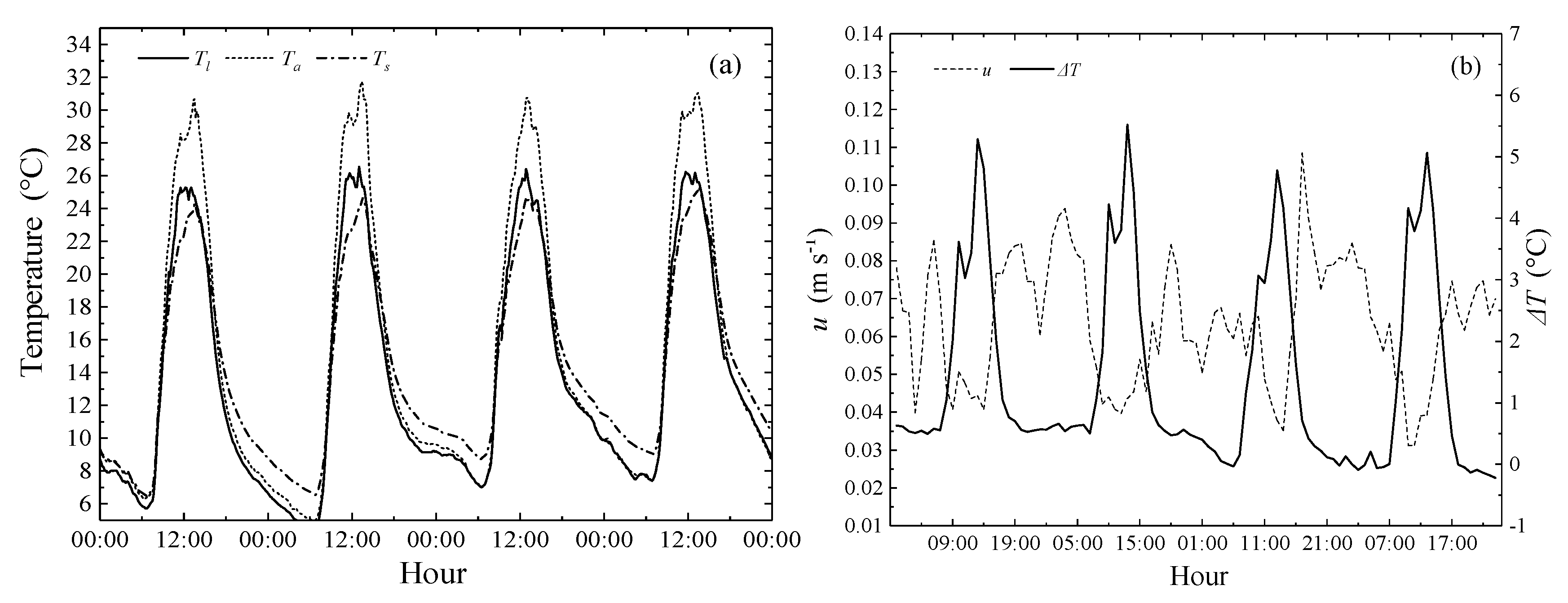
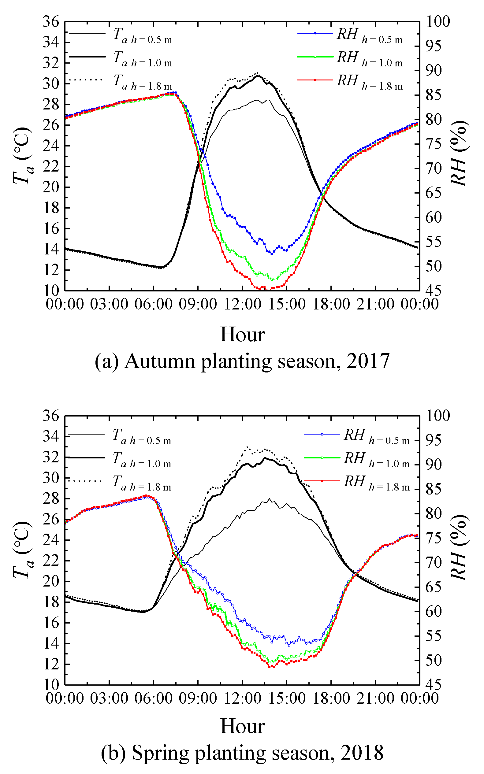
3.1. Meteorological Characterization in Greenhouse

The daily variations of meteorological data in the greenhouse in the middle stage of cucumber growth (23–26 November, 2017) are shown in Figure 2. The daily evolutions of leaf surface temperature T_l, soil surface temperature T_s, and air temperature T_a (above the crop) varied similarly; T_l varied from 4.28 to 26.55 °C with an average value of 13.42 °C, while T_a varied from 4.94 to 31.71 °C with an average value of 14.80 °C and T_s varied from 6.44 to 25.30 °C with an average value of 14.17 °C (Figure 2a). During night-time, T_s was higher than T_a because the soil stored the heat during the daytime, while T_s was several degrees (about 4.5 °C) lower than T_a at midday because the crop canopy intercepted some of the solar radiation. T_l was lower than T_a and the maximum difference between T_l and T_a was 6.3 °C. These results were in agreement with the findings of Yang et al. [19] and Papadakis et al. [31], who reported lower T_l values in greenhouse cucumber and tomato crops, respectively, compared to T_a during the whole day. Figure 2b shows the daily evolution of wind speed u (m s⁻¹) inside the greenhouse and the variation of the difference between T_a and T_l (ΔT, °C). The u was low and ranged from 0.03 to 0.11 (m s⁻¹). Regular increases in u occurred during night-time when the ΔT was low, indicating that T_l approached T_a at higher u in the greenhouses. Stanghellini [8] reported similar results and suggested that a fan could be used as a reasonable cooling device to lower the ΔT, thereby reducing the T_r in greenhouses.

Figure 3 shows the T_a and RH at three heights (0.5, 1.0, and 1.8 m) above the ground near the cucumber plants during (a) the autumn planting season and (b) the spring planting season. During the daytime, the highest value of T_a was observed 1.8 m above the ground, with the T_a decreasing significantly with the observation height. The maximum decrease in T_a at heights of 1.8 m to 1.0 m and 0.5 m above the ground were 4.84% and 11.01% during the autumn planting season, while for the spring planting season, the maximum decreases in T_a from the height of 1.8 m to 1.0 m and 0.5 m above the ground were 4.76% and 18.61%. However, no significant differences in T_a among the three observation heights were observed during night-time. For RH, during the daytime, the highest value of RH was observed at the lowest observation height (0.5 m), where the T_a was the lowest. The maximum differences in RH at 0.5 m and 1.8 m reached 10.49% and 6.24% for the two planting seasons, respectively. The greenhouse cucumber crop was thus characterized by a strong vertical micrometeorological gradient, with high T_a and low RH at the top of the crop canopy (1.8 m above ground) and much more moderate micrometeorological condition at its base (0.5 m above the ground). This result was in agreement with the observations made by Demrati et al. [14], who studied banana trees in a naturally ventilated greenhouse.

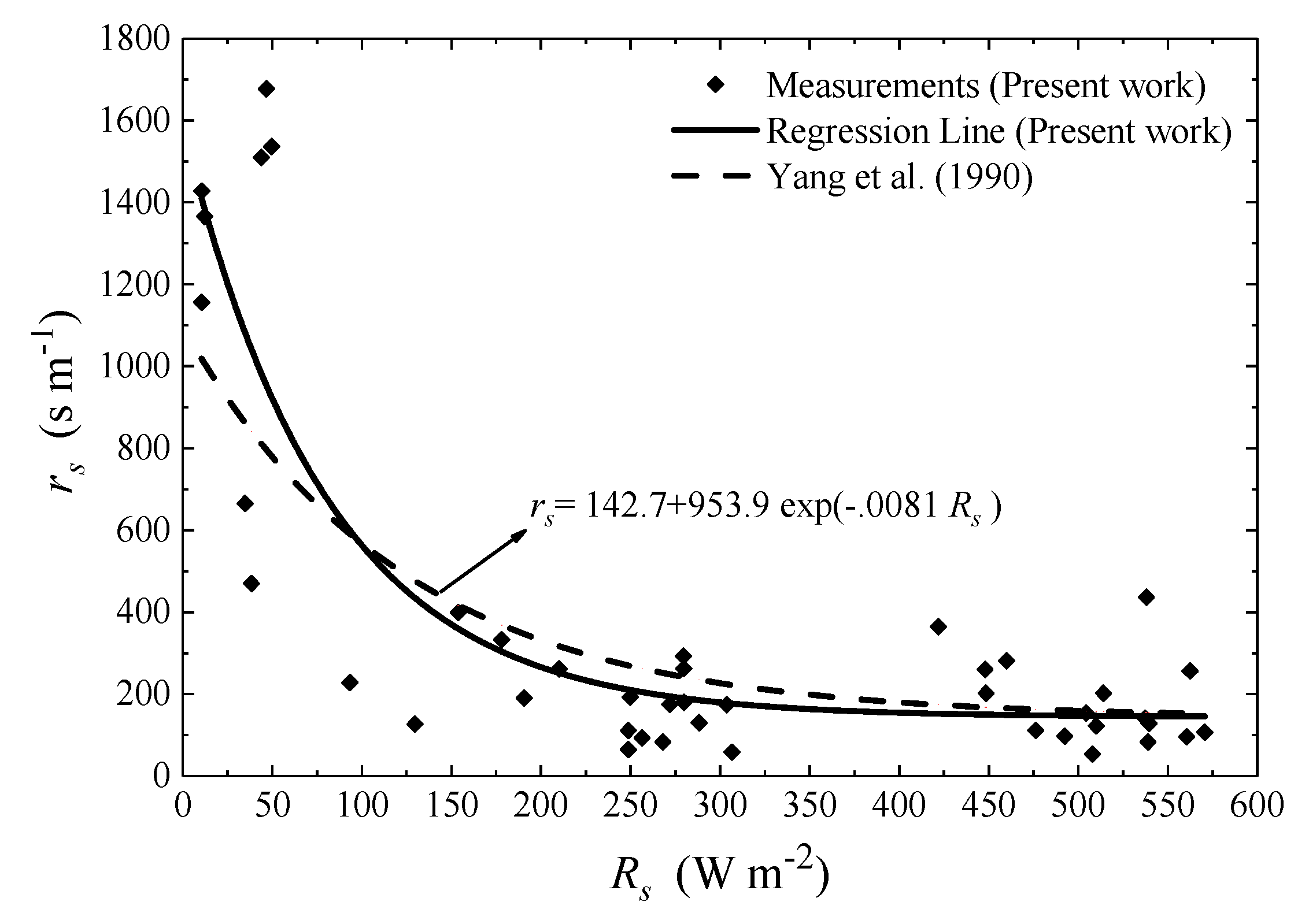
3.2. Parametrization of the Stanghellini Model (SM)

The variations in LAI and plant height (H) are shown in Figure 4. The LAI reached a maximum of 4.08 in early November and the H reached a maximum of 1.88 m in mid-November during the autumn planting season. The LAI reached a maximum of 4.67 in mid-May and the H reached a maximum of 1.86 m during the spring planting season. In this study, the growing periods (2–10 November 2017 and 2–10 May 2018) of the LAI and H were 4 and 1.8 m, respectively.

Canopy resistance (r_c) is usually estimated from the stomatal resistance (r_s), which is often estimated through a set of environmental variables [5,20]. Yang et al. [19] proved that no significant correlations between the r_s and other climatic variables were found, except for the solar radiation (R_s) of cucumber plants in greenhouses. A best-fit exponential equation for the R_s and r_s of the cucumber plants was obtained, as follows:

$$r_s=144.3+1440.4\exp (-0.0124\times R_s),$$

(17)

where R² = 0.74 and RMSE = 160.4 s m⁻¹. Similar results regarding the effects of R_s on the r_s of the cucumber crop were observed in cucumber by Yang et al. [19], but with some differences in the model coefficients (Figure 5). The difference in the cucumber cultivars and geographical and meteorological conditions may have affected the model coefficients.

As shown in Figure 6, the r_c was higher during the morning and night but lower during the day. This behavior was mainly attributed to the stomata staying closed at night, thereby resulting in higher resistances to water transfer and stomata opening for photosynthesis during daytime, which also drastically reduced the resistances [9,32]. The average values of r_c during the day were 345 and 292 s m⁻¹, but 750 s m⁻¹ during the morning and night for the autumn and spring planting seasons, respectively. These results were in agreement with the values that Yang et al. [19] obtained for cucumber plants grown in an intelligent greenhouse.

According to the relative magnitude of R_e and G_r, when G_r/R_e² ≥ 10, pure free convection occurs, whereas when 0.1 < G_r/R_e² < 10, mixed convection occurs [33]. The results indicated that the air flow convection regime inside the greenhouse was mainly mixed convection (88.91%) and pure free convection occurred at midday (6.24%). Therefore, it was assumed that the air flow convection regime was mixed convection in the greenhouse in order to calculate the r_a. A similar result was reported by Qiu et al. [20] for a solar greenhouse in Northwest China. The r_{a h = 0.5 m}, r_{a h = 1.0 m}, and r_{a h = 1.8 m} denoted the average variations of the r_a values that were estimated based on the air temperature measured at three different heights (h = 0.5, 1.0, and 1.8 m) for nine consecutive days during two planting seasons, as shown in Figure 6. Values of r_{a h = 0.5 m}, r_{a h = 1.0 m}, and r_{a h = 1.8 m} were almost the same, except for slight differences (less than 10 s m⁻¹) between them at 08:00–16:00. The reason for this pattern was attributed to the three heights of T_a showing significant differences at 08:00–16:00, as shown in Figure 3. The value of r_a hovered around 100 s m⁻¹ and the average values of r_a were 108 and 98 s m⁻¹ during the two planting seasons. These values were relatively close to the results obtained by Zhang and Lemeur [34] (r_a = 133 s m⁻¹), who calculated the Nusselt number (N_u) according to the equation of Stanghellini [8] under similar greenhouse conditions, but were higher than the results given by Yan et al. [25] (r_a = 35 s m⁻¹), who used the inverse bulk transfer equation based on actual measurements of latent heat flux in the same greenhouse. Furthermore, Yan et al. [25] presented that sensible heat flux was sensitive to r_a errors, but with much less effect on the latent heat flux.

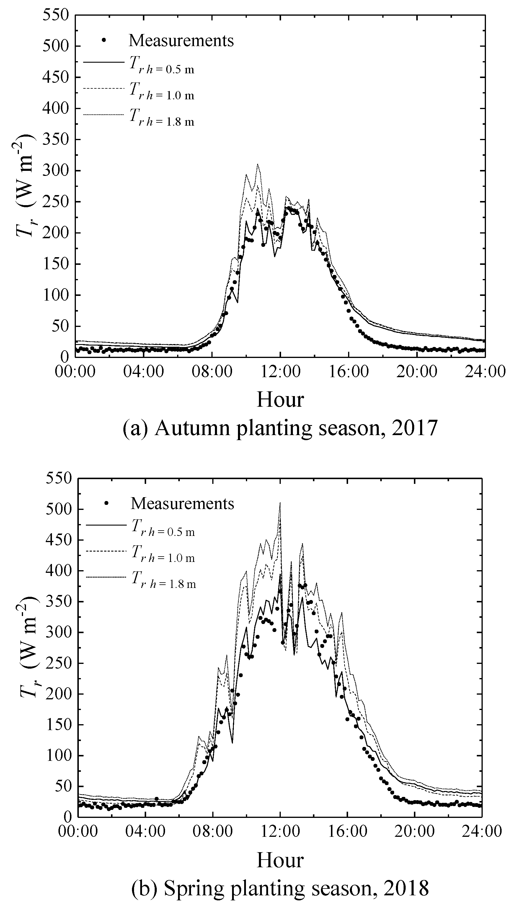
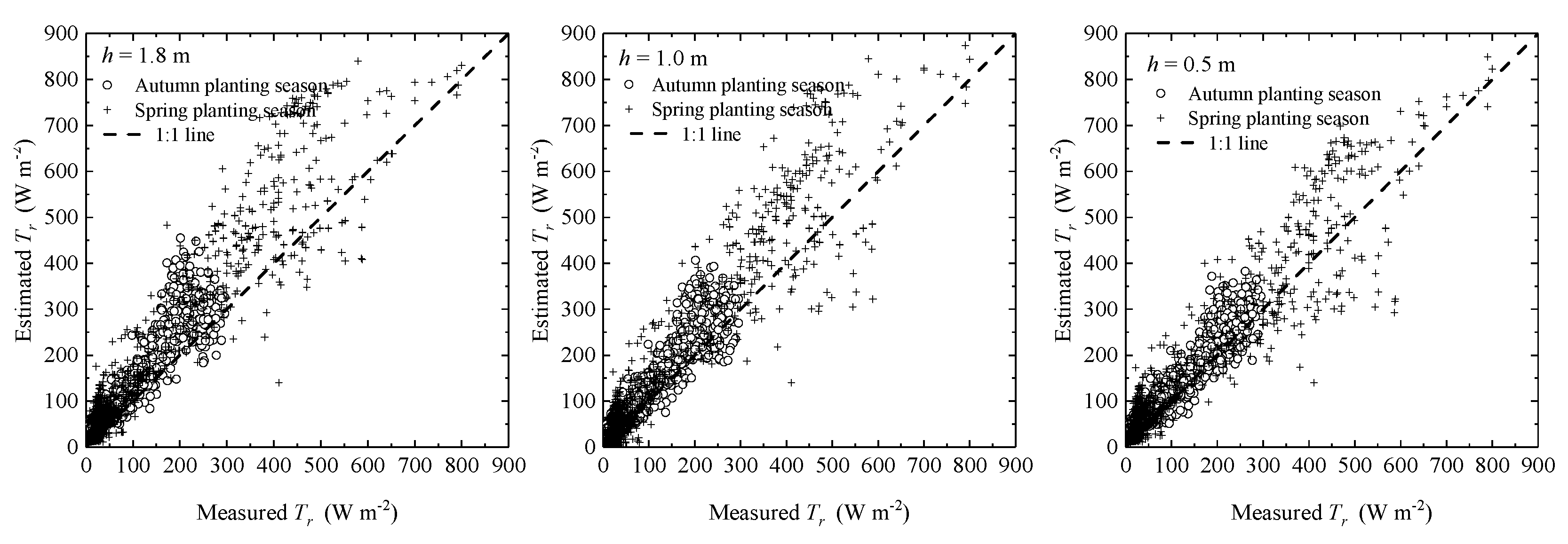
3.3. Effects of Micrometeorological Data Observation Heights on the Performance of the SM

The average variations of the measured and estimated T_r values for nine consecutive days (2–10 November 2017 and 2–10 May 2018) in the middle growing stages of the cucumber plants are shown in Figure 7. The T_{r h = 0.5 m}, T_{r h = 1.0 m}, and T_{r h = 1.8 m} represent the T_r estimated by the SM using the micrometeorological data observed at heights of 0.5, 1.0, and 1.8 m above the ground, respectively. The variations in the T_r values were not smooth during the daytime due to the variations in greenhouse energy caused by the R_s inside the greenhouse sometimes being intercepted by beams. Figure 7 illustrates that the T_r values estimated by the SM were close to the values that were measured by the lysimeters. At night, T_{r h = 1.8 m}, T_{r h = 1.0 m}, and T_{r h = 0.5 m} showed no significant differences and the SM overestimated the actual T_r, particularly after 16:00 pm; however, significant differences were observed as soon as the sun rose. The T_{r h = 1.8 m} and T_{r h = 1.0 m} overestimated the actual T_r by 17.14% and 7.69%, while T_{r h = 0.5 m} underestimated the actual T_r by 2.65% for the autumn planting season. Similar patterns were observed in the spring planting season, with the T_{r h = 1.8 m} and T_{r h = 1.0 m} overestimating the actual T_r by 27.65% and 17.58% and the T_{r h = 0.5 m} underestimating the actual T_r by 2.02% for the spring planting season. Morille et al. [15] reported the same phenomenon that the PM model produced, which highly overestimated the T_r by a maximum of 62.7% when using the micrometeorological data just above the crop for New Guinea Impatiens crop in a Venlo-type greenhouse.

Figure 8 shows comparisons of the T_r values estimated by the SM based on the micrometeorological data from three observation heights (h = 0.5, 1.0, and 1.8 m) and the values measured by the lysimeters. The T_r estimated by the SM based on the micrometeorological data measured at 0.5 m above the ground had the strongest correlation with the measured values, while the estimated T_r based on the data from 1.8 m had the weakest correlation with the measured values. The slope of regression lines of the measured and estimated T_r values based on the data from three heights (h = 0.5, 1.0, and 1.8 m) were 0.96, 1.21, and 1.3 for the autumn planting season and 0.98, 1.19, and 1.27 for the spring planting season, respectively. The EF and RMSE of the T_r estimated by the SM based on the data from the height of 0.5 m were 95% and 18 W m⁻², while the corresponding values were 86% and 29 W m⁻² in the case of 1.8 m above the ground for the autumn planting season. For the spring planting season, the EF and RMSE were 92% and 34 W m⁻² with the data observed at 0.5 m, while the corresponding values were 81% and 56 W m⁻² at 1.8 m. These results showed that the differences in the observation positions of the micrometeorological data used in the SM caused T_r overestimation. Therefore, applying the micrometeorological data measured at 0.5 m above the ground instead of measuring above the canopy in accordance with the SM caused better estimation of the T_r.

To further explain why the meteorological data inside the canopy was most accurate when used with the SM, Morille et al. [15] reported that due to the existence of hypostomatic plant stomata on the underside of leaves and sensible temperature and humidity gradients inside the canopy, it is logical to estimate the water vapor heat exchanges by considering the within-canopy air characteristics. Yang [23] claimed that the evaluation of resistance parameters based on dimensionless numbers uses the micrometeorological data measured above the crop, meaning that both the water vapor transferred resistances between the crop and the inside-canopy air and between the inside of the canopy and above it are taken into account, which is undesirable; therefore, it reasonable to use the inside-crop micrometeorological data to evaluate the resistance parameters. In our study, we found that T_{r h = 1.0 m} overestimated the actual T_r and T_{r h = 0.5 m} underestimated the actual T_r; therefore, we recommend that T_r estimations of cucumber should use inside-canopy micrometeorological data.

The overall values RMSE, R², and EF values in this study, which were 26.19 W m⁻², 0.92, and 93.19%, respectively, (

Table 1. Statistical analysis of the measured and estimated T_r values using the SM in accordance with data from 2 to 10 November 2017 and from 2 to 10 May 2018.

Measured Heights	${\overline{T}}_r$estimated	${\overline{T}}_r$measured	a	R2	RMSE	EF
h = 1.8 m	123.08	91.40	1.29	0.92	42.86	83.29%
h = 1.0 m	112.85	91.40	1.20	0.94	31.71	90.01%
h = 0.5 m	108.11	91.40	0.97	0.91	26.19	93.19%

Note: ${\overline{T}}_r$ _estimated and ${\overline{T}}_r$ _measured were the averaged values of T_r estimated by the SM and measured using a lysimeter (W m⁻²), respectively; a is the slope of the least square regression line, R² is the coefficient of determination, RMSE is the Root Mean Square Error (W m⁻²), and EF is modeling efficiency.

), showed that the SM was appropriately applied to the precise irrigation scheduling of greenhouse cucumber crops. Water balance [35,36], remote sensing methods, [2,36] and thermal infrared remote techniques [2,37] have been developed to measure plant water use, however, for crop irrigation scheduling applications, the results of the above methods still require verification using field data before practical application. In this study, the SM’s mathematical relations and physical models were precise, viable, and accepted tools for the development of location-specific water use for irrigation scheduling.

4. Conclusions

This study emerged from the need to develop accurate models to estimate the transpiration (T_r) of cucumber plants within greenhouses. An experiment was conducted in a Venlo-type greenhouse in South China. Micrometeorological data observed at three different heights were applied in the Stanghellini model (SM) to calculate the T_r compared to the measured values. The microclimate conditions in the Venlo-type greenhouse in South China were characterized by a strong vertical microclimatic gradient; the maximum decrease in RH from 0.5 m to 1.0 m above the ground was 11.05%, with 7.88% being the maximum decrease from 1.0 m to 1.8 m. The maximum difference in air temperature (T_a) at 0.5 m and 1.8 m reached 4.14 °C.

The canopy resistance (r_c) and aerodynamic resistance (r_a) in the SM were parametrized based on the stomatal resistance (r_s) and heat exchange coefficient (h_s), respectively. An empirical model of r_s was developed in accordance the solar radiation (R_s) inside the greenhouse, while r_a was determined using h_s based on dimensionless numbers. By integrating the parameterized r_c and r_a into the SM, the efficiency (EF) and Root Mean Square Error (RMSE) of the SM-estimated T_r values based on the micrometeorological data at a height of 0.5 m were 95% and 18 W m⁻², while the corresponding values were 86% and 29 W m⁻² at a height of 1.8 m for the autumn planting season. During the spring planting season, the EF and RMSE were 92% and 34 W m⁻² at 0.5 m above the ground, and the corresponding values were 81% and 56 W m⁻² at 1.8 m. The performance of the SM based on the micrometeorological data measured at three heights showed that application of the micrometeorological data at 0.5 m produced T_r estimates at the highest level of accuracy.

References

1. Luo, Y.F.; Traore, S.; Lyu, X.; Wang, W.G.; Wang, Y.; Xie, Y.Y.; Jiao, X.; Fipps, G. Medium Range Daily Reference Evapotranspiration Forecasting by Using ANN and Public Weather Forecasts. Water Resour. Manag. 2015, 29, 3863–3876. [Google Scholar] [CrossRef]
2. Han, W.T.; Sun, Y.; Xu, T.F.; Chen, X.W.; Su, K.O. Detecting maize leaf water status by using digital rgb images. Int. J. Agric. Biol. Eng. 2014, 7, 45–53. [Google Scholar]
3. Xu, D.; Li, Y.N.; Gong, S.H.; Zhang, B.Z. Waterlogging and saline-alkaline management for development of sustainably irrigated agriculture. J. Drain. Irrig. Mach. Eng. 2019, 37, 63–72, (In Chinese with English abstract). [Google Scholar]
4. De, J.S.; Guo, P.; Zhang, C.L.; Yue, Q.; Shan, B.Y. Optimal allocation of irrigation water resources based on meteorological factor under uncertainty. J. Drain. Irrig. Mach. Eng. 2019, 37, 540–544, (In Chinese with English abstract). [Google Scholar]
5. Allen, R.G.; Pereira, L.S.; Raes, D.; Smith, M. Crop Evapotranspiration—Guidelines for Computing Crop Water Requirements; FAO Irrigation and Drainage Paper 56; FAO: Rome, Italy, 1998; p. 300. [Google Scholar]
6. Penman, H.L. Natural evaporation from open water, bare soil and grass. Proc. R. Soc. London A Math. Phys. Eng. Sci. 1948, 1032, 120–145. [Google Scholar]
7. Monteith, J.L. Evaporation and environment. In Symposia of the Society for Experimental Biology; University Press: Cambridge, UK, 1965; pp. 206–234. [Google Scholar]
8. Stanghellini, C. Transpiration of Greenhouse Crops: An Aid to Climate Management. Ph.D. Thesis, Agricultural University of Wageningen, Wageningen, The Netherlands, 1987; 150p. [Google Scholar]
9. Villarreal-Guerrero, F.; Kacira, M.; Fitz-Rodríguez, E.; Kubota, C.; Giacomelli, G.A.; Linker, R.; Arbel, A. Comparison of three evapotranspiration models for a greenhouse cooling strategy with natural ventilation and variable high pressure fogging. Sci. Hortic. 2012, 134, 210–221. [Google Scholar] [CrossRef]
10. Jolliet, O.; Bailey, B.J. The effect of climate on tomato transpiration in greenhouses: Measurements and models comparison. Agric. For. Meteorol. 1992, 58, 43–62. [Google Scholar] [CrossRef]
11. Prenger, J.J.; Fynn, R.P.; Hansen, R.C. A comparison of four evapotranspiration models in a greenhouse environment. Trans. ASAE 2002, 45, 1779–1788. [Google Scholar] [CrossRef]
12. Lopez-Cruz, I.L.; Olivera-Lopez, M.; Herrera-Ruiz, G. Simulation of greenhouse tomato crop transpiration by two theoretical models. Acta Hortic. 2008, 797, 145–150. [Google Scholar] [CrossRef]
13. Pamungkas, A.P.; Hatou, K.; Morimoto, T. Evapotranspiration model analysis of crop water use in plant factory system. Environ. Control Biol. 2014, 52, 183–188. [Google Scholar] [CrossRef] [Green Version]
14. Demrati, H.; Boulard, T.; Fatnassi, H.; Bekkaoui, A.; Majdoubi, H.; Elattir, H.; Bouirden, L. Microclimate and transpiration of a greenhouse banana crop. Biosyst. Eng. 2007, 98, 66–78. [Google Scholar] [CrossRef]
15. Morille, B.; Migeon, C.; Bournet, P.E. Is the Penman-Monteith model adapted to predict crop transpiration under greenhouse conditions? Application to a New Guinea Impatiens crop. Sci. Hortic. 2013, 152, 80–91. [Google Scholar] [CrossRef]
16. Yan, H.F.; Zhang, C.; Oue, H.; Peng, G.J.; Darko, R.O. Determination of crop and soil evaporation coefficients for estimating evapotranspiration in a paddy field. Int. J. Agric. Biol. Eng. 2017, 10, 130–139. [Google Scholar]
17. Katerji, N.; Rana, G.; Fahed, S. Parameterizing canopy resistance using mechanistic and semi-empirical estimates of hourly evapotranspiration: Critical evaluation for irrigated crops in the Mediterranean. Hydrol. Process. 2011, 25, 117–129. [Google Scholar] [CrossRef]
18. Yan, H.F.; Zhang, C.; Peng, G.J.; Darko, R.; Cai, B. Modelling canopy resistance for estimating latent heat flux at a tea field in south China. Exp. Agric. 2018, 54, 563–576. [Google Scholar] [CrossRef]
19. Yang, X.S.; Short, T.H.; Fox, R.D.; Bauerle, W.L. Transpiration, leaf temperature and stomatal resistance of greenhouse cucumber crop. Agric. For. Meteorol. 1990, 51, 197–209. [Google Scholar] [CrossRef]
20. Qiu, R.J.; Kang, S.Z.; Du, T.S.; Tong, L.; Hao, X.M.; Chen, R.Q.; Chen, J.L.; Li, F.S. Effect of convection on the Penman-Monteith model estimates of transpiration of hot pepper grown in solar greenhouse. Sci. Hortic. 2013, 160, 163–171. [Google Scholar] [CrossRef]
21. Gong, X.W.; Liu, H.; Sun, J.S.; Gao, Y.; Zhang, X.X.; Shiva, K.J.H.A.; Zhang, H.; Ma, X.J.; Wang, W.N. A proposed surface resistance model for the Penman-Monteith formula to estimate evapotranspiration in a solar greenhouse. J. Arid Land 2017, 9, 530–546. [Google Scholar] [CrossRef]
22. Jarvis, P.G. The interpretation of the variations in leaf water potential and stomatal conductance found in canopies in the field. Philos. Trans. R. Soc. B Biol. Sci. 1976, 273, 593–610. [Google Scholar]
23. Yang, X.S. Greenhouse micrometeorology and estimation of heat and water vapor fluxes. J. Agric. Eng. Res. 1995, 61, 227–237. [Google Scholar] [CrossRef]
24. Kittas, C.; Katsoulas, N.; Baille, A. Influence of misting on the diurnal hysteresis of canopy transpiration rate and conductance in a rose greenhouse. Acta Hortic. 2000, 534, 155–161. [Google Scholar] [CrossRef]
25. Yan, H.F.; Zhang, C.; Gerrits, M.C.; Acquah, S.J.; Zhang, H.N.; Wu, H.M.; Zhao, B.S.; Huang, S.; Fu, H.W. Parametrization of aerodynamic and canopy resistances for modeling evapotranspiration of greenhouse cucumber. Agric. For. Meteorol. 2018, 262, 370–378. [Google Scholar] [CrossRef]
26. Huang, S.; Yan, H.F.; Zhang, C.; Wang, G.Q.; Acquah, S.J.; Yu, J.J.; Li, L.L.; Ma, J.M.; Opoku Darko, R. Modeling evapotranspiration for cucumber plants based on the Shuttleworth-Wallace model in a Venlo-type greenhouse. Agric. Water Manag. 2020, 228, 105861. [Google Scholar] [CrossRef]
27. Yan, H.F.; Acquah, S.J.; Zhang, C.; Wang, G.Q.; Huang, S.; Zhang, H.N.; Zhao, B.S.; Wu, H.M. Energy partitioning of greenhouse cucumber based on the application of Penman-Monteith and Bulk Transfer models. Agric. Water Manag. 2019, 217, 201–211. [Google Scholar] [CrossRef]
28. Liu, H. Water Requirement and Optimal Irrigation Index for Effective Water Use and High-Quality of Tomato in Greenhouse. Ph.D. Thesis, Chinese Academy of Agricultural Sciences, Beijing, China, 2010. (In Chinese with English abstract). [Google Scholar]
29. Montero, J.I.; Anton, A.; Munoz, P.; Lorenzo, P. Transpiration from geranium grown under high temperatures and low humidities in greenhouses. Agric. For. Meteorol. 2001, 107, 323–332. [Google Scholar] [CrossRef]
30. Pirkner, M.; Dicken, U.; Tanny, J. Penman-Monteith approaches for estimating crop evapotranspiration in screenhouses—A case study with table-grape. Int. J. Biometeorol. 2014, 58, 725–737. [Google Scholar] [CrossRef]
31. Papadakis, G.; Frangoudakis, A.; Kyritsis, S. Experimental investigation and modelling of heat and mass transfer between a tomato crop and the greenhouse environment. J. Agric. Eng. Res. 1994, 57, 217–227. [Google Scholar] [CrossRef]
32. Acquah, S.J.; Yan, H.F.; Zhang, C.; Wang, G.Q.; Zhao, B.S.; Wu, H.M.; Zhang, H.N. Application and evaluation of Stanghellini model in the determination of crop evapotranspiration in a naturally ventilated greenhouse. Int. J. Agric. Biol. Eng. 2018, 11, 95–103. [Google Scholar]
33. Wang, H.H.; Zhou, G.M.; Li, X.Y. Heat Transfer Theory; Chongqing University Press: Chongqing, China, 2006; 185p. [Google Scholar]
34. Zhang, L.; Lemeur, R. Effect of aerodynamic resistance on energy balance and Penman—Monteith estimates of evapotranspiration in solar greenhouse conditions. Agric. For. Meteorol. 1992, 58, 209–228. [Google Scholar] [CrossRef]
35. Allen, R.G.; Pereira, L.S.; Howell, T.A.; Jensen, M.E. Evapotranspiration information reporting: I. Factors governing measurement accuracy. Agric. Water Manag. 2011, 98, 899–920. [Google Scholar] [CrossRef] [Green Version]
36. Choudhury, B.U.; Singh, A.K.; Pradhan, S. Estimation of crop coefficients of dry-seeded irrigated rice—Wheat rotation on raised beds by field water balance method in the indo-gangetic plains, India. Agric. Water Manag. 2013, 123, 20–31. [Google Scholar] [CrossRef]
37. Tian, F.; Hou, M.; Qiu, Y.; Zhang, T.; Yuan, Y. Salinity stress effects on transpiration and plant growth under different salinity soil levels based on thermal infrared remote (TIR) technique. Geoderma 2020, 357, 113961. [Google Scholar] [CrossRef]
Figure 1. A schematic view of the sensor locations.
Water 12 00517 g001
Figure 2. Time course of leaf surface temperature Tl, soil surface temperature Ts and air temperature Ta (a); wind speed u, and the temperature difference between Ta and TlT) (b) from 23 to 26 November 2017.
Water 12 00517 g002
Figure 3. Time evolution of average air temperature (Ta) and relative humidity (RH) at three observation heights (0.5, 1.0, and 1.8 m above the ground) (a) from 2 to 10 November 2017 (autumn planting season) and (b) from 2 to 10 May 2018 (spring planting season).
Water 12 00517 g003
Figure 4. Evolution of plant height (H) and leaf area index (LAI) during cucumber growth in 2017 (a) and 2018 (b). The transplanting and harvesting dates were 3 September and 12 December in 2017, respectively, and 23 March and 29 June in 2018, respectively.
Water 12 00517 g004aWater 12 00517 g004b
Figure 5. Correlations of the stomatal resistance (rs) with solar radiation (Rs) from 07:00 to 18:00 on 17 April, 23 May, and 22 June 2018.
Water 12 00517 g005
Figure 6. Average variations of rc and ra (s m−1) in (a) the autumn planting season (from 2 to 10 November 2017) and (b) the spring planting season (from 2 to 10 May 2018).
Water 12 00517 g006aWater 12 00517 g006b
Figure 7. Variations of the measured and estimated average Tr values by the Stanghellini model (SM) based on the meteorological data at three observation heights (a) from 2 to 10 November 2017 and (b) from 2 to 10 May 2018.
Water 12 00517 g007
Figure 8. Comparisons of the Tr estimated by the SM based on meteorological data at three observation heights and data measured using a lysimeter during the autumn (2 to 10 November 2017) and spring (2 to 10 May 2018) planting seasons.
Water 12 00517 g008