A Deterministic Monte Carlo Simulation Framework for Dam Safety Flow Control Assessment


Department of Civil and Environmental Engineering, Western University, London, ON N6A3K7, Canada
*
Author to whom correspondence should be addressed.
Water 2020, 12(2), 505; https://doi.org/10.3390/w12020505
Submission received: 17 December 2019
/
Revised: 5 February 2020
/
Accepted: 5 February 2020
/
Published: 12 February 2020
(This article belongs to the Special Issue Planning and Management of Hydraulic Infrastructure)
Abstract
:Simulation has become more widely applied for analysis of dam safety flow control in recent years. Stochastic simulation has proven to be a useful tool that allows for easy estimation of the overall probability of dam overtopping failure. However, it is difficult to analyze “uncommon combinations of events” with a stochastic approach given current computing abilities, because (a) the likelihood of these combinations of events is small, and (b) there may not be enough simulated instances of these rare scenarios to determine their criticality. In this research, a Deterministic Monte Carlo approach is presented, which uses an exhaustive list of possible combinations of events (scenarios) as a deterministic input. System dynamics simulation is used to model the dam system interactions so that low-level events within the system can be propagated through the model to determine high-level system outcomes. Monte Carlo iterations are performed for each input scenario. A case study is presented with results from a single example scenario to demonstrate how the simulation framework can be used to estimate the criticality parameters for each combination of events simulated. The approach can analyze these rare events in a thorough and systematic way, providing a better coverage of the possibility space as well as valuable insights into system vulnerabilities.
1. Introduction
Typical dam safety assessments tend to focus on analyzing a subjectively chosen group of scenarios, often at or near the edge of the design envelope, analyzed probabilistically using event tree analysis. Event trees are a useful tool in quantification of probability, but are unable to model non-linear behavior, component interactions, and system feedbacks, which are often observed in dam failure. Event trees are unable to determine the dynamic system response to input conditions, which includes the resulting reservoir levels associated with a particular scenario. Regan [1] cites examples of dam failures, including Teton and Taum Sauk, in which non-linear behavior was observed, noting that event trees are too simplistic to anticipate the complex interactions occurring within various levels of a dam system.
In more recent years, a small group of researchers, beginning with Regan [1], began to point to systems approach as a potential path forward to overcome some issues associated with traditional approaches [2,3,4]. Baecher et al. [5] present the framework for a methodology for achieving such an approach using stochastic simulation, with events occurring randomly in a continuous simulation based on fragility curves.
Stochastic simulation (sometimes referred to as Monte Carlo simulation) is becoming more commonly applied within the dams industry for safety analysis [3,4,6]. Hartford et al. [3] describes several applications of this approach. In stochastic simulation, random failures of components may be initiated (with random outage lengths) to determine the overall probability of failure for the system. In this way, each run of a stochastic simulation model would produce a different output. If run for enough years, the probability of failure would begin to converge on a single value. Stochastic simulation is able to analyze component interactions, nonlinear behaviour, and overall likelihood of failure, making it the current state-of-the-art in dam safety risk assessment. Stochastic simulation models with an adequate amount of detail can capture feedback relationships between system components as well as dynamic and non-linear system behaviour, which is difficult to assess using traditional event tree analysis or the more recently proposed Bayesian network approach [7]. Stochastic simulation outputs for a dam system can include the reservoir level fluctuations and outflows in response to various inflows and constraints, which makes simulation a particularly promising tool for dam safety analysis. Stochastic simulation has the benefit of simplicity and easy estimation of the overall probability of flow control failure of a system. Analyzing the conditional probabilities of failure (and other parameters) for specific scenarios is not a direct output of a fully stochastic analysis, though it may be possible using data mining and a significantly large number of simulation years.
Hartford et al. [3] describe the “uncommon combination of common events” occurring well within the design envelope that could lead to dam failures. The ability to systematically analyze the full set of these potential combinations using stochastic simulation is inherently limited by the probabilities assigned to the events and the number of years run (computational limitations). Only a subset of the possible “combinations of events” will be analyzed using a typical stochastic simulation framework, and this subset will differ between two subsequent runs of the same model. Multiple events occurring and impacting one another are rare within a stochastic simulation (because they have a low combined probability of occurrence), but these scenarios are still important possibilities that contribute to the overall likelihood of flow-control failure for the system. These rare scenarios may only appear a few times, if at all, so a more thorough analysis of the scenarios themselves is limited. Each scenario will have a wide range of possible outcomes depending on the initial reservoir levels, inflows, and timing of events. The major limitation of the stochastic approach is that it is computationally prohibitive to conduct a thorough analysis of the combinations of events, and as such the approach may be unable to estimate the criticality of these unlikely, yet potentially dangerous, scenarios.
There is some recent work that could potentially be of value in improving the ability to assess these uncommon combinations of events. Recently, King et al. [8] developed an approach that automatically generates dam system operating scenarios from a component operating states database, using combinatorics. The database contains a complete list of the system components as well as their operating states (normal, failures, delays, errors, etc.) and causal factors. The combinatorial procedure then uses the database entries to generate a complete list of all possible combinations of operating states (scenarios). Each scenario contains a single operating state for each component in the dam system being considered. King et al. [8] also suggest event timing, inflows, and outage lengths for each scenario can be explored through Monte Carlo simulation. King et al. [9] present a system dynamics simulation model that represents, in detail, the components of a dam system and their interactions. The simulation model mathematically characterizes the system behavior using feedbacks and interactions within a hierarchical system of systems. The approach can analyze high-level system behavior using low-level failures and events as inputs. However, the model described by King et al. [9] is completely deterministic and does not provide a complete simulation framework capable of analyzing each of the potential combinations of events in an automated and systematic way. Another potential problem that has not yet been investigated is how to determine the start and end of a scenario, which depends on whether the preceding events in a scenario are influencing the events that follow.
In this paper, a Deterministic Monte Carlo framework is developed that can be utilized to systematically assess each of the combinations of events that can impact dam system flow-control. The process for determining these combinations of events is described by King et al. [8]. A brief description of the approach for developing and testing a system dynamics simulation model for a dam system is presented. The process for determining Monte Carlo simulation inputs and connecting them to the simulation model is also described. The Deterministic Monte Carlo simulation framework is then presented, which includes a new algorithm to address timing considerations and event dependency. A simple case study using simulation model outputs from a single scenario is provided to illustrate how the Deterministic Monte Carlo simulation framework can be used to assess the criticality parameters associated with these combinations of events. The complete set of results from all scenarios are included within the Supplementary Materials Table S1. The simulation framework presented in this research is able to systematically analyze the full suite of combinations of events for dam systems, providing a more even sampling coverage from within the possibility space for the system. The approach can be useful to identify vulnerable components of the system and particularly troublesome scenarios. Complete probabilistic analysis of the system is possible if failure rate data are available for the components—some discussion of this is provided within the case study.
The following section provides some examples to illustrate potential limitations of a stochastic approach as is becoming more common in dam safety practice. The next section “Methods and Materials” presents the Deterministic Monte Carlo methodology, with a description of system dynamics simulation model development, Monte Carlo parameter generation, and the simulation framework. Event timing and influence considerations are discussed within this section. Next, a case study uses simulation model outputs to demonstrate the analysis of outputs from a complete set of Monte Carlo iterations, as well as potential extension of the approach to estimate overall probabilities for each scenario and the system as a whole. Results and conclusions follow. The supplementary materials File S1 provides additional details regarding the case study and the database parameters used to run the complete set of scenarios (results from all scenarios are included in the Supplementary Materials Table S1).
2. Stochastic Simulation
Some of the limitations associated with the stochastic approach that is becoming more commonly cited in the dam safety literature may be demonstrated using a simple example.
Consider a simple system with five components, A, B, C, D, and E. Assuming each component is either functioning or failed, there are 25 = 32 potential combinations of failures as follows (normal component states are not shown):
No failures, A, B, C, D, E, AB, AC, AD, AE, BC, BD, BE, CD, CE, DE, ABC, ABD, ABE, ACD, ACE, ADE, BCD, BCE, BDE, CDE, ABCD, ABCE, ABDE, ACDE, BCDE, ABCDE.
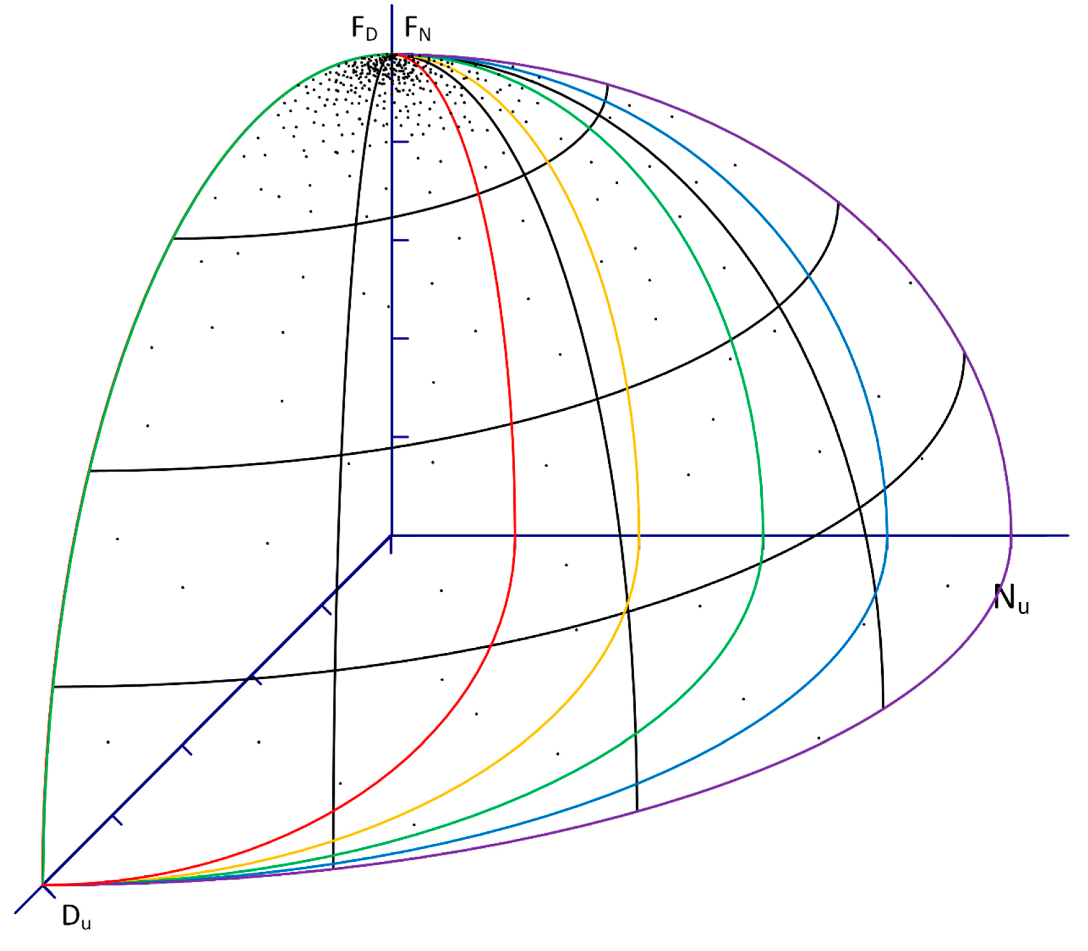
These combinations represent the scenarios for the system. In a stochastic simulation, scenarios with higher probabilities are more likely to be simulated. If the probability of A, B C, D, or E failing individually is 1% per year, then the combined probability of all five events occurring within one year is 0.015 = 1 × 10⁻⁸%, which is extremely small. The probability of just two events occurring within one year is 0.01%. In a stochastic simulation, assessing these uncommon combinations of events is very unlikely. Many years of simulation would be required to ensure each combination is simulated at least once. Further, a significant amount of simulation effort would be spent on simulations where nothing is going wrong with the system. A volumetric representation of the system’s possibility space is a useful way of demonstrating how stochastic simulation samples from within the system’s possibility space. In Figure 1, the frequency, of or more components being unavailable () is plotted against the frequency, of outage durations . Simple FN relationships are assumed and a 3-dimensional “possibility space” is created. Some of the planes of component unavailability are represented using red, orange, green, blue, and purple outlined areas. It is important to note that this possibility space is a very simplified representation of the problem—the possibility space would have several other dimensions, including possible inflows, starting reservoir elevations, as well as the length and timing of component outages. Nevertheless, using this simplified example figure, the stochastic samples can be plotted (shown as black dots). Each dot represents one sample that could be stochastically generated. The dots are centred around zero component outages, which have the highest frequency. While the samples do extend into the outer reaches of the possibility space, they provide the best coverage of the higher-frequency scenarios (zero to one components unavailable). The coverage of the less probable and more extreme scenarios where two or more components are out of service is limited.
Stochastic simulation has proven to be a very useful technique for easily and relatively quickly determining a singular estimate of the probability of dam system flow-control failure. However, there may be a significant amount of valuable information that is not being assessed in this form of the simulation model for dam safety analysis. For example, how likely is the dam to fail given a particular scenario? What is the inflow threshold that would lead to dam failure? What is the likelihood that the reservoir level for a given scenario exceeds a certain key elevation? What is the sensitivity of the simulation outcomes to the scenario impacts (outage lengths, etc.)? The stochastic simulation may not easily be able to estimate these useful parameters, which help define the criticality associated with a given scenario. The criticality of each scenario can be used to identify and rank the combinations of events being simulated, highlighting the scenarios and components with the most potential to lead to failure of the dam. There are also a wide range of possible system outcomes for a single scenario that can result from different inflows, failure impacts (outage lengths), and failure timing. Stochastic simulation may not be the most effective use of computing power if the goal is to assess a full range of the possible combinations of operating states (scenarios), and to do so in a thorough and systematic way. Determining the expected range of system behaviour in response to the complete set of “combinations of events” can help improve the understanding of system vulnerabilities.
3. Materials and Methods
Systematic analysis of each possible scenario, in theory, may be achieved using a completely deterministic simulation of predefined scenarios. However, the timing of the scenario’s predetermined adverse operating states (events) and determining whether events influence one another significantly complicates the analysis. To completely and deterministically analyze the full range of possible outcomes of a single scenario, all possible combinations of event timing and inflows should be considered. Consider an example scenario with three adverse operating states (events), A, B, and C, and 10,000 years of possible daily inflow values (this number of inflow-years is selected, in theory, to represent inflows up to and including a Probable Maximum Flood with an annual exceedance frequency of 1 in 10,000 years). There are a total of possible inflow start days. Assuming the events can happen any time within a one-year window, there are a total of possible combinations of event initiation times (the day in which the adverse operating state begins). This means possibilities for a single scenario with three events occurring. This number considers only one set of possible impacts for event A, B, and C, which may have impacts (for example, outage lengths), that can significantly vary. Clearly, the number of combinations that must be analyzed to fully define the suite of potential outcomes for a single scenario is extremely large. Additionally, there may be a very large number of scenarios to be analyzed. For a relatively simple single-dam system with two gates, a low-level sluice, and two generating units, King et al. [8] calculated that there were on the order of 1027 possible scenarios if the system was represented in significant detail. Obviously, the analysis of each scenarios its possibilities becomes computationally prohibitive, even with state-of-the-art computing technology such as cluster computing.
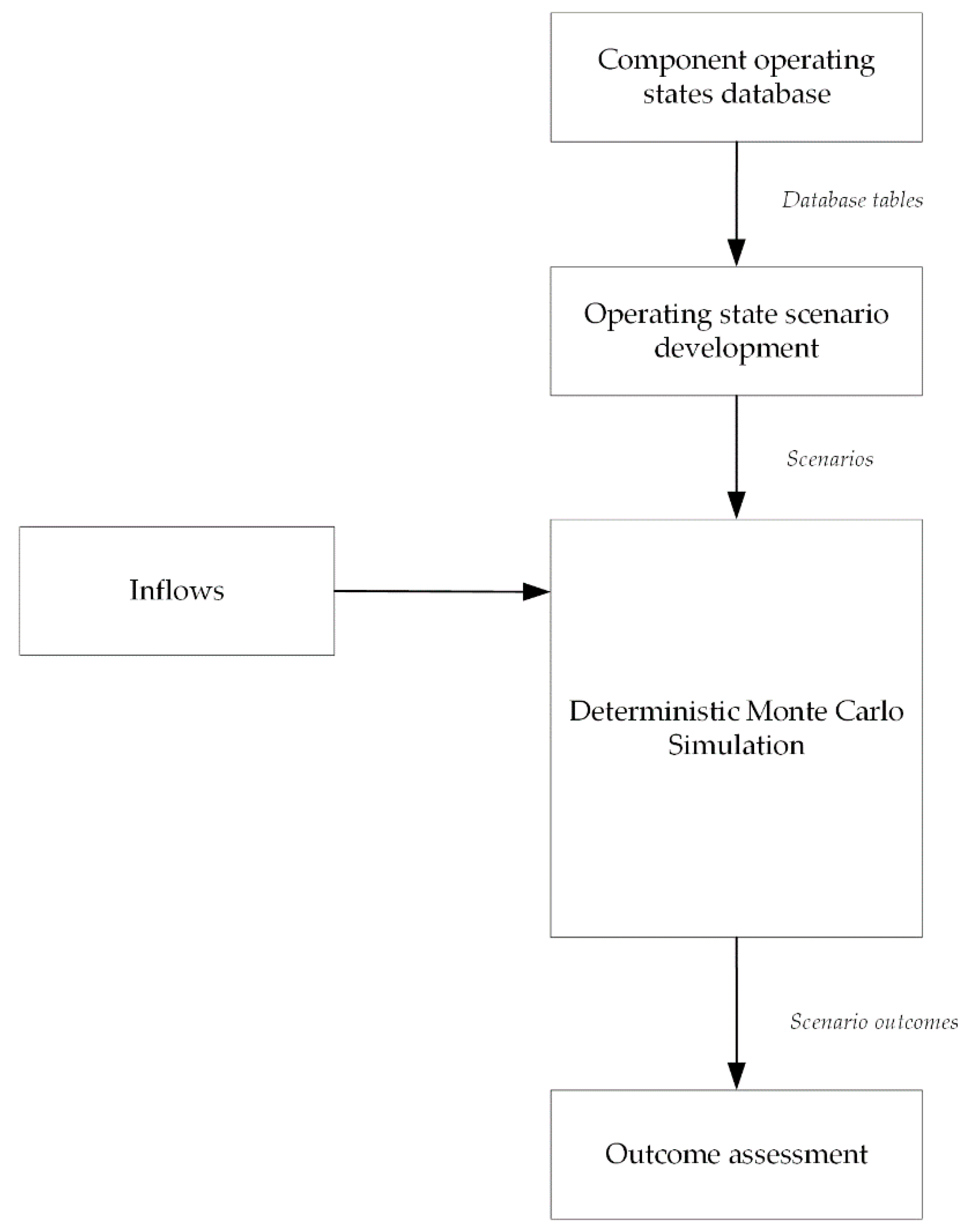
Monte Carlo selection of event timing, event impact magnitudes, and inflow start day from the synthetic record can be useful to sample a smaller number of these possibilities for each scenario and make inferences about the possible outcomes. Each predetermined scenario can be simulated through a number of Monte Carlo iterations to better understand the possible range of outcomes resulting from that scenario. This is the hybrid Deterministic Monte Carlo approach proposed in this research, where events (component operating states) are pre-selected and their impacts, timing and inflows are varied to better understand the possibilities within current computational capabilities. The approach is detailed in Figure 2. A description of the component operating states database structure, database population, and the combinatorial process for developing operating states is described in King et al. [8]. This paper describes in detail the Deterministic Monte Carlo simulation methodology, which takes the full list of combinations (scenarios) and uses simulation from within the possibility space for each scenario to estimate useful criticality parameters. An algorithm to assess the influence of preceding events on subsequent events is included within the Deterministic Monte Carlo methodology. Inflow input development is not described in this paper, but synthetic inflows can easily be generated using commonly applied stochastic techniques.
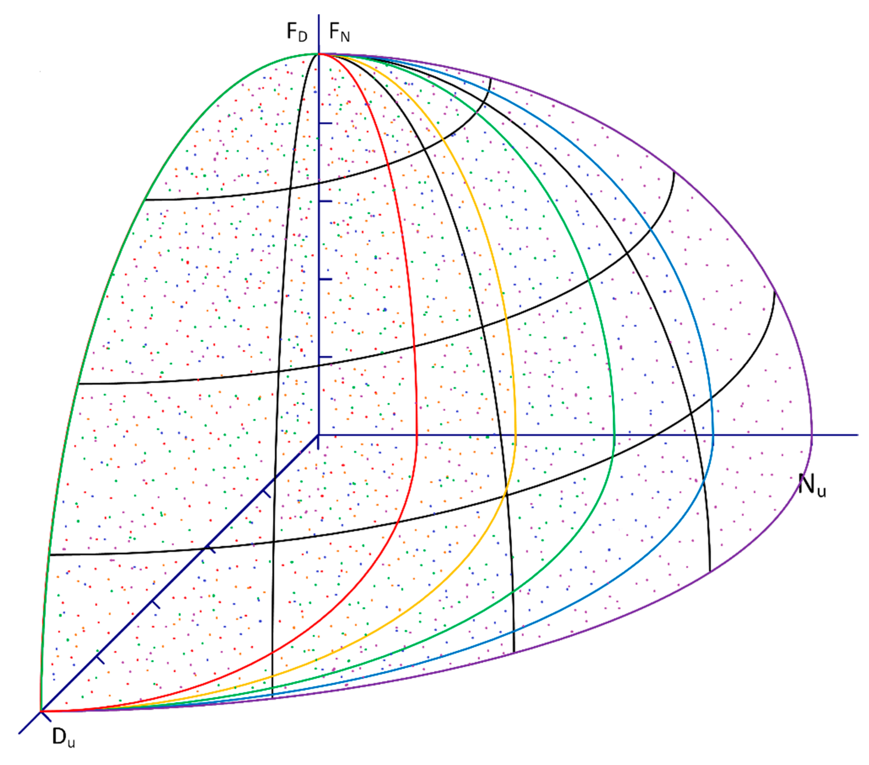
The approach presented in this paper aims to provide a more even coverage of the possibility space shown in Figure 1. This is represented in Figure 3. The sample dots are color coded, to indicate which “unavailability plane” the samples are taken from. The Deterministic Monte Carlo approach forces the simulation to take samples from within each component unavailability plane, because it does not rely on the frequencies of failure and duration to generate the samples. Each unavailability plane represents a single scenario, and the scenarios are predetermined and simulated regardless of their likelihood.
Simulation model development using system dynamics simulation, as proposed by King et al. [9], is described in the following section, which details how to develop the model to facilitate inputting of events (such as failures) and their parameters (such as the outage lengths). Next, a description of the Monte Carlo generation of simulation parameters is provided, followed by a description of the simulation process framework and event influence considerations in scenario analysis.
3.1. System Dynamics Simulation Model Development
System dynamics emerged in the 1960s through the work of Forrester [10] at the Massachusetts Institute of Technology. Forrester [10] began developing system dynamics to analyze industrial and management systems and pioneered the earliest forms of system dynamics simulation software packages. He later extended the application of system dynamics simulation to model the social dynamics of cities, countries, and the world as a whole [11,12,13]. System dynamics has since been applied across a variety of fields, including water resources engineering. Simonovic [14] presents simulation techniques that deal with water resources in general, with a particular focus on system dynamics simulation as a tool for water resources engineering. In system dynamics, a stock-and-flow model can be used to represent the system structure through feedback loops and delays. These feedbacks and delays are the source of the system behaviour. Stock-and-flow diagrams are particularly suited to showing the complex interactions between different components of the system and facilitate easy modification of the system structure to experiment with various upgrades and operations strategies that may be considered to improve system performance. Stocks are represented as boxes and flows are represented as pipelines into or out of the stock controlled by spigots (with a “source” or “sink” that supplies or drains flows). Flows may be controlled or uncontrolled. Auxiliary variables and arrows make up the other major components and these represent constants or variables that change with time according to a mathematical equation or algorithm. The dynamics of the system behaviour are a consequence of the system structure. The process for developing a model of a dam system is described in the following paragraphs.
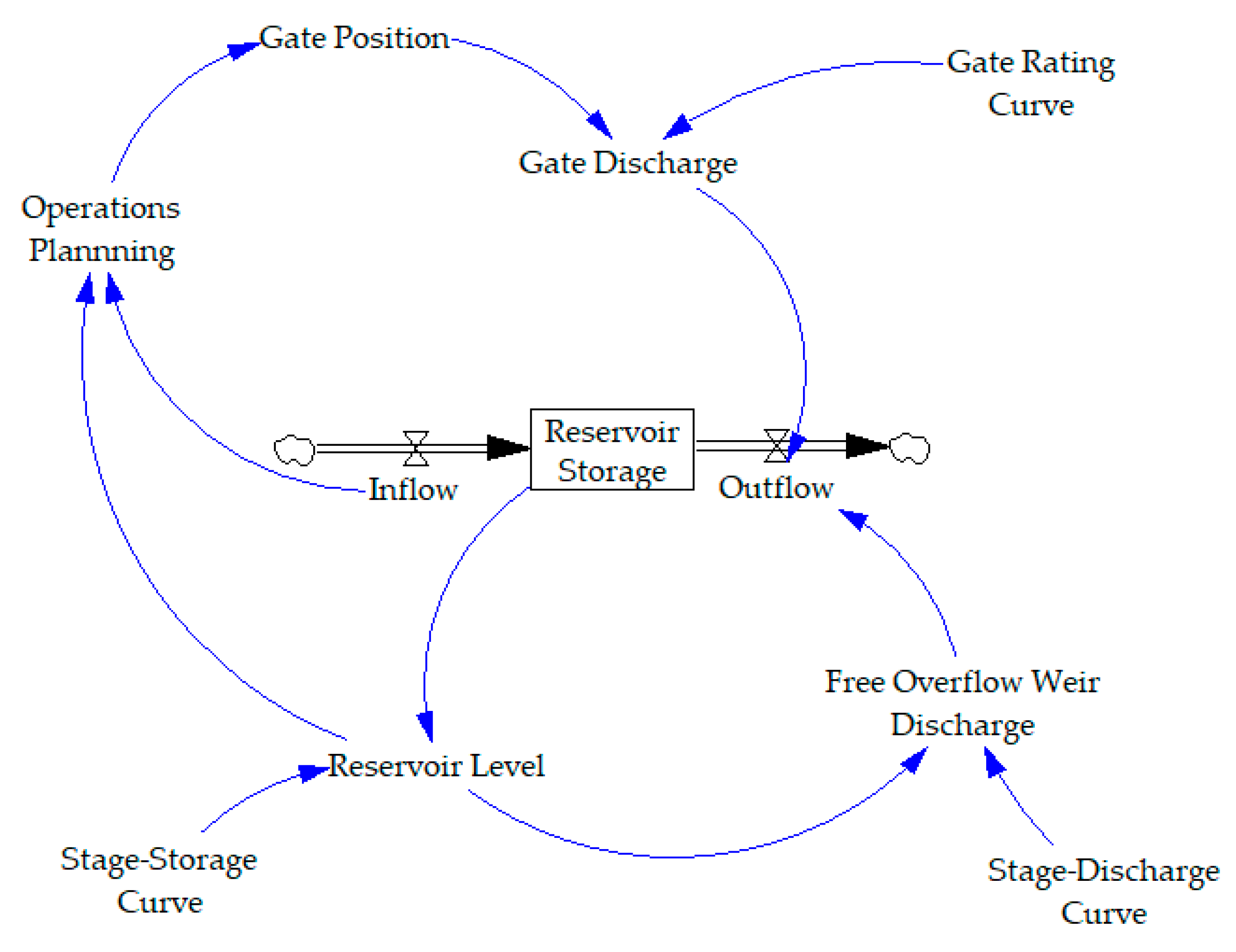
Consider a simple dam system, with a single reservoir and dam that is controlled by a free overflow weir and a gated spillway. Figure 4 contains a representation of this system.
In Figure 4, Reservoir Storage is represented as a stock with units m3. Stocks are values that accumulate or deplete over time and can only be changed by flows. Flows have the same units as the stock over time. In this example, Inflow and Outflow are the stocks and have units of m3/s. The change in Reservoir Storage can be computed as:
where represents Reservoir Storage, represents time, represents Inflows, and represents Outflows. System dynamics simulation tools use integration to calculate the value of the stock at each timestep. The Reservoir Level () value is a function of the Reservoir Storage as defined by the Stage–Storage Curve. The storage is expressed in units m3/s × day, which significantly simplifies unit conversions when working with flow rates. It is valid for reservoir elevations from El. 352.42 m to El. 388.16 m. Similarly, Free Overflow Weir Discharge () is a function of the Reservoir Level, as defined by the Stage-Discharge Curve for the weir, which has a sill of El. 378.41 m. Equations presented here are representative of an example hydropower system.
where a = −35.75057, b = 40,896.27494, c = −15,593,240.06190, and d = 1,981,715,583.08889. Note that for “flashy” reservoirs with little storage in comparison to inflow volumes, the reservoir elevation may vary greatly throughout the day, so weir discharges may also vary hourly. For a model run on a daily timestep, it may be necessary to compute the Free Overflow Weir Discharge, for a given day by iterating within the function over a 24-h period, taking into consideration fluctuations in the reservoir level. This will ensure weir discharges accurately reflect reality.
Inflows represent an external model input, which in this case, ranges from 5 to 25 m3/s. Outflows are equal to the Free Overflow Weir Discharge:
The Gate Discharge () is a function of the Gate Position () and Reservoir Level (RSE), as defined by the Gate Rating Curve. The gate rating curve can be used in a two-dimensional interpolation to determine what the corresponding flow is for a given reservoir elevation and gate position. In this example, the gate has a sill of El. 367.28 m.
Inflows may be calculated as shown in Equation (6). This inflow relationship has been selected to roughly mimic a seasonal variation.
Including some day-to-day variability in inflows for the simple system can be done using a random normally distributed variable (with a mean of 0 and a scale of 30 m3/s), which is added to the time-dependent sinusoidal inflow value. The value is then truncated, so that the minimum inflow value cannot be less than 2 m3/s. Note that this inflow variation was added for the sake of simple programming by the reader, and may not be representative of realistic variations in daily inflow values. Using historical inflows or synthetically generated inflows from the historic record are preferred for real case studies.
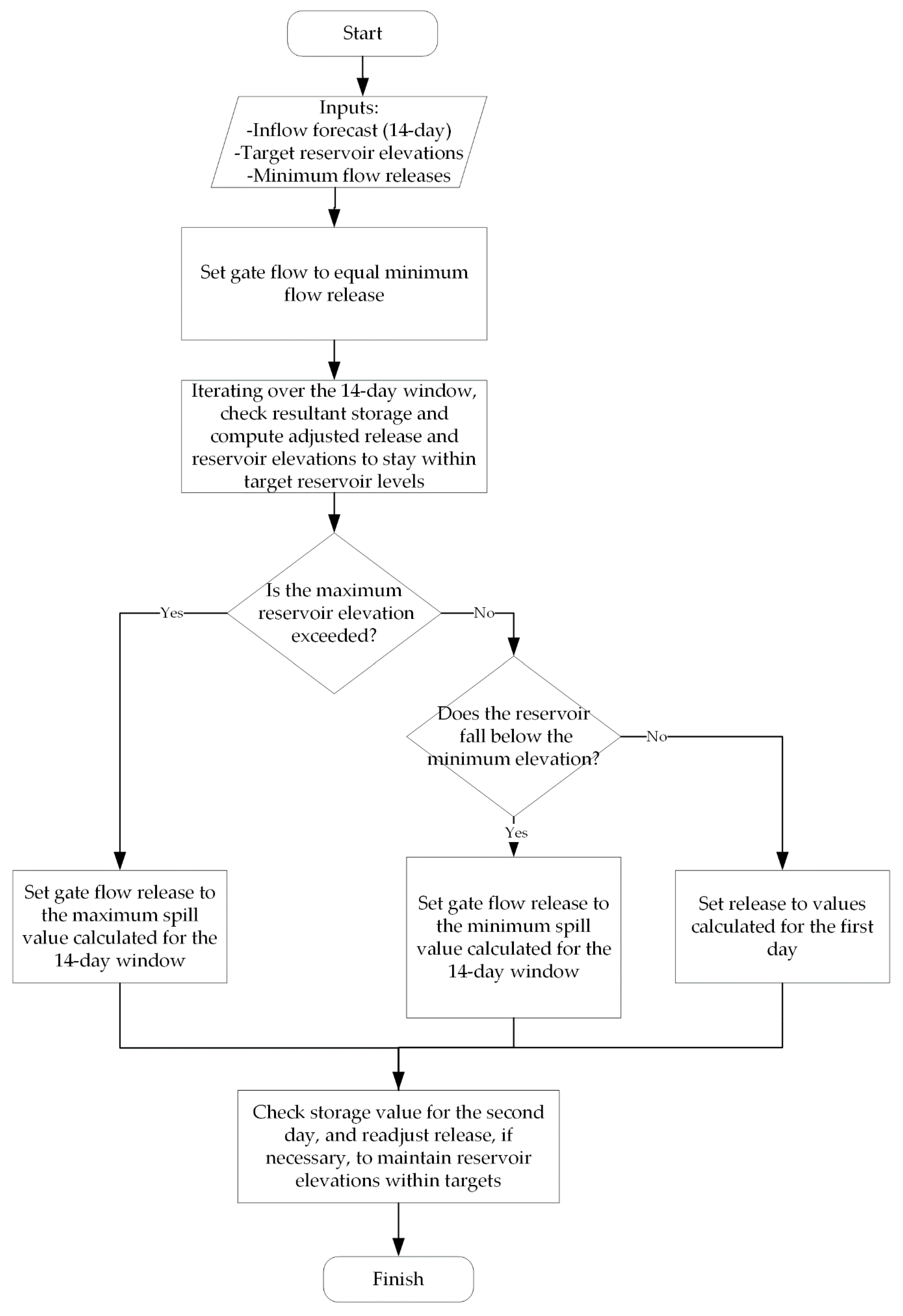
Operations planning is another key aspect of the model. Gate positions may be selected based on a number of inputs, including the inflow forecast, rule curves, target reservoir elevations, outflow constraints, and downstream impacts. Creating an algorithm to simulate operations planning is a more challenging aspect of model development, in particular in the case of cascading and parallel dam systems. Optimization is frequently cited in the literature [15,16,17,18,19] and works well for balancing inflows, downstream effects, reservoir operational limits, and outflow constraints. However, optimization may significantly impede computational efficiency, which is an important consideration when running a simulation model a large number of times. For this simplified example based on a dam system with only a single gate, a simple if-then-else type algorithm has been developed for Operations Planning (see Figure 5). The algorithm uses 14 days of inflow forecasting to determine the appropriate gate releases that will keep the reservoir level between target elevations (the normal maximum, NMax is El. 376.5 m). Inflow Forecast is based on the sinusoidal relationship described previously, with no random normal variable added. This means the operations planning algorithm has some indication of the average inflow to expect over the next 14 days but is not aware of any major deviations from the normal level due to the random normally distributed variable that is added. In a real dam system, operators may have more realistic expectations of inflow and can adjust the gate based on the hourly inflows to ensure reservoir elevations within target levels are maintained. The Operations Planning algorithm is detailed in Figure 5. The output variable from Operations Planning for this simple example is gate flow, which can be transformed into a gate position instruction. The Gate Position is calculated using a reverse two-dimensional interpolation using the Operations Planning output (the desired gate flow) and the Reservoir Level, based on the Gate Rating Curve.
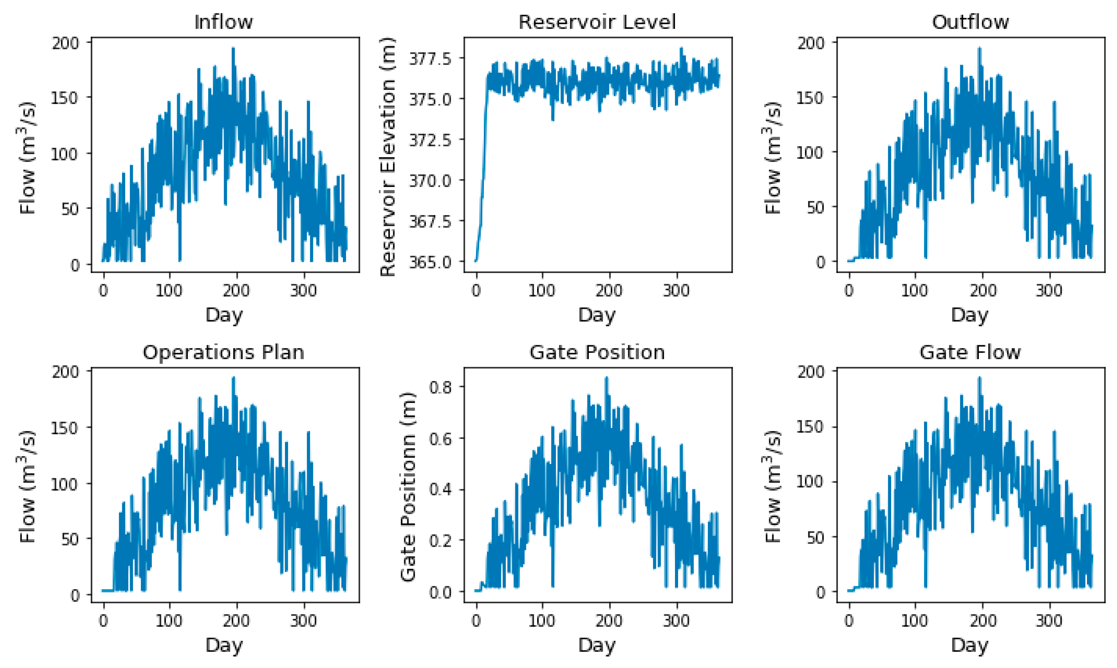
The simulation results for this simple example are shown in Figure 6. The reservoir rises to the level of El 376.5 m (the Normal Maximum Reservoir Level), and hovers at that level or just above and below based on the deviations introduced by the random normal variable added to the inflow. Note that there are no power flow release facilities included in the model, so the algorithm keeps the reservoir level high because there is no reason to discharge more additional water than necessary to meet the maximum reservoir level target. In this example, there is no free overflow spill because the reservoir stays below El. 378.41 m which is the sill of the overflow spillway. As such, reservoir inflows are roughly equivalent to reservoir outflows, operations plan, and gate flow. They are also proportional to the gate position.
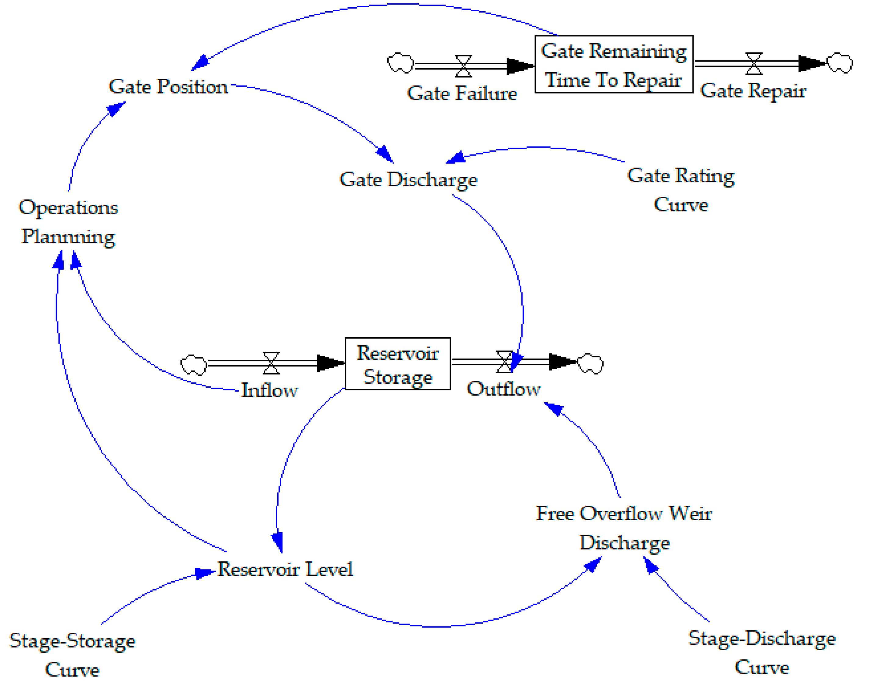
Another important feature of the simulation model within the context of this work is the ability to simulate component failures or outages. Considering the simple example developed, this can be added by creating a variable that tracks remaining time to repair following spillway operating gate failures, Gate Remaining Time to Repair, . This is modelled as a stock, which receives a pulse of Gate Failure, , when the gate fails. The stock drains with the value time when its value is positive, using the flow Gate Repair, (note, gate repair is a flow out of the stock Gate Remaining Time To Repair, and has units time; gate failure is a flow into the stock and also has units time). The gate remaining time to repair can then be implemented in the model based on the impacts of a gate outage—in this simple example, the gate fails in the closed position. Gate failure causes an inflow to the stock of 20 days at time , and the gate becomes stuck in the closed position for a 20-day period. The modified stock and flow diagram for this is shown in Figure 7.
In this example, the gate remaining time to repair is calculated as:
This formula simply implies that the gate remaining time to repair is equal to the integral of gate failure (the stock’s flow in), and gate repair (the stock’s flow out). Gate Failure is calculated as:
Gate Repair is calculated as:
The Gate Position can then be calculated based on the gate availability:
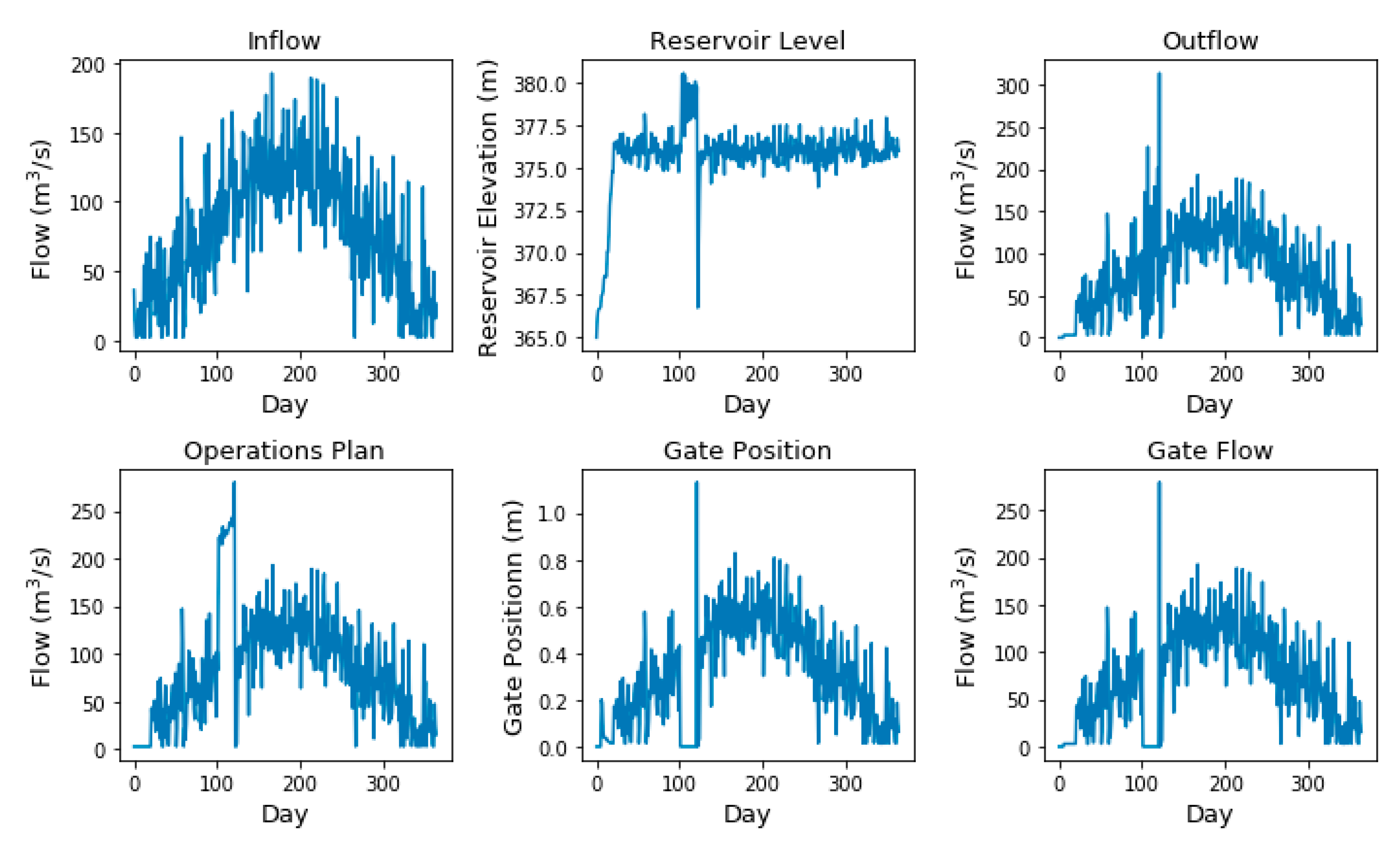
where represents the operations planning output, which is representative of the desired gate flow. Simulating this model yields the outcomes shown in Figure 8.
The impacts of the gate failure can be seen in the image starting at day 100 of the simulation, where the gate position and gate flow drop to zero, and the reservoir elevation rises above the target elevation. Flow over the free overflow weir is observed during the gate outage (these are not shown but are the difference between Outflow and Gate Flow). Once the gate is back online, the gated spillway flow is increased significantly to reduce the reservoir elevation to within the target levels. The inflow on the day of the gate’s return to service is less than predicted, so the operator opens the gate more than is necessary and the reservoir drops to just above the gate sill elevation (El. 367.28 m). In reality, operators will have a relatively better idea with respect to the expected inflow. Dam operators would also be able to adjust the gate position within the 24-h period if the inflows are less than predicted to ensure rapid drawdown of the reservoir does not occur. This is one potential limitation of running the model on a 24-h timestep, though improved inflow prediction for the operations planning algorithm would avoid the issue. For less flashy reservoirs, a daily time step may be adequate.
As the simulation model becomes increasingly complex, the non-linearity of the problem becomes more obvious. Calculation of the reservoir level response becomes increasingly more complex as additional flow release components, variable gate positions, natural variability in inflows, outages, etc., are added to the simulation model. Simulation is necessary for quantifying the dynamics of the system response to various inputs. Events happening at a lower level in the system may influence the high-level system behaviour in unpredictable ways that can be assessed through simulation.
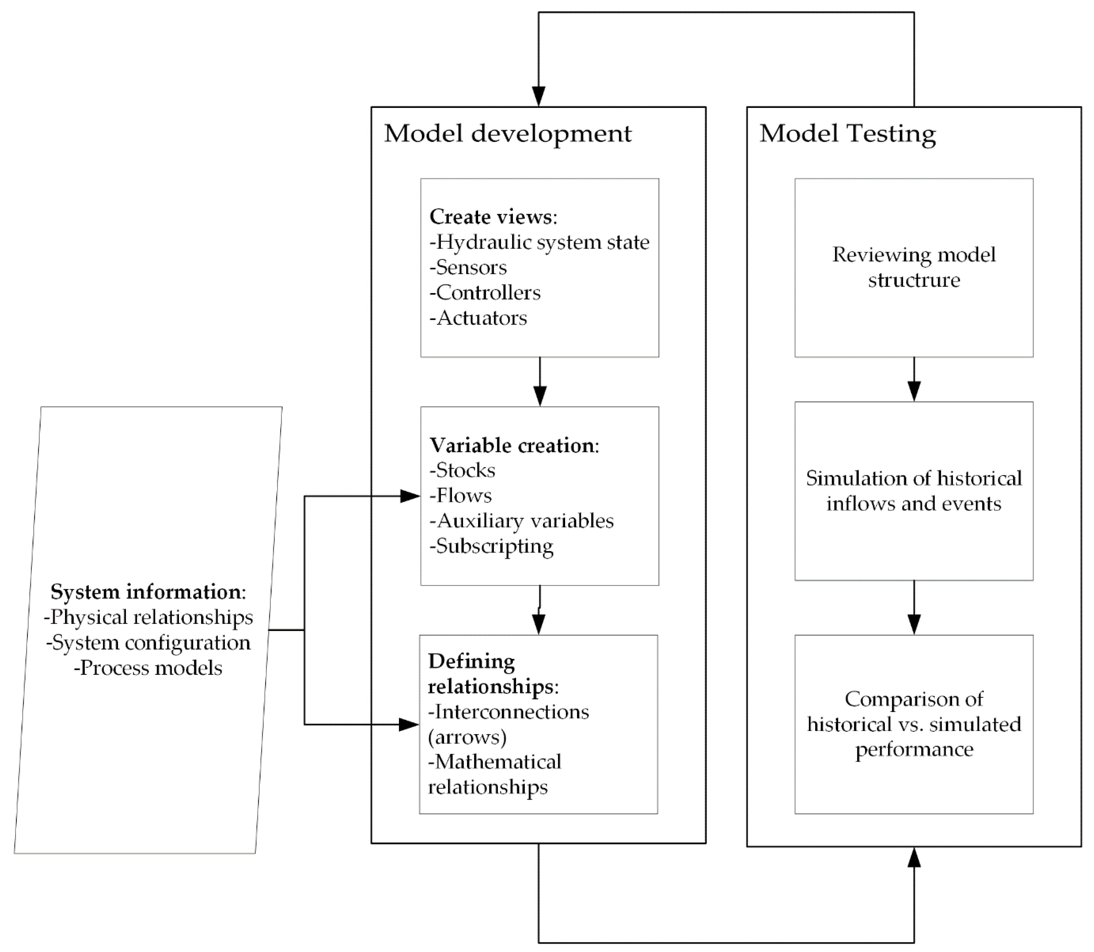
The system dynamics platform offers a particularly suitable modelling environment for complex, dynamic systems with interactions among components. The object-oriented building blocks help visualize the connections between the different components of the system. The general process for the development of a system dynamics simulation model for a dam system is described in Figure 9. A variety of different outlets and multiple dams may be added to the model depending on the system of interest. It may also be possible to represent other physical processes provided the mathematical assumptions behind them are well understood. Potentially, physical processes could include pressure transients, cavitation, uplift, earth dam seepage, and stability thresholds, though a trade-off becomes apparent between the timestep and the computational effort, since many of these phenomena may occur within minutes or seconds. This is an important area for future work.
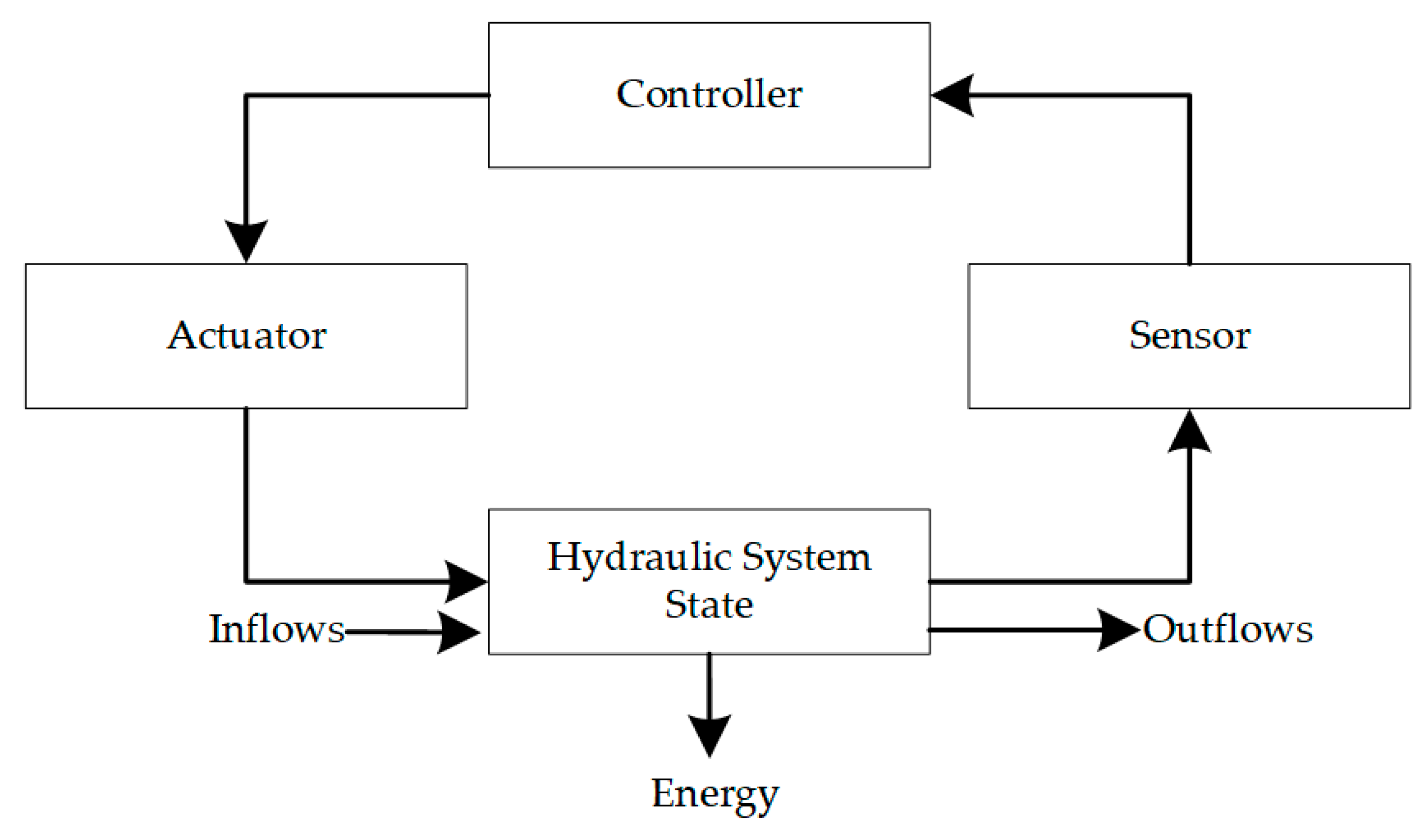
The process of model development is iterative; that is, model development is influenced by model testing, and development continues until the modeller is satisfied that the modelled system is an adequate representation of reality. The model is a description of physical and nonphysical relationships among system components. A significant amount of information about the system is required to define these relationships mathematically, and expert judgement is necessary in model development. Dividing the model into interconnected sub-systems shown in different views or sectors may be helpful. Sub-systems may be connected to each other by one or more variables. These sectors can follow a generic control loop (Figure 10) as described by Leveson [20] and adapted for a hydropower system, which includes: (1) A controller, who interprets information relating to the state of the system and produces a set of operating instructions; (2) actuators, the mechanical-electrical assemblies, which work to move gates in the controlled process; (3) a controlled process, representing the infrastructure being controlled or the hydraulic system state; (4) sensors, which relay information back to the controller; and (5) disturbances, which are not directly part of the control loop but may affect the functionality of any one of its features. This high-level system structure represents a hierarchical system of systems, with each box representing its own sub-system [20]. The benefit of developing a detailed model of the system components is that low-level failures and events within the system can be initiated and the simulation model can determine the system-level impacts for a particular set of inflows and event parameters.
Selection of the variables that will be required to adequately represent the system is another important step. The variables represent states of the system, which the modeller is interested in over time, and there may also be a number of intermediate variables that transform information between the key variables of interest. Defining the relationships requires expert knowledge of the system, data, and programming capability. Some variables equations can be represented by simple if-then-else type formulae, while others may represent non-linear relationships or even complex algorithms with a number of processes occurring internally.
The model output is only as good as the modeller’s understanding of the interactions and relationships within the system being analyzed. Like all models, simulation models are abstractions of reality. Sterman [21] argues that, because of this, all models are “wrong” and that simulation models can never be validated or verified in the traditional sense of the word. There are, however, a number of tests that can be done to gain confidence in the model performance. These tests should be done iteratively throughout the model development process. Analyzing the system structure and feedbacks to ensure all important variables are represented and their equations are grounded in reality is important. This includes checking the water balance, rating curves, and other physically derived variables. Checking the dimensions is another important model test. Historical records of system operation are also useful for testing and development of the model. A direct comparison between simulated and actual values provides information to the modeller about how well the system is mimicking reality in terms of normal operation. Comparison of historical vs. simulated reservoir levels and outflows can help the modeller adjust the system structure—this is particularly important during the development of operating rules. Once the model results are relatively close to reality, the model is ready for simulation.
3.2. Monte-Carlo Variation of Scenario Parameters
The process of King et al. [8] is used to generate scenarios, with each scenario representing a list of component operating states, which may be normal, erroneous, failed, etc., for each component in the dam system. An operating states database is presented, where the user first defines all components and their sub-components, and then their operating states, the operating state causal factors, and the operating state impacts. The database links each of the operating states to one or more causal factors and has a user-specified numeric range of impacts (minimum, maximum, and average) that can be expected should the operating state occur. Impacts may include outage length, error magnitude, or delay length. Causal factors vary depending on the system of interest and may include earthquakes, forest fires, lack of maintenance, human error, etc. The database information can be extracted in the form of tables, which contain each operating state-causal factor combination and the associated range of impacts. Linking the database information into the simulation model in a way that allows a wide range of potential outcomes to be explored for each scenario is a critical part of the implementation. An example of such a link was shown in the previous section. System dynamics modelling is inherently deterministic, so specific instructions for how to carry out the scenario must be given to the model before running. Monte-Carlo selection of simulation inputs is considered to be the most efficient way to cover as many outcomes for a single scenario as possible given computational constraints. Each scenario can be run many times, with varying simulation inputs to explore the system behavior as fully as possible without becoming computationally infeasible. This allows for some uncertainty in the outcomes to be investigated by looking at a range of potential implementations for each scenario.
Each operating state has varying impact magnitudes between minimum and maximum values specified in the database. In addition to this, the adverse operating states may be occurring within some temporal proximity to one another but not at the same time. Inflows may also significantly affect the way an operating state changes the system behaviour. While simulation facilitates the assessment of component interactions, feedbacks, and non-linear system behaviour, the Monte-Carlo variation of these important simulation inputs can help better capture a range of system behaviour that is possible as a result of a given scenario. The temporal proximity of the adverse operating states, the magnitude of impacts and the system inflows can all easily be varied using a Monte-Carlo simulation approach.
A wide range of hydrological conditions may be tested for each operating scenario, by selecting a random year and start date for each Monte-Carlo run of each scenario. The year and start date can be used to sample inflows from a synthetic inflow time series, which can be developed using a stochastic weather generator and a hydrologic model.
Operating state impacts may vary, and this is represented using minimum impact, maximum impact, and average impact (mode) as specified in the component operating states database in the operating states description. This information can be used to generate Monte-Carlo inputs with a triangular distribution [22]:
where represents a random variate from the uniform distribution between 0 and 1, represents the minimum impact value specified in the database, represents the maximum impact value specified in the database, represents the average value specified in the database and . A random impact for each operating state is generated in this way and used as the second Monte-Carlo input to the simulation model.
Timing of events may also vary within a scenario, and events can occur at the same time or within days, weeks, or even months of one another. The temporal proximity of events represents the third Monte-Carlo input to the simulation model. The causal factors for each operating state play a roll in determining operating state’s temporal proximity. The number of causal factors can be used to determine the number of time steps between adverse operating states arising from different causal factors. Operating states with the same causal factor (for example, an earthquake) are initiated at the same time. Operating states for subsequent causal factors are initiated at some value, in the future where and is equal to the number of causal factors less one (because the first causal factor is implemented at time t = 0 in the simulation). The ordering of causal factors is also varied so that the first operating state changes between Monte-Carlo inputs. For some causal factors, including lack of maintenance and aging, impact timing can be completely randomized if more than one component is affected; that is, failure of one component due to lack of maintenance may not occur at the same time as the failure of another component that has not been maintained. There may be a time limit within which these events can occur, as defined by the user for the system of interest. This is a parameter that helps increase the chance that the events are impacting one another so that the scenarios represented in the outputs are reflective of the input scenario (discussed further in the following section).
In addition to generating these randomized parameters for each scenario, it is necessary to program component-specific connections that link the database’s operating states to the specific point in the simulation model where the component failure, error, or delay occurs. An example of how this can be done was provided in the previous section. The timing and impact magnitude can be represented by variables that change with each Monte Carlo iteration. Inflow sequences can be selected from the historical record using the randomly generated day and year. Directing the impact towards the correct component and implementing it requires significant modelling effort. The implementation of these connections will differ from application to application and must be done at the front-end of the simulation model to ensure the scenario information is routed properly through the simulation model. Once the connections are made, simulation can proceed following Figure 11 as discussed in the following section.
3.3. Deterministic Monte Carlo Simulation Process
Given a large number of automatically generated combinations of events (input scenarios), and a simulation model that is set up to use the operating states and their impact parameters as inputs, scenario simulation can proceed as shown in Figure 11.
Each scenario in the scenario list (generated from the database using combinatorics) is given a unique simulation number (“seed number”) to identify it to the simulator. At the start of the simulation, a “seeds to run” list is developed. Each seed number corresponds to a line in a list of the scenarios, which contains a unique set of operating state combinations for the system. This is used to gather the information from the database tables (which contain the operating state impacts and their magnitudes) and set-up the Monte-Carlo parameters for each of the events in the scenario to be simulated. The Monte Carlo parameters are randomized inputs that vary within the bounds specified in the operating states database. This allows for a more complete exploration of the potential outcomes for a given scenario. Once the Monte Carlo input generation is completed based on the scenario of interest, the simulation of the scenario proceeds.
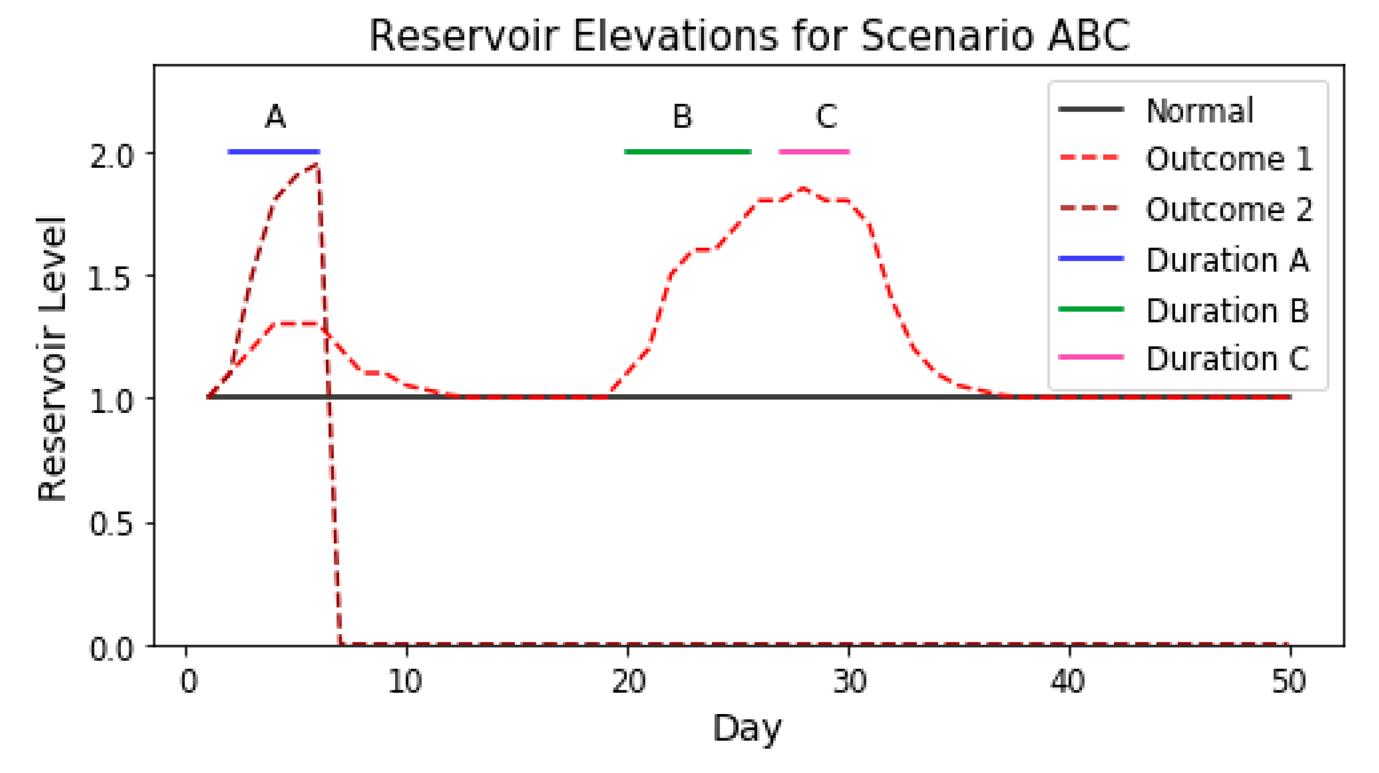
Following the simulation of each scenario iteration, timing considerations must be addressed, to ensure the results are accurately attributed to the scenario being represented. It is important to address the issue of whether preceding events are influencing the results of subsequent events. Such considerations arise when a component failure has been rectified, but the overall system remains in a “disturbed state”; that is, the system has not been restored to the state that it would have been in if the component failure had not occurred. The “system state deviation” needs to be considered along with the timing of component failures. This can be achieved by analyzing whether the reservoir level has returned to a predefined “normal” state following the initiation of an event. If not, there may be independent sub-scenarios within the simulation that should not count towards results of the scenario being analyzed. Consider the example shown in Figure 12, which has three events, A, B, and C occurring within some time of one another.
In the example, the reservoir has a constant elevation of 1 m under normal circumstances (everything being operational). For Outcome 1 (light red), Event A causes an increase to about 1.3 m and then the reservoir level returns to the normal elevation of 1 m prior to the initiation of Event B (this is determined by an operations planning algorithm within the simulation model). Event B causes in increase in reservoir elevation to about 1.8 m, after which Event C begins and increases the reservoir a further 0.1 m. After Event C, the reservoir returns to its normal elevation as a result of the operations planning decisions. In Outcome 1, Event A does not have any impact on the outcome of Events B and C, because the reservoir level has returned to a normal elevation. Event B, however, does impact Event C. Thus, for Outcome 1, two scenario results are shown: (1) The result of Event A, and (2) the combined result of Events B and C. In Outcome 2 (dark red), the reservoir rises to about 1.95 m following Event A, at which point dam breach is triggered and the reservoir drops to 0 m in elevation. In this case, the only real scenario being analyzed is Event A. This example shows that despite the simulation being intended to analyze the combined impacts of Events A, B, and C, they cannot be assumed to be influencing one another. Some analysis of each simulated outcome (the reservoir levels from each simulated Monte-Carlo iteration) is required to ensure simulation results are attributed to the actual scenarios being represented within the analysis.
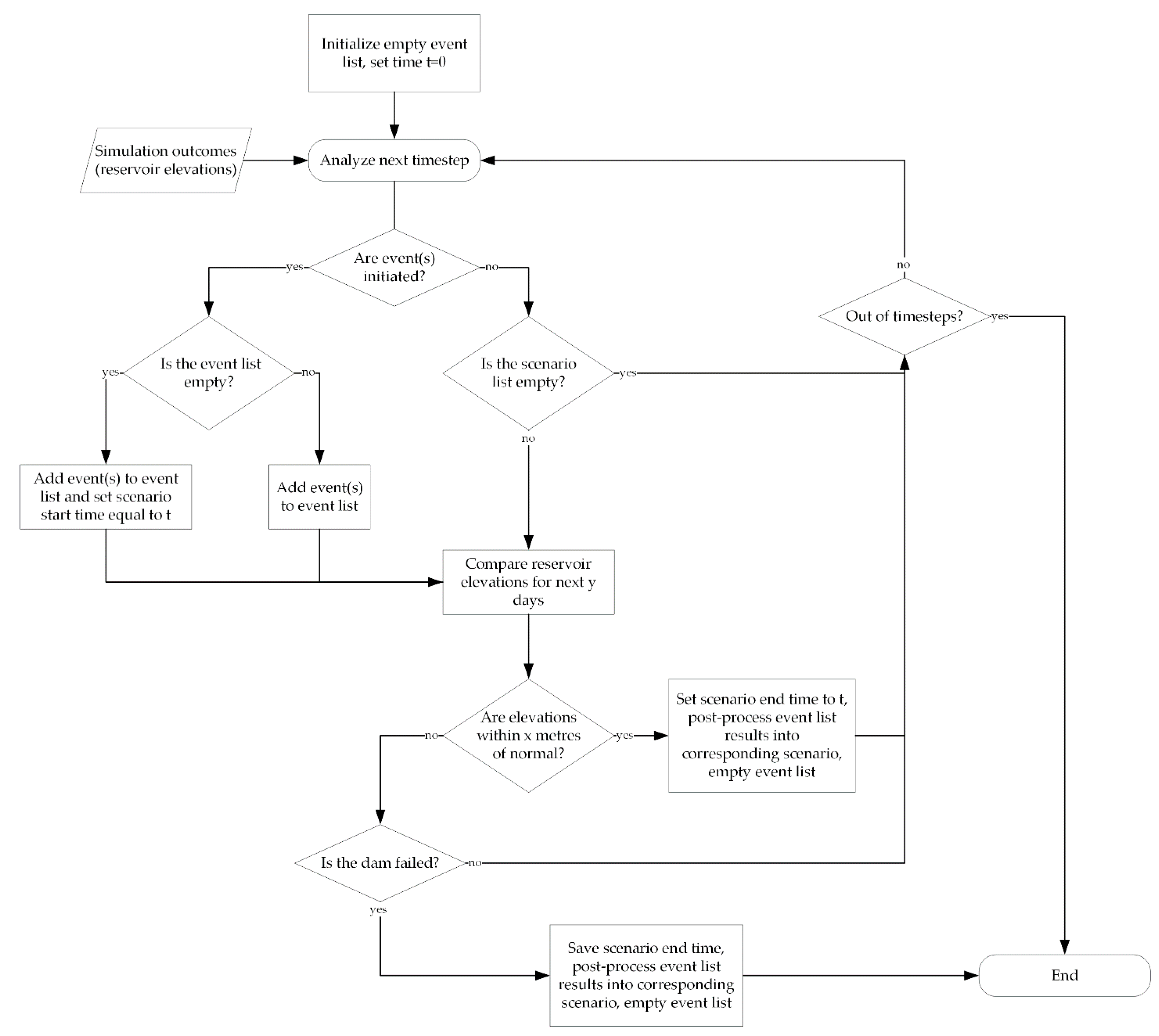
Assessing the event dependency can be done by analyzing the “system state deviance” to determine whether subsequent events are dependant on preceding events. An event dependency algorithm to analyze the outputs from each iteration is necessary in order to count the simulation results towards the scenarios that are truly represented within the output data. Given the time of occurrence of A, B, and C, the reservoir level under normal operations, and the resultant reservoir levels, a simple comparison can be used to determine whether events are influencing one another. The algorithm to analyze simulation outcomes from a single iteration is shown in Figure 13.
First, an empty event list is created, and the time is set to . The analysis starts by first checking if a new event is initiated at the current time step (the event initiation time is determined through the Monte-Carlo sampling). If so, the event is added to the event list. If no previous events are in the list, time t represents the scenario start day. If there are events in the event list, a check is done to see whether the event impacts are over—this is a simple comparison of the following y days of simulated reservoir elevations with the previously expected reservoir elevations for that set of inflows. The choice of the number of subsequent days to be compared, y, depends on the system being modelled and may be shorter or longer depending on the storage relative to the inflows. If the elevations are within a certain threshold, , of the previously expected reservoir levels for all days within days of the current day, the scenario is considered to be over. The threshold is a small number that indicates the reservoir levels are basically the same—it may also vary depending on the reservoir being modelled and must be chosen by the analyst for the system of interest. Once the reservoir levels are restored to the previously expected values, the results for the scenario are saved, the event list is emptied, and the analysis proceeds to the next timestep. If the elevations are not yet matching, the analysis proceeds to the next time step, as long as the reservoir elevations have not risen to a sufficient level to fail the dam by overtopping. If the dam has failed, the results are processed and saved for the events in the list. The process continues through all of the timesteps, until either there are no more time steps to analyze or the dam has failed.
This process, when applied to Outcome 1 in Figure 12, saves results for Scenario A and Scenario BC. For Outcome 2, it saves results for Scenario A only. This process could also be useful to analyze outcomes from fully stochastic simulation models, extracting more information than a singular probability of failure for the system being analyzed.
Once all iterations for a given scenario are analyzed, the scenario results are saved and the seed number is added to the completed seeds list. Then, a new scenario is chosen from the seeds to run list and executed. Simulation of the complete list of scenarios is a significant computational task, depending on the size of the scenario list and complexity of the simulation model. Linking of each individual component in the database to the corresponding system dynamics model component is required prior to the start of the simulation.
In using the Deterministic Monte Carlo approach, it is important to consider that the goal of the exercise is to analyze all scenarios (predefined combinations of operating states) as completely as possible given computational time constraints, to determine the criticality of these combinations. There should be enough data on each scenario to estimate the range of expected system performance and calculate the criticality parameters: Conditional failure frequencies, failure inflow thresholds, and conditional reservoir level exceedance frequencies. To ensure there is enough data collected for each scenario, it may be necessary to limit the time between events to ensure their collective impacts can be assessed. This limit may be determined as a function of the impact lengths for a given iteration (for example, by taking the sum of impact lengths). Whether the event initiation time limit should be greater than or less than the sum of the impact lengths requires experimenting with scenarios to determine how long the system typically takes to return to normal operation. For “flashy” reservoirs with relatively limited storage compared to inflows, the recovery time following a return to normal operations may be quite short—days or even hours. For reservoirs with large storage in comparison to inflows, this recovery time may be significantly longer. The recovery time may also be less than the sum of impact lengths, due to inflows that are less than the total capacity of the available flow conveyance facilities. The recovery time should influence the modellers decision regarding the appropriate time limit for event initiation. If the time limit for event initiation is too long, there may be two or more sub-scenarios within each scenario, and not enough data relating to the collective impact of the combination of events.
4. Results
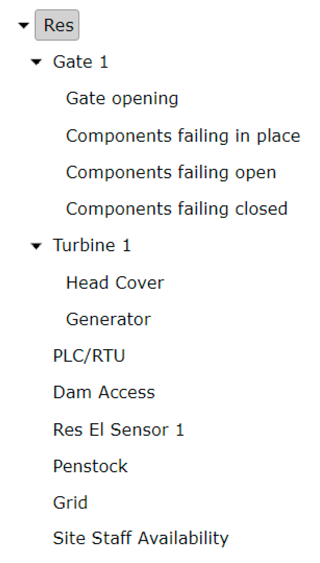
To demonstrate the utility of the simulation framework presented in this research, an example scenario outcome is shown. The case study is based on a single dam with a single spillway operating gate with a capacity of 1100 m3/s at the maximum normal reservoir level, and a gate sill of El. 367.28 m. The gate rating curve is included in the Appendix. The dam also has a single turbine with a discharge capacity of 65 m3/s and an intake sill of El. 352.96 m. The turbine is operated remotely, and the gate may be operated either remotely or manually by site staff. The system was also assumed to have a free-overflow section of the Concrete Dam capable of discharging approximately 255 m3/s prior to the initiation of dangerous dam overtopping flows. The overflow spillway sill is at El. 380.41 m (the elevation of the Concrete Dam) and its rating curve is shown in the Appendix. Reservoir level operating ranges for the case study include a water-licensed full supply of the reservoir at El. 377.95 m above sea level (WL Max.) and a preferred minimum operating level at El. 367.5 m (NMin). A preferred high reservoir level of El. 376.5 m is targeted (NMax), with some excursions above this permitted for shor-term flood control. For the spillway gates, relationships were assumed between gate opening, reservoir level, and discharge (See supplementary materials Table S2). A relationship is also assumed between reservoir level and storage. These relationships can be found in the supplementary materials File S1. The dam is assumed to fail above reservoir levels of El. 381.73 m. The components list for the system is shown in Figure 14. A more detailed description of the components, their operating states, and impacts is provided in Supplementary materials File S1.
A simulation model of a hydropower system, described in detail in by King et al. [9], was adapted for this case study with simplified components shown in Figure 14. The component interactions are represented through feedback loops that determine the system behavior. This complex representation of the system structure allows the modeler to implement low-level failures within the simulation to determine the system-level impacts. More information about the simulation model setup can be found in the Appendix, which also contains the database setup for the simulation. The Deterministic Monte Carlo approach was used to evaluate 552,960 scenarios, each for 2000 iterations. Each scenario was run for one year, for a total of 1.1 billion simulated inflow-years. The complete results from the full simulation are included in the Supplementary Materials Table S1.
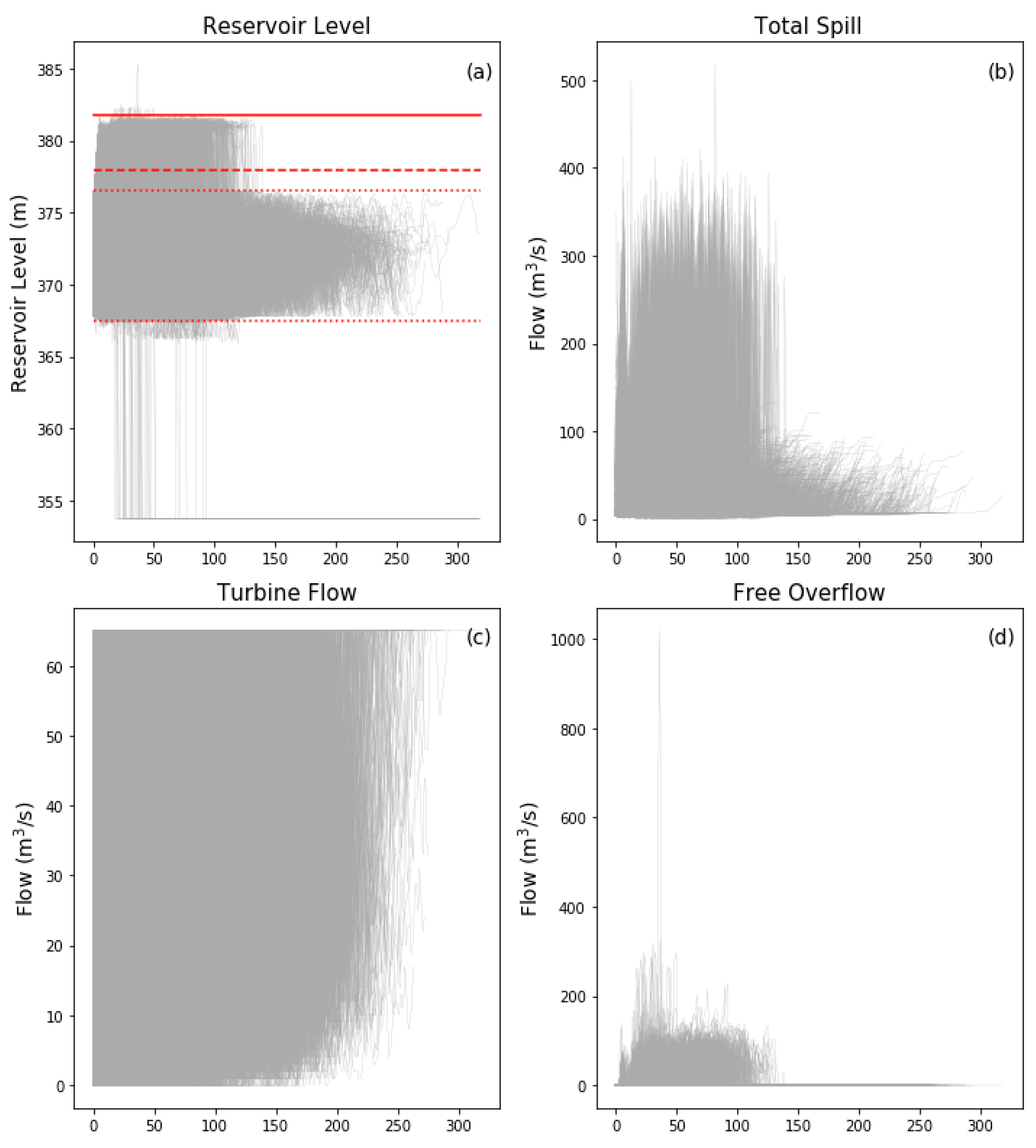
For a more concise description of the Deterministic Monte Carlo outcomes, a single scenario is shown here, which involves the failure of a component of the gate system that results in the gate being stuck in place, a power grid outage, and a site access delay. This is one potential combination of events, which may together be uncommon but individually may occur more frequently. The system is structured such that if the power grid is non-functional, gate operation must be carried out remotely, which requires access to the dam site to operate the gate. Unavailability of the power grid also leads to a forced outage of the generating unit. Ten thousand Monte Carlo iterations of this scenario are analyzed. The time within which the events can happen is limited by the duration of the events. In total, 8842 out of the 10,000 iterations had all events influencing one another. In the remaining scenarios, the events either did not influence one another or the dam failed prior to the initiation of subsequent events. The results from this sub-set of iterations are shown in Figure 15. The complete set of results can be found in the supplementary materials Table S3—this data contains the full 10,000 years, which were simulated for 365 days. The python output file for this scenario can be found in the supplementary materials File S2, which contains python arrays of each output. The grey lines in Figure 15 contain the results for each of the 8842 iterations where all three events occurred and affected one another. Each line is plotted from the start to the end of the scenario. The maximum scenario length was 310 days, so all lines truncate either on or before this value. It is important to note that the simulation model randomly selects an inflow start date between 1 January and 31 December from the inflow time-series. Inflows represent a synthetic dataset, which can be created through the use of a weather generator [23] and hydrologic model [24]. Inflow development is discussed further in the Appendix. Because the inflow start days vary, the figures may not appear to have a seasonal trend, since the plots begin at day one of the scenario, regardless of the day and year of the synthetic inflow on day one. This means that 4 April could be modelled alongside 30 January, and results in a lack of seasonal trend. The reason for this is so that the range of impacts for the scenario can be illustrated by plotting scenario results alongside one another (disturbed system states occurring concurrently). Figure 15a shows the reservoir levels, with the dotted red lines illustrating the preferred operating range, the dashed line showing the water licensed maximum, and the solid red line showing the reservoir level above which dam breach is initiated. It is clear from the plot that in a number of the scenarios, the reservoir elevations exceeded the key levels, with 48 of 8842 iterations exceeding the breach threshold. The statistics relating to conditional frequencies of failure and reservoir level exceedance are shown in Table 1. In Figure 15b, the spill releases are plotted. The values vary over time and have a maximum of about 500 m3/s. Figure 15c shows the turbine flow releases, which vary between 0 and the maximum of 65 m3/s. Figure 15d shows the overflow, which varies to a maximum of about 1000 m3/s.
Analyzing these results can help determine key criticality parameters for the scenario being modelled. Table 2 shows these parameters. The conditional failure frequency for this scenario is 0.54 percent, which is the proportion of failures that occurred (48) over the number of iterations considered (8842). This is the conditional failure frequency, assuming all three events have occurred and affected one another, and does not represent the overall failure rate for the system. Two inflow thresholds are calculated: The first one is equal to 175 m3/s, which represents the smallest of 48 maximum daily inflows in the 5 days preceding failure. The second inflow threshold is equal to 144 m3/s, which represents the smallest of 48 average daily inflows in the five days preceding failure. Finally, three conditional frequencies of exceeding key reservoir elevations are calculated. The conditional frequency of exceeding El. 376.5 m is 50.2%, and the conditional frequency of exceeding El. 377.95 m is 37.3%. The conditional frequency of overtopping the concrete dam (exceeding El. 380.41 m) is 21.6%—this means there could be significant damage to infrastructure at the dam site in 21.6% of the simulated scenarios. The parameters selected are considered to be useful indicators of a scenario’s criticality. When compared alongside values for other scenarios, these parameters can help rank the most severe of the simulated scenarios and can be useful in identifying vulnerabilities within the system.
Simulation of the complete list of scenarios (combinations of events) for the simplified system would generate failure frequencies for each of the scenarios as shown in Table 2. When combined with the probability of occurrence of the events, an overall estimate for the probability of flow-control failure for the system can be made using basic concepts from probability theory. A simple example is used to demonstrate this. Consider a system with components A, B, and C, which are each functional or failed. If each of the three components has lower and upper bound failure rate estimates ranging from 0.1% to 1%, an overall probabilistic assessment of the system can be made using the failure frequencies generated through Deterministic Monte Carlo simulation, as shown in Table 2. The conditional failure frequencies are assumed for the sake of the example.
In Table 2, the conditional frequency of system failure (observed failure frequency per year) is multiplied by the probabilities of the system states, as follows: where , and the solid line over the component indicates it is not failed, and represents the conditional probability of failure for the system given the scenario has occurred. In the table, the lower and upper bound estimates are calculated to illustrate the sensitivity of the results to the assumed component failure probabilities. This is particularly advantageous where failure rate data are limited and uncertain. The Deterministic Monte Carlo approach does not require complete re-simulation if the sensitivity of the results to the assumed probabilities is to be analyzed. The sensitivity of the overall probability of failure for the system can be easily calculated by simply modifying the assumed component failure rates and updating the equation. It is important to note the common-cause failures may require a more complex approach to computation of the overall likelihood of failure, though there is some guidance on this within the literature on Event Tree Analysis [25].
5. Discussion
This research details a new simulation framework for systematic and dynamic analysis of combinations of events (scenarios) that can occur during dam system operation. Combinations of events are determined using an automated process that calculates the Cartesian Product of component operating state sets from a database of operating states. The Deterministic Monte Carlo framework uses system dynamics simulation, with Monte Carlo inputs that vary the scenario parameters (event timing, event impact magnitude, and inflows). The system dynamics simulation model represents interactions among a hierarchical system-of-systems, where events can be initiated within a low-level of the system to determine the resulting system behavior, including the value of the reservoir level over time. The process for developing and testing a simulation model is described as well as the Monte Carlo inputs. The simulation framework to systematically evaluate each of the pre-determined combinations of events is presented. While only a small portion of the scenario’s possibility space can be explored given computational limitations, the Deterministic Monte Carlo approach does not rely on probabilities, and thus gives a more even coverage of the possibility space than is possible using stochastic simulation. The Monte Carlo iterations for each scenario provide information that can be used to estimate the criticality of each scenario, which is not possible using stochastic simulation. The criticality parameters selected include the conditional probability of failure, the failure inflow thresholds, and the conditional probability of reservoir level exceedance.
A simple case study is presented. A complete simulation of 552,960 scenarios, each with 2000 iterations, was performed and is outlined in the Appendix. The criticality parameters from each scenario are included in the Supplementary Materials Table S1. The results from a single scenario are presented to illustrate how the approach presented in this research can more thoroughly analyze the dynamic system response to a scenario, as well as the scenario’s criticality. In the example scenario, the gate fails in place, the grid fails, and site access is delayed. Of 10,000 simulated iterations of the scenario, 8842 of these were true representations of the scenario, where all three events occurred and influenced one another. In the remaining 1158 scenarios, the reservoir level either returned to normal prior to the initiation of subsequent events, or the dam failed before all three events were initiated. Results from the 8842 scenario were plotted and criticality parameters were computed. A simple example showing how results could be used to estimate overall probabilities of failure for the system (and their uncertainty) is also shown.
The approach presented in this work uses the criticality parameters to assess how likely the dam is to fail by overtopping given a particular scenario has occurred, what the inflow thresholds that can lead to overtopping failure are, as well as the likelihood that the reservoir level for a given scenario exceeds a certain key elevation. Determining the sensitivity of simulation outcomes to the scenario impacts (outage lengths, etc.) is done through varying the impacts using Monte Carlo techniques.
This approach can provide useful insights about the vulnerability of the system to a wide range of scenarios. Components that may not be considered by dam owners to be dam safety critical may emerge as significant contributors to failure as a result of this analysis. Identifying these vulnerable components can help dam owners better manage, update, and maintain their assets to avoid potentially unsafe conditions. The results of the analysis may also be useful for developing emergency response strategies and planning outage timing for upgrades and maintenance. If the probabilities of the events are known, simulation results can also be used to estimate the probability of overtopping failure for a dam system, taking into account a more thoroughly analyzed range of possible operating scenarios than may be simulated using a fully stochastic framework. Sensitivity analysis of the computed overall probability of overtopping failure to the assumed component probabilities is straightforward and does not requires significant computational effort. This is particularly useful in the absence of reliable data relating to the probability of failure of various components of the system. Using more commonly applied stochastic techniques, complete re-simulation would be required to assess the sensitivity of the overall result to changes in the event probability assumptions.
Ultimately, the choice of analyzing the dynamic system response to disturbances using stochastic or Deterministic Monte Carlo simulation depends on the end goal. Stochastic simulation is a relatively efficient means of estimating a singular value for the probability of failure for a dam system and is capable of analyzing the dynamic system response to various events that may occur. The Deterministic Monte Carlo approach requires significantly more computational effort but is able to cover more thoroughly the possibility space within which the system may be required to operate over its lifetime. This improved coverage of the possibility space can help determine the most critical combinations of events—events that may individually appear to be benign, but when combined, may have potentially disastrous consequences. Ultimately, a trade-off exists between the computational time requirement and the level of complexity that can be modelled using this approach. With advances in computational power, the Deterministic Monte Carlo approach may be suitable for analysis of real dam systems in a significant level of detail.
In the future, it may be desirable to incorporate additional methods of dam failure into the simulation. These include dam instability as a result of uplift or sliding, cavitation, surficial erosion, slope instability, pressure transients, and perhaps internal erosion. Programming these potential effects into the model may be possible if the dynamics of the physical phenomena are well understood. In the case of cavitation and pressure transients, there may be significant additional computational effort required to adequately model these processes, since they occur at a very fine time step (while the model may be run at a daily time step to reduce computation time). Experimenting with incorporating these physical processes into the model is an important area for future work and would significantly improve the ability of this approach to capture a wide range of possible system behavior.
Supplementary Materials
The following are available online at https://www.mdpi.com/2073-4441/12/2/505/s1: Table S1: Criticality parameters for all 552,960 scenarios “S1.xlsx”, Table S2: Gate rating curve for the case study example “S2.xlsx”, Table S3: Case study scenario results spreadsheet for all 10,000 iterations “S3.xlsx”, File S1: Additional information pertaining to the case study “S1.pdf”, and File S2: Scenario results arrays which can be read in python “S2.npz”.
Author Contributions
Conceptualization, L.M.K. and S.P.S.; methodology, L.M.K.; software, L.M.K.; formal analysis, L.M.K.; writing—original draft preparation, L.M.K.; writing—review and editing, S.P.S.; visualization, L.M.K.; supervision, S.P.S.; project administration, S.P.S.; funding acquisition, S.P.S. All authors have read and agreed to the published version of the manuscript.
Funding
This research was funded by the Natural Sciences and Engineering Research Council of Canada, Collaborative Research and Development grant number 462879-2013, with support from BC Hydro.
Acknowledgments
The authors would like to acknowledge Des Hartford of BC Hydro for his valuable insights and collaboration on the research. Thanks also to Derek Sakamoto of BC Hydro who provided additional input throughout the research project.
Conflicts of Interest
The authors declare no conflict of interest.
References
- Regan, P.J. Dams as systems—A holistic approach to dam safety. In Proceedings of the USSD Annual Meeting and Conference, Sacramento, CA, USA, 12–16 April 2010; pp. 554–563. [Google Scholar]
- Alfaro, L.D.; Baecher, G.B.; Guerra, F.; Patev, R.C. Assessing and managing natural risks at the Panama Canal. In Proceedings of the 12th International Conference on Applications of Statistics and Probability in Civil Engineering, ICASP12, Vancouver, BC, Canada, 12–15 July 2015; pp. 1–8. [Google Scholar]
- Hartford, D.N.D.; Baecher, G.B.; Zielinski, P.A.; Patev, R.C.; Ascila, R.; Rytters, K. Operational Safety of Dams and Reservoirs; ICE Publishing: London, UK, 2016. [Google Scholar]
- Komey, A.; Deng, Q.; Baecher, G.B.; Zielinski, P.A.; Atkinson, T. Systems Reliability of Flow Control in Dam Safety. In Proceedings of the 12th International Conference on Application of Statistics and Probability in Civil Engineering, ICASP12, Vancouver, BC, Canada, 12–15 July 2015; pp. 1–8. [Google Scholar]
- Baecher, G.; Ascila, R.; Hartford, D.N.D. Hydropower and Dam Safety. In Proceedings of the STAMP/STPA Workshop, Cambridge, MA, USA, 2013; Available online: http://psas.scripts.mit.edu/home/wp-content/uploads/2013/04/03_Baecher_STAMPWorkshop2013c.pdf (accessed on 7 February 2020).
- Komey, A. A Systems Reliability Approach to Flow Control in Dam Safety Risk Analysis. Ph.D. Thesis, University of Maryland, College Park, MD, USA, 2014. [Google Scholar]
- El-Awady, A. Probabilistic Failure Analysis of Complex Systems with Case Studies in Nuclear and Hydropower Industries. Ph.D. Thesis, University of Waterloo, Waterloo, ON, Canada, 2019. [Google Scholar]
- King, L.M.; Schardong, A.; Simonovic, S.P. A combinatorial procedure to determine the full range of potential operating scenarios for a dam system. Water Resour. Manag. 2019, 33, 1451–1466. [Google Scholar]
- King, L.M.; Simonovic, S.P.; Hartford, D.N.D. Using system dynamics simulation for assessment of hydropower system safety. Water Resour. Res. 2017, 53, 7148–7174. [Google Scholar] [CrossRef]
- Forrester, J.W. Industrial Dynamics; MIT Press: Cambridge, MA, USA, 1961. [Google Scholar]
- Forrester, J. Urban Dynamics; MIT Press: Cambridge, MA, USA, 1969. [Google Scholar]
- Forrester, J.W. World Dyamics; Wright-Allen Press: Cambridge, MA, USA, 1971; p. 145. [Google Scholar]
- Forrester, J.W. The beginings of System Dynamics. In Proceedings of the International Meeting of the System Dynamics Society, Stuttgart, Germany, 10–14 July 1989; pp. 1–16. [Google Scholar]
- Simonovic, S.P. Managing Water Resources; UNESCO: London, UK, 2009. [Google Scholar]
- Scipy Developers Interpolation (scipy.interpolate). Available online: https://docs.scipy.org/doc/scipy/reference/tutorial/interpolate.html (accessed on 30 November 2019).
- Storn, R.; Price, K. Differential Evolution—A Simple and Efficient Heuristic for Global Optimization over Continuous Spaces. J. Glob. Optim. 1997, 11, 341–359. [Google Scholar] [CrossRef]
- Reddy, M.J.; Kumar, D.N. Optimal reservoir operation using multi-objective evolutionary algorithm. Water Resour. Manag. 2006, 20, 861–878. [Google Scholar] [CrossRef] [Green Version]
- Che, D.; Mays, L.W. Development of an Optimization/ Simulation Model for Real-Time Flood Control Operation of River-Reservoirs Systems. Water Resour. Manag. 2015, 29, 3987–4005. [Google Scholar] [CrossRef]
- Fayaed, S.S.; El-Shafie, A.; Jaafar, O. Reservoir-system simulation and optimization techniques. Stoch. Environ. Res. Risk Assess. 2013, 27, 1751–1772. [Google Scholar] [CrossRef]
- Leveson, N.G. Engineering a Safer World: Systems Thinking Applied to Safety; MIT Press: Cambridge, MA, USA, 2011. [Google Scholar]
- Sterman, J.D. Business Dynamics: Systems Thinking and Modeling for a Complex World; McGraw Hill: Boston, MA, USA, 2000. [Google Scholar]
- Kotz, S.; van Dorp, J.R. The Triangular Distribution. In Beyond Beta: Other Continuous Families of Distributions with Bounded Support and Applications; World Scientific Publishing Co. Ptc. Ltd.: Singapore, 2004; pp. 1–32. [Google Scholar]
- King, L.M.; Mcleod, A.I.; Simonovic, S.P. Improved Weather Generator Algorithm for Multisite Simulation of Precipitation and Temperature. J. Am. Water Resour. Assoc. 2015, 51, 1305–1320. [Google Scholar] [CrossRef] [Green Version]
- Quick, M.C.; Pipes, A. The UBC Watershed Model. Hydrol. Sci. J. 1977, 22, 153–161. [Google Scholar] [CrossRef]
- IEC 62502:2010. Analysis Techniques for Dependability—Event Tree Analysis (ETA); International Electrotechnical Commission: Geneva, Switzerland, 2010. [Google Scholar]
Figure 1.
Stochastic sampling from within the possibility space.

Figure 2.
Methodology flow chart.

Figure 3.
Deterministic Monte Carlo sampling from within the possibility space.

Figure 4.
Simple dam system with a single weir and gate, with operations planning algorithm implemented.
Figure 4.
Simple dam system with a single weir and gate, with operations planning algorithm implemented.

Figure 5.
Simple operations planning algorithm.

Figure 6.
Simulation results for simple dam system with single weir and gate, with operations planning algorithm implemented.
Figure 6.
Simulation results for simple dam system with single weir and gate, with operations planning algorithm implemented.

Figure 7.
Simple system with gate and weir, with operations planning and gate failures implemented.

Figure 8.
Simulation of simple system with single gate and weir, operations planning, and gate failure implemented.
Figure 8.
Simulation of simple system with single gate and weir, operations planning, and gate failure implemented.

Figure 9.
Simulation model development flow chart.

Figure 10.
Generic control loop structure (after Leveson [20]).
Figure 10.
Generic control loop structure (after Leveson [20]).

Figure 11.
Simulation flow chart.

Figure 12.
Example output reservoir elevations for Scenario ABC.

Figure 13.
Event dependency algorithm.

Figure 14.
Components tree for simple dam system.

Figure 15.
Simulation results from 8842 iterations where all three events occurred and affected one another, with (a) reservoir elevations, (b) total spill, (c) turbine flow, and (d) free overflow discharge.
Figure 15.
Simulation results from 8842 iterations where all three events occurred and affected one another, with (a) reservoir elevations, (b) total spill, (c) turbine flow, and (d) free overflow discharge.


Table 1.
Criticality parameters for scenario.
| Parameter | Result |
|---|---|
| Failure frequency per year (%) | 0.54 |
| Inflow threshold—maximum 5-day inflow preceding failure (m3/s) | 175 |
| Inflow threshold—average 5-day inflow preceding failure (m3/s) | 144 |
| Conditional frequency of exceeding El. 376.5 m, per year (%) | 50.2 |
| Conditional frequency of exceeding El. 377.95 m, per year (%) | 37.3 |
| Conditional frequency of exceeding El. 380.4 m, per year (%) | 21.6 |
Table 2.
Probabilistic risk assessment using example Deterministic Monte Carlo simulation outcomes.
| Scenario | Conditional Frequency (Per Year) of System Failure Given Scenario Occurs (%) | Lower Bound Frequency of Component Failure: A = 0.1% B = 0.1% C = 0.1% | Upper Bound Frequency of Component Failure: A = 1% B = 1% C = 1% |
|---|---|---|---|
| A | 1 | 0.000998001 | 0.009801 |
| B | 1 | 0.000998001 | 0.009801 |
| C | 1 | 0.000998001 | 0.009801 |
| AB | 5 | 0.000004995 | 0.000495 |
| AC | 5 | 0.000004995 | 0.000495 |
| BC | 5 | 0.000004995 | 0.000495 |
| ABC | 20 | 0.00000002 | 0.00002 |
| Total probability of flow control failure | 0.003009008 | 0.030908 |
© 2020 by the authors. Licensee MDPI, Basel, Switzerland. This article is an open access article distributed under the terms and conditions of the Creative Commons Attribution (CC BY) license (http://creativecommons.org/licenses/by/4.0/).
Share and Cite
MDPI and ACS Style
King, L.M.; Simonovic, S.P. A Deterministic Monte Carlo Simulation Framework for Dam Safety Flow Control Assessment. Water 2020, 12, 505. https://doi.org/10.3390/w12020505
AMA Style
King LM, Simonovic SP. A Deterministic Monte Carlo Simulation Framework for Dam Safety Flow Control Assessment. Water. 2020; 12(2):505. https://doi.org/10.3390/w12020505
Chicago/Turabian StyleKing, Leanna M., and Slobodan P. Simonovic. 2020. "A Deterministic Monte Carlo Simulation Framework for Dam Safety Flow Control Assessment" Water 12, no. 2: 505. https://doi.org/10.3390/w12020505
Note that from the first issue of 2016, this journal uses article numbers instead of page numbers. See further details here.