Analysis of the Spatial Distribution of Stable Oxygen and Hydrogen Isotopes in Precipitation across the Iberian Peninsula


1
Institute for Geological and Geochemical Research, Research Centre for Astronomy and Earth Sciences, MTA Center for Excellence, Budaörsi út 45, H-1112 Budapest, Hungary
2
Centre for Environmental Sciences; Department of Geology, Eötvös Loránd University, Pázmány Péter stny 1, H-1117 Budapest, Hungary
3
Department of Environmental Sciences, Jožef Stefan Institute, Jamova 39, 1000 Ljubljana, Slovenia
*
Author to whom correspondence should be addressed.
Water 2020, 12(2), 481; https://doi.org/10.3390/w12020481
Submission received: 15 November 2019
/
Revised: 5 February 2020
/
Accepted: 6 February 2020
/
Published: 11 February 2020
(This article belongs to the Special Issue Application of Stable Isotopes and Tritium in Hydrology)
Abstract
:The isotopic composition of precipitation provides insight into the origin of water vapor, and the conditions attained during condensation and precipitation. Thus, the spatial variation of oxygen and hydrogen stable isotope composition (δp) and d-excess of precipitation was explored across the Iberian Peninsula for October 2002–September 2003 with 24 monitoring stations of the Global Network of Isotopes in Precipitation (GNIP), and for October 2004–June 2006, in which 13 GNIP stations were merged with 21 monitoring stations from a regional network in NW Iberia. Spatial autocorrelation structure of monthly and amount weighted seasonal/annual mean δp values was modelled, and two isoscapes were derived for stable oxygen and hydrogen isotopes in precipitation with regression kriging. Only using the GNIP sampling network, no spatial autocorrelation structure of δp could have been determined due to the scarcity of the network. However, in the case of the merged GNIP and NW dataset, for δp a spatial sampling range of ~450 km in planar distance (corresponding to ~340 km in geodetic distance) was determined. The range of δp, which also broadly corresponds to the range of the d-excess, probably refers to the spatially variable moisture contribution of the western, Atlantic-dominated, and eastern, Mediterranean-dominated domain of the Iberian Peninsula. The estimation error of the presented Iberian precipitation isoscapes, both for oxygen and hydrogen, is smaller than the ones that were reported for the regional subset of one of the most widely used global model, suggesting that the current regional model provides a higher predictive power.
1. Introduction
Since the discovery that isotopic composition of precipitation can give an insight into the origin of water vapor, the conditions attained during condensation and precipitation [1], stable water isotopes have become important natural tracers in the study of the water cycle [2,3]. Isotope ratios in precipitation mainly depend on geographic position and climate conditions [1,4]. In Europe, the continental, altitude, and latitude effects are the most important [5].
Our understanding of the behavior of water isotopes has rapidly improved thanks to recent advances in the measurement and modeling of stable water isotopes [6]. The spatial autocorrelation structure of the characteristics of isotopes is a feature of precipitation that has not been extensively studied, despite the fact that the geostatistical assessment of water stable isotopes in precipitation (δ18Op, δ2Hp) recorded at multiple monitoring stations can provide additional information that cannot be retrieved from single-station studies, and is therefore unavoidable in the exploration of the spatial representativeness of a regional monitoring network [7]. One reason for the scarcity of geostatistical studies on δ18Op and δ2Hp records might be that a large number of stations in a relatively well populated network is required if a geostatistical evaluation is to be conducted.
Interpolated maps representing the global distribution of water stable isotopes in precipitation have been produced with geostatistical approaches of different complexity. These range from more simple models using common regression analysis (e.g., [8]) or geostatistical interpolation (e.g., [9,10]) to more complex regression-kriging approaches employing different auxiliary factors on regional scales [11,12,13,14,15] and on a global scale [16,17]. Isoscapes that are derived by complex geostatistical models will better approximate the actual variability of isotopes in precipitation, thus help researchers within the hydrological community and in other fields that leverage these products [3]. These products later on serve as benchmarks in many fields of science, e.g., hydrogeology [3,18], ecology [19], food source traceability [20], and forensic sciences studies [21]. However, a solid knowledge of the spatial autocorrelation/dependence structure of precipitation stable isotopes (δp) can be crucial to the derivation of precipitation isotopic landscapes (isoscapes), which are used to estimate local isotopic composition of precipitation as a function of observed local and/or extra local environmental variables across space and time while using gridded environmental data sets [22].
A global isotope-hydrometeorological monitoring network (GNIP—Global Network of Isotopes in Precipitation) was launched in the 1960s [4,23]. A European sub-region with one of the highest abundances of precipitation isotope monitoring stations can be found on the Iberian Peninsula (Figure 1). The first GNIP station to measure precipitation stable isotopes on the Peninsula was in Gibraltar, operating between October 1961 and February 1966, and later, from December 1972 onwards, providing continuous monthly data. The basic characteristics of precipitation stable isotopes have been assessed for both Spain [24] and Portugal [25], but a thorough geostatistical analysis of the whole peninsula has yet to be conducted. Recent results from large-scale moisture transport modeling presented spatiotemporally variable moisture contribution for the Iberian Peninsula [26,27]. However, former isotope hydrometeorological studies that were conducted on a sub-region and/or employing a limited number of stations, reported contradictory results in this respect. For instance, the springtime dominance of the Mediterranean-sourced precipitation was reported for southern and eastern Spain [28], while others conveyed that the Atlantic Ocean is the main vapor source over the Iberian Peninsula [29]. Assessing the spatial autocorrelation structure of precipitation stable isotope data retrieved from an extensive set of station record could provide a new perspective in this debate, since the isotopic composition of local precipitation is primarily controlled by regional scale processes [30].
Models and derived maps for the spatial distribution of precipitation water stable isotopes across the Iberian Peninsula are available as a part of global isoscapes [16,31] or were only developed for a sub-domain of the peninsula while using only a limited set of available measurements [29].
The aim of this research was to look for features of spatial variability of δp in the Iberian Peninsula, other than those related to well-known isotopic effects in an explorative approach. Specifically, to (i) determine the spatial representativity of its precipitation monitoring network and (ii) provide an improved estimation for the spatial distribution of precipitation water stable isotopes across the Iberian Peninsula.
2. Materials and Methods
2.1. Study Area
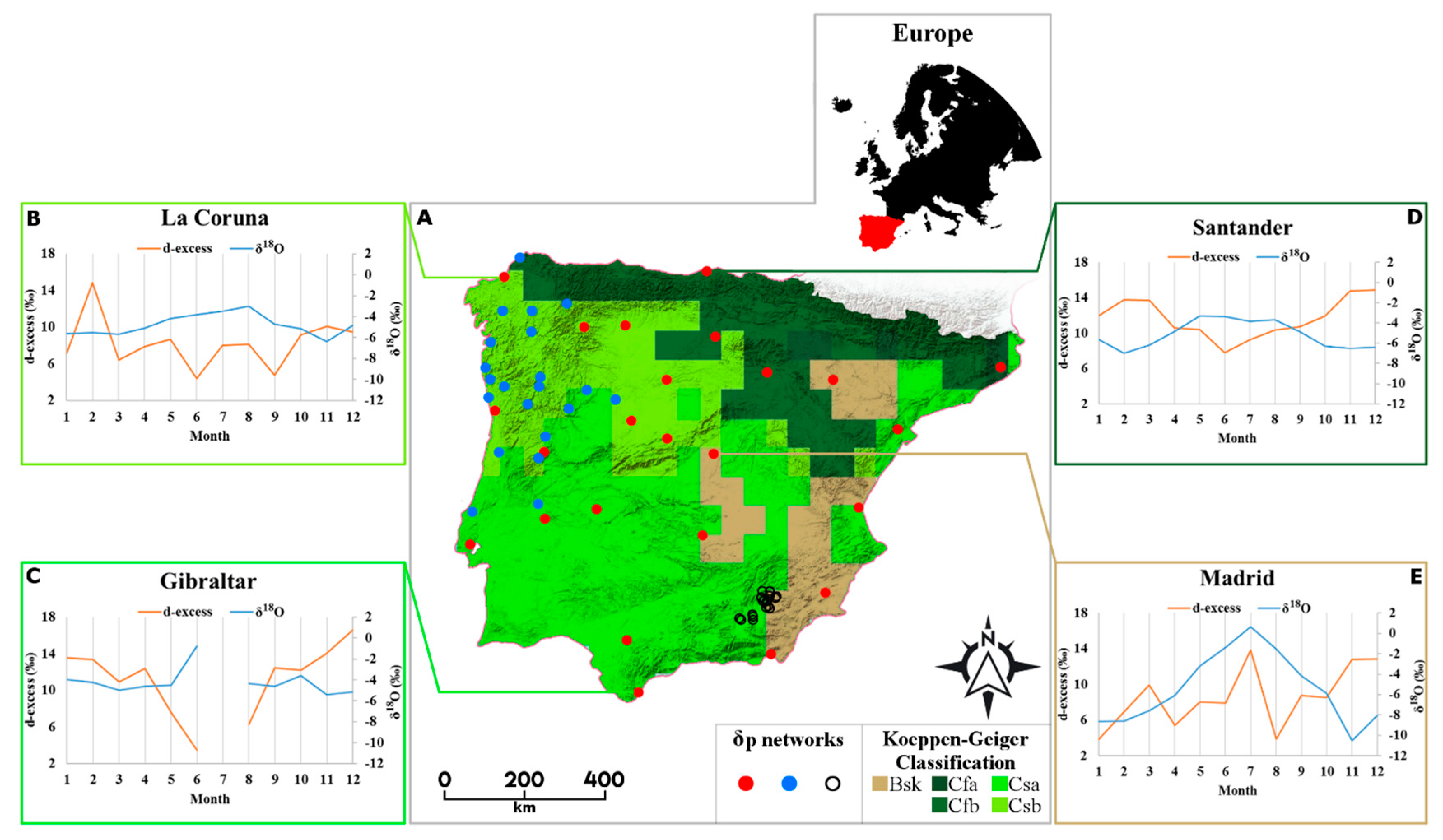
The Iberian Peninsula is located in the mid-latitudes of the Northern Hemisphere between the Mediterranean Sea and the Atlantic Ocean. Four major climate zones may be delineated on the peninsula (Figure 1A). The greater part might be categorized as warm temperate, with dry, hot, or cool summers (Köppen codes: Csa/Csb, respectively; Figure 1A), where dry hot summers are dominant (Csa;), and the value of δp had risen to around zero during the light summer rains (Gibraltar, Figure 1C). The values of d-excess (d = δ2H – 8 × δ18O, [1]) indicate an intra-annual trend with the minimum being reached in mid-summer.
Cool summers are more frequent (Csb) in the northwestern parts of the peninsula. The proximity of the ocean causes both milder winters and cooler summers, as well as provides an abundant moisture supply, giving a fair amount of annual precipitation evenly distributed over the year [32]. Precipitation δ18O values are usually below −3‰, peaking in August with a dampened intra-annual trend characteristic of d-excess as well (e.g., La Coruña; Figure 1B). This was generally below 10‰.
Cold, semi-arid (BSk) conditions are prevalent in the more elevated central and southeastern regions of the peninsula. These result in the most characteristic intra-annual pattern in terms of stable isotopic features of precipitation. In Madrid, for instance, the seasonal amplitude of δ18Op is ~12‰ and the maximum δ18Op occurs in mid-summer (July) (Figure 1E). A similar δ18Op pattern was reported for the years 2000–2002 [24]. Monthly d-excess values are characteristically below 10‰.
Humid warm summers (Cfb) characterize the northern sector of the peninsula, in the vicinity of the Pyrenees and along the Cantabrian coast. Here, precipitation δ18O shows a minimum value in February and a maximum in May (e.g., Santander, Figure 1D). Deuterium-excess displays a relatively small degree of seasonal fluctuation, with monthly values characteristically above 10‰.
The most important moisture sources for the region are the tropical-subtropical North Atlantic corridor, the western Mediterranean basin, and recycled water from the Iberian land-mass, though to a varying extent intra-annually. In winter, the Atlantic serves as almost the exclusive moisture source in the western parts of the peninsula [26], and no influence from the Mediterranean moisture could be detected west from ~5°W longitude [27]. In summer, the western Mediterranean region provides almost twice as much moisture as North Atlantic, and it has a stronger effect in the eastern regions [26,27].
2.2. Used Materials
Precipitation oxygen and hydrogen stable isotope composition is conventionally expressed in δ values: the ratio between the heavy and light stable isotopes (i.e. 18O/16O or 2H/1H) in the sample when compared to the Vienna Standard Mean Ocean Water (V-SMOW), being expressed in per mill [33].
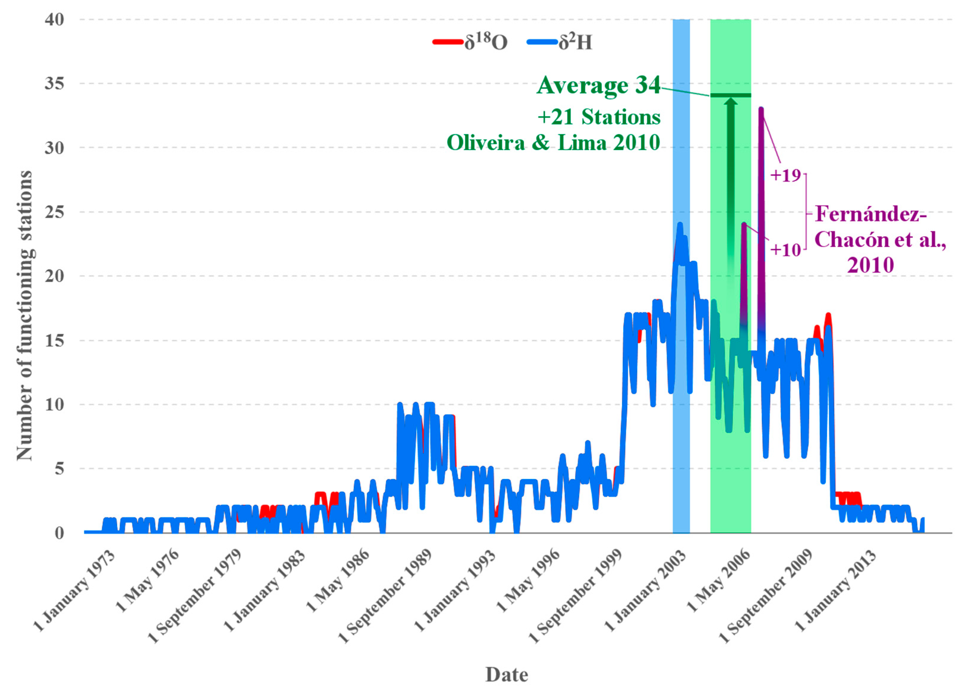
Monthly δp values were acquired from 32 Iberian stations of the Global Network of Isotopes in Precipitation (GNIP). The available data were unequally distributed in time and space (Figure 1 and Figure 2). Historically, after Gibraltar, the second station was Faro, while the GNIP network on the peninsula became spatially extensive after May 1988, with 10 stations. Between 1992 and 1998, the number of simultaneously operating stations once again fell to ~5. The number of operating stations was usually ≥15 between 1998 and 2011, after which once more, only two stations, Gibraltar and Riells, were gathering samples [23]. The point at which the network was at its most extensive was in January 2003, when 24 monitoring sites were operating simultaneously (Figure 2). In the period assessed here (October 2002–September 2003), the same number of data were generally available for both water stable isotopes, although, in certain cases, the δ18O records were more abundant (red line in Figure 2).
The opportunity arose to expand the GNIP dataset with precipitation stable isotope data from two regional monitoring campaigns (Figure 1A and Figure 2). In the first case, 21 stations were available in NW Iberia (October 2004–June 2006) [35]. In the second case, 10 stations (May 2006) and 19 stations (April 2007) were available from SE Iberia [36]. The SE regional network is located in a spatially more confined mountainous area with abrupt differences in elevation between neighboring sites, while that in the NW is better distributed, both vertically and horizontally over a larger region. Unfortunately, merging the GNIP and SE Iberia datasets drew attention to a critical lack of spatial homogeneity (Figures S2–S4), and this turned out to be unsuitable for use in the geostatistical analysis (for details, see Electronic Supplementary Materials), unlike the combination of the GNIP and the NW network. In the latter case, the average number of stations with available records from the GNIP database (~13) increased to ~34 for the period October 2004 to June 2006 (Figure 1 and Figure 2).
The precipitation records archived alongside monthly δp values in the GNIP database were found in some cases to have gaps and/or be erroneous, raising questions regarding the calculation of seasonal and annual precipitation-amount weighted averages from monthly δp values. Therefore, gridded (0.5° 0.5°) monthly rainfall totals from the Global Precipitation Climatology Centre (GPCC) database [38], derived as precipitation anomalies at stations interpolated and then superimposed on the GPCC Climatology V2011 [39], were utilized instead. Nevertheless, there were some discrepancies between the monthly precipitation in the GNIP records and the corresponding GPCC values: rmin = 0.82 (Gibraltar), rmax = 0.99 (Almeria Aeropuerto), and rmean = 0.95 (17 GNIP stations) for 2000–2013. An obvious advantage of the gridded data set is the lack of gaps and the fact that it is less prone to single-station error.
2.3. Methodology
2.3.1. Steps of the Analysis and Preprocessing
The first step in data preprocessing was to numerically check the δp values for database errors (e.g., typos, sign errors) [40]. For example, very negative d-excess values, occasionally even lower than −10‰, corresponding to a monthly precipitation total exceeding 5 mm was all carefully compared to the surrounding stations. The negative d-excess value was interpreted as evidence of evaporative enrichment of the sample and it was discarded from the evaluation if no neighboring stations reported similarly extreme d-excess value for the given month. In addition, in July 2003 at GNIP station Madrid, somewhat improbably, the same values were found as in June, without any precipitation in July being recorded at that site. Consequently, the fact that the June values reappeared in July was suspected to be a database error, and was thus omitted.
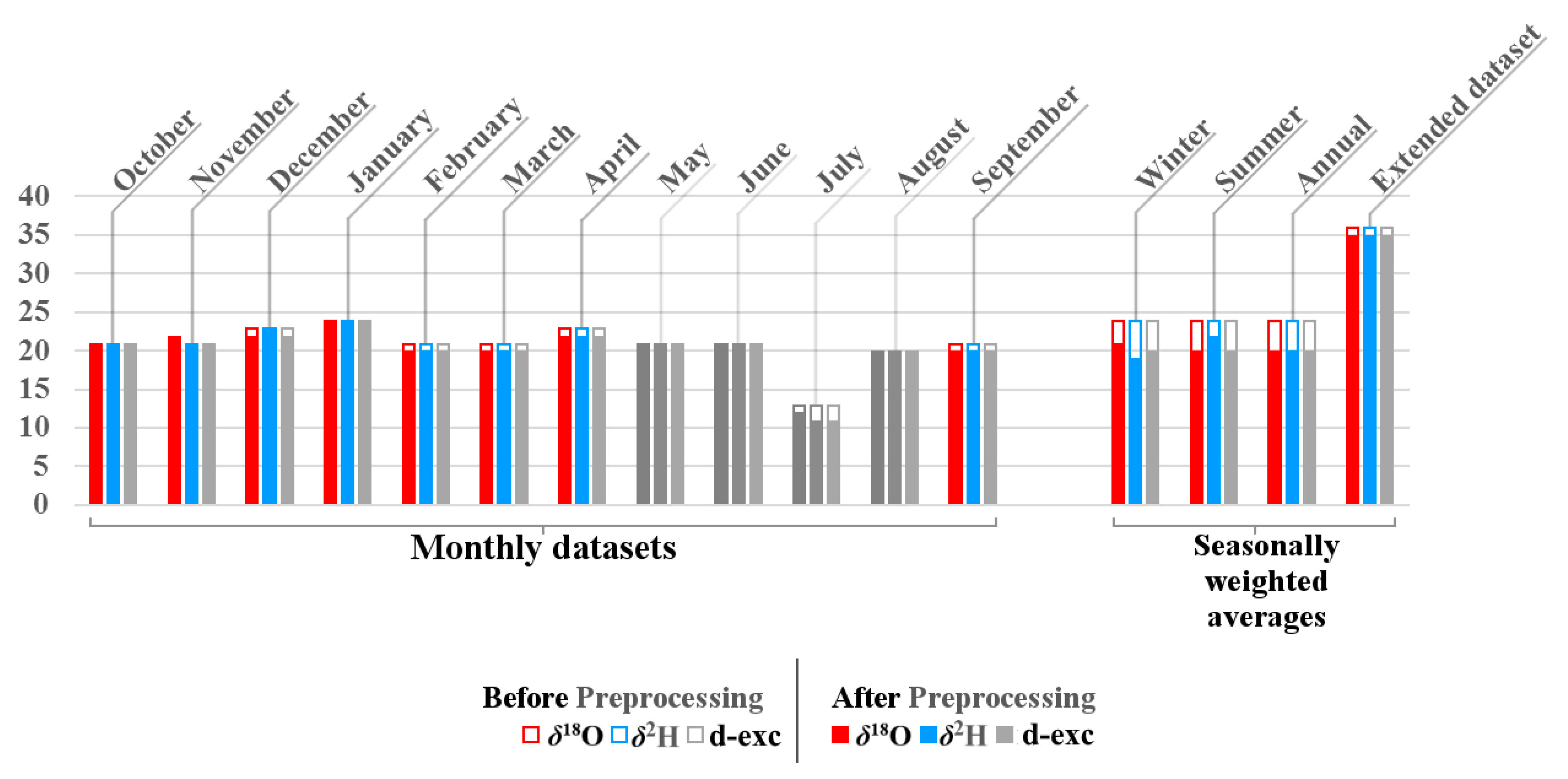
Due to the low amount, or frequently the complete lack of precipitation in summer in southern and eastern Iberia (Figure 1), the May to August monthly data were discarded from the analysis (grey bars in Figure 3). Nevertheless, the summer (defined as April to September) seasonal average was calculated, despite the unrealistically low values of d-excess and high values of δp, because the corresponding precipitation amounts were also low, having only a small impact on the amount weighted summer seasonal value.
An amount-weighted mean was only calculated for a period (season, year) if at least 75% of the fallen precipitation was analyzed for the given isotope. This required completeness is a bit stricter criterion than the GNIP protocol (70%) [40].
2.3.2. Multiple Regression Analysis
Trend-like tendencies in δp over large distances across the Iberian Peninsula have been documented [24,29,35]. These empirical relationships of δp with geographical factors (e.g., altitude effect) may mask the finer scale spatial autocorrelation patterns, which are the focus of interest in the present investigation. The effect of the geographical factors influencing the water stable isotopes’ variability in precipitation first has to be minimized in order to obtain representative results with variography (Section 2.3.3), i.e. the spatial trend has to be removed from the data to obtain second-order stationarity [41]. Thus, the effect that was linked to the geographical factors was minimized by computing best-fit multiple regression models and determining their residuals.
The investigation was conducted while using the stepwise procedure suggested by O’Brien, with latitude, longitude (Web Mercator EPSG: 3857), elevation, and geodetic distance from the coast as the independent predictor variables, and the primary precipitation stable isotope values as the dependent variables [42]. Of the four independent variables, the first three were found to be applicable to the minimalization of the effect of geographical factors influencing the raw δp records. Probabilities ranged between p < and p < 0.04, variance inflation was negligible (Variance Inflation Factor < 1.187), and the average adjusted values of R2 were 0.63 and 0.58 for δ18Op and δ2Hp, respectively (Table S1). No trend removal was found to be necessary in the case of the derived isotopic parameter (d-excess). A similar multiple regression approach was applied to determine the degree of dependence of δp on the geographical variables in Central America [43]. However, the advantage of the present approach is that it uses Variance Inflation Factor to control possible multicollinearity [42].
Moran’s I global statistic [44] was calculated (binary weighting, bandwidth = 4) for all three isotopic parameters, to investigate whether the residuals carry significant spatial information vital for the derivation of the desired isoscapes.
2.3.3. Variography
The basic function of geostatistics, the variogram, was used to explore the spatial autocorrelation structure of δp and d-excess in the Iberian Peninsula. The empirical semivariogram might be calculated while using the Matheron algorithm [45], where is the semivariogram and and are the values of a parameter sampled at a planar distance from each other
N(h) is the number of lag-h differences. The most important properties of the semivariogram are the nugget, quantifying the variance at the sampling location (including information regarding the error of the sampling), the sill (c), that is, the level at which the variogram stabilizes, and the range (a), which is the distance within which the samples have an influence on each other and beyond which they are uncorrelated [46]. Note here, that reported ranges in the study are planar distances (dplanar) in km (EPSG: 3857), unless otherwise reported; estimated average conversion in the region: dplanar × 0.755 = dgeodetic. In practice, an obtained range is usually attributed to environmental processes that act on the same scale as the range of the specific variable [46], and they are known to have a physical relationship with the assessed variable. In addition, a nugget-type variogram is obtained if the semivariogram does not have a rising part and the points of the empirical semivariogram align parallel to the abscissa. In this case, the sampling frequency is insufficient for estimating the sampling range while using variography [13].
The semivariograms that were derived from the monthly GNIP data required 10 bins and a maximum lag distance of 540 km to achieve the most uniform number of station pairs in the analysis, while, in the case of those from the extended dataset, these figures were 20 bins and a maximum lag distance of 660 km. For geostatistical modeling (e.g., kriging), theoretical semivariograms have to be used to approximate the empirical ones [47]. In practice, the spherical and Gaussian models are among the most commonly used theoretical semivariograms. These were, in fact, applied in the present study by least squares model fitting [48]. While a spherical model displays a linear behavior at the origin and the sill is reached at a, a Gaussian has a repressed slope (tangent with zero slope at the origin), and its sill is a limited value that might be approximated to an infinitesimal degree, but never reached. Thus, in the case of the Gaussian model, a practical and an effective range ae = a × √3 have to be determined; ae is then used for further geostatistical modeling [46,49].
As the final step in the data preprocessing, semivariogram clouds were utilized to search for additional outlying values. These then had to be omitted following a detailed investigation, resulting in the final set and number of data as the input for the variography (Figure 2). The amount weighted seasonal averages were only calculated after this step has been taken; hence, monthly values that were omitted on the basis of the semivariogram clouds were also treated as missing isotopic parameters.
2.3.4. Isoscape Derivation with Kriging
The isoscape was derived with a three step residual kriging procedure [12,13,31,50]. As a first step, an initial grid (10 × 10 km) of stable isotope variation was derived in the region described by the multiple regression model of the supposedly driving geographic variables (LAT, LON, ELE; for details, see Sect. 2.3.2). Next, an interpolated (ordinary point kriging) residual grid was modelled while using the theoretical semivariogram (Section 2.3.3) that was fitted on to the residuals of the multivariate regression model. Note here that a methodological comparison testing various interpolation methods for the residual field of δp in the central and eastern Mediterranean region reported that the best results were obtained while using ordinary kriging to derive the residual grid [50]. Finally, the initial and residual grids were summarized to obtain the final isoscape.
All of the computations were performed while using Golden Software Surfer 15, GS+ 10, and the raster [51] and lctools [52] packages in R [53]. The digital elevation model was retrieved from Shuttle Radar Topography Mission data [54] while using Global Mapper. Gimp 2.8 and MS Excel 365 were used for certain visualizations of the results.
3. Results and Discussion
The obtained significant (p < 0.05) global Moran’ Is for each isotopic parameter range between 0.18 and 0.27, indicating positive spatial autocorrelation in the residuals. This encouraged the incorporation of the ‘residual spatial patterns’ in the derivation of the isoscapes with variography.
3.1. Variography Using GNIP Data
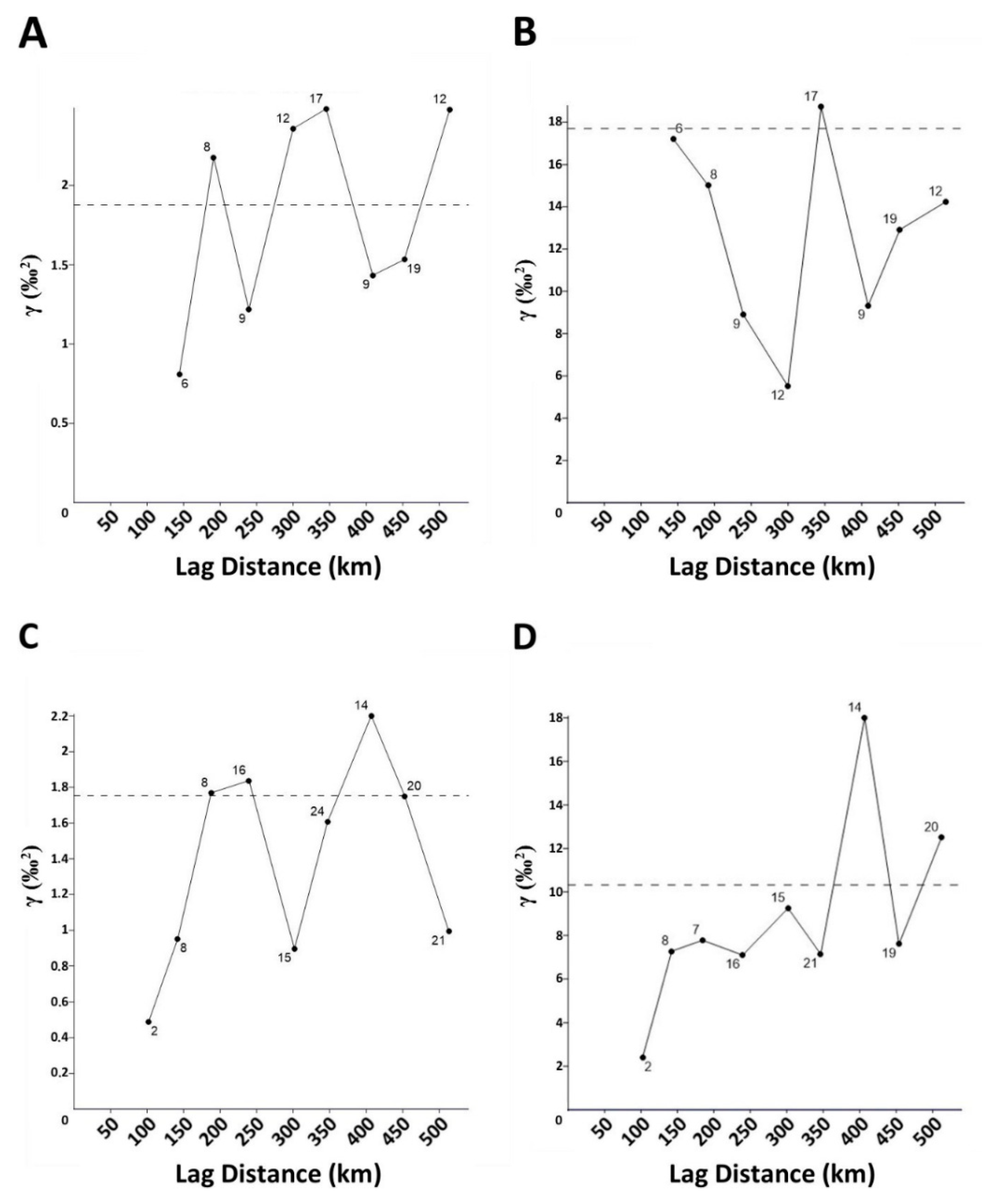
Variogram analysis was first conducted on monthly residuals of the δp records of GNIP stations, and then the amount weighted seasonal averages (winter: October–March; summer: April–September) and the annual residuals (Table S2). With regard to δ18Op, three of 12 the semivariograms (two monthly, January, March see Figure 4A, and one seasonal, summer) were of the nugget-type, while, in the case of δ2Hp, this was true for two of the 12 cases (two monthly: January, March). Turning to d-excess, eight out of 12 semivariograms (five monthly: October, November, January, February, March see Figure 4B, 2 seasonal: summer, winter, and the annual) were of the nugget-type.
Unfortunately, a fair portion of the theoretical semivariograms proved to be unsatisfactory due to the lack of data from short distances. There is no month for which it can be said that there are both (i) stations sampling within a 50 km of each other and (ii) more than two stations sampling simultaneously in a 100 km distance. Worse still, in e.g., March 2003, there was no station pair sampling within a 100 km radius (Figure 4A,B), a critically low degree of coverage. Therefore, the small variances over short distances were not observed, only large variance over long distances. Unfortunately, the fitting of theoretical semivariograms was not performed because of the low number and the lack of station pairs at the shortest distances, even in those cases where the semivariogram did outline a rising section (Figure 4C,D). Besides the spatial deficiency of the GNIP network discussed above, the partial evaporation of raindrops [55] during the events with only a few millimeters of precipitation—typical in hot Mediterranean summers—can also result in local noise, further encumbering the geostatistical analysis of the δp signal. The fact that unusual δp characteristics were reported for S Europe [56,57] during the severe European heat waves of 2003 [58] seems to concur with this statement.
3.2. Variography Using the Extended Database
There was a unique opportunity to extend the δp records of the GNIP stations with an additional dataset [35] covering a two year period (October 2004–June 2006; Figure 1 and Figure 2). The station network of this regional ad hoc sampling campaign provided a seamless union with the coexisting GNIP data set (Figure S1). The merged dataset had a greater amount of short distance data pairs than that from the GNIP stations. The Gaussian semivariograms that were fitted to the empirical variograms of δ18Op (Figure 5A) and δ2Hp (Figure S5) obtained from the merged GNIP & NW dataset indicated a ~510 km and a ~420 km range, respectively. For the d-excess, a spherical semivariogram indicated a range of ~440 km (Figure 5B). If these ranges are considered to define the isotropic impact areas, the extended network provides full spatial coverage of the peninsula regarding all three parameters (Figure 5 and Figure S5).
In the meanwhile, a shorter spatial range (below ~100 km) seems to be present in the case of the primary isotopic variables, however this remains speculative and needs further investigation.
The determined spatial range (average ~450 km in planar distance) indicated by the primary isotopic parameters and the range of d-excess refer to a substantial change in the spatial correlation structure of isotopes in precipitation at the scale of the zonal extension of the peninsula. The spatiotemporal variability of moisture contribution over the Iberian Peninsula can link this observation. Studies agree that the Atlantic Ocean and the Mediterranean Sea are the primary marine moisture sources, with a varying degree of spatial- and intra-annual dominance over the peninsula [26,59]. In addition, a characteristically different isotope-hydrological signature is observed between the Mediterranean (d-excess ~16‰) and the Atlantic (d-excess ~10‰) moisture sources (e.g., [28,60]). The recently documented division at ~5°W longitude separating the western part of the peninsula with no influence from the Mediterranean moisture in winter, from the eastern part where western Mediterranean moisture is prevailing during spring and summer seasons [27], is well in line with the above interpretation.
3.3. Isoscape of Precipitation Oxygen and Hydrogen Stable Isotopes for the Iberian Peninsula
The initial grid of δ18Op derived from the multiple regression model of the “Extended dataset” (Table S1) was combined with the residual grid that was obtained with the Gaussian semivariogram while using Equation (2) to derive the estimated values of δ18Op (Figure 6A)
where A and B stand for zonal and meridional Web-Mercator coordinates (EPSG: 3857), respectively, C for elevation and D for the residual grid. With a similar procedure, the δ2Hp isoscape was also derived (Table S1, Figure S6).
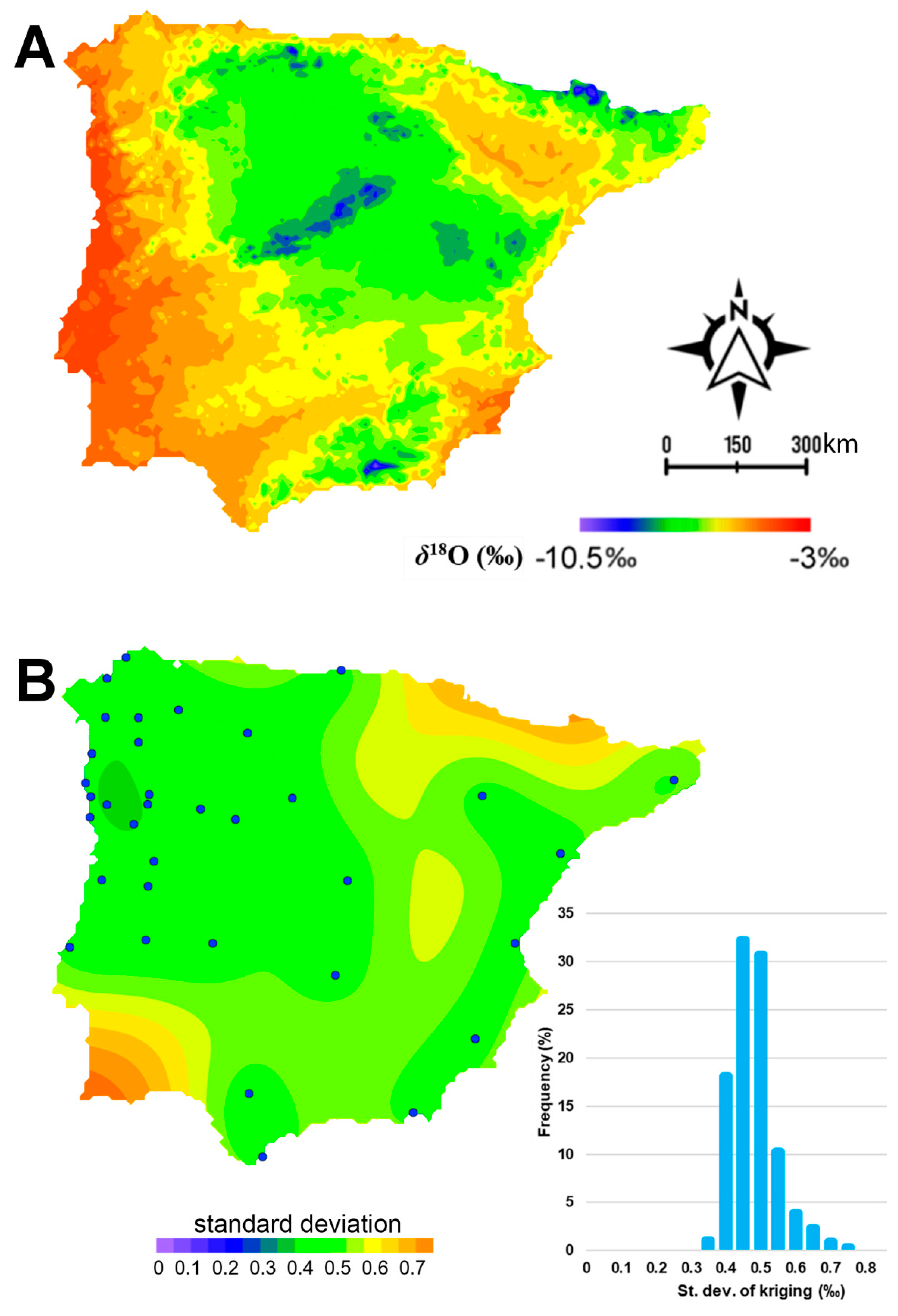
The δ18Op values that were indicated by the obtained isoscape range between −10.55 and −3.97‰ (Figure 6A). The estimations error is < 0.5‰ at the stations, while the largest error (~0.75‰) is obtained in areas where station data were not available (as usually observed, see [14]) e.g., in the northern (Pyrenees) and SW part of the peninsula (Algarve) (Figure 6B). A similar pattern is seen for δ2Hp with values ranging from −76.6 to −21.1‰ (Figure S6A) and estimated errors up to 6‰ (Figure S6B).
The presented δp isoscapes for the Iberian Peninsula can be compared to former products (models and maps) predicting/featuring the spatial distribution of amount-weighted long-term precipitation water stable isotopes across the Iberian Peninsula. A map of δ18Op distribution in peninsular Spain and the Balearic Islands was produced using composite monthly samples for the period 2000–2006 of 15 GNIP stations, belonging to the Spanish network for isotopes in precipitation (REVIP) in a polynomial model while employing latitude and elevation as predictors [29]. The REVIP-based map is not available in numerical format, so only the mapped features and some methodological differences can be evaluated. The most striking similarity is that both the current δ18Op isoscape (Figure 6A) and the REVIP-based map [29] capture the orography-induced isotopic depletion for high reliefs. The polynomial model with geographical factors can be regarded as an analogue of the initial grid of this study. Thus, the added value of the presented isoscape is the consideration of the spatial variability that is retained in the model residuals irrefutably carrying sub-regional information. For example, zonal heterogeneity of vapor sources [13,14,31], which is especially interesting information from an isotope-hydrometeorological perspective and must be taken into account to improve regional isotopic landscapes. Indeed, ignoring the δ18Op residual variance might inspire the debatable conclusion that Atlantic Ocean is the main source of water vapor over the region [29], since the isotope-hydrometeorological dichotomy reflecting the dual moisture sources, clearly also expressed by recent atmospheric transport models [26,27], could be captured in the residual field. Finally, technical advancements in the current δ18Op isoscape when compared to the REVIP-based map are that the extended station network (14 more stations from Portugal, 6 from Spain and another one from Gibraltar) definitely (i) improved the accuracy of both the fitting of the regression model and the subsequent interpolation and (ii) extended the coverage of the mapping to the entirety of the peninsula.
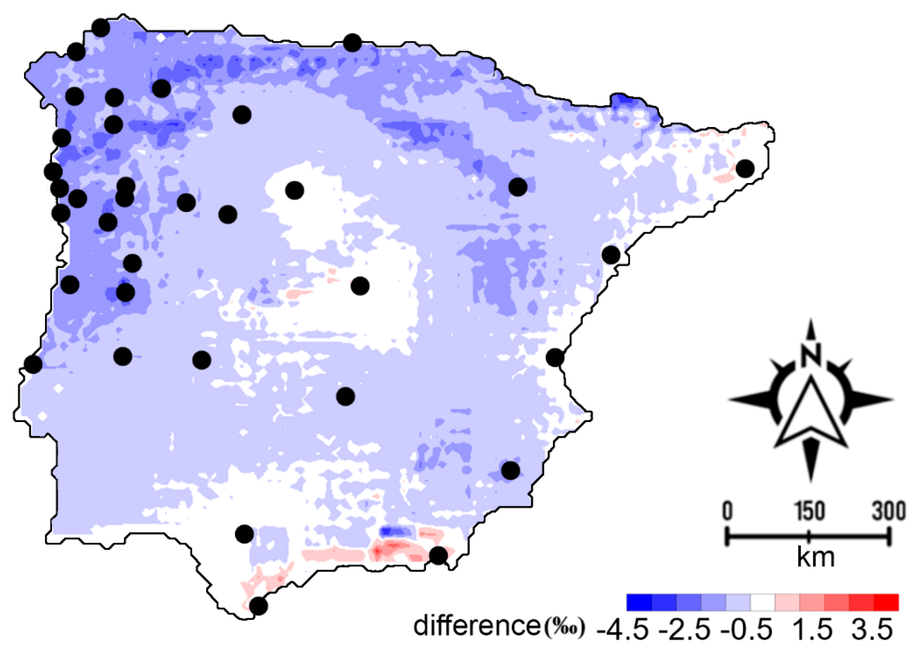
Data products and estimated spatial errors of the global regionalized cluster-based water isotope prediction (RCWIP) model [16] are both freely available [61], so detailed numerical comparison between the Iberian subset of RCWIP model and the current regionally fitted δp isoscapes could be calculated by subtracting the present model values from the resampled (10 10 km) RCWIP ones. Their difference maps (Figure 7 and Figure S7) indicate more positive values that were obtained by the current model over the mountains: such as the Pyrenees, the Cantabrian Massifs, in a small patch covering the peak region of the Beatic Cordilleras, and along the Iberian System. Major regional patterns in the difference maps are (i) lower values in the RCWIP over extended part of the Atlantic and Cantabrian regions (difference < −2.5‰ for δ18Op and < −5‰ for δ2Hp), while (ii) positive differences along the southernmost part of the peninsula (difference > 1.5‰ for δ18Op and > 10‰ for δ2Hp) indicate that RCWIP model predicted higher values south from the Beatic Range (Alboran Coast). Over a remarkably large part of the central (e.g., Meseta, Andalusia) and northeastern part (e.g., Ebro Basin, including the coast of the Balearic Sea) of the peninsula the predicted δp values agree (Figure 7 and Figure S7). Two climatic zone domains in the RCWIP model cover the Iberian Peninsula [16], however their boundary does not separate the positive and negative field seen in the difference maps (Figure 7 and Figure S7). Moreover, the predicted values agree very well for extended areas within both RCWIP zones, so the regional scale differences likely do not reflect the RCWIP zones. The differences cannot be explained by the incorporation of the additional samples from the northwestern sector of the peninsula [35], either, because (i) the region of negative difference also extends to the Cantabrian Coast, from where no station was included in the complementary dataset and (ii) the field of positive anomalies along the Alboran Coast is situated >500 km form the area covered by the complementary dataset. It is suggested that the regional patterns seen in the difference map are evidence of a considerable improvement in the current regional prediction of the spatial distribution of long-term mean δp across the Iberian Peninsula.
The kriging error of the presented Iberian precipitation isoscape (as seen from the in-set histograms; Figure 6B and Figure S6B) is smaller by more than a factor of two for the Iberian Peninsula when compared to the RCWIP model [16], where it ranged between 0.96–0.98‰ for δ18Op and 7.9–8.1‰ for δ2Hp. Thus, the presented isoscape provides a more precise estimation of δp than the regional subset of the RCWIP model. This is in harmony with the statement, where the derivation of regional isoscapes is suggested to better estimate the regional variability of δp [16], since these do take local geographical features or meteorological parameters into account, which could influence local rainfall patterns leading to a good agreement between observed and modelled data, unlike global isoscapes [11].
It should be noted that these differences in mean predictions might partly reflect different temporal coverage. The RCWIP is a long-term climatological average that is based on pooled non-continuous decadal-scale data for 1960–2009 for δp, while the Iberian isoscape covers a narrower interval (2004–2006). Moreover, the differences in prediction uncertainty are almost certainly affected by different time-averaging i.e. the uncertainty in RCWIP model parameters includes uncertainty that is associated with predicting average values at stations that sample different periods of time, while, in the case of the present Iberian isoscape, this was not the case.
4. Conclusions
The monthly GNIP δp records (October 2002–September 2003) for 32 stations distributed across the Iberian Peninsula appear to be unsatisfactory for use in the determination of a sampling range of isotope hydrometeorological parameters with variography. However, extended by the addition of a 21-station regional dataset (for the period October 2004–June 2006), a much denser spatial coverage was obtained, proving to be suitable for the exploration of the spatial autocorrelation structure of δp across the Iberian Peninsula. Gaussian semivariograms were modelled for δ2Hp and δ18Op, and an additional one for d-excess with ranges corresponding to ~450 km in planar distance (~340 km in geodetic distance). The ~450 km spatial range is thought to be related to hydroclimatological processes prevailing on the scale of the zonal extension of the peninsula and they could be connected to a spatiotemporal switch between Atlantic and Mediterranean moisture sources. A sparser network (e.g., GNIP) might also prove to be representative since the obtained spatial range of the δp monitoring network provides a coverage for the peninsula. It means that the GNIP monitoring network is suitable for exploration of large-scale isotope hydrological processes/phenomena in the peninsula, but its verification could only be done with a denser network. Finally, the results encourage the development of precipitation stable isotope models at a sub-continental scale in further regions.
Supplementary Materials
The following are available online at https://www.mdpi.com/2073-4441/12/2/481/s1, SuppText.pdf: Additional methodological description (including Figures S1 to S6, and Table S1), Table S2: Stable isotopic data used in the study. Additionally, predicted amount-weighted isoscapes (Figure 6A and Figure S6A) are provided in GEOtiff format.
Author Contributions
Conceived and designed the study: Z.K., I.G.H. Performed the analysis and produced the figures: I.G.H., D.E. Analyzed the data: Z.K., E.D., I.G.H. Wrote the paper: Z.K., P.V., I.G.H., E.D. We applied the FLAE approach for the sequence of authors; see 10.1371/journal.pbio.0050018. All authors have read and agreed to the published version of the manuscript.
Funding
This research was funded by the National Research, Development and Innovation Office; under Grant SNN118205; Slovenian Research Agency ARRS under Grant: P1-0143 and N1-0054; the MTA under Grant “Lendület” program (LP2012-27/2012), and the Ministry of Human Capacities under Grant NTP-NFTÖ-17-B-0028.
Acknowledgments
The authors would like to thank Paul Thatcher for his work on our English version. This is contribution No. 67 of 2ka Palæoclimatology Research Group. This paper is dedicated to the memory of Antal Füst (1940-2020), a pioneer of Geomathematics.
Conflicts of Interest
The authors declare no conflict of interest.
References
- Dansgaard, W. Stable isotopes in precipitation. Tellus 1964, 16, 436–468. [Google Scholar] [CrossRef]
- Fórizs, I. Isotopes As Natural Tracers In The Watercycle: Examples From The Carpathian Basin. Studia UBB Phys. 2003, 1, 69–77. [Google Scholar]
- Bowen, G.J.; Good, S.P. Incorporating water isoscapes in hydrological and water resource investigations. Wiley Interdiscip. Rev. Water 2015, 2, 107–119. [Google Scholar] [CrossRef]
- Araguas-Araguas, L.; Danesi, P.; Froehlich, K.; Rozanski, K. Global monitoring of the isotopic composition of precipitation. J. Radioanal. Nucl. Chem. 1996, 205, 189–200. [Google Scholar] [CrossRef]
- Rozanski, K.; Araguás-Araguás, L.; Gonfiantini, R. Isotopic patterns in modern global precipitation. In Climate Change in Continental Isotopic Records; Swart, P.K., Lohmann, K.C., McKenzie, J., Savin, S., Eds.; American Geophysical Union: Washington, DC, USA, 1993; pp. 1–36. [Google Scholar]
- Yoshimura, K. Stable Water Isotopes in Climatology, Meteorology, and Hydrology: A Review. J. Meteorol. Soc. Jpn. Ser. II 2015, 93, 513–533. [Google Scholar] [CrossRef] [Green Version]
- Liu, Z.; Bowen, G.J.; Welker, J.M.; Yoshimura, K. Winter precipitation isotope slopes of the contiguous USA and their relationship to the Pacific/North American (PNA) pattern. Clim Dyn 2013, 41, 403–420. [Google Scholar] [CrossRef]
- Gibson, J.J.; Edwards, T.W.D.; Birks, S.J.; St Amour, N.A.; Buhay, W.M.; McEachern, P.; Wolfe, B.B.; Peters, D.L. Progress in isotope tracer hydrology in Canada. Hydrol. Process. 2005, 19, 303–327. [Google Scholar] [CrossRef]
- Kong, Y.; Wang, K.; Li, J.; Pang, Z. Stable Isotopes of Precipitation in China: A Consideration of Moisture Sources. Water 2019, 11, 1239. [Google Scholar] [CrossRef] [Green Version]
- Vachon, R.W.; Welker, J.M.; White, J.W.C.; Vaughn, B.H. Monthly precipitation isoscapes (δ18O) of the United States: Connections with surface temperatures, moisture source conditions, and air mass trajectories. J. Geophys. Res. Atmos. 2010, 115. [Google Scholar] [CrossRef]
- Kaseke, K.F.; Wang, L.; Wanke, H.; Turewicz, V.; Koeniger, P. An Analysis of Precipitation Isotope Distributions across Namibia Using Historical Data. PLoS ONE 2016, 11, e0154598. [Google Scholar] [CrossRef]
- Kern, Z.; Kohán, B.; Leuenberger, M. Precipitation isoscape of high reliefs: Interpolation scheme designed and tested for monthly resolved precipitation oxygen isotope records of an Alpine domain. Atmos. Chem. Phys. 2014, 14, 1897–1907. [Google Scholar] [CrossRef] [Green Version]
- Hatvani, I.G.; Leuenberger, M.; Kohán, B.; Kern, Z. Geostatistical analysis and isoscape of ice core derived water stable isotope records in an Antarctic macro region. Polar Sci. 2017, 13, 23–32. [Google Scholar] [CrossRef]
- Lykoudis, S.P.; Argiriou, A.A. Gridded data set of the stable isotopic composition of precipitation over the eastern and central Mediterranean. J. Geophys. Res. Atmos. 2007, 112. [Google Scholar] [CrossRef] [Green Version]
- Chan, W.-P.; Yuan, H.-W.; Huang, C.-Y.; Wang, C.-H.; Lin, S.-D.; Lo, Y.-C.; Huang, B.-W.; Hatch, K.A.; Shiu, H.-J.; You, C.-F.; et al. Regional Scale High Resolution δ18O Prediction in Precipitation Using MODIS EVI. PLoS ONE 2012, 7, e45496. [Google Scholar] [CrossRef] [PubMed] [Green Version]
- Terzer, S.; Wassenaar, L.I.; Araguás-Araguás, L.J.; Aggarwal, P.K. Global isoscapes for δ18O and δ2H in precipitation: Improved prediction using regionalized climatic regression models. Hydrol. Earth Syst. Sci. 2013, 17, 4713–4728. [Google Scholar] [CrossRef]
- van der Veer, G.; Voerkelius, S.; Lorentz, G.; Heiss, G.; Hoogewerff, J.A. Spatial interpolation of the deuterium and oxygen-18 composition of global precipitation using temperature as ancillary variable. J. Geochem. Explor. 2009, 101, 175–184. [Google Scholar] [CrossRef]
- Clark, I.D.; Fritz, P. Environmental Isotopes in Hydrogeology; Taylor & Francis: Boca Raton, FL, USA; New York, NY, USA, 1997. [Google Scholar]
- Hobson, K.A. Tracing origins and migration of wildlife using stable isotopes: A review. Oecologia 1999, 120, 314–326. [Google Scholar] [CrossRef]
- Heaton, K.; Kelly, S.D.; Hoogewerff, J.; Woolfe, M. Verifying the geographical origin of beef: The application of multi-element isotope and trace element analysis. Food Chem. 2008, 107, 506–515. [Google Scholar] [CrossRef]
- Ehleringer, J.R.; Bowen, G.J.; Chesson, L.A.; West, A.G.; Podlesak, D.W.; Cerling, T.E. Hydrogen and oxygen isotope ratios in human hair are related to geography. Proc. Natl. Acad. Sci. USA 2008, 105, 2788–2793. [Google Scholar] [CrossRef] [Green Version]
- Bowen, G.J. Isoscapes: Spatial Pattern in Isotopic Biogeochemistry. Annu. Rev. Earth Planet. Sci. 2010, 38, 161–187. [Google Scholar] [CrossRef] [Green Version]
- International Atomic Energy Agency (IAEA). Global Network of Isotopes in Precipitation. The GNIP Database. Available online: http://www.Isohis.Iaea.Org (accessed on 12 December 2015).
- Araguas-Araguas, L.J.; Diaz Teijeiro, M.F. Isotope Composition of Precipitation and Water Vapour in the Iberian Peninsula; International Atomic Energy Agency: Vienna, Austri, 2005; pp. 173–190. [Google Scholar]
- Carreira, P.M.M.; Araujo, M.F.; Nunes, D. Isotopic Composition of Rain and Water Vapour Samples from Lisbon Region: Characterization of Monthly and Daily Events; International Atomic Energy Agency: Vienna, Austria, 2005; pp. 141–155. [Google Scholar]
- Gimeno, L.; Nieto, R.; Trigo, R.M.; Vicente-Serrano, S.M.; López-Moreno, J.I. Where Does the Iberian Peninsula Moisture Come From? An Answer Based on a Lagrangian Approach. J. Hydrometeorol. 2010, 11, 421–436. [Google Scholar] [CrossRef] [Green Version]
- Ciric, D.; Nieto, R.; Losada, L.; Drumond, A.; Gimeno, L. The Mediterranean Moisture Contribution to Climatological and Extreme Monthly Continental Precipitation. Water 2018, 10, 519. [Google Scholar] [CrossRef] [Green Version]
- Julian, J.C.-S.; Araguas, L.; Rozanski, K.; Benavente, J.; Cardenal, J.; Hidalgo, M.C.; Garcia-Lopez, S.; Martinez-Garrido, J.C.; Moral, F.; Olias, M. Sources of precipitation over South-Eastern Spain and groundwater recharge. An isotopic study. Tellus B 1992, 44, 226–236. [Google Scholar] [CrossRef] [Green Version]
- Rodriguez-Arévalo, J.; Diaz-Teijeiro, M.F.; Castano, S. Modelling And Mapping Oxygen-18 Isotope Composition Of Precipitation In Spain For Hydrologic And Climatic Applications. In Isotopes in Hydrology, Marine Ecosystems and Climate Change Studies; Internaional Atomic Energy Agency: Vienna, Austria, 2013; Volume 1, pp. 171–177. [Google Scholar]
- Rozanski, K.; Sonntag, C.; Münnich, K.O. Factors controlling stable isotope composition of European precipitation. Tellus 1982, 34, 142–150. [Google Scholar] [CrossRef] [Green Version]
- Bowen, G.J.; Wilkinson, B. Spatial distribution of δ18O in meteoric precipitation. Geology 2002, 30, 315–318. [Google Scholar] [CrossRef]
- Ninyerola, M.; Pons, X.; Roure, J.M. Atlas Climático Digital de la Península Ibérica, Metodología Aplicaciones en Bioclimatología y Geobotánica; Universitat Autónoma de Barcelona, Department de Biologia Animal, Biologia Vegetal i Ecologia (Unitat de Botánica), Department de Geografia: Barcelona, Spain, 2005. [Google Scholar]
- Coplen, T.B. Reporting of stable hydrogen, carbon and oxygen isotopic abundances. Pure Appl. Chem. 1994, 66, 273–276. [Google Scholar] [CrossRef]
- Kottek, M.; Grieser, J.; Beck, C.; Rudolf, B.; Rubel, F. World Map of the Köppen-Geiger climate classification updated. Meteorol. Z. 2006, 15, 259–263. [Google Scholar] [CrossRef]
- Oliveira, A.; Lima, A. Spatial variability in the stable isotopes of modern precipitation in the northwest of Iberia. Isot. Environ. Health Stud. 2010, 46, 13–26. [Google Scholar] [CrossRef]
- Fernández-Chacón, F.; Benavente, J.; Rubio-Campos, J.C.; Kohfahl, C.; Jiménez, J.; Meyer, H.; Hubberten, H.; Pekdeger, A. Isotopic composition (δ18O and δD) of precipitation and groundwater in a semi-arid, mountainous area (Guadiana Menor basin, Southeast Spain). Hydrol. Process. 2010, 24, 1343–1356. [Google Scholar] [CrossRef]
- ESRI. ArcGIS Desktop, 10.5; Environmental Systems Research Institute: Redlands, CA, USA, 2016. [Google Scholar]
- Becker, A.; Finger, P.; Meyer-Christoffer, A.; Rudolf, B.; Schamm, K.; Schneider, U.; Ziese, M. A description of the global land-surface precipitation data products of the Global Precipitation Climatology Centre with sample applications including centennial (trend) analysis from 1901–present. Earth Syst. Sci. Data 2013, 5, 71–99. [Google Scholar] [CrossRef] [Green Version]
- Meyer-Christoffer, A.; Becker, A.; Finger, P.; Rudolf, B.; Schneider, U.; Ziese, M. GPCC Climatology Version 2011 at 0.5: Monthly Land-Surface Precipitation Climatology for Every Month and the Total Year from Rain-Gauges built on GTS-based and Historic Data; Global Precipitation Climatology Centre at Deutscher Wetterdienst: Offenbach, Germany, 2011. [Google Scholar]
- International Atomic Energy Agency (IAEA). Statistical Treatment of Data on Environmental Isotopes in Precipitation; International Atomic Energy Agency: Vienna, Austria, 1992; p. 781. [Google Scholar]
- Hohn, M.E. Geostatistics and Petroleum Geology, 2nd ed.; Springer Science+Business Media: Dordrecht, The Netherlands, 1999. [Google Scholar]
- O’Brien, R.M. A Caution Regarding Rules of Thumb for Variance Inflation Factors. Qual. Quant. 2007, 41, 673–690. [Google Scholar] [CrossRef]
- Lachniet, M.S.; Patterson, W.P. Use of correlation and stepwise regression to evaluate physical controls on the stable isotope values of Panamanian rain and surface waters. J. Hydrol. 2006, 324, 115–140. [Google Scholar] [CrossRef]
- Moran, P.A.P. Notes on Continuous Stochastic Phenomena. Biometrika 1950, 37, 17–23. [Google Scholar] [CrossRef] [PubMed]
- Matheron, G. Les Variables Régionalisées et Leur Estimation: Une Application de la Théorie des Fonctions Aléatoires Aux Sciences de la Nature; Masson et Cie Luisant-Chartres, impr; Durand: Paris, France, 1965. [Google Scholar]
- Chilès, J.-P.; Delfiner, P. Geostatistics; Wiley: New York, NY, USA, 2012. [Google Scholar]
- Cressie, N. The origins of kriging. Math Geol. 1990, 22, 239–252. [Google Scholar] [CrossRef]
- Oliver, M.A.; Webster, R. A tutorial guide to geostatistics: Computing and modelling variograms and kriging. CATENA 2014, 113, 56–69. [Google Scholar] [CrossRef]
- Herzfeld, U.C. Atlas of Antarctica: Topographic Maps from Geostatistical Analysis of Satellite Radar Altimeter Data : With 169 Figures; Springer: Berlin/Heidelberg, Germany, 2004. [Google Scholar]
- Argiriou, A.; Salamalikis, V.; Lykoudis, S. Development and Evaluation of a Methodology for the Generation of Gridded Isotopic Data Sets; Isotopes in Hydrology, Marine Ecosystems and Climate Change Studies, Monaco, 2011; IAEA: Monaco, 2013; pp. 161–169. [Google Scholar]
- Hijmans, R.J. Raster: Geographic Data Analysis and Modeling, 3.0–7. 2019. Available online: https://cran.r-project.org/web/packages/raster/index.html (accessed on 10 December 2019).
- Kalogirou, S. Lctools: Local Correlation, Spatial Inequalities, Geographically Weighted Regression and Other Tools, 3.0-7. 2019. Available online: http://lctools.science/lctools/ (accessed on 10 December 2019).
- R Core Team. R: A Language and Environment for Statistical Computing; R Foundation for Statistical Computing: Vienna, Austria, 2019. [Google Scholar]
- Farr, T.G.; Rosen, P.A.; Caro, E.; Crippen, R.; Duren, R.; Hensley, S.; Kobrick, M.; Paller, M.; Rodriguez, E.; Roth, L.; et al. The shuttle radar topography mission. Rev. Geophys. 2007, 45. [Google Scholar] [CrossRef] [Green Version]
- Stewart, M.K. Stable isotope fractionation due to evaporation and isotopic exchange of falling waterdrops: Applications to atmospheric processes and evaporation of lakes. J. Geophys. Res. 1975, 80, 1133–1146. [Google Scholar] [CrossRef]
- Vreča, P.; Brenčič, M.; Leis, A. Comparison of monthly and daily isotopic composition of precipitation in the coastal area of Slovenia. Isot. Environ. Health Stud. 2007, 43, 307–321. [Google Scholar] [CrossRef]
- Longinelli, A.; Anglesio, E.; Flora, O.; Iacumin, P.; Selmo, E. Isotopic composition of precipitation in Northern Italy: Reverse effect of anomalous climatic events. J. Hydrol. 2006, 329, 471–476. [Google Scholar] [CrossRef]
- Schär, C.; Vidale, P.L.; Lüthi, D.; Frei, C.; Häberli, C.; Liniger, M.A.; Appenzeller, C. The role of increasing temperature variability in European summer heatwaves. Nature 2004, 427, 332. [Google Scholar] [CrossRef]
- Krklec, K.; Domínguez-Villar, D. Quantification of the impact of moisture source regions on the oxygen isotope composition of precipitation over Eagle Cave, central Spain. Geochim. Cosmochim. Acta 2014, 134, 39–54. [Google Scholar] [CrossRef]
- Celle-Jeanton, H.; Travi, Y.; Blavoux, B. Isotopic typology of the precipitation in the Western Mediterranean Region at three different time scales. Geophys. Res. Lett. 2001, 28, 1215–1218. [Google Scholar] [CrossRef]
- International Atomic Energy Agency (IAEA). RCWIP (Regionalized Cluster-Based Water Isotope Prediction) Model—Gridded Precipitation δ18O|δ2H| δ18O and δ2H Isoscape Data, 1st ed.; International Atomic Energy Agency: Vienna, Austria, 2013. [Google Scholar]
Figure 1.
The Iberian Peninsula, with precipitation stable isotope measurement networks and Köppen climate zones [34]. The 24 stations of the Global Network of Isotopes in Precipitation (GNIP) network [23] functioning between October 2002–October 2007 (red solid circles), and two regional networks (NW: [35]; and SE: [36]) are marked with blue solid circles and black circles, respectively (A). The seasonal cycle of δ18Op and d-excess of precipitation of the four characteristic climate zones (B, C, D, E) was computed for mean monthly data of a common six-yr-long (2001–2006) reference period. The color coded Köppen climate zones [34] overlaid on the World_Terrain_Base basemap (Sources: Esri, USGS, NOAA) in ArcMap 10.5 [37]. The red area on the Europe inset map shows the Iberian Peninsula.

Figure 2.
Number of δp records obtained from the GNIP stations and the NW [35] and SE regional networks [36] for the period 1973–2015, during which continuous measurements were performed. The blue vertical rectangle represents the period for which only the GNIP δp records were assessed (October 2002–September 2003; avg. 21 stations). The green rectangle marks the period when the GNIP data was merged with the δp records from the NW network (October 2004–June 2006). The horizontal green line represents the average number of functioning stations [35] in the latter period. The purple lines indicate the number of records of the merged GNIP and SE network [36] for May 2006 and Apr 2007, resulting in 24 and 33 records, respectively.

Figure 3.
The number of precipitation stable isotope records in the initial monthly and multi-monthly datasets before and after preprocessing entered into the semivariogram analysis. Winter: October–March; summer: April–September. Grey bars represent the months omitted from the analysis, see text for details. The open part of a column indicates that some values were discarded after the quality check of the raw data (see Section 2.3.2).

Figure 4.
Empirical semivariograms of δ18Op and d-excess for March 2003 (A, B, respectively) and December 2002 (C, D, respectively). The semivariograms from the March data are of the nugget-type, while the December ones have a rising section. The numbers next to the empirical semivariogram (black dots) show the data pairs within a given distance (bin width was 54 km) behind the semivariograms. The dashed line indicates the average variance.

Figure 5.
Maps representing the sampling sites (left panels: red dots), the range ellipses around them (blue circles) and the empirical (black line with dots in right panels) and fitted theoretical semivariogram (continuous lines in right panels) derived from δ18Op (A) and d-excess (B). For δ18Op (A) the parameters of the Gaussian semivariogram model fitted were C0 = 0.135; C0 + C = 0.635; ae = 507 km; r2 = 0.49; RSS = 0.644. For d-excess (B) the parameters of the spherical semivariogram were C0 = 0.51; C0 + C = 6.105; a = 439 km; r2 = 0.66; RSS = 29.7. The bin width was 33 km; the dashed horizontal line represents the variance. The figure represents the period October 2004–July 2006.

Figure 6.
Predicted amount-weighted δ18Op isoscape for the Iberian Peninsula for October 2004–July 2006 (A) and the standard deviation of kriging (B). Grid resolution: 10 × 10 km. The histogram in panel (B) shows the frequency/abundance of the kriging error in 0.1 bins. The north arrow and scale in panel A is relevant for both maps and the black dots represent the precipitation sampling sites used in the geostatistical analysis representing October 2004–July 2006.

Figure 7.
Difference map of the Iberian subset of the regionalized cluster-based water isotope prediction (RCWIP) model and the one presented in the study. For each grid point the values of the Iberian δ18Op isoscape (Figure 6A) were subtracted from the RCWIP model. Grid resolution: 10 × 10 km, black dots represent the precipitation sampling sites used in the geostatistical analysis representing October 2004–July 2006.

© 2020 by the authors. Licensee MDPI, Basel, Switzerland. This article is an open access article distributed under the terms and conditions of the Creative Commons Attribution (CC BY) license (http://creativecommons.org/licenses/by/4.0/).
Share and Cite
MDPI and ACS Style
Hatvani, I.G.; Erdélyi, D.; Vreča, P.; Kern, Z. Analysis of the Spatial Distribution of Stable Oxygen and Hydrogen Isotopes in Precipitation across the Iberian Peninsula. Water 2020, 12, 481. https://doi.org/10.3390/w12020481
AMA Style
Hatvani IG, Erdélyi D, Vreča P, Kern Z. Analysis of the Spatial Distribution of Stable Oxygen and Hydrogen Isotopes in Precipitation across the Iberian Peninsula. Water. 2020; 12(2):481. https://doi.org/10.3390/w12020481
Chicago/Turabian StyleHatvani, István Gábor, Dániel Erdélyi, Polona Vreča, and Zoltán Kern. 2020. "Analysis of the Spatial Distribution of Stable Oxygen and Hydrogen Isotopes in Precipitation across the Iberian Peninsula" Water 12, no. 2: 481. https://doi.org/10.3390/w12020481
Note that from the first issue of 2016, this journal uses article numbers instead of page numbers. See further details here.