Modeling of Future Extreme Storm Surges at the NW Mediterranean Coast (Spain)

Abstract

Storm surges are one of the main drivers for extreme flooding at the coastal areas. Such events can be characterized with the maximum level in an extreme storm surge event (surge peak), as well as the duration of the event. Surge projections come from a barotropic model for the 1950–2100 period, under a severe climate change scenario (RCP 8.5) at the northeastern Spanish coast. The relationship of extreme storm surges to three large-scale climate patterns was assessed: North Atlantic Oscillation ($NAO$), East Atlantic Pattern ($EAWR$), and Scandinavian Pattern ($SC$). The statistical model was built using two different strategies. In Strategy #1, the joint probability density was characterized by a moving-average series of stationary Archimedean copula, whereas in Strategy #2, the joint probability density was characterized by a non-stationary probit copula. The parameters of the marginal distribution and the copula were defined with generalized additive models. The analysis showed that the mean values of surge peak and event duration were constant and were independent of the proposed climate patterns. However, the values of $NAO$ and $SC$ influenced the threshold and the storminess of extreme events. According to Strategy #1, the variance of the surge peak and event duration increased with a fast shift of negative $SC$ and a positive $NAO$, respectively. Alternatively, Strategy #2 showed that the variance of the surge peak increased with a positive $EAWR$. Both strategies coincided in that the joint dependence of the maximum surge level and the duration of extreme surges ranged from low to medium degree. Its mean value was stationary, and its variability was linked to the geographical location. Finally, Strategy #2 helped determine that this dependence increased with negative $NAO$.

1. Introduction

Human occupation of low-lying coastal regions creates large areas of concentrated human activity, where the population and their property are exposed to coastal flooding. A relevant part of such flooding is due to extreme surges, whose consequences may unleash casualties and infrastructure damage and disrupt essential services [1,2]. Particularly dangerous situations occur when extreme surge levels are combined with ocean waves and a high tide, then resulting in overtopping and breaching of sea defenses [3,4,5]. Low-lying coasts are highly vulnerable areas, in which surges not only drive flooding, but also erosion [6,7]. Extreme surge events are thus an essential driver to be considered in early warning systems and coastal defense planning [8,9,10]. A proper characterization of the extreme surge events can lead to an efficient planning of coastal areas.

The quantification of the effect of climate patterns on extreme surge levels [11,12] is becoming a growing need since large-scale climate patterns represent key modes on the forcings that produce flooding. Although it has been suggested [13] that surge levels would not change in the future or could even slightly decrease [14,15] along the Catalan coast (northwestern Mediterranean Sea), how they will be affected by different climate patterns and the nature of these interactions is still unclear. Among all the climate patterns identified in the Mediterranean Sea [16], the North Atlantic Oscillation ($NAO$; Hurrell and Deser [17]), the East Atlantic West Russian Pattern ($EAWR$; Barnston and Livezey [16]), and the Scandinavian Pattern ($SC$) are some of the most frequently referred to ones for this region [18,19,20,21,22,23].

In a similar way to wave heights [24], surges can be influenced by $NAO$ [25,26]. Significant correlation between $NAO$ and extreme sea levels has already been assessed at the North Atlantic Ocean and Mediterranean Sea [27,28,29,30]. However, not as much is known on the effects of $EAWR$ and $SC$. A relevant question could be how these teleconnection patterns influence both the intensity and duration of storm surges.

The influence of climate dynamics on extremes [12,31,32,33] suggests that extreme surge components should be characterized with non-stationary statistical models, which allow moving trends. Further, a single non-stationary statistical model can include the whole sample of extreme events, whereas stationary models require slicing the sample to address shifting trends. Therefore, non-stationary models perform better than stationary models when characterizing a scarce sample of extreme events.

Additionally, maximum surge levels and surge duration may show correlation [34]. Extreme surge intensity at the Mediterranean can be driven by synoptic conditions that may last for days [35]. Hence, the independence assumption between these variables rarely holds valid. A common method for including dependence among marginal probability distribution functions is with copulas. They have been used extensively in recent works [36,37,38,39]. However, at stationary copulas, the association parameter is kept constant. A plausible hypothesis is that such association parameters may depend on large-scale climate indices. This hypothesis implies that a statistical model for storm surges under changing climates should have non-constant parameters both at the marginals and the copula functions.

This paper aims to characterize storm surge projections at the NW Mediterranean Sea under an RCP 8.5 scenario. Such analysis comprise: (1) fitting non-stationary probability distributions of both the extreme surge levels and their duration at the Catalan coast (northwestern Mediterranean Sea, Figure 1), (2) characterizing the joint probability distribution density of these two variables, under a non-stationary assumption, and (3) establishing the relationship of the frequency of occurrence of extreme surge events, the univariate probability distribution functions, and the joint probability density to $NAO$, $EAWR$, $SC$, and their first two time-derivatives. The fitting sample comes from a barotropic model that spans the whole Mediterranean Sea that uses as forcings sea level pressure and wind fields under an RCP 8.5 scenario. The paper is organized into six sections. Following this Introduction, Section 2 describes the study area. Section 3 describes the theoretical background and the methodology. Section 4 lists the results. Section 5 discusses them, and Section 6 provides the main conclusion.

2. Study Area

The Mediterranean Sea (see Figure 1) is a semi-enclosed basin, delimited by the European, the Asian, and the African continents. It has a narrow connection to the Atlantic Ocean (Gibraltar Strait), as well as access to the Black Sea. This study considers the Catalan coast, which is located in the northwestern Mediterranean sector. The sea bottom of the northwestern Mediterranean, delimited by the coast of the Iberian Peninsula and the longitude $4^{\circ }$E, has a rather mild slope [28]. The continental shelf slope at the southern area is wider than at the northern part. Hence, bottom friction has a more relevant role in the South than at the North.

The Catalan shoreline is oriented in a northeast to southwest manner. Hence, it is heavily exposed to southeastern winds. Eastern winds, which also contribute to extreme surges, are frequent during the summer, triggered by an intense high-pressure area on the British Islands [1]. Along this coast, the level of intense surges (here given by the mean of the three highest annual independent events) is slightly above 20 cm, which is much smaller than the highest values in the Mediterranean Sea (in the north Adriatic Sea, they exceed 60 cm), but is representative of typical values along most of the Mediterranean coastline [14,28].

The $NAO$ teleconnection pattern has a dipole structure, with its negative center over Greenland and a positive center over the Atlantic, whose position shifts seasonally from Europe to North America [16]. The $EAWR$ has its negative center above the northeastern Atlantic and presents a southeastward gradient leading to a positive anomaly band that extends from the Atlantic to the Mediterranean Sea [16]. The $SC$ pattern has a three-lobe structure with a negative center above Scandinavia and positive centers above Western Europe (or just offshore of the Atlantic coast) and Central Asia. $EAWR$ is characterized by a high pressure located over most of Central Europe and bounded by two low pressure centers, over West Russia and the mid-Atlantic. Here, the signs of all anomalies refer to the positive phases and the 500 hPa geopotential maps, where maxima (positive centers) and minima (negative centers) correspond to anticyclonic and cyclonic circulation, respectively [16]. All signs are reversed during the negative phase of these patterns. As an example, it can be seen that the position and speed of the Atlantic jet stream is linked to the phase of $EAWR$ and $NAO$, so that positive $NAO$ corresponds to a northward shift of the jet stream and positive phase of both patterns to its large speed [40].

Both wave climate [19,21,24] and surge levels are affected by climate patterns [27]. Teleconnection patterns have a different effect on waves in the various areas of the Mediterranean Sea, depending also on season [19,23]. Positive $EAWR$ implies lower than average significant wave height (SWH), particularly in the eastern Mediterranean, with a particularly strong effect from January to March. In winter, a positive $NAO$ corresponds to a situation of reduced westerly surface wind and SWH in the northern part of the basin. A positive phase of $EAWR$ implies a large reduction of the northwesterly winds in the western Mediterranean, with a reduction of the SWH of the corresponding wave systems traveling across the basin [23]. Furthermore, a positive velocity of $SC$ leads to an increased total energy of the extreme event [21].

The effect of the wind is not disjoint from that of the teleconnections. $NAO$, $EAWR$, and $SC$ affect the winds and the sea level pressure [23]. The overall interaction of $NAO$, $EAWR$, and $SC$ also has a relevant role on surges, with negative $NAO$ leading to an increase in the number of extreme events and also in their intensity [27].

3. Theoretical Background and Methods

This study consists of a two-step methodology (see Figure 2): (i) a process-based model that provides data on surge; (ii) a statistical model that characterizes the surge extreme events using the data produced by the process-based model. Two strategies for modeling the dependence between the surge components were tested: Strategy #1 (Bivariate Copula Model (BCM)) was related to techniques proposed by [41], and Strategy #2 (non-stationary BCM) was a modified version of Strategy #1, but allowing non-stationarity in the copula parameter. The study was completed with (iii) a validation of the statistical model. The details of the methodology are described in the following sub-sections.

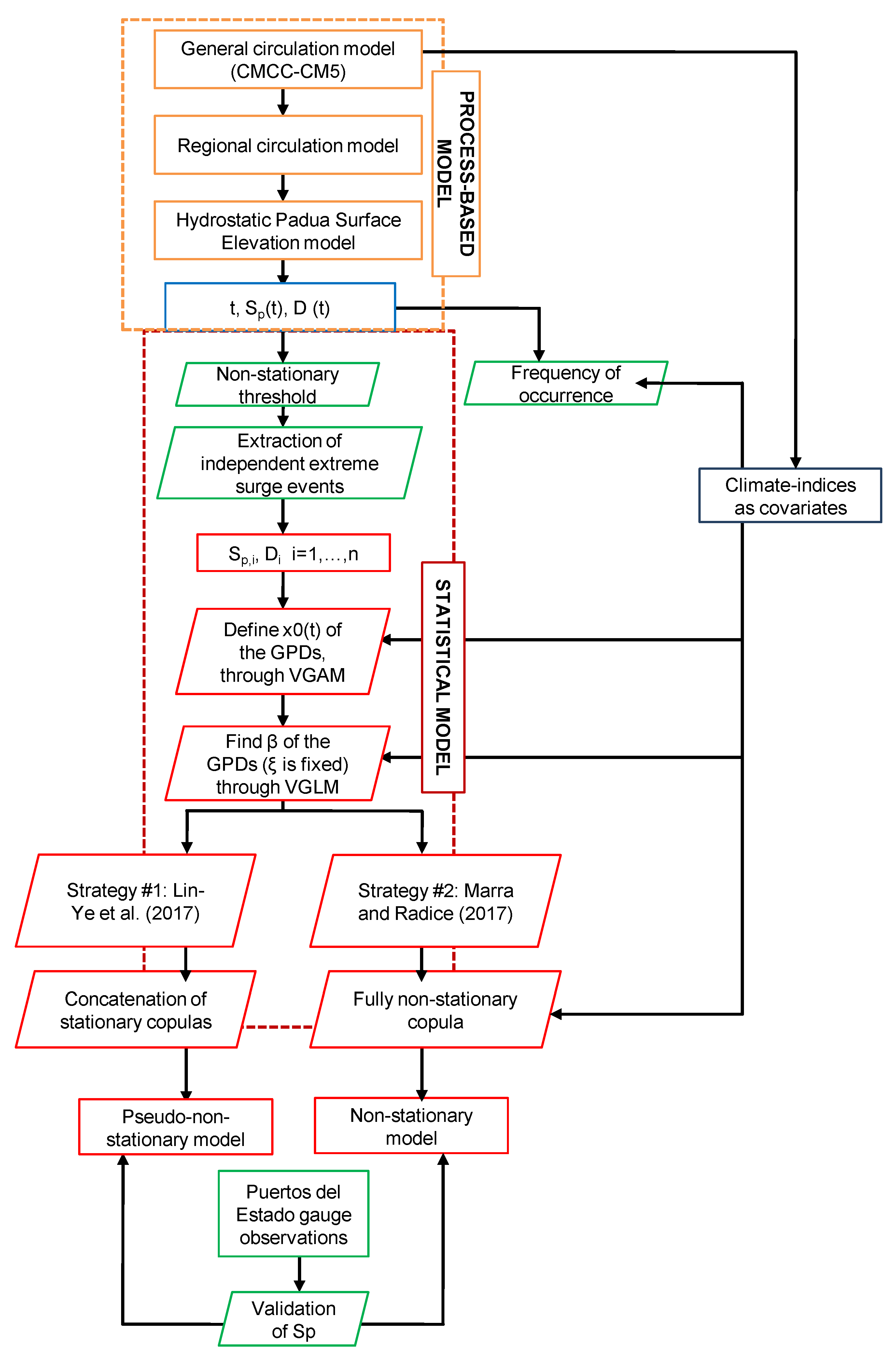
3.1. The Process-Based Model

In the process-based model, dynamical regional projections of storm surge levels (see surge points in Figure 2) were obtained from a deterministic approach, based on the underlying physics. The analysis was performed considering projections of surges at the Catalan coast under a Representative Concentration Pathway 8.5 (RCP8.5) climate change scenario. This scenario considers a CO${}_2$ concentration in the atmosphere close to 1250 ppm in 2100, which is double that of any other scenario in the Fifth Assessment Report [42]. The modeling chain started with the Centro Euro-Mediterraneo sui Cambiamenti Climatici Climate Model (CMCC-CM) [43] Global Circulation Model (GCM). Its latitude and longitude grid sizes were ${0.7484}^{\circ }$ and ${0.75}^{\circ }$, respectively.

$NAO$, $EAWR$, and $SC$ indices were computed from the CMCC-CM GCM monthly-averaged sea level pressure fields. Each climate index was based on the difference of normalized sea level pressure at two specific places. For instance, $NAO$ was estimated from such a difference between Lisbon (Portugal) and Reykjavik (Iceland). They were also scaled to have a mean value equal to zero and a variance equal to unity. In order to avoid sudden events that would hinder interpretation, the time series of climate indices were filtered with a second order low-pass Butterworth filter [44], whose low-pass period was 10 years.

The GCM provides boundary conditions for the Regional Circulation Model (RCM) called COSMO-CLM [45]. The COSMO-CLM grid, which has a resolution of ${0.125}^{\circ }\times {0.125}^{\circ }$, spans the whole Mediterranean region. The next step consisted of applying a 2D horizontal barotropic model, called Hydrostatic Padua Surface Elevation (HYPSE) [46], which was fed with the COSMO-CLM atmospheric pressure and wind fields. The HYPSE and the RCM share the same domain and spatial resolution. The simulation spanned from 1950 to 2100, providing time series for surge with a frequency of 3 h. This process-based model only considered the short-term contribution to sea level variability. Hence, time series were preprocessed using a high-pass filter with a cutoff frequency of 1/30 days, in order to cancel out the long term oscillation of the sea level. For the analysis, these time series, as well as the values of the climate indices were interpolated to the hour.

Two variables were selected to describe an extreme surge event (Figure 3): maximum surge level ($S_p$) and duration of the event (D). D took positive real values; consequently, it was log-transformed for statistical modeling, to avoid scale effects [47] and to be successfully back-transformed to real values.

3.2. Statistical Model

The data obtained from the process-based method could be characterized statistically (Figure 3). Strategy #1 provided a first approximation, with the help of a concatenation of stationary joint probability structures of $S_p$ and D. Then, Strategy #2 was employed, introducing a full non-stationarity of the joint probability structure, estimation of the marginal probability structures of each variable at the same time as the joint probability structure, and the link of the whole joint probability distribution function to the selected climate indices.

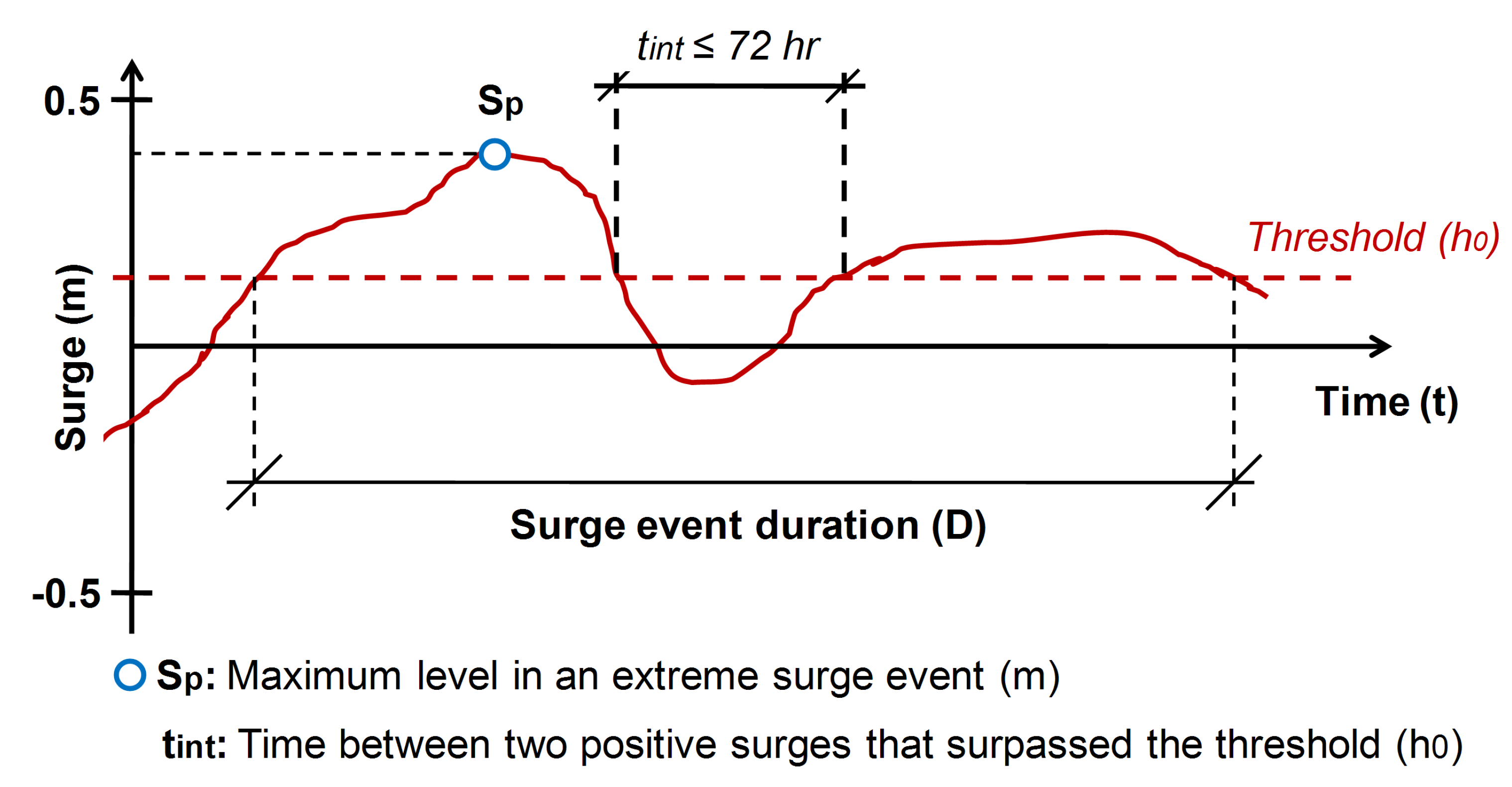
3.2.1. Commonalities of the Two Strategies

In both cases, the non-stationarity of the marginal distribution functions was addressed with a Vectorial Generalized Additive Model (VGAM; Yee and Wild [48]). A VGAM allows a wide range of parametric probability density functions. The parameters related to the storminess, the threshold ($h_0$), and the frequency of extreme events followed a Poisson process ($\lambda$), whereas the surge components were modeled with a Generalized Pareto Distribution (GPD). A VGAM consisted of a linear function [49,50]:

$${\eta }_{i\left(j\right)}={\beta }_{1\left(j\right)}^{\ast }+{\mathrm{f}}_{2\left(\mathrm{j}\right)}\left(x_{i2}\right)+\dots +{\mathrm{f}}_{\mathrm{p}\left(\mathrm{j}\right)}\left(x_{ip}\right),$$

(1)

where ${\eta }_{i\left(j\right)}$ is the $j^{\mathrm{th}}$ dependent variable and $x_i$ is the $i^{\mathrm{th}}$ independent variable that generates ${\eta }_i$. ${\eta }_i$ is the sum of smooth functions of the individual covariates ${\beta }_{1\left(j\right)}^{\ast }$ and $f_{p\left(j\right)}$. Additive models did all the smoothing in $\mathbb{R}$, avoiding the large bias introduced in defining areas in ${\mathbb{R}}^n$. The mathematical assumptions for regression models reflected the degree of confidence of this type of model. These assumptions were: (1) non-correlation, (2) normality, and (3) homoscedasticity of residuals. Assumption 1 was assessed with a autocorrelation function plot. Assumption 2 could be checked with a quantile-quantile plot against an $N\left(0,{\sigma }^2\right)$ distribution, where the sample standard deviation was used as ${\sigma }^2$. Assumption 3 could be analyzed on a scatter plot that contraposed fitted values to residuals.

It was assumed that the relationship between the threshold $h_0$ and any of the following selected factor would follow a Laplace distribution. In order to ensure event independence [34], the minimum time interval between extreme surge events was set to be 72h. A sensibility analysis was carried out on two possible thresholds: 90th and 95th quantiles of the modeled surge series.

The frequency $\lambda$ was a mean value of a counting variable. Therefore, it was a counting variable, as well. In such a case, a Vectorial Generalized Linear Model (VGLM) could be adopted for its estimation [48]. The VGLM was a particular example of VGAM. The relationship of $\lambda$ to a factor such as a climate index could be approximated by a Poisson distribution [51,52].

The definition of a GPD was as follows. $Y=X-x_0$ was the excess of a magnitude X over a location parameter $x_0$, conditioned to $X>x_0$; the support of Y was $\left[0,y_{sup}\right]$ [53]. $y_{sup}$ was the upper bound of the support. The GPD cumulative probability distribution function was, then,

$$F_Y\left(y|\beta ,\xi \right)=1-{\left(1+\frac{\xi }{\beta }y\right)}^{-\frac{1}{\xi }},0\le y\le y_{sup},$$

(2)

where $\beta \ge 0$ is the scale parameter and $\xi \in \mathbb{R}$ is the shape parameter. This $\beta$ should not be mistaken by a covariate of the VGAM.

The non-stationary GPD location parameter $x_0$ was estimated through quantile regression [54]. The quantile regression was a specific type of VGAM, and it estimated the $100\widehat{\tau }\%$ conditional quantile $y_{\widehat{\tau }}\left(x\right)$ of a response variable Y as a function $u\left(x,\tau \right)$ of covariates x. The equation $l_u^{\ast }=l_u+{\varrho }_u{R}_u$ had then to be minimized, where $l_u=\widehat{\tau }{\displaystyle \sum _{i:r_i\ge 0}}\left|r_i\right|\left(1-\widehat{\tau }\right){\displaystyle \sum _{i:r_i<0}}\left|r_i\right|$ for residuals $r_i=y_i-u\left(x_i,\widehat{\tau }\right)$, and $\varrho$ was a roughness coefficient that controlled the trade-off between quality of fit to the data and roughness of the regression function; and R was a roughness penalty [55,56]. Regarding the rest of the GPD parameters: the shape parameter $\xi$ was assumed to remain constant.

The location and scale parameters could be related to the mean and variance of the population through the expressions:

$$\mathrm{E}\left(X\right)=x_0+\frac{\beta }{1-\xi }\approx x_0,\xi <1,$$

(3)

$$\mathrm{Var}\left(\mathrm{X}\right)=\frac{{\beta }^2}{{\left(1-\xi \right)}^2\left(1-2\xi \right)}{\approx \beta }^2,\xi <\frac{1}{2}.$$

(4)

The approximation in Equation (3) remained valid if the orders of magnitude of $x_0$ and $\beta$ were similar.

$NAO$, $EAWR$, $SC$, and their first two time-derivatives were eligible climate indices as covariates for the VGAM [21,52] to predict the threshold $h_0$, the frequency $\lambda$, and the GPD parameters. Using time-derivatives of climate patterns presented an advantage: time-derivatives were associated with variability in the sharp time gradients of these patterns. Up to two climate indices could be used to predict $h_0$, $\lambda$, and $x_0$. If a climate index had clearly much more influence on these parameters, then only this single climate index was used, for the sake of simplicity. A linear interpolation function was selected to relate the covariates to the predictands. The first and second time-derivatives could be written herein as $d\left(·\right)$ and $d^2\left(·\right)$, respectively. For example, the first and the second time-derivatives of $NAO$ could be written as $dNAO$ and $d^{2}NAO$, respectively.

The fitting criteria were to minimize the the Akaike Information Criterion (AIC; Akaike [57]) and the Bayesian Information Criterion (BIC; Tamura et al. [58]). Several combinations of large-scale indices were tested, and those ones with the minimum AIC were chosen. This criterion meant that the selected combination explained more information about the sample than those ones with higher AIC. Additionally, in order to avoid overfitting, the AIC penalized the combination of several large-scale indices (i.e., as the number of covariates grew, the AIC increased). Note that in the figures from Figures 8–13, the discontinuous red line marks the selected large-scale index combination. The degree of influence of the climate indices was quantified in the following manner: Equation (1) can be written as:

$${\eta }_{i\left(j\right)}\approx {\beta }_{1\left(j\right)}+C_r·x_{i2};$$

for $x_{i2}\ne 0$, both sides of the equation could be divided by $x_{i2}$ and be represented as:

$${\eta }_{i\left(j\right)}/x_{i2}\approx {\beta }_{1\left(j\right)}/x_{i2}+C_r,$$

where $C_r$ is the first coefficient of this polynomial expression, and it can be compared to ${\beta }_{1\left(j\right)}/x_{i2}$ (called relative order or $O_{rel}$). In its turn, $O_{rel}$ was herein approximated by the ratio between the mean of the variable and the order of magnitude of the climate index, which was one.

In both strategies, the joint dependence density among several variables could be modeled by a multi-dimensional Archimedean copula. A d-dimensional Archimedean copula has the form:

$$\mathrm{C}\left(\mathbf{F};\varphi \right)={\mathbf{G}}^{-1}\left(\varphi \left(F_1\right)+\cdots +\varphi \left(F_d\right)\right),\mathbf{F}\in {\left[0,1\right]}^d,$$

(5)

for a given generator function $\mathbf{G}$ [59,60,61]. A Gumbel generator could define the dependence in the upper tail of the probability distribution [62]. The fitting criteria was the maximum likelihood method. The dependence parameter $\theta$ could be transformed to Kendall’s $\tau$ for easing interpretation [63,64]. $\tau$ specified the independence when $\tau =0$ and total dependence when $\left|\tau \right|\to 1$. The $\tau$ of Kendall was a different concept from the $\widehat{\tau }$ in the quantile regression.

3.2.2. Differences of the Two Strategies for Modeling Dependence

In Strategy #1, the scale parameter $\beta$ of the non-stationary GPD was estimated by a VGLM. It was predicted using a series of co-variates, which, in this case, were the selected climate indices. A linear combination of up to two climate indices was established in Strategy #1 to predict $\beta$.

In this strategy as well, the joint probability density was formed by the concatenation of a series of stationary Archimedean copulas. Constant Kendall’s $\tau$s were calculated for time-slices of 15 years that ranged from 1950 to 2100. Stationarity was assumed for each time-slice, which overlapped with the previous and latter time-slices by half a year. Such time-slicing for stationary probabilistic models is usual in the state-of-the-art [13]. Due to the persistence of the chosen climate indices, the hypothesis of stationarity was fulfilled within these time-slices. Once all these stationary $\tau$ were calculated for each time-slice, they constituted a time series of a non-stationary $\tau$. Fifteen years was the minimum time-span that provided a sufficient number of extreme surge events to determine the Archimedean copula density [65,66]. Time-slices shorter than 15 years did not have enough extreme event samples, and the statistical model may lead to sampling bias.

Strategy #2 estimated the parameter $\beta$ of GPD and a non-stationary joint probability density through a bivariate probit model [41]. Whereas in Strategy #1, the copula was not related to the climate indices, in Strategy #2, both the parameter $\beta$ of GPD and the parameter $\theta$ of the copula were each related to the climate indices. Only one climate index was used as a covariate in each one of these cases, in order to avoid over-complicating the probit model. The parameters of the probit model have the expression:

$$\eta ={\beta }_0{\mathbf{1}}_n+{\mathbf{Z}}_1{\beta }_1+\dots +{\mathbf{Z}}_K{\beta }_K.$$

(6)

In this equation, ${\mathbf{1}}_n$ is an n-dimensional vector made up of one, the $k^{\mathrm{th}}$ element ${\beta }_k^{\ast }$ is the vector ${\left({\beta }_{k1}^{\ast },\dots ,{\beta }_{k{J}_k}^{\ast }\right)}^{\top }$ from Equation (1) (not related to the parameter $\beta$ of GPD), and the design matrix $Z_k\left(i,j_k\right)$ is $b_{k{j}_k}\left({\mathbf{z}}_{ki}\right)$.

3.3. Validation of the Non-Stationary Statistical Model

The projections of storm surges showed the general trend of the extreme storm surge events. Climate projections aimed to reproduce climate due to a set of constraints (for instance, a given CO${}_2$ concentration). However, they were different from other products such as reanalysis. In these cases, as proposed in [21], a plausible option was to compare empirical Probability Distribution Functions (PDF) from measurements and fitted parametric PDFs. When two sets of PDFs shared similar probability weights at the same quantile discretization, a random sample from the fitted PDF had similar moments as the measurements (i.e., mean, variance, skewness). Therefore, the trend in their statistical characterization should be comparable to the trend in the observations.

The proximity of the locations of the tidal gauge and the model output was also relevant for the validation of the model. For instance, the model points at Badalona and Barcelona were near each other (Figure 1). Therefore, the modeled probability distribution functions of $S_p$ and D of Badalona could be compared to the ones from the Barcelona tidal gauge (REDMAR; Sea Level Monitoring Network, Puertos del Estado).

The Kullback–Leibler divergence [67] and the Aitchison distance [68,69] could show the affinity of two time series of $S_p$ by comparing their probability distribution functions. A set of $S_p$ readings from gauges, during surge extreme events, is:

$$\left\{S_{p,1},\dots ,S_{p,i},\dots ,S_{p,n}\right\},i=1÷n,n\in \mathbb{R},$$

(7)

and a set of model $S_p$ (written as $S_p^{\ast }$, just for this explanation) is:

$$\left\{S_{p,1}^{\ast },\dots ,S_{p,j}^{\ast },\dots ,S_{p,m}^{\ast }\right\},j=1÷n,m\in \mathbb{R}.$$

(8)

They can be combined to form a joint set:

$$\left\{S_{p,1},\dots ,S_{p,i},\dots ,S_{p,n},S_{p,1}^{\ast },\dots ,S_{p,j}^{\ast },\dots ,S_{p,m}^{\ast }\right\}$$

This was partitioned into quantiles multiples of 10 (i.e., 10^th, 20^th quantiles). There were elements from both the observed $S_p$ and the model $S_p^{\ast }$ in each category of quantiles. Two vectors can be defined as:

$$ve{c}_{obs,r}=\sum _{q_r}^{q_{r+1}}p\left(S_{p,r}\right),r=1,\dots ,11$$

and

$$ve{c}_{mod,s}=\sum _{q_r}^{q_{r+1}}p\left(S_{p,r}^{\ast }\right),r=1,\dots ,11,$$

where $ve{c}_{obs}$ corresponds to the observations and $ve{c}_{mod}$ corresponds to the model. Each element of the vector was the summation of the probability distribution function in between two corresponding quantiles. If two probability distribution functions were similar, the function between two quantiles should be similar, so each pair of elements in $ve{c}_{obs}$ and $ve{c}_{mod}$ should be close in value.

A Kullback–Leibler divergence Kullback [67] has the form:

$$D_{KL}\left(P\Vert Q\right)=\sum _{i}P\left(i\right)log\frac{P\left(i\right)}{Q\left(i\right)}.$$

(9)

It measured the extra entropy of the probability distribution Q of the model, with respect to the probability distribution P of the observations. $D_{KL}$ ranged between zero and infinity. The more similar two probability distributions were, the smaller the divergence measure should be. Note that for any i, $Q\left(i\right)=0$, it must imply $P\left(i\right)=0$, in order to avoid indetermination. That is, the model should consider all the values that the observations showed. Furthermore, whenever $P\left(i\right)=0$, the contribution of the $i^{\mathrm{th}}$ term was null, as ${\displaystyle \underset{x\to 0}{lim}}xlog\left(x\right)=0$.

The Aitchison distance was also a useful tool to compare $ve{c}_{obs}$ and $ve{c}_{mod}$. The partition of cumulative probabilities between quantiles ended up being the partition of a whole (the total cumulative probability) into the quantiles. This kind of data, called “compositional data”, was more focused on the ratios between the compositions than on their absolute values [70,71]. The Aitchison distance dealt with compositional data. Its expression is: [68,72]:

$$d\left(\mathbf{x},\mathbf{y}\right)=\left|ln\frac{\mathbf{x}\left(\mathbf{1}-\mathbf{y}\right)}{\mathbf{y}\left(\mathbf{1}-\mathbf{x}\right)}\right|,\mathbf{x},\mathbf{y}\in \left(0,1\right)\in \mathbb{R}.$$

(10)

where $\mathbf{x}$ and $\mathbf{y}$ are the two compared vectors. $d\left(\mathbf{x},\mathbf{y}\right)$ takes values in the interval $\left(0,\infty \right)\in \mathbb{R}$. If all the $k^{\mathrm{th}}$ elements in the two vectors coincided, the distance would be zero.

Note that the modules of P, Q, $\mathbf{x}$, and $\mathbf{y}$ were particular expressions of the Kullback–Leibler divergence or the Aitchison distance and presented an order of magnitude of one. Therefore, the model resembled the observations when the measures calculated with Equations (9) and (10) were reasonably smaller than these modules.

4. Results

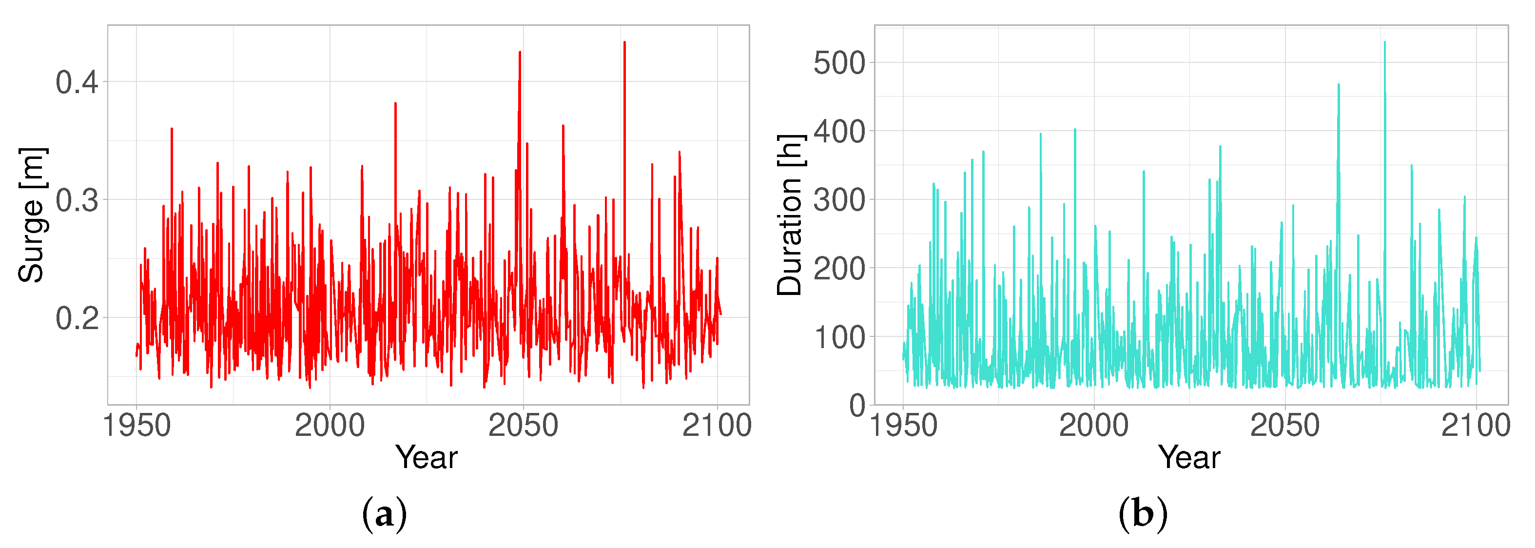
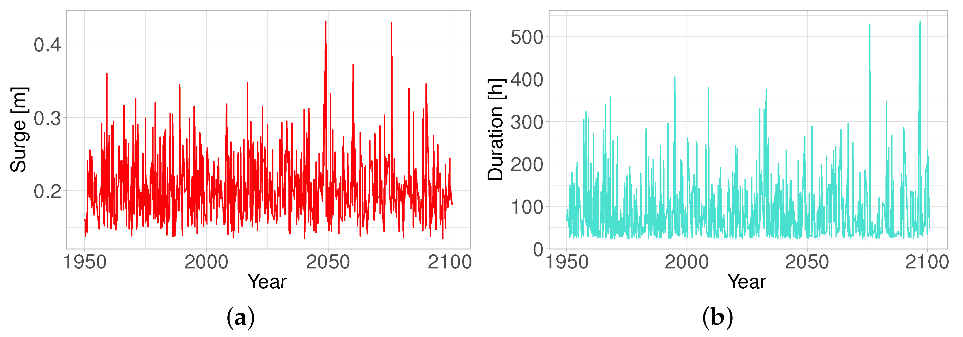
4.1. Process-Based Model

This subsection addresses the results from HYPSE projections at a set of four specific points. These points were selected as representatives of the general behavior of the model at the study area. All four points presented a high variance in $S_p$ and D for the whole period, but they showed a constant moving average throughout time. For instance, the $S_p$ at Tossa (Figure 4) ranged from $0.14$ to 0.43 m, with a mean equal to 0.21 m. The maximum modeled surges had the same order of magnitude as the tidal station measurements. Its D ranged between 25 and 530 h, with a mean equal to 68 h, in the same time period.

However, two spatial clusters can be stated: (i) a northern one from Llanca to Badalona and (ii) a southern one from Badalona to the Ebro Delta. As stated in Section 2, the Northern part of the Catalan Coast was more affected from sharp wind gradients than the South. The central part (Badalona, Figure 5) featured a transition area. At the north, wind stress from N-NW sectors (i.e., Tramontana and Mistral winds) drove surges. Then, $S_p$ at Llanca (Figure 6) peaked above 0.25 m more frequently than at the other points. Whereas $S_p$ values above 0.3 m were uncommon at La Marquesa (15 storms in Figure 7), there were around 50 storms at Llanca and 30 storms at Tossa. Additionally, high $S_p$ events were grouped at specific decades, whilst other decades were relatively calmer, with $S_p$ below 0.25 m at Llanca. These results suggested that the variability of large-scale climate may have a role in the intensity and duration of the events.

Storm duration was more homogeneous along the Catalan coast. However, events above 250 h were more frequent in the North than in the South: around 30 events were above this duration at Llanca and Tossa, whereas the number decreased to 20 events at La Marquesa. Note also that the exceptional storm events in the sample (high $S_p$ and D, as the one around 2075) affected the whole study area. They highlighted an upper bound of what may be possible. However, these rare events were highly uncertain, and they could not be representative of strong conclusions.

The results of the validation will be shown in the next subsection. The empirical PDF (from the measurements) and the fitted PDFs are compared with the method stated in Section 3.3.

4.2. Non-Stationary Statistical Models

This subsection handles the second step in the analysis, showing the results from the fitting of the non-stationary probability distributions. The climate index that presented the strongest influence on the threshold $h_0$ was, by a significant difference, $SC$ (see Figure 8). Therefore, only this one climate index was selected, following the principle of parsimony. Its $C_r=0.134$ was comparable to the $O_{rel}$ of surge levels, which was $0.207$.

The climate index that presented the strongest influence on the frequency parameter $\lambda$ was $SC$. Its $C_r$ was $0.156$, while $\lambda$ in the Catalan coast was of the order of one to 10 storms/year. Hence, $SC$ was related to a higher frequency $\lambda$.

The climate index combination that mostly affected the value of the location parameter $x_0$ of the GPD of $S_p$ was a combination of $\mathrm{NAO}$ and $d^2\mathrm{NAO}$ (see Figure 9). Its $C_r=-0.001$ was significantly smaller than its $O_{rel}=0.207$, exhibiting that a combination of $NAO$ and $d^{2}NAO$ had a small effect on the mean of $S_p$. The BIC indices presented analogous trends to the AIC indices. The climate pattern that mostly affected the value of the location parameter $x_0$ of D was $\mathrm{SC}$ (see Figure 9). Its $C_r=0.038$ was much smaller than its $O_{rel}=4.187$. Thus, the mean value of D was independent of the proposed climate patterns.

In Strategy #1, the climate indices that presented the strongest influence on the value of the scale parameter $\beta$ of $S_p$ were a combination of $d\mathrm{SC}$ and $d^2\mathrm{SC}$ (see Figure 10). Its $C_r=-0.85$ was comparable to its $O_{rel}=0.207$. Thus, negative values of a combination of $d\mathrm{SC}$ and $d^2\mathrm{SC}$ (mainly meaning an accelerating shift of negative $SC$) led to larger variance of $S_p$. The combination of climate indices that presented the strongest influence on the value of the scale parameter $\beta$ of D was $NAO$. Its $C_r=0.16$ was, comparable to $O_{rel}=4.187$. Therefore, positive values of $NAO$ led to a larger variance of D. The modeled $\tau$ from the dependence structure proposed in Lin-Ye et al. [21] is shown in Figure 11. This plot presents discontinuities in time-slices that did not have enough extreme surge events to be fit by a stationary copula. These values of $\tau$ ranged between $0.1$ and $0.37$, thus showing low to moderate correlation.

In Strategy #2, the climate indices that showed the strongest influence on the scale parameters $\beta$ of $S_p$ and D were $EAWR$ and $NAO$, respectively (see Figure 12 and Figure 13). $C_r$ for the $\beta$ of $S_p$ was $0.120$, while $O_{rel}=0.207$ (the same one as for $S_p$ in Strategy #1). $C_r$ was comparable to $O_{rel}$, here. Then, a positive $EAWR$ led to larger variance of $S_p$. $C_r$ for D was $0.071$, while $O_{rel}=4.187$ (the same one as for D in Strategy #1). $C_r$ was significantly smaller than $O_{rel}$, here. Then, the variance of D was not affected by the proposed climate patterns.

The $\tau$ computed with the methodology described in Marra and Radice [41] is shown in Figure 14. It ranged between $0.1$ and $0.26$. There was the same phase at all model points, but the amplitudes depended on the point. The climate index that presented the greatest influence on the copula was $NAO$ (see Figure 13). Its $C_r=-4.104$ was greater than its $O_{rel}=1.193$. Therefore, a negative $NAO$ led to greater dependence between $S_p$ and D.

The VGAM used to estimate all the parameters complied with the corresponding assumptions (see Section 3.2). Finally, the Barcelona tidal gauge was used for the validation. For the years 1993–2016, the Aitchison distance corresponding to $S_p$ was $1.14$. The corresponding Kullback–Leibler divergence was $0.15$. The module of $S_p$ was of the order of one, that meant that the PDFs of the measured and modeled had strong similarity. Then, the statistical characterization of projected $S_p$ resembled that of observed $S_p$, in the years 1993–2016. Regarding the event duration, measured and modeled durations were at the same order of magnitude. On average, the measured surge was above 16 cm at around 275 h/year. The minimum storm surge modeled was around 24 h, and the most extraordinary events lasted for almost 500 h. Please note that the proposed definition was that the surge was above the modeled threshold, which ranged around 15 cm.

5. Discussion

HYPSE outputs represent the general behavior of storm surges at the Catalan cast. Previous research with different GCMs, scenarios, and hydrodynamic models have shown similar trends [13,15]. Modeling surges at the NW Mediterranean requires atmospheric forcings with a relative high horizontal resolution. Hence, GCMs’ usual resolution is insufficient for handling the orographic effects presents in the study Area [73]. In this contribution, the COSMO-CLM model was needed for downscaling the GCM forcings. Otherwise, common extreme wind regimes such as Mistral or Tramontana could not be properly assessed. Extreme winds have a prominent role in the local surge due to wind setup [34,35].

The sensibility analysis on the threshold $h_0$ showed that a $h_0$ equal to the 95th quantile would lead to similar values of D as using the 90th quantile, whereas there would be an insufficient amount of samples to calculate the joint probability density. Therefore, the 90th quantile of $S_p$ can be considered an adequate threshold ($h_0$).

The threshold $h_0$ and the frequency $\lambda$ are directly linked to $SC$. Usually, if the $h_0$ rises, $\lambda$ should decrease, but it seems that $SC$ first leads to a higher $\lambda$, and then, this value is not reduced sufficiently by a rising $h_0$. It can be observed that $NAO$ also has a great influence on $\lambda$ (see Figure 8). It is similar to the Gulf of Lions, where a higher $\lambda$ is reported for negative $NAO$ [74].

$S_p$ and D presented significant variance, but had a constant running mean in the years 1950–2100 (see Figure 4). This is reflected by the results in

Table 1. Most influential climate indices on parameters. The variables are: surge level at the peak of the extreme surge event ($S_p$) and duration of the extreme surge event (D). The climate indices are: North Atlantic oscillation ($NAO$), East Atlantic-West Russian pattern ($EAWR$), and Scandinavian pattern ($SC$). The prefix “d-” means “first time-derivative of”, and the prefix “d2-” means “second time-derivative of”. $C_r$ is a coefficient from the vectorial generalized additive model and can be compared to the relative order of magnitude of the variable to the climate index.

			${\mathit{S}}_{\mathit{p}}$	D
Both strategies	Storm surge threshold	$SC$ ($C_r=0.134$)
	Frequency $\lambda$	$SC$ ($C_r=0.156$)
	Location parameter ($x_0$) of the generalized Pareto distribution		–	–
Strategy #1: Lin-Ye	Scale parameter $\beta$ of the generalized Pareto distribution		$dSC+d^{2}SC$ ($C_r=-0.85$)	$NAO$ ($C_r=0.16$)
Strategy #2: Marra-Radice	$\beta$		$EAWR$ ($C_r=0.120$)	–
	Kendall’s $\tau$ of the copula		$NAO$ ($C_r=-4.104$)

, which shows low dependence on the selected climate patterns for both $S_p$ and D statistical means. Another result for D is that it can take large values of approximately 20 days. This might be caused by the fact that the selected threshold $h_0$, set low to avoid excluding an excessive amount of extreme surge events, had the limitation that on rare occasions, it could be too permissive in the selection of extreme surge events. From Figure 4, it seems that the running variance of $S_p$ and D would be larger from 2030 to 2100. That is, the variance of these two variables seemed to increase with time. This could be explained by the effect of $NAO$, $EAWR$, and $SC$ on the scale parameters $\beta$ of the GPDs of these two variables.

The combination of climate indices that had the most influence on the GPD and copula parameters varied from Strategies #1 to #2 (see Table 1). This might be the effect of full non-stationarity in Strategy #2. In the case of doubt, Strategy #2 should prove more reliable and flexible. Its dependence structure did not depend on time, rather on large-scale climate patterns. Hence, in the case of strong negative $NAO$, there would be more probability of high duration surges jointly with high sea levels at the surge peak. Furthermore, note that, in Strategy #1 (see Figure 9 and Figure 10), the values of AIC are significantly different between the location parameter $x_0$ and the scale parameter $\beta$ of GPD. This does not happen in Strategy #2 (see Figure 12 and Figure 13), where the AIC value for the location parameter $x_0$, the scale parameter $\beta$, and even Kendall’s $\tau$ of the dependence parameter are similar in order of magnitude. This is because, in Strategy #1, a quantile regression VGAM is used to obtain the location parameter $x_0$, while a VGLM is used to obtain the scale parameter $\beta$. In Strategy #2, however, one single type of model, the probit model, characterizes location parameter $x_0$, the scale parameter $\beta$, and the dependence parameter at the same time. The AIC (and the BIC, which produces similar values for this methodology) is an information measure of models. Its value can easily be of different orders of magnitude for different models, while sharing a similar order of magnitude for the same model.

The $\xi$ is always negative in the GPD at these model points, whereas the order of magnitude of the location parameter $x_0$ and the scale parameter $\beta$ of the GPD are similar to each other. Thus, the approximations in Equations (3) and (4) are applicable. A negative shape parameter is related to probability distribution functions that have finite tails, which means that extreme values have a lesser importance in these distributions.

Instead of discussing $x_0$ and $\beta$, it is equivalent to talk about the statistical mean and variance, which are more easily related to physical phenomena. The mean of $S_p$ and the variance of D (in both strategies) are not affected by $NAO$, $EAWR$, nor $SC$ (see Table 1), the same way that the scale parameter $x_0$ of the GPD is constant. However, there is some evidence of the effect of an external forcing, possibly another climate pattern. This is out of the scope of this paper, but could be explored in future work.

The temporal dynamics of $SC$ seems to be key to the variance of $S_p$, in Strategy #1. It can be deduced that periods of extraordinary positive gradients of $SC$ would intensify the variability of $S_p$. Moreover, a positive $NAO$ would increase the variability of D. It should be noted that a positive velocity of $SC$ leads to extreme wave storm total energy [21], and a negative $NAO$ is linked to large SWH [23]. Therefore, periods with these characteristics are especially prone to damage caused by the joint action of wave storms and extreme surge events. Other external enhancers to the damage caused by $S_p$ and D are coastal erosion and reduction of the beach width. The reduction of the beach width occurs by modifying the responses of the coast to the propagation and intensification of the extreme surge events over a long time.

The correlation between wave storms and extreme surge events has not been considered, as the dependence density between wave storms and extreme surge events in the Catalan coast is not entirely clear, in this case. This correlation might depend on the directionality and fetch of the wave-storm [75,76]. The combined action of storm surges and wind waves may drive increased coastal water levels [77], even under moderate return periods. Furthermore, if adding sea level rise due to global warming, then coastal structures’ vulnerability is even more exacerbated [33,78]. Hence, it may be useful to find consistent relationships between the synoptic patterns and the main hydrodynamic drivers. Such characterization may serve to create design scenarios that would address moderate waves and surges, jointly with sea level rise. These scenarios may be more frequent (and, probably, more harmful) than high return period wave storms and/or surges.

Incidentally, the relevant effect of $NAO$ on $S_p$ coincides with existent literature, which states that the observed surge levels increase in the Catalan coast for negative $NAO$, because this condition causes a shift of atmospheric storm tracks towards lower latitudes [28,79]. High observed surge levels are also reported in the Gulf of Lions, for negative $NAO$ [80].

$SC$ does not present the same relevance in Strategy #2, where it is $EAWR$ that has the strongest influence on the variance of $S_p$. Positive $EAWR$ leads to higher variance of D. Additionally, while in Strategy #1, $NAO$ is an influential climate index on the variance of D, in Strategy #2, the variance of D does not depend on any of the proposed climate patterns. It is possible that $SC$ lost its influence in a non-stationary framework such as Strategy #2, where a wider time window is selected.

The Gumbel copula family, which describes the joint probability density among $S_p$ and D, is symmetric and has its own limitations [81]. However, due to the complexity of the non-stationary model, a symmetric model allows for a simpler model, whereas some main results, such as the influence of climate patterns on GPD and copula parameters, can be considerably close to reality, despite this simplification.

Kendall’s $\tau$, for both strategies, is below $0.37$. It ranges from low to moderate (see Figure 11 and Figure 14) and has constant moving means over time. In Strategy #2, the effect of $NAO$ on $\tau$ at all these model points is demonstrated and is evident, as all the time series of $\tau$ coincide closely in phase. Specifically, a negative $NAO$ leads to higher dependence among $S_p$ and D. The coincidence in phase can also be seen in Strategy #1, where $\tau$ is not related to any climate pattern. The $\tau$ in Strategy #1 shows more frequent fluctuations than the $\tau$ in Strategy #2. Moreover, both figures show that the Tossa, Lloret, and Badalona model points denote greater variance. This is evident from the amplitude of the time series, while Llanca and Marquesa present smaller amplitudes of $\tau$. The main reason for this might be the way that the low-sea level pressures and the extreme wind regime happen in this study area. Cyclogenesis and propagation of such storm surges are the driving processes. It seems that, in the northern part of the Catalan Coast, stronger surges and winds are propagated. The surges that occur in the southern part of the Catalan Coast come from milder wind fields and sea level pressure anomalies. Hence, they tend to have lower anomalies.

6. Conclusions

A hybrid approach was used to characterize extreme surge events at the Catalan coast. It consisted of a process-based model and a statistical model. The process-based model generated projected surge levels for the period 1950-2100, under the climate change scenario RCP8.5. Extreme surge events were extracted from this time series through a non-stationary threshold $h_0$, which defined a $\lambda$ (frequency of a Poisson’s process) of extreme events and produced the variables $S_p$ (maximum surge level) and D (duration), describing them.

A statistical model was proposed to characterize the maximum surge level and duration with GPDs and their joint probability density with Gumbel-type Archimedean copulas. This statistical model also relates these variables to indices of three climate patterns and their first two time-derivatives: $NAO$, $EAWR$, and $SC$. Two different strategies were proposed for the statistical model. These two strategies were based on the bivariate copula model methodology developed in Lin-Ye et al. [21] (Strategy #1) and its non-stationary version Marra and Radice [41] (strategy #2), each. The strategies shared all steps except the estimation and establishment of the relationship of the scale parameter $\beta$ of the GPD and Kendall’s $\tau$ to the climate indices. Strategy #1 estimates $\beta$ through a VGLM and characterized the joint probability density by concatenating standard stationary Archimedean copulas. Strategy #2 integrated the estimation of $\beta$ along with the non-stationary Archimedean copula, within a bivariate probit model.

The results showed how $SC$ and its dynamics strongly influenced the threshold and the event frequency. Both parameters increased with positive $SC$. Maximum surge level and duration had a constant moving mean from 1950 to 2100, while their running variance increased with time. The constant moving mean of the two variables could be explained by the fact that they were not sensitive to the proposed climate patterns. The increase in the running variance might be due to the effect of different combinations of climate patterns on the scale parameter $\beta$ of the GPD used to fit each variable.

The location parameter $x_0$ of the GPD was not influenced by any of the proposed climate indices. According to Strategy #1, a combination of rapidly shifting negative $SC$ led to an increase in the variance of the maximum surge level, whereas the variance of duration increased with positive $NAO$. In Strategy #2, the variance of maximum surge level increased with positive $EAWR$ and the variance of duration was independent of the proposed climate patterns.

In both strategies, the values of Kendall’s $\tau$ of the dependence parameter were below $0.4$, ranging from low to medium dependence among maximum surge level and duration. The $\tau$ in Strategy #1 had a constant trend and was similar for all locations. $\tau$ in Strategy #2 presented the same phase for all model points, but provided different amplitudes for each point. In this strategy as well, Kendall’s $\tau$ of the two variables increased with negative $NAO$.

The big picture of the influence of the proposed climate patterns was that $NAO$ and $SC$ had a strong influence on the threshold $h_0$ and the frequency $\lambda$ (according to Strategy #1), the variances of the maximum surge level and duration, and (according to Strategy #2) the joint probability density. The knowledge about this relationship between $NAO$ and $SC$ with maximum surge level and duration could help with predicting changes in maximum surge level and duration, with previous knowledge about these two climate patterns. Special attention must be paid to Strategy #2, which was the fully non-stationary model. This could improve the design of coastal structures that have to withstand the action caused by extreme surge events, as well as protection measures for mitigating coastal risk levels.

References

1. Bolaños, R.; Jordà, G.; Cateura, J.; López, J.; Puigdefàbregas, J.; Gómez, J.; Espino, M. The XIOM: 20 years of a regional coastal observatory in the Spanish Catalan coast. J. Mar. Syst. 2009, 77, 237–260. [Google Scholar] [CrossRef] [Green Version]
2. Soomere, T.; Pindsoo, K. Spatial variability in the trends in extreme storm surges and weekly-scale high water levels in the eastern Baltic Sea. Cont. Shelf Res. 2016, 115, 53–64. [Google Scholar] [CrossRef]
3. Brown, J.D.; Spencer, T.; Moeller, I. Modeling storm surge flooding of an urban area with particular reference to modeling uncertainties: A case study of Canvey Island, United Kingdom. Water Resour. Res. 2007, 43. [Google Scholar] [CrossRef] [Green Version]
4. Hinkel, J.; Lincke, D.; Vafeidis, A.T.; Perrette, M.; Nicholls, R.J.; Tol, R.S.J.; Marzeion, B.; Fettweis, X.; Ionescu, C.; Levermann, A. Coastal flood damage and adaptation costs under 21st century sea-level rise. Proc. Natl. Acad. Sci. USA 2014, 111, 3292–3297. [Google Scholar] [CrossRef] [PubMed] [Green Version]
5. Zhang, H.; Cheng, W.C.; Qiu, X.X.; Feng, X.B.; Gong, W.P. Tide-surge interaction along the east coast of the Leizhou Peninsula, South China Sea. Cont. Shelf Res. 2017, 142, 32–49. [Google Scholar] [CrossRef]
6. Ullmann, A.; Pirazzoli, P.A.; Tomasin, A. Sea surges in Camargue: Trends over the 20th century. Cont. Shelf Res. 2007, 27, 922–934. [Google Scholar] [CrossRef]
7. Staneva, J.; Wahle, K.; Koch, W.; Behrens, A.; Fenoglio-Marc, L.; Stanev, E.V. Coastal flooding: Impact of waves on storm surge during extremes - a case study for the German Bight. Nat. Hazards Earth Sys. Sci. 2016, 16, 2373–2389. [Google Scholar] [CrossRef] [Green Version]
8. Sánchez-Arcilla, A.; García-León, M.; Gracia, V.; Devoy, R.; Stanica, A.; Gault, J. Managing coastal environments under climate change: Pathways to adaptation. Sci. Total Environ. 2016, 572, 1336–1352. [Google Scholar] [CrossRef] [Green Version]
9. Krien, Y.; Testut, L.; Islam, A.K.M.S.; Bertin, X.; Durand, F.; Mayet, C.; Tazkia, A.R.; Becker, M.; Calmant, S.; Papa, F.; et al. Towards improved storm surge models in the northern Bay of Bengal. Cont. Shelf Res. 2017, 135, 58–73. [Google Scholar] [CrossRef]
10. Grases, A.; Gracia, V.; García-León, M.; Lin-Ye, J.; Sierra, J.P. Coastal Flooding and Erosion under a Changing Climate: Implications at a Low-Lying Coast (Ebro Delta). Water 2020, 12, 346. [Google Scholar] [CrossRef] [Green Version]
11. Silva, A.T.; Naghettini, M.; Portela, M.M. On some aspects of peaks-over-threshold modeling of floods under nonstationarity using climate covariates. Stoch. Environ. Res. Risk Assess. 2016, 30, 207–224. [Google Scholar] [CrossRef]
12. Du, T.; Xiong, L.H.; Xu, C.Y.; Gippel, C.J.; Guo, S.; Liu, P. Return period and risk analysis of nonstationary low-flow series under climate change. J. Hydrol. 2015, 527, 234–250. [Google Scholar] [CrossRef] [Green Version]
13. Vousdoukas, M.I.; Voukouvalas, E.; Annunziato, A.; Giardino, A.; Feyen, L. Projections of extreme storm surge levels along Europe. Clim. Dyn. 2016, 1–20. [Google Scholar] [CrossRef] [Green Version]
14. Conte, D.; Lionello, P. Characteristics of large positive and negative surges in the Mediterranean Sea and their attenuation in future climate scenarios. Glob. Planet. Chang. 2013, 111, 159–173. [Google Scholar] [CrossRef]
15. Marcos, M.; Jordà, G.; Gomis, D.; Pérez, B. Changes in storm surges in southern Europe from a regional model under climate change scenarios. Glob. Planet. Chang. 2011, 77, 116–128. [Google Scholar] [CrossRef]
16. Barnston, A.G.; Livezey, R.E. Classification, Seasonality and Persistence of Low-Frequency Atmospheric Circulation Patterns. Mon. Weather Rev. 1987, 115, 1083–1126. [Google Scholar] [CrossRef]
17. Hurrell, J.W.; Deser, C. North Atlantic climate variability: The role of the North Atlantic Oscillation. J. Marine Syst. 2009, 78, 28–41. [Google Scholar] [CrossRef]
18. Lionello, P.; Malanotte-Rizzoli, P.; Boscolo, R. Mediterranean Climate Variability; Elsevier: Amsterdam, The Netherlands, 2006; Volume 4. [Google Scholar]
19. Lionello, P.; Sanna, A. Mediterranean wave climate variability and its links with NAO and Indian Monsoon. Clim. Dyn. 2005, 25, 611–623. [Google Scholar] [CrossRef]
20. Lionello, P.; Cogo, S.; Galati, M.; Sanna, A. The Mediterranean surface wave climate inferred from future scenario simulations. Glob. Planet. Change 2008, 63, 152–162. [Google Scholar] [CrossRef]
21. Lin-Ye, J.; García-León, M.; Gràcia, V.; Ortego, M.I.; Lionello, P.; Sánchez-Arcilla, A. Multivariate statistical modeling of future marine storms. Appl. Ocean Res. 2017, 65, 192–205. [Google Scholar] [CrossRef] [Green Version]
22. Trigo, R.M.; Osborn, T.J.; Corte-Real, J.M. The North Atlantic Oscillation influence on Europe: Climate impacts and associated physical mechanisms. Clim. Res. 2002, 20, 9–17. [Google Scholar] [CrossRef]
23. Ulbrich, U.; Lionello, P.; Belusic, D.; Jacobeit, J.; Knippertz, P.; Kuglitsch, F.G.; Leckebusch, G.C.; Luterbacher, J.; Maugeri, M.; Maheras, P.; et al. 5—Climate of the Mediterranean: Synoptic Patterns, Temperature, Precipitation, Winds, and Their Extremes. In The Climate of the Mediterranean Region; Lionello, P., Ed.; Elsevier: Oxford, UK, 2012; pp. 301–346. [Google Scholar] [CrossRef]
24. Lionello, P.; Galati, M.B. Links of the significant wave height distribution in the Mediterranean sea with the Northern Hemisphere teleconnection patterns. Adv. Geosci. 2008, 17, 13–18. [Google Scholar] [CrossRef] [Green Version]
25. Tsimplis, M.N.; Shaw, A.G.P.; Flather, R.A.; Woolf, D.K. The influence of the North Atlantic Oscillation on the sea-level around the northern European coasts reconsidered: The thermosteric effects. Philos. Trans. A Math. Phys. Eng. Sci. 2006, 364, 845–856. [Google Scholar] [CrossRef] [PubMed]
26. Woodworth, P.; Flather, R.A.; Williams, J.A.; Wakelin, S.L.; Jevrejeva, S. The dependence of U.K. extreme sea levels and storm surges on the North Atlantic Oscillation. Cont. Shelf Res. 2007, 27, 935–946. [Google Scholar] [CrossRef]
27. Cid, A.; Menéndez, M.; Castanedo, S.; Abascal, A.J.; Méndez, F.J.; Medina, R. Long-term changes in the frequency, intensity and duration of extreme storm surge events in southern Europe. Clim. Dyn. 2016, 46, 1503–1516. [Google Scholar] [CrossRef]
28. Lionello, P.; Conte, D.; Marzo, L.; Scarascia, L. The contrasting effect of increasing mean sea level and decreasing storminess on the maximum water level during storms along the coast of the Mediterranean Sea in the mid 21st century. Glob. Planet. Chang. 2016, 151, 80–91. [Google Scholar] [CrossRef]
29. Wadey, M.P.; Haigh, I.D.; Brown, J.M. A century of sea level data and the UK’s 2013/14 storm surges: An assessment of extremes and clustering using the Newlyn tide gauge record. Ocean Sci. 2014, 10, 1031–1045. [Google Scholar] [CrossRef] [Green Version]
30. Wakelin, S.L.; Woodworth, P.L.; Flather, R.A.; Williams, J.A. Sea-level dependence on the NAO over the NW European Continental Shelf. Geophy. Res. Lett. 2003, 30. [Google Scholar] [CrossRef]
31. Hemer, M.A.; Trenham, C.E. Evaluation of a CMIP5 derived dynamical global wind wave climate model ensemble. Ocean Model. 2016, 103, 190–203. [Google Scholar] [CrossRef] [Green Version]
32. Trenberth, K.; Fasullo, J.; Shepherd, T. Attribution of climate extreme events. Nat. Clim. Chang. 2015, 5, 725–730. [Google Scholar] [CrossRef]
33. Campos, Á.; García-Valdecasas, J.M.; Molina, R.; Castillo, C.; Álvarez-Fanjul, E.; Staneva, J. Addressing Long-Term Operational Risk Management in Port Docks under Climate Change Scenarios—A Spanish Case Study. Water 2019, 11, 2153. [Google Scholar] [CrossRef] [Green Version]
34. Marcos, M.; Tsimplis, M.N.; Shaw, A.G.P. Sea level extremes in southern Europe. J. Geophys. Res. Oceans 2009, 114. [Google Scholar] [CrossRef] [Green Version]
35. Lionello, P.; Conte, D.; Reale, M. The effect of cyclones crossing the Mediterranean region on sea level anomalies on the Mediterranean Sea coast. Nat. Hazards Earth Syst. Sci. 2019, 19, 1541–1564. [Google Scholar] [CrossRef] [Green Version]
36. De Michele, C.; Salvadori, G.; Passoni, G.; Vezzoli, R. A multivariate model of sea storms using copulas. Coast. Eng. 2007, 54, 734–751. [Google Scholar] [CrossRef]
37. Wahl, T.; Mudersbach, C.; Jensen, J. Assessing the hydrodynamic boundary conditions for risk analyses in coastal areas: A multivariate statistical approach based on Copula functions. Nat. Hazards Earth Syst. Sci. 2012, 12, 495–510. [Google Scholar] [CrossRef] [Green Version]
38. Corbella, S.; Stretch, D.D. Simulating a multivariate sea storm using Archimedean copulas. Coast. Eng. 2013, 76, 68–78. [Google Scholar] [CrossRef]
39. Masina, M.; Lamberti, A.; Archetti, R. Coastal flooding: A copula based approach for estimating the joint probability of water levels and waves. Coast. Eng. 2015, 97, 37–52. [Google Scholar] [CrossRef]
40. Woollings, T.; Blackburn, M. The North Atlantic jet stream under climate change and its relation to the NAO and EA patterns. J. Clim. 2012, 25, 886–902. [Google Scholar] [CrossRef] [Green Version]
41. Marra, G.; Radice, R. Bivariate copula additive models for location, scale and shape. Comp. Stat. Data Anal. 2017, 112, 99–113. [Google Scholar] [CrossRef]
42. Stocker, T.; Qin, D.; Plattner, G.K.; Tignor, M.; Allen, S.; Boschung, J.; Nauels, A.; Xia, Y.; Bex, V.; Midgley, P. IPCC, 2013: Summary for Policymakers. In Climate Change 2013: The Physical Science Basis. Contribution of Working Group I to the Fifth Assessment Report of the Intergovernmental Panel on Climate Change; Cambridge University Press: Cambridge, UK; New York, NY, USA, 2013. [Google Scholar]
43. Scoccimarro, E.; Gualdi, S.; Bellucci, A.; Sanna, A.; Fogli, P.G.; Manzini, E.; Vichi, M.; Oddo, P.; Navarra, A. Effects of Tropical Cyclones on Ocean Heat Transport in a High-Resolution Coupled General Circulation Model. J. Clim. 2011, 24, 4368–4384. [Google Scholar] [CrossRef] [Green Version]
44. Butterworth, S. On the theory of filter amplifiers. Wireless Eng. 1930, 7, 536–541. [Google Scholar]
45. Rockel, B.; Will, A.; Hense, A. The Regional Climate Model COSMO-CLM (CCLM). Meteorol. J. 2008, 17, 347–348. [Google Scholar] [CrossRef]
46. Lionello, P.; Mufato, R.; Tomasin, A. Sensitivity of free and forced oscillations of the Adriatic Sea to sea level rise. Clim. Res. 2005, 29, 23–29. [Google Scholar] [CrossRef] [Green Version]
47. Egozcue, J.J.; Pawlowsky-Glahn, V.; Ortego, M.I.; Tolosana-Delgado, R. The effect of scale in daily precipitation hazard assessment. Nat. Hazards Earth Sys. Sci. 2006, 6, 459–470. [Google Scholar] [CrossRef] [Green Version]
48. Yee, T.W.; Wild, C.J. Vector Generalized Additive Models. J. R. Stat. Soc. Series B. Methodol. 1996, 58, 481–493. [Google Scholar] [CrossRef]
49. Fessler, J. Nonparametric fixed-interval smoothing with vector splines. Signal Process. IEEE Trans. 1991, 39, 852–859. [Google Scholar] [CrossRef] [Green Version]
50. Hastie, T.J.; Tibshirani, R.J. Generalized Additive Models; CRC Press: Boca Raton, FL, USA, 1990; Volume 43. [Google Scholar]
51. Rigby, R.A.; Stasinopoulos, D.M. Generalized additive models for location, scale and shape. J. R. Stat. Soc. Series C Appl. Stat. 2005, 54, 507–554. [Google Scholar] [CrossRef] [Green Version]
52. Yee, T.W.; Stephenson, A.G. Vector generalized linear and additive extreme value models. Extremes 2007, 10, 1–19. [Google Scholar] [CrossRef]
53. Coles, S. An introduction to Statistical Modeling of Extreme Values; Springer: London, UK, 2001; pp. 801–804. [Google Scholar]
54. Koenker, R. Quantile Regression; Econometric Society Monographs; Cambridge University Press: Cambridge, UK, 2005. [Google Scholar]
55. Northrop, P.J.; Jonathan, P. Threshold modeling of spatially dependent non-stationary extremes with application to hurricane-induced wave heights. Environmetrics 2011, 22, 799–809. [Google Scholar] [CrossRef]
56. Jonathan, P.; Ewans, K.; Randell, D. Joint modeling of extreme ocean environments incorporating covariate effects. Coast. Eng. 2013, 79, 22–31. [Google Scholar] [CrossRef] [Green Version]
57. Akaike, H. Factor analysis and AIC. Psychometrika 1987, 52, 317–332. [Google Scholar] [CrossRef]
58. Tamura, Y.; Sato, T.; Ooe, M.; Ishiguro, M. A procedure for tidal analysis with a Bayesian information criterion. Geophys. J. Int. 1991, 104, 507–516. [Google Scholar] [CrossRef] [Green Version]
59. Sklar, A. Fonctions dé Repartition à n Dimension et Leurs Marges; Université Paris 8: Paris, France, 1959. [Google Scholar]
60. Nelsen, R. An Introduction to Copulas; Springer Science & Business Media: New York, NY, USA, 2007. [Google Scholar]
61. Okhrin, O.; Okhrin, Y.; Schmid, W. On the structure and estimation of hierarchical Archimedean copulas. J. Econom. 2013, 173, 189–204. [Google Scholar] [CrossRef]
62. Lin-Ye, J.; García-León, M.; Gràcia, V.; Sánchez-Arcilla, A. A multivariate statistical model of extreme events: An application to the Catalan coast. Coast. Eng. 2016, 117, 138–156. [Google Scholar] [CrossRef] [Green Version]
63. Kendall, M. A new measure of rank correlation. Biometrika 1937, 6, 83–93. [Google Scholar]
64. Salvadori, G.; De Michele, C.; Durante, F. On the return period and design in a multivariate framework. Hydrol. Earth Syst. Sci. 2011, 15, 3293–3305. [Google Scholar] [CrossRef] [Green Version]
65. Joe, H. Dependence Modeling with Copulas; Chapman and Hall/CRC: London, UK, 2014. [Google Scholar]
66. Salvadori, G.; De Michele, C.; Kottegoda, N.T.; Rosso, R. Extremes in Nature: An Approach Using Copulas; Springer Science & Business Media: Amsterdam, The Netherlands, 2007; Volume 56. [Google Scholar]
67. Kullback, S. Information Theory and Statistics; Courier Corporation: Chelmsford, MA, USA, 1997. [Google Scholar]
68. Aitchison, J. On criteria for measures of compositional difference. Math. Geol. 1992, 24, 365–379. [Google Scholar] [CrossRef]
69. Pawlowsky-Glahn, V.; Egozcue, J.J.; Tolosana-Delgado, R. Modeling and Analysis of Compositional Data; John Wiley & Sons: Hoboken, NJ, USA, 2015. [Google Scholar]
70. Aitchison, J. The statistical analysis of compositional data. J. R. Stat. Soc. Ser. B Methodol. 1982, 44, 139–177. [Google Scholar] [CrossRef]
71. Egozcue, J.J.; Pawlowsky-Glahn, V.; Mateu-Figueras, G.; Barceló-Vidal, C. Isometric logratio transformations for compositional data analysis. Math. Geol. 2003, 35, 279–300. [Google Scholar] [CrossRef]
72. Pawlowsky-Glahn, V.; Egozcue, J.J. Geometric approach to statistical analysis on the simplex. Stoch. Environ. Res. Risk Assess. 2001, 15, 384–398. [Google Scholar] [CrossRef]
73. Obermann-Hellhund, A.; Conte, D.; Somot, S.; Torma, C.Z.; Ahrens, B. Mistral and Tramontane wind systems in climate simulations from 1950 to 2100. Clim. Dyn. 2018, 50, 693–703. [Google Scholar] [CrossRef] [Green Version]
74. Ullmann, A.; Moron, V. Weather regimes and sea surge variations over the Gulf of Lions (French Mediterranean coast) during the 20th century. Int. J. Clim. 2008, 28, 159–171. [Google Scholar] [CrossRef]
75. Bertin, X.; Li, K.; Roland, A.; Bidlot, J.R. The contribution of short-waves in storm surges: Two case studies in the Bay of Biscay. Cont. Shelf Res. 2015, 96, 1–15. [Google Scholar] [CrossRef]
76. Brown, J.M.; Wolf, J. Coupled wave and surge modeling for the eastern Irish Sea and implications for model wind-stress. Cont. Shelf Res. 2009, 29, 1329–1342. [Google Scholar] [CrossRef] [Green Version]
77. Marcos, M.; Rohmer, J.; Vousdoukas, M.I.; Mentaschi, L.; Le Cozannet, G.; Amores, A. Increased Extreme Coastal Water Levels Due to the Combined Action of Storm Surges and Wind Waves. Geophys. Res. Lett. 2019, 46, 4356–4364. [Google Scholar] [CrossRef] [Green Version]
78. Mase, H.; Tsujio, D.; Yasuda, T.; Mori, N. Stability analysis of composite breakwater with wave-dissipating blocks considering increase in sea levels, surges and waves due to climate change. Ocean Eng. 2013, 71, 58–65. [Google Scholar] [CrossRef] [Green Version]
79. Tsimplis, M.N.; Álvarez-Fanjul, E.; Gomis, D.; Fenoglio-Marc, L.; Pérez, B. Mediterranean Sea level trends: Atmospheric pressure and wind contribution. Geophys. Res. Lett. 2005, 32, L20602. [Google Scholar] [CrossRef]
80. Ullmann, A.; Pirazzoli, P.; Moron, V. Sea surges around the Gulf of Lions and atmospheric conditions. Glob. Planet. Chang. 2008, 63, 203–214. [Google Scholar] [CrossRef]
81. Vanem, E. Joint statistical models for significant wave height and wave period in a changing climate. Mar. Struct. 2016, 49, 180–205. [Google Scholar] [CrossRef]
Figure 1. (a) North-Western Mediterranean Sea. The red line rectangle encloses the study area; (b) Zoom at the Catalan coast. The red dots are the available stations from the barotropic model, whereas the yellow rhombus is the Barcelona tidal gauge (TG-BCN; REDMARvalidation station). PROF are the isobaths (in meters). Water depth in meters.
Water 12 00472 g001
Figure 2. Flowchart of the proposed hybrid methodology to model the extreme surge events. The steps of the hybrid methodology are: (1) a process-based model, (2) a statistical model, and (3) validation of the statistical model. The statistical model (a bivariate copula model) is fed by the output data from the process-based model. The statistical model can adopt two different strategies, with either a pseudo-non-stationary and a non-stationary computation of the distribution parameters. Rectangles refer to data and rhombs to processes. CMCC-CM5, Centro Euro-Mediterraneo sui Cambiamenti Climatici Climate Model; GPD, Generalized Pareto Distribution; VGAM, Vectorial Generalized Additive Model; VGLM, Vectorial Generalized Linear Model.
Water 12 00472 g002
Figure 3. Definition of variables for a single extreme surge event. The red solid time series represent the surge. The discontinuous red line is the threshold. The blue dot shows the maximum level in the event ( S p ). The event has an intermediate calm period of less than 72 h.
Water 12 00472 g003
Figure 4. Descriptive plots of the two surge components at the N-2 Tossa model point (period from 1950–2100). Data extracted from the barotropic model. (a) Continuous red line: surge-level at the peak of the extreme surge event ( S p , in meters); (b) continuous cyan line: duration of the extreme surge event (D, in hours).
Water 12 00472 g004
Figure 5. Descriptive plots of the two surge components at the N-5 Badalona model point (period from 1950–2100). Data extracted from the barotropic model. (a) Continuous red line: surge-level at the peak of the extreme surge event ( S p , in meters); (b) continuous cyan line: Duration of the extreme surge event (D, in hours).
Water 12 00472 g005
Figure 6. Descriptive plots of the two surge components at the N-1 Llanca model point (period from 1950–2100). Data extracted from the barotropic model. (a) Continuous red line: surge level at the peak of the extreme surge event ( S p , in meters); (b) continuous cyan line: duration of the extreme surge event (D, in hours).
Water 12 00472 g006
Figure 7. Descriptive plots of the two surge components at the N-7 Marquesa model point (period from 1950–2100). Data extracted from the barotropic model. (a) Continuous red line: surge-level at the peak of the extreme surge event ( S p , in meters); (b) continuous cyan line: duration of the extreme surge event (D, in hours).
Water 12 00472 g007
Figure 8. Akaike Information Criterion (AIC) indices common to both strategies, since they share the same structure of threshold and frequency of extreme surge events. They show the goodness-of-fit of the different combinations of climate indices: North Atlantic oscillation ( N A O ), East Atlantic-West Russian pattern ( E A W R ), and Scandinavian pattern ( S C ). (a) Threshold of the extreme surge event ( h 0 ) and (b) frequency of extreme surge events ( λ ). The prefix “d-” means “first time-derivative of”, and the prefix “d2-” means “second time-derivative of”. The discontinuous red line shows the selected combination of climate patterns in (a) h 0 and (b) λ .
Water 12 00472 g008
Figure 9. Akaike Information Criterion (AIC) indices common to both strategies, since they share the same structure of the location parameters. They compare the effect of different climate indices: North Atlantic oscillation ( N A O ), East Atlantic-West Russian pattern ( E A W R ), and Scandinavian pattern ( S C ) on the location parameter x 0 of a generalized Pareto distribution fit to (a) the surge level at the peak of the extreme surge event ( S p ) and (b) the duration of the extreme surge event (D). The prefix “d-” means “first time-derivative of”, and the prefix “d2-” means “second time-derivative of”. The discontinuous red line shows the selected combination of climate patterns on x 0 .
Water 12 00472 g009
Figure 10. Strategy #1. Akaike Information Criterion (AIC) indices. They compare the effect of different climate indices: North Atlantic oscillation ( N A O ), East Atlantic-West Russian pattern ( E A W R ), and Scandinavian pattern ( S C ) on the scale parameter β of a generalized Pareto distribution fit to (a) the surge level at the peak of the extreme surge event ( S p ) and (b) the duration of the extreme surge event (D). The prefix “d-” means “first time-derivative of”, and the prefix “d2-” means “second time-derivative of”. The discontinuous red line shows the selected combination of climate patterns on β .
Water 12 00472 g010
Figure 11. Strategy #1. Kendall’s τ s of the dependence parameter of a Gumbel Archimedean copula at the different model points. Each color line represents a node from Figure 1. This plot presents discontinuities in time-slices that do not have enough extreme surge events to be fit by a stationary copula.
Water 12 00472 g011
Figure 12. Strategy #2. Akaike Information Criterion (AIC) indices. They compare the effect of different climate indices: North Atlantic oscillation ( N A O ), East Atlantic-West Russian pattern ( E A W R ), and Scandinavian pattern ( S C ) on the scale parameter β of a generalized Pareto distribution fit to (a) the surge level at the peak of the extreme surge event ( S p ) and (b) the duration of the extreme surge event (D). The prefix “d-” means “first time-derivative of”, and the prefix “d2-” means “second time-derivative of”. The discontinuous red line shows the selected combination of climate patterns on β .
Water 12 00472 g012
Figure 13. Strategy #2. Akaike Information Criterion (AIC) indices. They compare the effect of different climate indices: North Atlantic oscillation ( N A O ), East Atlantic-West Russian pattern ( E A W R ), and Scandinavian pattern ( S C ) on Kendall’s τ of the dependence parameter of a Gumbel Archimedean copula. The discontinuous red line shows the selected combination of climate patterns on τ .
Water 12 00472 g013
Figure 14. Strategy #2. Dependence parameter τ of the Gumbel Archimedean copula at different model points, under the climate change scenario RCP8.5. Each color line represents a node from Figure 1.
Water 12 00472 g014