Improved Planning of Energy Recovery in Water Systems Using a New Analytic Approach to PAT Performance Curves

Abstract

The use of pumps working as turbines (PATs) to improve the energy efficiency of water networks has been studied in the last years. This recovery system is justified due to a low investment contrasting with the capacity to take advantage in certain points with low and medium recoverable heads. Analyses of water systems using simulation software and/or optimization algorithms need the characteristic curves (head and efficiency) of the machines, which should be known with minor error by the water managers. The knowledge of the best efficiency point (BEP) as a turbine is one of the major limitations when the user wants to choose PATs. In this sense, the present research defines new approach equations to estimate the BEP of the PAT, as well as to predict the characteristic curves, comparing the results with the rest of the published methods. The comparison demonstrated that the new proposal reduced the error indexes, improved the R² and increased the accuracy of the error ellipse using an experimental database of 181 different PATs.

1. Introduction

Energy analyses are crucial in water networks when water managers want to apply measurements to improve the sustainability in water systems [1]. One of the different considerations in order to improve the efficiency, and therefore, the sustainability of such systems is the use of microhydropower machines, which take advantage of excess in the pressure. Usually, the pressure, which is not necessary, is dissipated with pressure reduction valves in the network to transform the hydraulic energy to electrical energy [2,3]. Many researches justified the advantage of using pumps working as turbines (PATs) in different water systems (i.e., supply, irrigation and wastewater treatment), since these hydraulic machines have a low investment, as well as the high availability of pump factories [4,5,6]. These proposals were applied at different case studies [7,8,9].

The major challenges of the PATs analyses are: (i) to choose the necessary pump when the available recovered head as a function of flow over time is known; (ii) to predict the operation point of the PAT ($\mathrm{i}.\mathrm{e}., Q, H$ and $\eta$) when the pump is selected and (iii) to estimate the characteristic, efficiency and runaway curves in order to use in the simulation and optimization algorithms. These simulations enable to quantify the recovered energy, and therefore, the improvement of the sustainability in the water systems [10,11,12].

Although there are different methods to approach tasks (ii) and (iii) described in the previous paragraph, the majority of them use a low number of experimental data, and therefore, the committed error is high [13,14]. In this research line, the present research is focused on establishing a new analytical approach, to improve the prediction of the PAT parameters and on the simulation and energy analyses of the water systems. The research contains a deep review of experimental data of PATs that were already published (Figure 1). The database contains a high number of experimental uses; particularly, the research used 181 different PATs, 60% higher than previous studies [12]. The specific speed of the used machine was between 5.09 and 219.09 (m, kW).

The research presents as a novelty the enumeration of a new approach to predict the operation point of the machine acting as a turbine when the BEP parameters ($\mathrm{i}.\mathrm{e}., Q, H$ and $\eta$) in pumping mode are known. The proposed method was compared with the rest of the published methods, improving the error indexes and regression values, as well as the uncertainty ellipse prediction [15]. Besides, the research also presents empirical expressions to estimate the characteristic curves (head, power and efficiency) as functions of the flow considering the BEP conditions. These new equations are compared with the rest of expressions, which have already been published, lowering prediction uncertainty and, therefore, improving the results of energy analysis when water managers develop simulations and optimization algorithms.

2. Materials and Methods

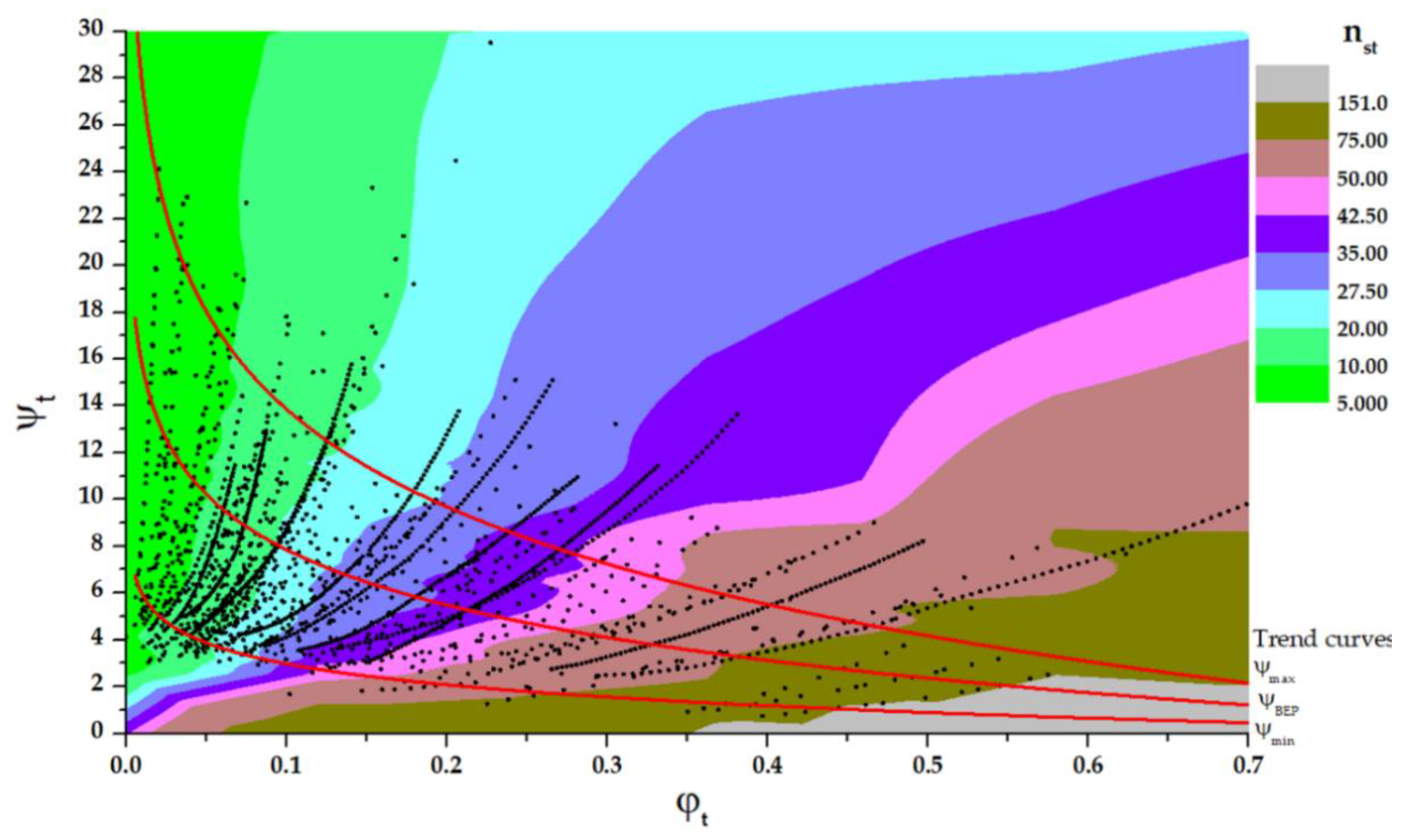
2.1. Definition of the Characteristic Numbers of PATs

The main curves of a PAT for modelling a hydraulic machine in a hydraulic system are: head-discharge curve (Q-H), efficiency curve (Q-$\eta$) and runaway curve when the machine operates without load as well as the curve (Q-H) when the rotational speed of the machine is zero (Figure 2). The knowledge of these curves enables to develop the characterization, as well as the simulation, with numeric tools.

These curves are defined using polynomial expressions, which depend on the specific speed ($n_s$) [6,13,16]. This number can be defined considering the operation mode (pump ($n_{sp}$) or turbine mode ($n_{st}$), and it can be used to define the impeller typology (i.e., radial, semi-axial or axial) when the machine has a single suction. The definition equations are:

$$n_{sp}=\frac{n\sqrt{Q_{p,BEP}}}{H_{p,BEP}{}^{\raisebox{1ex}{$3$}\!\left/ \!\raisebox{-1ex}{$4$}\right.}}$$

(1)

$$n_{st}=\frac{n\sqrt{Q_{t,BEP}}}{H_{t,BEP}{}^{\raisebox{1ex}{$3$}\!\left/ \!\raisebox{-1ex}{$4$}\right.}}$$

(2)

where $Q_{p,BEP}$ is the flow in the best efficiency point in m³/s when the machine operates as a pump, $H_{p,BEP}$ is the head in the best efficiency point in m w.c. when the machine operates as a pump, n is the rotational speed in rpm, $Q_{t,BEP}$ is the flow in the best efficiency point in m³/s when the machine operates as a turbine and $H_{p,BEP}$ is the head in the best efficiency point in m w.c. when the machine operates as turbine.

The characteristic and efficiency curves can be described by the following Equations [13]

$$H_0=A{Q}_0^2+B{Q}_0+C$$

(3)

$${\eta }_0=E{Q}_0^3+F{Q}_0^2+G{Q}_0+I$$

(4)

where A, B and C are coefficients of the characteristic curve; ${\eta }_0$ is the efficiency of the machine at discharge equal to Q₀ and E, F, G and I are coefficients of the efficiency curve. The efficiency curve is usually fitted to second-degree polynomials, although a higher degree can be used in order to improve the curve fit [17,18].

The reason of the use of PATs is the high availability of pumps in the market combined with a low availability of turbines. The high number of pump manufacturers causes a high feasibility in the use of pumps working as turbines [11]. Therefore, if water managers want to model their network in order to develop an energy analysis using PATs as recovery systems, the manager needs the follow steps:

(i)

Choosing a pump according to pump catalogues through the operation point ($Q_t,H_t)$ as a turbine in the network. Therefore, the use of empirical expressions to predict the BEP location of a PAT with respect to its known BEP as a pump ($Q_p,H_p$) is necessary.

(ii)

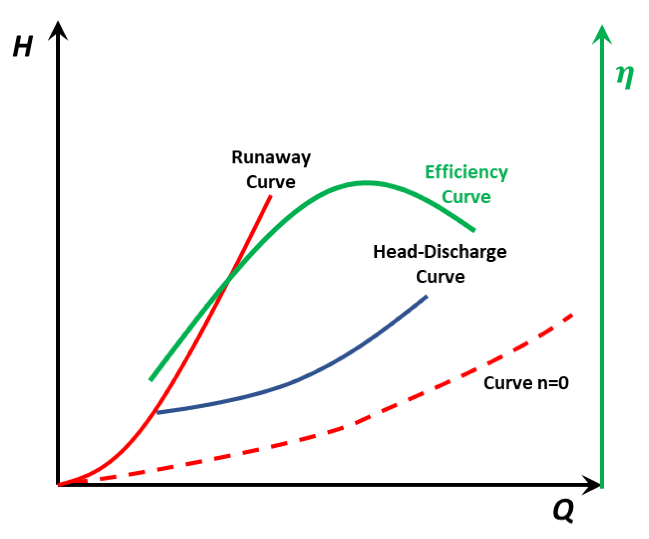
Defining empirical expressions which enable to define the head-discharge curve and efficiency curve, as well as the runaway curve, as a function of the discharge.

Both steps were studied for different researches, which will be described in the follow sections. However, this manuscript presents a new approach of these equations using a big number of experimental data (particularly, 181 machines). The use of such wide experimental information improves the prediction and reducing the error in the energy analysis.

2.2. Coefficient Proposal to Estimate the Operation Point of PAT Using Pump Manufacture

The prediction of the BEP in turbine mode based on that in the pump mode of the operation was studied by different researchers (

Table 1. Proposed empirical expressions to predict the $\beta$ coefficients

Autor	${\mathit{\beta }}_{\mathit{Q}}$	${\mathit{\beta }}_{\mathit{H}}$	${\mathit{\beta }}_{\mathit{\eta }}$
Stepanoff [19]	$\frac{1}{\sqrt{{\eta }_{p,BEP}}}$	$\frac{1}{{\eta }_{p,BEP}}$	1
Mc. Claskey [20]	$\frac{1}{{\eta }_{p,BEP}}$	$\frac{1}{{\eta }_{p,BEP}}$	1
Alatorre-Frenk [21]	$\frac{0.85{\eta }_{p,BEP}^5+0.385}{2{\eta }_{p,BEP}^{9.5}+0.205}$	$\frac{1}{0.85{\eta }_{p,BEP}^5+0.385}$	$1-\frac{0.03}{{\eta }_{p,BEP}}$
Sharma-Williams [22]	$\frac{1}{{\eta }_{p,BEP}^{0.8}}$	$\frac{1}{{\eta }_{p,BEP}^{1.2}}$	1
MICI [23]	0.9–1.0	1.56–1.78	0.75–0.80
Yang et al. [24]	$\frac{1.2}{{\eta }_{p,BEP}^{0.55}}$	$\frac{1.2}{{\eta }_{p,BEP}^{1.1}}$	-
Hancock [25]	$\frac{1}{{\eta }_{p,BEP}}$	$\frac{1}{{\eta }_{p,BEP}}$	-
Schmiedl [26]	$-1.5+\frac{2.4}{{\eta }_{p,BEP}^2}$	$-1.4+\frac{2.5}{{\eta }_{p,BEP}}$	-
Mijailov [27]	$-$0.078$n_{sp}$$+$ 3.292	$-$0.078$n_{sp}$$+$ 3.112	$-$0.0014$n_{sp}$$+$ 0.96
Audisio [28]	1.21${\eta }_{p,BEP}^{-0.25}$	1.21${\eta }_{p,BEP}^{-0.8}{\left[1+{(0.6+\ln n_{sp})}^2\right]}^{0.3}$	0.95${\eta }_{p,BEP}^{0.7}{\left[1+{(0.5+\ln n_{sp})}^2\right]}^{-0.25}$
Carvalho [29]	5·10−5$n_{sp}^2-0.0114n_{sp}^{}+1.2246$	$-$2·10−5$n_{sp}^2+0.0214n_{sp}^{}+0.7688$	-
Nautiyal [30]	30.303[(${\eta }_{p,BEP}-$ 0.212)/ln($n_{sp}$)]$-$3.424	41.667[(${\eta }_{p,BEP}-$0.212)/ln($n_{sp}$)]$-$5.042	-
Barbarelli [31]	$0.00029n_{sp}^2-0.02771 n_{sp}+2.01648$	$-3 {10}^{-5}{n}_{sp}^3+4.4 {10}^{-3}{n}_{sp}^2-0.20882 n_{sp}+4.64293$
Grover [32]	2.379 − 0.0264$n_{st}$	2.693 − 0.0229$n_{st}$	-
Hergt [33]	$1.3-\frac{1.6}{n_{st}-5}$	$1.3-\frac{6}{n_{st}-3}$	-

). These studies have resulted in proposals of different empirical methods, which predict the BEP location of a PAT with respect to its known BEP as a pump. The majority of these methods consider the specific speed of the machine ($n_s)$.

The prediction is always burdened with some uncertainty, because the change of number of blades in the impeller or the design of the machine (e.g., volute and guideline crown) cause variations in head losses and, therefore, the operation point is different [18]. However, if this uncertainty could be avoided, these methods could be a good tool to choose a pump, which will work as a turbine. The different methods relate the operation point as a turbine with the operation point as a pump according to the following:

$$Q_{t,BEP}={\beta }_Q{Q}_{p,BEP}$$

(5)

$$H_{t,BEP}={\beta }_H{H}_{p,BEP}$$

(6)

$${\eta }_{t,BEP}={\beta }_{\eta }{\eta }_{p,BEP}$$

(7)

where ${\beta }_Q$, ${\beta }_H$ and ${\beta }_{\eta }$ are the coefficients which define the ratios $\frac{Q_{t,BEP}}{Q_{p,BEP}}$, $\frac{H_{t,BEP}}{H_{p,BEP}}$ and $\frac{{\eta }_{t,BEP}}{{\eta }_{p,BEP}}$, respectively; ${\eta }_{t,BEP}$ is the best efficiency operating in the turbine mode and ${\eta }_{p,BEP}$ is the best efficiency operating in the pump mode.

The proposal of the coefficients based on a higher number of experimental data is not enough to suppose the proposed coefficients will be better than those in Table 1. Besides, according to [15], the visual comparison between predicted values (i.e., $Q_{p,BEP}$ and $H_{p,BEP}$) does not show if the prediction is good, considering the high number of experimental data. To improve the error measurement of the prediction, the authors determined different error indexes to compare the new proposal with other methods which had already been published. The evaluation of the goodness of the proposal is focused on four parameters. The used parameters were the root mean square e (RMSE), mean absolute deviation (MAD), the mean relative deviation (MRD) and BIAS:

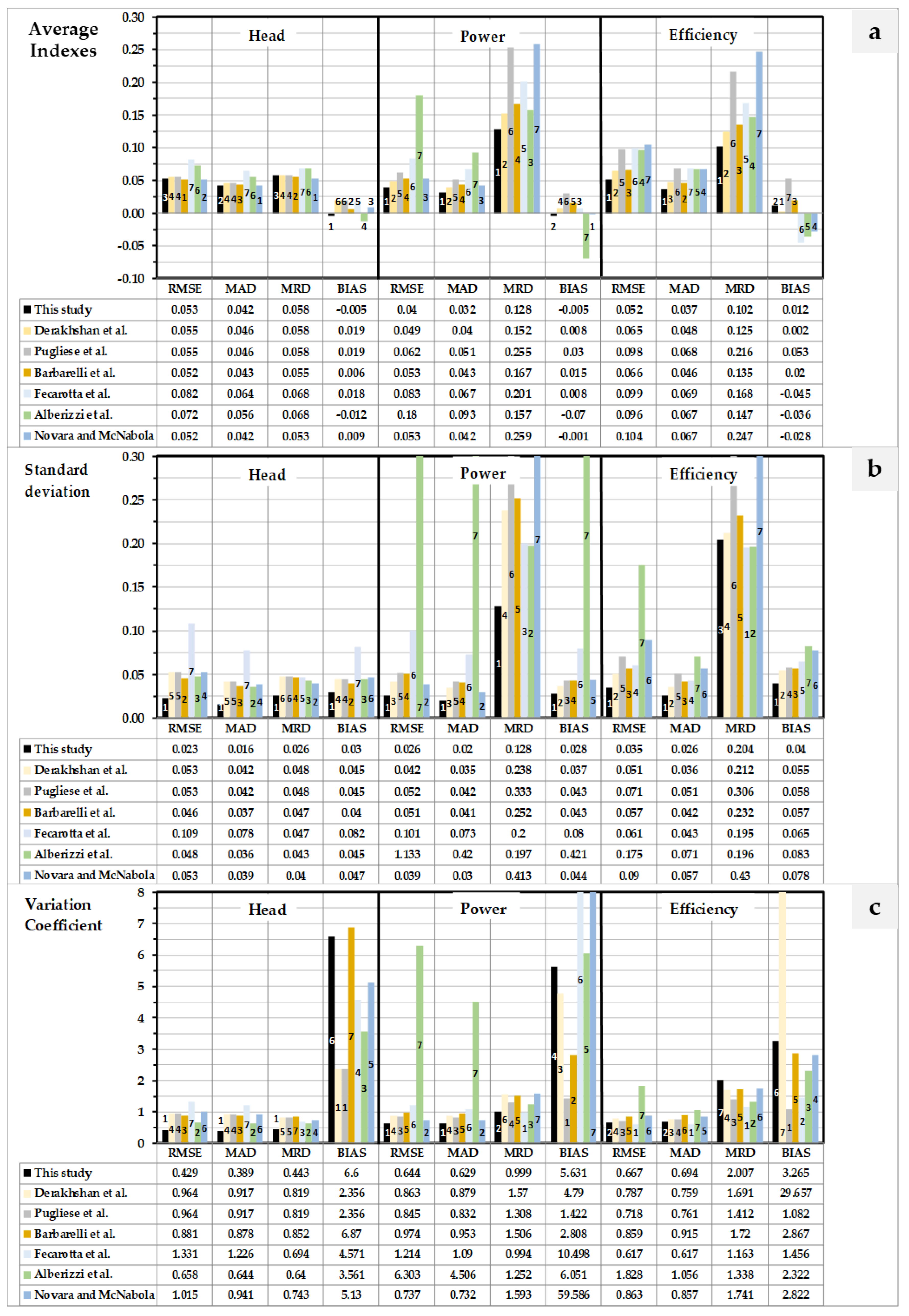
• Determination of the RMSE. This error index is a standard way to measure the error of a model in predicting quantitative data. If the RMSE is zero, this value indicates a perfect fit. Formally, it is defined as follows:

  $$RMSE=\sqrt{\frac{{{\displaystyle \sum }}_{i=1}^x{\left[O_i-P_i\right]}^2}{x}}$$

  (8)

  where $O_i$ are the estimated values, $P_i$ the experimental values and x the number of observations.
• Determination of the MAD. This index measures the average magnitude of the errors in a set of predictions without considering their direction. It is the average over the test sample of the absolute differences between prediction and actual observation where all individual differences have equal weight. If the MAD is zero, this value indicates a perfect fit. Formally, it is defined as follows:

  $$MAD={\displaystyle \sum }_1^x\frac{1}{x}\left|O_i-P_i\right|$$

  (9)
• Determination of the MRD. This index considers the weight of the error to the variable value. If the MRD is zero, this value indicates a perfect fit. Formally, it is defined as follows:

  $$MRD={\displaystyle \sum }_1^x\frac{\left|O_i-P_i\right|/P_i}{x}$$

  (10)
• Determination of the bias (BIAS). In this case, the index measures the tendency of the prediction in the variable (Q, H or efficiency), determining if the predicted values are smaller or larger than the experimental values. If the BIAS value is negative, it indicates that the method overestimates the variable, while, if the BIAS value is positive, it indicates that the variable is underestimated. This index is defined by the equation [34]:

  $$BIAS =\frac{{{\displaystyle \sum }}_{i=1}^N{\left[O_i-P_i\right]}^{}}{x}$$

  (11)

Finally, it is necessary to check the acceptability of the prediction of the turbine efficiency. It is possible using the derivation of the criterion proposed by [15], who used an ellipse to measure the difference between the predicted and the real BEP position. Figure 3 shows the characterization of the proposed ellipse. $\Delta a$ is the proportional difference parallel to the major axis of the ellipse and $\Delta b$ to the minor axis of the ellipse. The prediction is acceptable if $C\le 1$ [15]. The major and minor axis of the ellipse are defined according to ±30% and ±10% for both head and flow, respectively. Therefore, the ellipse is defined by the following equation:

$$C^2={\left(\frac{\frac{1}{2}\left(\Delta q+\Delta h\right)}{0.3}\right)}^2+{\left(\frac{\frac{1}{2}\sqrt{\Delta q^2+\Delta h^2-2\Delta q\Delta h})}{0.1}\right)}^2$$

(12)

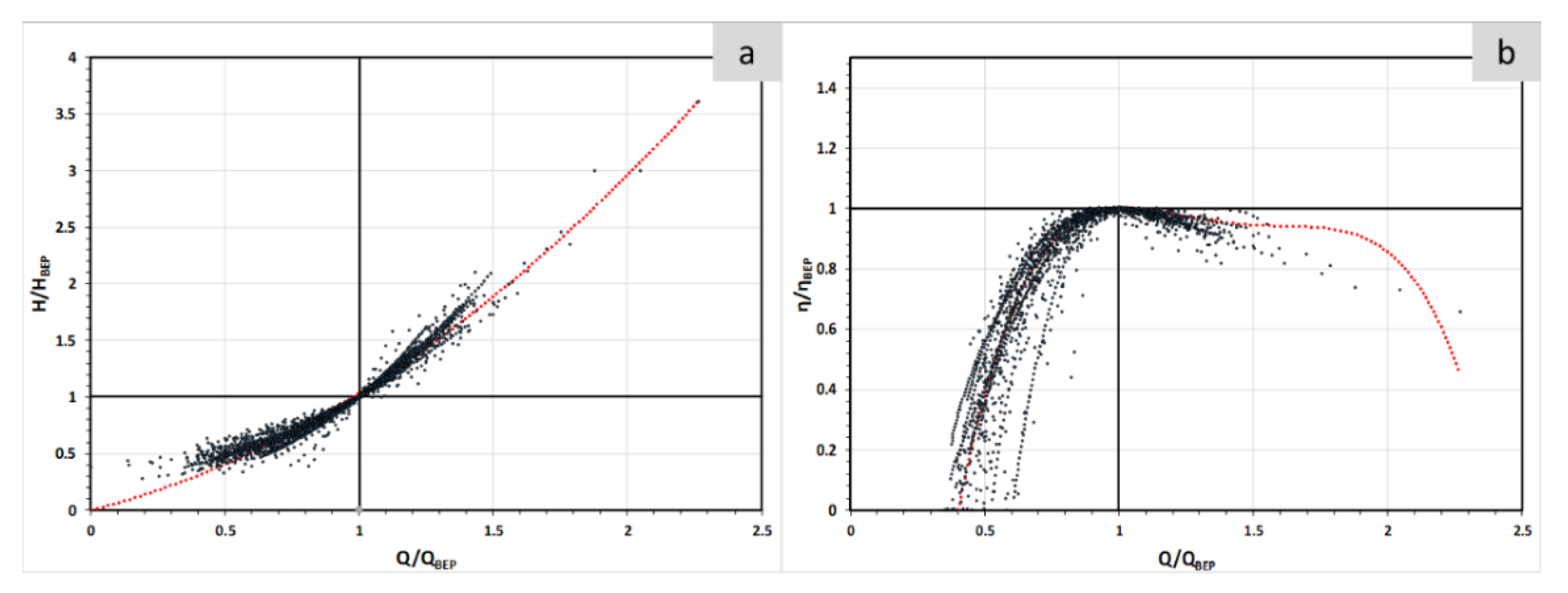
2.3. Estimation of the Head-Discharge and Efficiency Curves Considering $n_{st}$

The estimation of the BEP of the machine working as the turbine and/or the selection of the necessary pump as a function of the discharge and available head is important. However, the flow varies in a pipe or consumption node in a water network. Therefore, the estimation of the head-discharge and efficiency curves are crucial to develop energy analyses and simulations with recovery systems. Usually, the development of these curves can be developed using nondimensional numbers, particularly discharge ($\phi$) and head ($\psi$) coefficients [16].

$$\phi =\frac{Q_t}{n{D}^3}$$

(13)

$$\psi =\frac{g{H}_t}{n^2{D}^2}$$

(14)

$$\pi =\frac{P_t}{\rho n^3{D}^5}=\phi \psi {\eta }_t$$

(15)

where D is the impeller diameter in m, g is the gravity constant in m/s², $P_t$ is the shaft power in the PAT, ${\eta }_t$ is the efficiency of the PAT and n is the rotational speed in rps.

Different authors proposed empirical expressions using different numbers of experimental data, and therefore, they got different accuracy degrees in their proposals [12,31,35,36]. The expression considers the ratios $H_t/H_{t,BEP}$, $Q_t/Q_{t,BEP}$ and $P_t/P_{t,BEP}$.

Table 2. Proposed empirical expressions to predict the $\frac{H_t}{H_{t,BEP}}$ and $\frac{P_t}{P_{t,BEP}}$ as a function of $\frac{Q_t}{Q_{t,BEP}}$.

Author	Variable	Expression	Range ${\mathit{n}}_{\mathit{s}\mathit{t}}$ (Experimental Data)	Reference
Derakhshan and Nourbakhsh	$\frac{H_t}{H_{t,BEP}}$	$1.0283{\left(\frac{Q_t}{Q_{t,BEP}}\right)}^2-0.5468\frac{Q_t}{Q_{t,BEP}}+0.5314$	<60 (4)	[37]
	$\frac{P_t}{P_{t,BEP}}$	$-0.3092{\left(\frac{Q_t}{Q_{t,BEP}}\right)}^3$ + $2.1472{\left(\frac{Q_t}{Q_{t,BEP}}\right)}^2-0.8865\frac{Q_t}{Q_{t,BEP}}+0.0452$	<60 (4)	[37]
Plugiese et al.	$\frac{H_t}{H_{t,BEP}}$	They use Derakhshan’s equation.	<60 (4)	[38]
	$\frac{P_t}{P_{t,BEP}}$	$4·{10}^{-3}{\left(\frac{Q_t}{Q_{t,BEP}}\right)}^3$ + $1.386{\left(\frac{Q_t}{Q_{t,BEP}}\right)}^2-0.390\frac{Q_t}{Q_{t,BEP}}$	<45 (2)	[38]
Barbarelli et al.	$\frac{H_t}{H_{t,BEP}}$	$0.922{\left(\frac{Q_t}{Q_{t,BEP}}\right)}^2-0.406\frac{Q_t}{Q_{t,BEP}}+0.483$	<55 (12)	[31]
	$\frac{P_t}{P_{t,BEP}}$	$0.040{\left(\frac{Q_t}{Q_{t,BEP}}\right)}^3$ + 1.185${\left(\frac{Q_t}{Q_{t,BEP}}\right)}^2-0.043\frac{Q_t}{Q_{t,BEP}}-0.183$	<55 (12)	[31]
Fecarotta et al.	$\frac{H_t}{H_{t,BEP}}$	$1.61{\left(\frac{Q_t}{Q_{t,BEP}}\right)}^2-1.41\frac{Q_t}{Q_{t,BEP}}+0.805$	120–165 (4)	[13]
	$\frac{P_t}{P_{t,BEP}}$	1.85${\left(\frac{Q_t}{Q_{t,BEP}}\right)}^2-0.858\frac{Q_t}{Q_{t,BEP}}+0.00567$	120–165 (4)	[13]
Alberizzi et al.	$\frac{H_t}{H_{t,BEP}}$	$0.2394{\left(\frac{Q_t}{Q_{t,BEP}}\right)}^2+0.769\frac{Q_t}{Q_{t,BEP}}$	3 (1)	[39]
	$\frac{{\eta }_t}{{\eta }_{t,BEP}}$	−1.9778${\left(\frac{Q_t}{Q_{t,BEP}}\right)}^6+9.0636{\left(\frac{Q_t}{Q_{t,BEP}}\right)}^5-13.148{\left(\frac{Q_t}{Q_{t,BEP}}\right)}^4+3.8527{\left(\frac{Q_t}{Q_{t,BEP}}\right)}^3+4.5614{\left(\frac{Q_t}{Q_{t,BEP}}\right)}^2-1.3769\frac{Q_t}{Q_{t,BEP}}$	3 (1)	[39]
Novara and McNabola	$\frac{H_t}{H_{t,BEP}}$	$1.16{\left(\frac{Q_t}{Q_{t,BEP}}\right)}^2+\left(0.0099n_{st}-1.0627\right)\frac{Q_t}{Q_{t,BEP}}+\left(0.9027-0.0099n_{st}\right)$	<100 (113)	[12]
	$\frac{P_t}{P_{t,BEP}}$	$1.248{\left(\frac{Q_t}{Q_{t,BEP}}\right)}^2+\left(0.0108n_{st}-0.2717\right)\frac{Q_t}{Q_{t,BEP}}+\left(0.0237-0.0108n_{st}\right)$	<100 (113)	[12]

summarizes different proposed equations.

This research proposes three new equations: ($\frac{H_t}{H_{t,BEP}}=f\left(\frac{Q_t}{Q_{t,BEP}}\right),\frac{P_t}{P_{t,BEP}}=f\left(\frac{Q_t}{Q_{t,BEP}}\right)\mathrm{and}\frac{{\eta }_t}{{\eta }_{t,BEP}}=f\left(\frac{Q_t}{Q_{t,BEP}}\right)$) using a great number of PATs and leading to low errors in the prediction of the characteristic curves and efficiency curves.

Finally, two proposals were done in order to predict the runaway curve, as well as the zero-speed curve, of the machine. These curves are crucial to establishing the regulation of the machines, since the runaway curve establishes the minimum operation flow of the PAT characteristic curve.

$$H_{Runaway}=k_{Runaway}{Q}_t^2$$

(16)

$$H_{zero-speed}=k_{zero-speed}{Q}_t^2$$

(17)

where $H_{Runaway}$ is the head in m w.c. at which the machine is run without load, $k_{Runaway}$ is the coefficient proposed in this manuscript to define the polynomial of the runaway curve, $H_{zero-speed}$ is the head in m w.c. as above while the machine is in standstill (zero rotation speed) and $k_{zero-speed}$ is the coefficient proposed in this manuscript to define the polynomials of the zero-speed curve.

The analysis of the deviation between proposed curves and the experimental curves will be carried out using the average values of RMSE, MAD, MRD and BIAS, which were described in previous section. Besides, the standard deviation and variation coefficients were calculated to improve the discussion of the results.

2.4. Materials

The present manuscript used the results of 181 different PATs (Figure 4), which were published for different researches. The number of PAT curves was increased by 60% (compared to the 113 PATs used by [11]). The pumps included into the analysis are listed in Table S1 to this manuscript. The data were used according to 163 data to define the empirical method to predict the flow and head ratio when the machine is used in turbine mode. Eleven data were used to define the first prediction equation of the runaway curve and zero-speed curve (‘n = 0’ curve) from [40]. Besides, the used databases enabled to process 103 experimental curves in the prediction of the head-discharge curves (Figure 5).

Using the depicted database, 1952 Q,H points were obtained, as well as 1976 $Q,\eta$ points, developing the power calculus by interpolating and normalizing each digitalized curve to get the points of H and $\eta$ for the same value of flow. Figure 4 shows the map of used PATs in the experimental data. This figure enables water managers to estimate discharge and efficiency according to $n_{sp}$ and head. Figure 5 allows the designers to estimate the head number and efficiency using the specific speed of the machine in order to know the head-discharge curve when the PAT is chosen.

3. Results

3.1. Comparison between the Proposed and Others Methods to Predict the Flow and Head in Pump Mode. First Approach to Predict Runaway Curve

The analysis of the experimental data described in the materials section enabled to define different $\beta$ coefficients, as well as to establish the correlation between $n_{sp}$ and $n_{st}$. The derived relationships are listed in

Table 3. Proposed empirical relationship to define the best efficiency point of the machine as a function of the specific speed.

Coefficient	Empirical Equation	R2	Experimental Data
$n_{st}$	$0.844564\times n_{sp}$	99.34	163
${\beta }_Q$	${\beta }_Q=\frac{1}{0.825861\times \sqrt{{\eta }_{p,BEP}}}$	98.85	150
${\beta }_H$	${\beta }_H=\frac{1.2337}{{\eta }_{p,BEP}}$	97.59	150
$n_{sp}$	$1.17619\times n_{st}$	99.34	163
${\beta }_Q$	$\frac{1}{0.210551\times \ln \left(n_{st}\right)}$	97.15	157
${\beta }_H$	$\frac{1}{0.186314\times \ln \left(n_{st}\right)}$	96.39	153
$k_{Runaway}$	$k_{Runaway}={\left(\frac{6.83008}{n_{st}}\right)}^2$	96.39	11
$k_{zero-speed}$	$k_{zero-speed}={\left(\frac{4.36583}{n_{st}}\right)}^2$	90.92	11

. The expressions are defined as functions $n_{sp}$ or $n_{st}$. It is because the water manager could be interested in one or other specific speed depending on the need (i.e., if the water manager needs to choose a pump because $Q_T$ and $H_T$ are known, the $n_{st}$ number must be used. If the water manger wants to know the operation point in turbine mode, the $n_{sp}$ number will be used.). All analyses were applied at the BEP when the BEP was studied. Otherwise, the entire set was considered when the analysis studied the characteristic curves.

Table 3 also shows the estimated value to predict the runaway curve, as well as the zero-speed curve, when the axis of the machine is fixed (‘n = 0’). This proposal is a novelty, since the runaway curve was only estimated by [40] using a single couple of data.

The proposed equations were compared with the rest of enumerated methods in Table 1, determining the error indexes of RMSE, MAD, MRD and BIAS, as well as the consideration of the acceptability inside of the ellipse ($C\le 1)$.

Table 4. Error indexes depending on applied method to predict BEP in turbine mode.

Method	Flow (Q)				Head (H)				Efficiency				Q,H
	RMSE	MAD	MRD	BIAS	RMSE	MAD	MRD	BIAS	RMSE	MAD	MRD	BIAS	% data C<1
This study	0.181 (1)	0.135 (1)	0.091 (1)	−0.037 (2)	0.294 (2)	0.211 (2)	0.129 (2)	−0.02 (3)	0.078 (1)	0.059 (1)	0.068 (1)	−0.004 (1)	79.20 (1)
Yang	0.192 (2)	0.138 (2)	0.092 (2)	−0.036 (1)	0.288 (1)	0.209 (1)	0.129 (1)	−0.011 (2)	−	−	−	−	78.81 (2)
Mc Claskey	0.205 (3)	0.16 (3)	0.107 (3)	−0.073 (3)	0.466 (7)	0.381 (7)	0.206 (7)	−0.343 (8)	0.114 (4)	0.088 (4)	0.106 (4)	0.08 (4)	62.42 (5)
Sharma-Williams	0.238 (4)	0.195 (5)	0.128 (5)	−0.163 (5)	0.379 (5)	0.303 (6)	0.169 (5)	−0.245 (7)	0.114 (4)	0.088 (4)	0.106 (4)	0.08 (4)	71.83 (4)
Audisio	0.252 (5)	0.192 (4)	0.122 (4)	−0.148 (4)	0.359 (4)	0.257 (4)	0.145 (4)	−0.117 (4)	0.192 (7)	0.161 (7)	0.162 (7)	−0.16 (7)	74.49 (3)
Alatorre-Frenk	0.321 (6)	0.259 (6)	0.185 (6)	0.184 (7)	0.321 (3)	0.223 (3)	0.135 (3)	−0.009 (1)	0.089 (2)	0.064 (2)	0.075 (2)	0.039 (3)	60.93 (6)
Stepanoff	0.339 (7)	0.29 (7)	0.187 (7)	−0.285 (8)	0.466 (7)	0.381 (7)	0.206 (7)	−0.343 (8)	0.114 (4)	0.09 (4)	0.106 (4)	0.08 (4)	46.98 (8)
Carvalo	0.6 (8)	0.558 (9)	0.371 (9)	−0.558 (10)	0.875 (9)	0.62 (9)	0.352 (9)	−0.195 (6)	−	−	−	−	9.27 (11)
Barbarelli	0.878 (9)	0.312 (8)	0.244 (8)	0.177 (6)	10.717 (12)	2.087 (12)	1.668 (12)	−1.798 (12)	−	−	−	−	60.27 (7)
Nautiyal	1.304 (10)	0.784 (10)	0.504 (10)	−0.332 (9)	1.858 (10)	1.166 (10)	0.655 (10)	−0.505 (10)	−	−	−	−	21.85 (9)
Schimiedl	2.504 (11)	1.783 (12)	1.153 (12)	1.783 (12)	0.395 (6)	0.282 (5)	0.173 (6)	0.194 (5)	−	−	−	−	3.35 (12)
Mijailov	2.523 (12)	1.362 (11)	1.038 (11)	−1.143 (11)	2.725 (11)	1.64 (11)	1.087 (11)	−1.588 (11)	0.091 (3)	0.068 (3)	0.076 (3)	−0.02 (2)	13.91 (10)

(x) indicates the classified order of the method considering the rest of the methods.

shows the error values for each method considering all databases (181 different machines). The error was evaluated for discharge, head and efficiency.

If Table 4 is observed, the proposed method provides the best error indexes for flow and efficiency, while it was second if the head error was considered. However, the head error estimations according to Yang’s methodology and that proposed in this manuscript are close to each other, and the difference is lower than 2%, except for MRD and BIAS, which show discrepancy of around 5% and 7%, respectively.

If the percentage of data inside of the uncertainty ellipse is considered ($C\le 1)$, the proposed method reached near 80% of the pair of points inside of the ellipse. Therefore, the proposal was much better than the rest of methods. Considering Table 4, the use of the proposal method will improve the BEP prediction when the water manager wants to choose a pump to work as turbine. Yang’s Method got similar results, being higher the error indexes except for head values. This method had 78% of data inside of the ellipse. If the order is observed, considering the C value, Sharma’s and Audisio’s methods were located on third and fourth position.

Finally,

Table 5. Error indexes depending on applied method to predict BEP in pump mode. MAD: mean absolute deviation, MRD: mean relative deviation, BIAS: bias and RMSE: root mean square error.

Method	Flow (Q)				Head (H)				Efficiency				Q,H
	RMSE	MAD	MRD	BIAS	RMSE	MAD	MRD	BIAS	RMSE	MAD	MRD	BIAS	% C<1
This study	0.291 (1)	0.206 (1)	0.144 (1)	0.068 (1)	0.357 (1)	0.264 (1)	0.165 (1)	−0.006 (1)	0.072 (1)	0.054 (1)	0.063 (1)	−0.003 (1)	69.54 (1)
Hergt	1.602 (2)	0.462 (2)	0.272 (2)	−0.433 (2)	1.157 (3)	0.835 (3)	0.419 (3)	−0.82 (3)	-		-	-	31.79 (2)
Grover	1.915 (3)	1.173 (3)	0.882 (3)	−1.125 (3)	0.624 (2)	0.487 (2)	0.331 (2)	0.225 (2)	-	-	-	-	7.28 (3)

(x) indicates the classified order of the method considering the rest of methods.

shows the results of the error indexes, which were obtained when the proposed method was used to predict the curves from turbine to pump. If the method is compared to the methods of Hergb and Grover, the error values were always lower.

The percentage of the data inside of the ellipse was near 70%, while the rest of methods presented 32% and 7% error percentages (Table 5). When the order was established considering the minor error and higher % of data inside of the ellipse, the proposed method in this research was the best, while the Hergt’s and Grover’s methods were second and third, respectively.

3.2. Estimation of the Operation and Effciency Curve

The derived expressions to predict the characteristic, power and efficiency curves are defined in the following equations using a regression by the least square method:

$$\frac{H_t}{H_{t,BEP}}=0.406{\left(\frac{Q_t}{Q_{t,BEP}}\right)}^2+0.621\left(\frac{Q_t}{Q_{t,BEP}}\right) \left(R^2=99.41\%\right)$$

(18)

$$\frac{P_t}{P_{t,BEP}}=-0.333{\left(\frac{Q_t}{Q_{t,BEP}}\right)}^3+2.19{\left(\frac{Q_t}{Q_{t,BEP}}\right)}^2-0.863\left(\frac{Q_t}{Q_{t,BEP}}\right) \left(R^2=99.57\%\right)$$

(19)

$$\begin{array}{c}\frac{{\eta }_t}{{\eta }_{t,BEP}}=-1.219{\left(\frac{Q_t}{Q_{t,BEP}}\right)}^4+6.95{\left(\frac{Q_t}{Q_{t,BEP}}\right)}^3-14.578{\left(\frac{Q_t}{Q_{t,BEP}}\right)}^2+13.231\left(\frac{Q_t}{Q_{t,BEP}}\right)-\\ 3.383\left(R^2=99.45\%\right)\mathrm{for}\mathrm{values}\frac{Q_t}{Q_{t,BEP}}\ge 0.4\end{array}$$

(20)

Figure 6 shows the experimental data approximation according to equations proposed by the authors. The $H_t$ values can be considered acceptable for any interval of $\frac{Q_t}{Q_{t,BEP}}$. This study considered experimental data between 0.1 and 2.3 being 93% of the values between 0.4 and 1.6. In all cases, the experimental data show a high decrease of the efficiency for values below 0.7$\frac{Q_t}{Q_{t,BEP}}$. This value should be considered in order to establish the limits to operate with the machine considering the invariable rotational speed. The analysis of the errors was similar to the prediction of the BEP of the machine operating as turbine. In this case, the average of the RMSE, MAD, MRD and BIAS were determined for the experimental curves for both heads, power and efficiency. These error indexes were determined using a new proposal, as well as the published methods, which were enumerated in Table 2.

Besides, the standard deviation and the variation coefficient (i.e., ratio between standard deviation and average) was determined for each parameter and method in order to compare between them, because the indexes were near between them. These results are shown in

Table 6. Error indexes for runaway and zero-speed curves.

Curve	RMSE	MAD	MRD	BIAS
Runaway	0.139	0.0946	0.0529	−0.0135
Zero-speed	0.1289	0.0855	0.1036	−0.0183

. If the head error indexes are observed, the new proposal showed values close to Barbarelli and Novara, particularly around 0.05. When the indexes for runaway and zero-speed curves were determined, the results were according to Table 6. The validated range of specific speeds to use the runaway and zero-speed curves is between 5.09 and 52.6 (m, kw).

Figure 7 shows that the prediction of the characteristic curves contains an implicit uncertainty. Therefore, the use of these curves should be thorough when the results want to extrapolate to the energy analysis, being necessary for the real experimental curve to define exactly the feasibility indexes of the installation. However, the use of these equations, which are supported in a higher experimental database, can give water managers an advantage to develop simulations and analyses less uncertainly. If Figure 7 is analyzed, the classified order can be observed considering the different indexes.

When the power and efficiency curves were compared, the new proposal showed lower error and deviation indexes (RMSE, MAD and MRD) than the rest of methods. Besides, if the standard deviation is considered, the new proposal presented the best value, reaching the first method in the established classification. An identical position was reached when the variation coefficient was determined, except for RMSE, in which the proposed method was second after Fecarotta’s methods. The proposed method had the worst order when the variation coefficients of MRD and BIAS were considered, particularly in the determination of the efficiency. However, the main index (RMSE) reached values which were lower than obtained values using the rest of methods, except the RMSE head error, where the determined value was third. Particularly, when the order in head error was established, the Derakhshan’s and Plugiese’s methods had the same order, since Plugiese used the same head equation as Derakhshan.

4. Conclusions

The manuscript did a deep review of the different methods to predict the BEP of a PAT when the BEP of the pump is known. Besides, the research established the higher database of experimental curves of PATs, which was used to propose a new empirical method to predict the BEP of a PAT. This new method was compared with the rest of published methods (particularly, eleven). The comparison arose that the proposed method had the minor error indexes and the high percentage of points in the error ellipse. Therefore, if the BEP wants to be predicted, the new proposal shows less error than other empirical methods. Similar results were obtained when the proposal was compared with the methods which are used to predict the BEP of a pump when the specific speed is known.

The research also proposed new empirical equations in order to define the characteristic curves (head, efficiency and power) of the machine as a function of the discharge and considering the BEP. This new proposal was also compared with other published expressions (particularly, five). The comparison showed the new proposal improved the results, reducing the error indexes and, therefore, improving the prediction. Besides, as a novelty, the research also proposed empirical expressions to predict the runaway and zero-speed curves in a machine. These curves are crucial to define the flow range of the machine and, therefore, the establishment of the regulation limits.

The contribution of this research improves the prediction of the BEP characteristics curves of the machine, showing good indexes to measure the uncertainty compared with the rest of the methods. This comparison showed the proposed method was the best in the majority of the cases.

The present research is focused on proposing new equations in order to predict the BEP operating as a turbine, as well as the characteristic curves as a function of discharge. The manuscript compared the errors and deviations between the proposed model and the experimental data in order to propose an analytical model which reduces the uncertainty of the water managers when they will develop energy analyses using PATs. The knowledge of expressions which can be used to propose PATs is crucial to improving the simulation in energy analyses of water systems. Their use will improve the uncertainty to estimate the energy recovery and, therefore, the sustainability improvements in water systems.

References

1. Coelho, B.; Andrade-Campos, A. Efficiency achievement in water supply systems—A review. Renew. Sustain. Energy Rev. 2014, 30, 59–84. [Google Scholar] [CrossRef]
2. Ramos, H.; Borgå, Å. Pumps as turbines: An unconventional solution to energy production. Urban Water 1999, 1, 261–263. [Google Scholar] [CrossRef]
3. Goonetilleke, A.; Vithanage, M. Water Resources Management: Innovation and Challenges in a Changing World. Water 2017, 9, 281. [Google Scholar] [CrossRef]
4. Carravetta, A.; Fecarotta, O.; Del Giudice, G.; Ramos, H. Energy Recovery in Water Systems by PATs: A Comparisons among the Different Installation Schemes. Procedia Eng. 2014, 70, 275–284. [Google Scholar] [CrossRef] [Green Version]
5. Carravetta, A.; Del Giudice, G.; Fecarotta, O.; Ramos, H.M. PAT Design Strategy for Energy Recovery in Water Distribution Networks by Electrical Regulation. Energies 2013, 6, 411–424. [Google Scholar] [CrossRef] [Green Version]
6. Pérez-Sánchez, M.; Sánchez-Romero, F.J.; Ramos, H.M.; López-Jiménez, P.A. Energy Recovery in Existing Water Networks: Towards Greater Sustainability. Water 2017, 9, 97. [Google Scholar] [CrossRef] [Green Version]
7. Stefanizzi, M.; Capurso, T.; Balacco, G.; Binetti, M.; Torresi, M.; Camporeale, S.M. Pump as Turbine for Throttling Energy Recovery in Water Distribution Networks; AIP Publishing LLC: Melville, NY, USA, 2019; Volume 2191, p. 020142. [Google Scholar]
8. Muhammetoglu, A.; Nursen, C.; Karadirek, I.E.; Muhammetoglu, H. Evaluation of performance and environmental benefits of a full-scale pump as turbine system in Antalya water distribution network. Water Sci. Technol. Water Supply 2018, 18, 130–141. [Google Scholar] [CrossRef]
9. Stefanizzi, M.; Capurso, T.; Balacco, G.; Torresi, M.; Binetti, M.; Piccinni, A.F.; Camporeale, S.M. Preliminary assessment of a pump used as turbine in a water distribution network for the recovery of throttling energy. In Proceedings of the 13th European Conference on Turbomachinery Fluid dynamics & Thermodynamics, European Turbomachinery Society, Lausanne, Switzerland, 8–12 April 2019. [Google Scholar]
10. Pérez-Sánchez, M.; Sánchez-Romero, F.J.; Ramos, H.M.; López-Jiménez, P.A. Optimization Strategy for Improving the Energy Efficiency of Irrigation Systems by Micro Hydropower: Practical Application. Water 2017, 9, 799. [Google Scholar] [CrossRef] [Green Version]
11. Novara, D.; McNabola, A. The Development of a Decision Support Software for the Design of Micro-Hydropower Schemes Utilizing a Pump as Turbine. Proceedings 2018, 2, 678. [Google Scholar] [CrossRef] [Green Version]
12. Novara, D.; McNabola, A. A model for the extrapolation of the characteristic curves of Pumps as Turbines from a datum Best Efficiency Point. Energy Convers. Manag. 2018, 174, 1–7. [Google Scholar] [CrossRef]
13. Fecarotta, O.; Carravetta, A.; Ramos, H.M.; Martino, R. An improved affinity model to enhance variable operating strategy for pumps used as turbines. J. Hydraul. Res. 2016, 54, 332–341. [Google Scholar] [CrossRef]
14. Pérez-Sánchez, M.; López-Jiménez, P.A.; Ramos, H.M. Modified Affinity Laws in Hydraulic Machines towards the Best Efficiency Line. Water Resour Manag. 2018, 32, 829–844. [Google Scholar] [CrossRef] [Green Version]
15. Williams, A.A. The Turbine Performance of Centrifugal Pumps: A Comparison of Prediction Methods. Proc. Inst. Mech. Eng. Part A J. Power Energy 1994, 208, 59–66. [Google Scholar] [CrossRef]
16. Mataix, C. Turbomáquinas Hidráulicas; Universidad Pontificia Comillas: Madrid, Spain, 2009. [Google Scholar]
17. Ulanicki, B.; Kahler, J.; Coulbeck, B. Modeling the Efficiency and Power Characteristics of a Pump Group. J. Water Resour. Plan. Manag. 2008, 134, 88–93. [Google Scholar] [CrossRef]
18. Capurso, T.; Stefanizzi, M.; Pascazio, G.; Ranaldo, S.; Camporeale, S.M.; Fortunato, B.; Torresi, M. Slip Factor Correction in 1-D Performance Prediction Model for PaTs. Water 2019, 11, 565. [Google Scholar] [CrossRef] [Green Version]
19. Stepanoff, A.J. Centrifugal and Axial Flow Pumps. Theory, Design, and Application; Krieger Publishing Company: Malabar, FL, USA, 1957. [Google Scholar]
20. McClaskey, B.M.; Lundquist, J.A. Hydraulic power recovery turbine. In Mechanical Engineering; AMER Soc Mechanical Eng 345 E 47TH ST; ASME: New York, NY, USA, 1977; Volume 10017, p. 106. [Google Scholar]
21. Alatorre-Frenk, C. Cost Minimisation in Micro-Hydro Systems Using Pumps-as-Turbines. 1994. Available online: http://wrap.warwick.ac.uk/36099/ (accessed on 20 December 2019).
22. Sharma, K. Small Hydroelectric Project-Use of Centrifugal Pumps as Turbines; Kirloskar Electric Co.: Bangalore, India, 1985. [Google Scholar]
23. Krivchenko, G.I. Recomendaciones Para la Utilización de Bombas Como Turbinas (en ruso); Muraviob, O.A., Natarius, E.M., Eds.; Infoenergo: Saint Petersburg, Russia, 1990. [Google Scholar]
24. Yang, S.-S.; Derakhshan, S.; Kong, F.-Y. Theoretical, numerical and experimental prediction of pump as turbine performance. Renew. Energy 2012, 48, 507–513. [Google Scholar] [CrossRef]
25. Hancock, J.W. Centrifugal pump or water turbine. Pipe Line News 1963, 6, 25–27. [Google Scholar]
26. Schmiedl, E. Serien-Kreiselpumpen im Turbinenbetrieb; Pumpentagung: Karlsruhe, Germany, 1988. [Google Scholar]
27. Mijailov, L.P.; Feldman, B.N. Pequeña Hidroenergía (en ruso); Energoatomizdat: Moscú, Russia, 1989. [Google Scholar]
28. Audisio, O. Bombas Utilizadas Como Turbinas; Universidad nacional del Comahue: Buenos Aires, Argentina, 2009. [Google Scholar]
29. Carvalho, N. Bombas de Fluxo Operando Como Turbina. Por Que Usá-Las? Seção de Artigos Técnicos. PCH Notícias & SPH News. 2012. Available online: http://www.proceedings.scielo.br/scielo.php?script=sci_arttext&pid=MSC0000000022002000100033&lng=en&nrm=iso (accessed on 31 December 2019).
30. Nautiyal, H.; Kumar, A. Reverse running pumps analytical, experimental and computational study: A review. Renew. Sustain. Energy Rev. 2010, 14, 2059–2067. [Google Scholar] [CrossRef]
31. Barbarelli, S.; Amelio, M.; Florio, G. Experimental activity at test rig validating correlations to select pumps running as turbines in microhydro plants. Energy Convers. Manag. 2017, 149, 781–797. [Google Scholar] [CrossRef]
32. Grover, K.M. Conversion of Pumps to Turbines; GSA Inter Corp.: Katonah, NY, USA, 1980. [Google Scholar]
33. Lewinsky-Kesslitz, H.-P. Pumpen als turbinen fur kleinkraftwerke. Wasserwirtschaft 1987, 77, 531–537. [Google Scholar]
34. Moriasi, D.N.; Arnold, J.G.; Van Liew, M.W.; Bingner, R.L.; Harmel, R.D.; Veith, T.L. Model Evaluation Guidelines for Systematic Quantification of Accuracy in Watershed Simulations. Trans. Asabe 2007, 50, 885–900. [Google Scholar] [CrossRef]
35. Rossi, M.; Renzi, M. A general methodology for performance prediction of pumps-as-turbines using Artificial Neural Networks. Renew. Energy 2018, 128, 265–274. [Google Scholar] [CrossRef]
36. Rossi, M.; Nigro, A.; Renzi, M. Experimental and numerical assessment of a methodology for performance prediction of Pumps-as-Turbines (PaTs) operating in off-design conditions. Appl. Energy 2019, 248, 555–566. [Google Scholar] [CrossRef]
37. Derakhshan, S.; Nourbakhsh, A. Experimental study of characteristic curves of centrifugal pumps working as turbines in different specific speeds. Exp. Therm. Fluid Sci. 2008, 32, 800–807. [Google Scholar] [CrossRef]
38. Flórez, R.; Abella Jiménez, J. Máquinas Hidráulicas Reversibles Aplicadas a Micro Centrales Hidroeléctricas. IEEE Lat. Am. Trans. 2008, 6, 170–175. [Google Scholar]
39. Alberizzi, J.; Renzi, M.; Righetti, M.; Pisaturo, G.; Rossi, M. Speed and Pressure Controls of Pumps-as-Turbines Installed in Branch of Water-Distribution Network Subjected to Highly Variable Flow Rates. Energies 2019, 12, 4738. [Google Scholar] [CrossRef] [Green Version]
40. Gülich, J.F. Centrifugal Pumps; Springer: Berlin, Germany, 2008; Volume 2. [Google Scholar]
Figure 1. Characteristics curves in a pump working as a turbine (PAT).
Water 12 00468 g001
Figure 2. Characteristics curves in a PAT.
Water 12 00468 g002
Figure 3. Limits of the acceptable prediction.
Water 12 00468 g003
Figure 4. PATs classified according to n s p (m, kw).
Water 12 00468 g004
Figure 5. Experimental curves as a function of n s t .
Water 12 00468 g005
Figure 6. Estimation of the head and efficiency curve as a function of BEP (red line is the estimation of (a) H t H and (b) η t η t , B E P ). Red line is an equation defined by Equations (18) and (20).
Water 12 00468 g006
Figure 7. (a) Average indexes, (b) standard deviation and (c) variation coefficient in the prediction depending on the applied method. The number which is located in each bar (x) indicates the classified order of the method considering the rest of methods.
Water 12 00468 g007