A Comparative Study of Statistical Methods for Daily Streamflow Estimation at Ungauged Basins in Turkey

Abstract

In this study, a comparative evaluation of the statistical methods for daily streamflow estimation at ungauged basins is presented. The single donor station drainage area ratio (DAR) method, the multiple-donor stations drainage area ratio (MDAR) method, the inverse similarity weighted (ISW) method, and its variations with three different power parameters (1, 2, and 3) are applied to the two main subbasins of the Euphrates Basin in Turkey to estimate daily streamflow data. Each station in each basin is considered in turn as the target station where there are no streamflow data. The donor stations are selected based on the physical similarities between the donor and target stations. Then, streamflow data from the most physically similar donor station(s) is transferred to the target station using the statistical methods. In addition, the effect of data preprocessing on the estimation performance of the statistical methods is investigated. The preprocessing discussed in this study is streamflow data smoothing using the two-sided moving average (MA). Three statistical methods using the smoothed data by the MA, named as DAR-MA, MDAR-MA, and ISW-MA, are proposed. The estimation performance of the statistical methods is compared by using daily streamflow data with preprocessing and without preprocessing. The Nash–Sutcliffe efficiency (NSE), the ratio of the root mean square error (RMSE) to the standard deviation of the observed data (RSR), the percent bias (PBIAS), and the coefficient of determination (R²) are used to evaluate the performance of the statistical methods. The results show that MDAR and ISW give improved performances compared to DAR to estimate daily streamflow for 7 out of 8 target stations in the Middle Euphrates Basin and for 4 out of 7 target stations in the Upper Euphrates Basin. Higher NSE values for both MDAR and ISW are mostly obtained with the three most physically similar donor stations in the Middle Euphrates Basin and with the two most physically similar donor stations in the Upper Euphrates Basin. The best statistical method for each target station exhibits slightly greater NSE when the smoothed data by the MA is used for all target stations in the Middle Euphrates Basin and for 6 out of 7 target stations in the Upper Euphrates Basin.

1. Introduction

In recent years, several factors, such as climate change, global warming, drought, population growth, and industrialization, have led to a rapid increase in demand for water. Hence, issues related to the planning and implementation of the water budget become important. Measurements and estimates of streamflow play an important role in the stage of the planning and implementation of the water budget. Since drainage basins in many parts of the world are ungauged or poorly gauged, the International Association of Hydrological Sciences (IAHS) launched a scientific decade from 2003 to 2012 on Predictions in Ungauged Basins (PUB) [1]. It was an effort to improve streamflow estimations for ungauged basins. Streamflow estimation at ungauged and poorly gauged basins is an important issue in growing economies countries such as Turkey because there are a limited number of stations in the streamflow gauging network of Turkey and streamflow estimates are often needed at ungauged basins where water resources projects are planned. Some stations in the river basins of Turkey contain large amounts of missing data during the observation period [2,3]. This lack of adequate data creates significant problems in the water resources projects for Turkey. For these reasons, accurate measurement and analysis of streamflow data and reliable streamflow estimates are needed.

Many methods have been used to improve the reliability and the accuracy in estimations for the development of streamflow estimation methods, and the research in this area still continues. In order to estimate streamflow, several researchers have suggested the artificial intelligence methods such as artificial neural networks [4,5,6], fuzzy logic [7,8,9], genetic programming [10,11,12], and machine learning [13,14,15]. In addition, artificial intelligence methods have been coupled with the data preprocessing methods to improve streamflow estimation accuracy and reliability in recent studies in the literature [16,17,18,19]. For example, Wu and Chau [20] used data preprocessing methods such as moving average (MA) and singular spectrum analysis (SSA) in order to improve the performance of artificial neural networks (ANN). Results showed that the MA was more effective than the SSA when they were coupled with the ANN. Moreover, ANN methods coupled with the MA performed the best among all methods. On the other hand, statistical methods such as interpolation by inverse distance weighted (IDW) [21,22] and kriging [23,24], regression analysis [25,26], flow duration curves [27,28], and information transfer methods [29,30] are widely used in the estimation of streamflow. This study focuses on statistical methods for improving estimation accuracy and reliability for ungauged basins.

Regionalization is a statistical process, which aims to estimate streamflow at ungauged basins. Various regional methods have been used for regional estimation of streamflow for the different time scales (i.e., daily, monthly, or annually) at ungauged basins in the literature [31,32,33,34,35]. Streamflow estimation at ungauged basins where streamflow data are not available requires the transfer of hydrologic information available at a donor station to the target station where only morphological and meteorological characteristics are available [36]. Drainage area ratio (DAR) method is one of the oldest information transfer methods for obtaining streamflow values at the target station from the donor station. This method is straightforward to apply and is in widespread use by hydrologists because it requires no additional information other than the streamflow values at the target station and the drainage areas of the donor and target stations. The DAR method has gained acceptance in Turkey as well, and it is widely used to estimate streamflow for ungauged basins in Turkey [2,3]. In the traditional application of this method, area-normalized streamflow values are transferred from only a single donor station to the target station. In addition to the drainage area, there are some other factors that have a significant influence on the unique streamflow characteristics of a station. Because the DAR method is used with only a single donor station, systematic errors can be encountered in the estimation of a target station [32]. When more streamflow gauging stations are used to estimate streamflow for the target station, this method is referred to as the multiple-donor stations drainage area ratio (MDAR) method [2,32]. The MDAR method assumes that the streamflow estimates at the target station can be computed as the weighted average of the estimates (produced by the DAR method) of the multiple donor stations selected.

The inverse distance weighted (IDW) method is one of the most widely used interpolation methods based on the geographical distance between the donor and target stations [21,22]. This method can be considered as a variant of the DAR method. The IDW method estimates the streamflow value for the target station by taking the geographical distance between the donor station and the target station as the weight. The closer the geographical distance between the donor station and the target station is, the larger the influence on the target station will be. That is, when the distance decreases, the weight coefficient increases. The IDW method, also called an inverse distance to power, is a weighted average interpolator, and the main factor affecting the accuracy of the IDW method is the value of the power parameter. As the power parameter increases, more influence is given to the donor stations close to the target station. In the literature, the value of the power parameter is commonly chosen as 2, which is known as the inverse distance squared weighted [36]. Alternatively, the inverse similarity weighted (ISW) method [37,38], which is similar to the IDW method, can be applied on the basis of multiple donor stations. Unlike the IDW method, the ISW method uses physical similarity instead of the geographical distance between the target and the donor station. The ISW method with three different power parameters (1, 2, and 3) was used for daily streamflow estimation in this study, and area normalized streamflow values are directly transferred to a target station from multiple donor stations.

The streamflow characteristics at the ungauged basin are directly affected by the donor stations. Therefore, the selection of hydrologically similar donor stations is important for estimating streamflow values at the ungauged basin. In practical applications, the donor station is usually selected as the geographically nearest station to the ungauged basin [36,39,40]. However, the geographical distance may not always be correct for the selection of the donor stations [41,42]. In this study, the physical similarities between the donor and the target station were taken into account when selecting the appropriate donor station for the target station. Physical similarity defines which stations are most similar in terms of some physical characteristics such as drainage area, elevation, precipitation, temperature, latitude, and longitude. According to the physical similarity, donor stations were defined for each target station. This procedure is described in detail in the section “Selection of Donor Stations”.

In this study, continuous daily streamflow data were used between 1986–2009 for selected streamflow gauging stations in two subbasins of the Euphrates basin. In order to estimate daily streamflow at the ungauged basin, the single-donor station drainage area ratio (DAR) method, the multiple-donor stations drainage area ratio (MDAR) method, and the inverse similarity weighted (ISW) methods were applied. Three different power parameters (1, 2, and 3) of the ISW method were compared to determine their accuracy and suitability for estimating daily streamflow values. In addition, the daily streamflow data were smoothed with symmetric two-sided moving average (MA) filtering in order to reduce noise. The observed (original) data (without data preprocessing) or the smoothed data (with data preprocessing by the MA) were used as inputs of the statistical methods for estimating daily streamflow values at the target station. In the former case, the estimated daily streamflow values at the target station were compared to the observed (original) daily streamflow values at the target station, while in the latter case, the estimated daily streamflow values at the target station were compared to the observed-MA (smoothed) daily streamflow values at the target station. These two approaches were presented to estimate the daily streamflow values with and without MA. It is believed that the results will help decision makers choose the best one for their objectives. In summary, the major objectives of this study can be listed as follows: 1) to test applicability of the statistical methods to two subbasins of the Euphrates basin in Turkey, 2) to evaluate the success of physical similarity approaches in selecting donor stations in this basin, and 3) to investigate the effect of the statistical methods coupled with the data preprocessing method of moving average (MA) on the accuracy of streamflow estimation.

2. Study Area and Data

2.1. Study Area

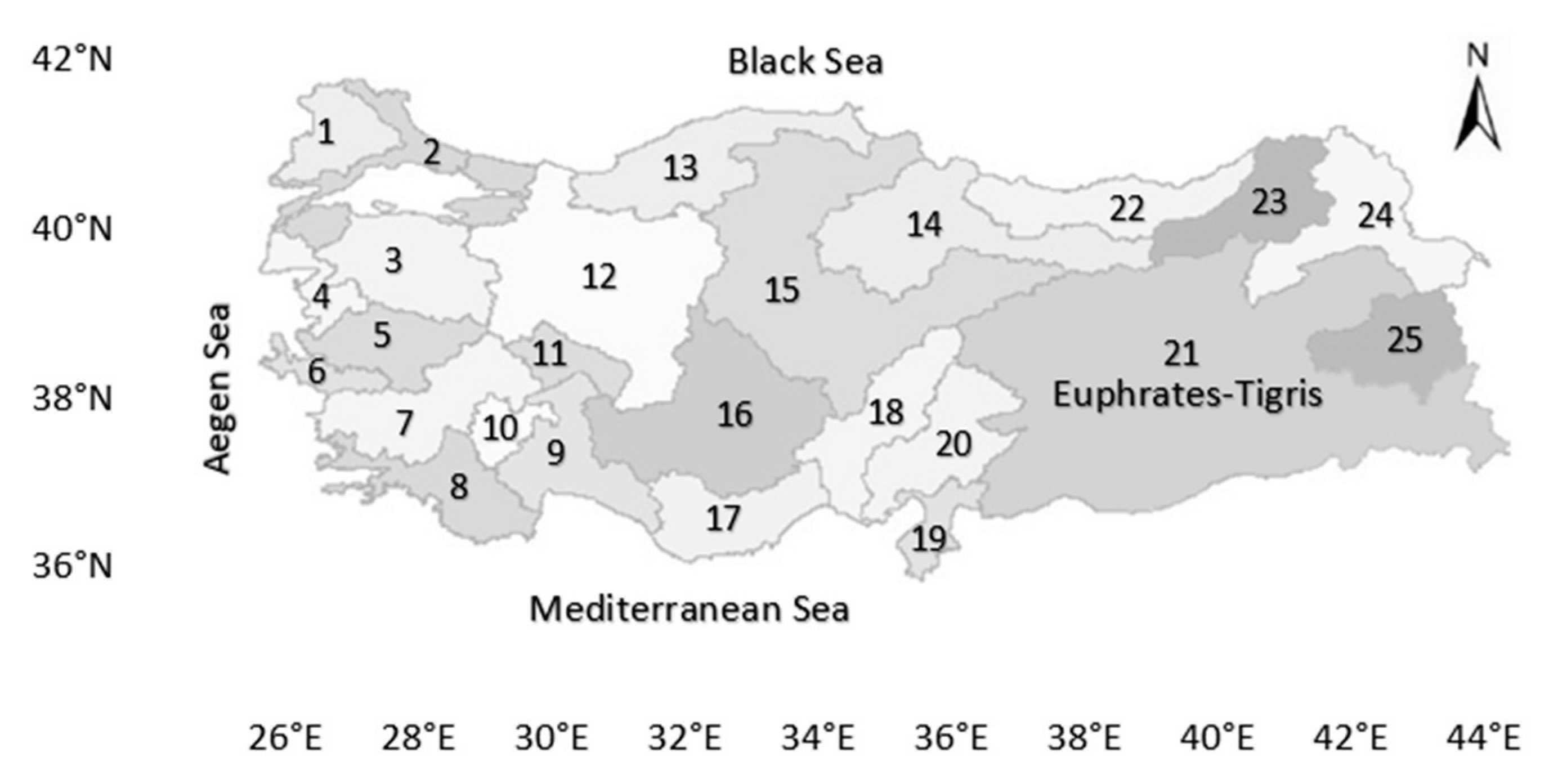
Turkey is divided into 25 hydrological river basins, where the Euphrates-Tigris (indicated with basin number 21) is regarded as one single basin (Figure 1). Euphrates-Tigris Basin is located in the eastern part of Turkey with a drainage area of 185,000 km², which is the largest basin of Turkey. It has also nearly 28.5% of the water potential of Turkey. As the biggest water source of the Euphrates-Tigris Basin, the Euphrates River is the longest and one of the most historically significant rivers of the Middle East. The total length of Euphrates is nearly 2800 km, and 40% of its length is in Turkey, 25% is in Syria, and 35% is in Iraq. The Euphrates River consists of two major tributaries, the Karasu River and the Murat River, which both originate in the Eastern Anatolia mountains of Turkey. These two rivers merge near the Keban Dam, which is one of the largest dams of Turkey. The Euphrates River Basin is subdivided into the Upper Euphrates, the Middle Euphrates, and the Lower Euphrates basins, which have some distinctive physical features. The water regime of the Euphrates River Basin depends heavily on winter rainfalls and spring snowmelt.

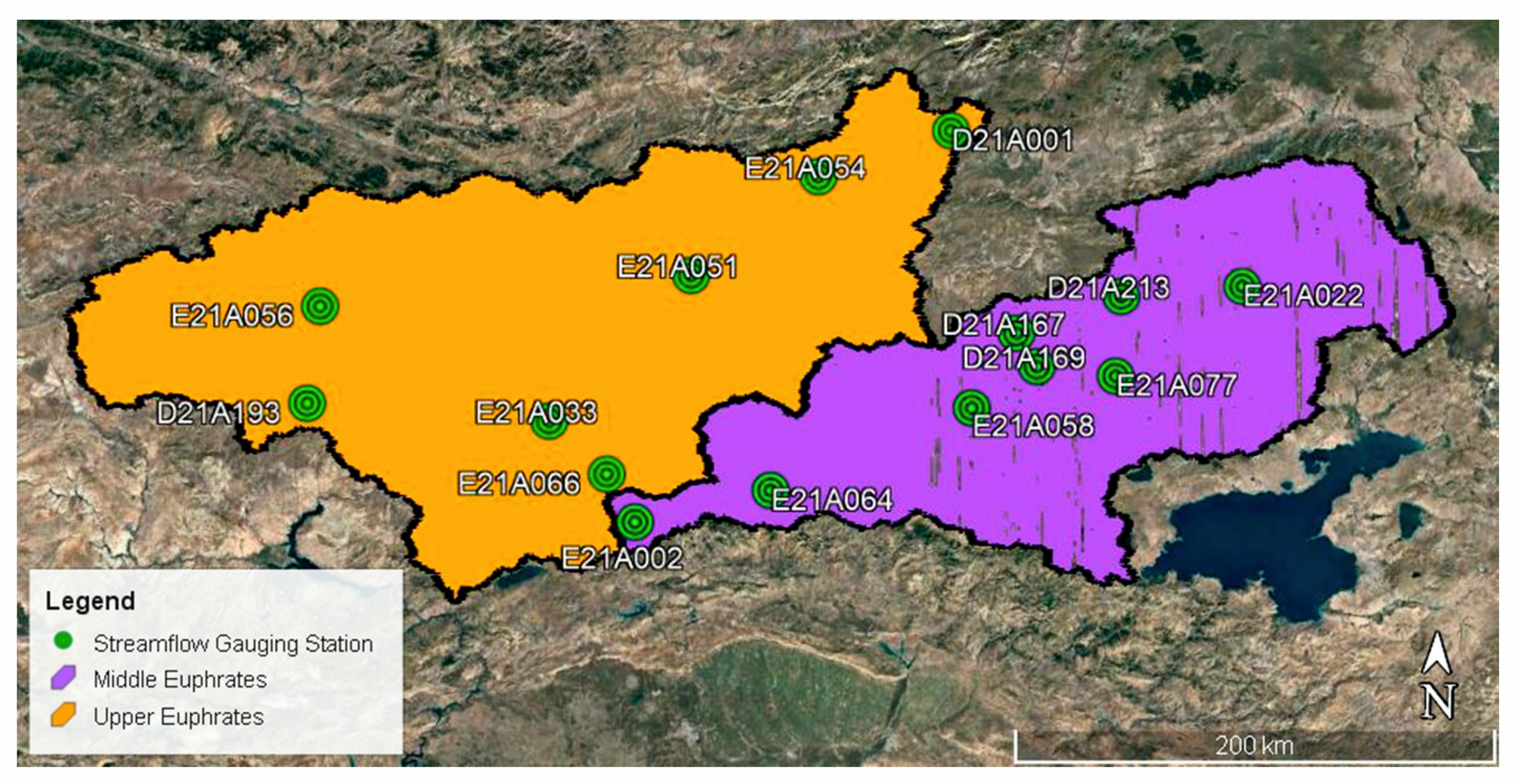
In order to determine the water potential of the Euphrates-Tigris Basin, a large number of streamflow gauging stations were established on the Euphrates River and its tributaries. However, there was a large amount of missing data in the daily streamflow measurements of some streamflow gauging stations. These missing data lead to significant problems in hydrological modeling studies. Statistical estimation methods require the use of daily streamflow time series obtained from a large number of streamflow gauging stations within the study area. Also, the observation period should be the same for all these streamflow gauging stations. In the Euphrates Basin as a case study, a total of 15 streamflow gauging stations, which have 24 years (1986–2009) of common daily streamflow data, was selected. Eight of these stations are located in the Middle Euphrates Basin, and the other seven stations are located in the Upper Euphrates Basin (Figure 2). Moreover, they are not located downstream of a dam.

2.2. Hydrological and Meteorological Data

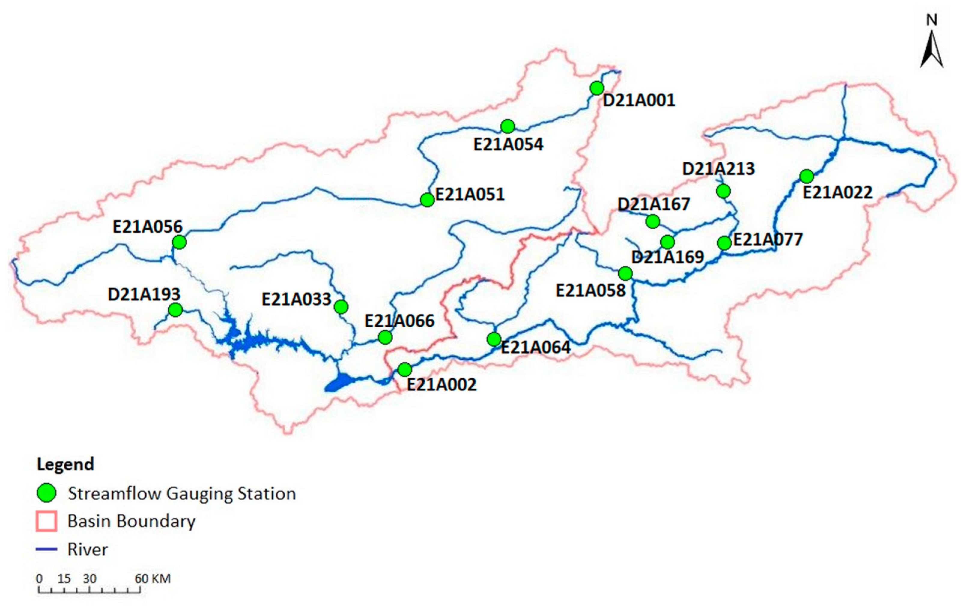
Eight streamflow gauging stations from the Middle Euphrates Basin and seven streamflow gauging stations from the Upper Euphrates Basin were selected for this case study. The stream networks of these two basins and the locations of the selected streamflow gauging stations in each basin are shown in Figure 3. Continuous daily streamflow data of the streamflow gauging stations operated by the General Directorate of State Hydraulic Works (DSI) were used. Each streamflow gauging station contains a 24-year period spanning from 1986 to 2009, and there is no missing data within the streamflow time series. The main characteristics of these streamflow gauging stations are listed in

Table 1. Characteristics of streamflow gauging stations in the Middle Euphrates Basin.

Station Number	Drainage Area (km2)	Elevation (m)	Long-Term Mean (m3/s)	Record Period (Years)
D21A167	250	1650	3.55	1986–2009
D21A169	276.1	1600	3.35	1986–2009
D21A213	65.3	1810	0.74	1986–2009
E21A002	25,515.6	852	239.82	1986–2009
E21A022	5882.4	1552	48.20	1986–2009
E21A058	1577.6	1310	18.91	1986–2009
E21A064	2232	990	32.97	1986–2009
E21A077	2995.3	1452	29.94	1986–2009

and

Table 2. Characteristics of streamflow gauging stations in the Upper Euphrates Basin.

Station Number	Drainage Area (km2)	Elevation (m)	Long-term Mean (m3/s)	Record Period (Years)
D21A001	233.2	1830	2.75	1986–2009
D21A193	518.1	1000	6.31	1986–2009
E21A033	3284.8	875	89.38	1986–2009
E21A051	8185.6	1355	60.23	1986–2009
E21A054	2886	1675	19.68	1986–2009
E21A056	15,562	865	153.57	1986–2009
E21A066	5430	840	78.26	1986–2009

. As shown by Table 1, drainage areas of the stations in the Middle Euphrates Basin vary between 65.3 and 25,515.6 km² whereas their elevations range between 852 and 1810 m above sea level. As shown by Table 2, drainage areas of the stations in the Upper Euphrates Basin vary between 233.2 and 15,562 km² whereas their elevations range between 840 and 1830 m above sea level.

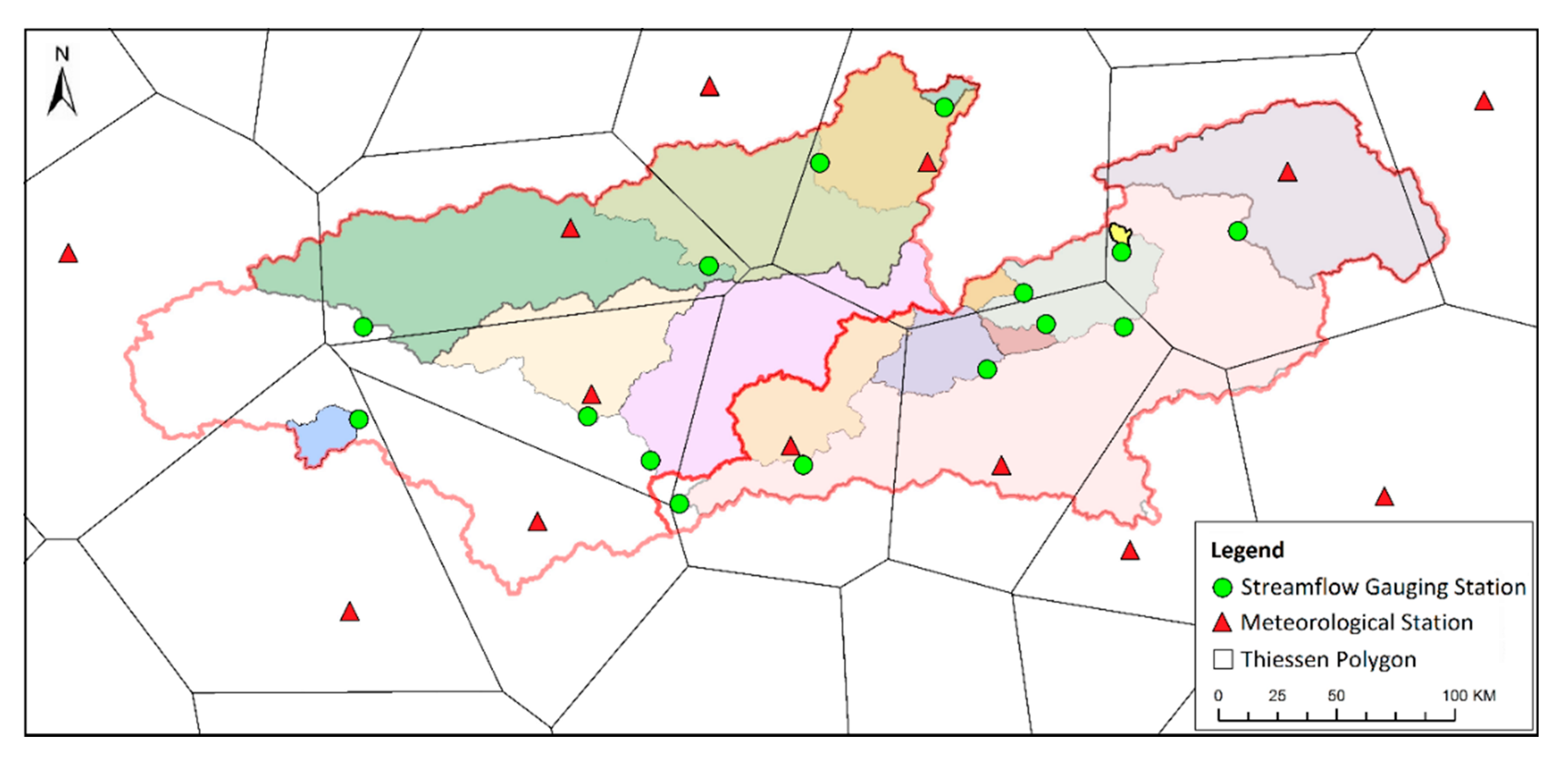
Basin characteristics such as geographical, topographical, and climate variables were considered for determining the physical similarity between the donor and target stations. Annual mean total precipitation and annual mean temperature were selected as climatic variables. Concurrent precipitation and temperature data of the meteorological stations operated by the Turkish State Meteorological Service (DMI) were used. The annual mean total precipitation and annual mean temperature values for each streamflow gauging station were calculated by the Thiessen polygon method (Figure 4). Thus, annual mean total precipitation and annual mean temperature values of the drainage area represented by each streamflow gauging station were obtained using the precipitation and temperature data of the meteorological stations. Drainage area, elevation, basin slope, and channel length were selected as topographical variables. Basin slope and channel length for the drainage basin of each streamflow gauging station were extracted using geographic information system (GIS) software. The latitude and longitude were selected as geographical variables because geographically nearby streamflow gauging stations could have similarities in hydrological behavior. They were converted to decimal degrees and then used to calculate the similarity coefficient. Since the latitude and longitude define the geographical location of the streamflow gauging stations, these selected basin characteristics combine the physical similarity approach with the geographical proximity approach [43]. Descriptive statistics of the selected physical characteristics are presented in

Table 3. Statistics of physical characteristics used in the Middle Euphrates Basin.

Physical Characteristics	Maximum	Minimum	Mean
Drainage Area (km2)	25,515.6	65.3	4849.3
Elevation (m)	1810	852	1402
Annual Mean Total Precipitation (mm)	939.50	431.20	679.68
Annual Mean Temperature (°F)	53.60	42.26	47.29
Basin Slope (%)	2.69	0.19	1.21
Channel Length (km)	565.11	14.75	142.27
Latitude (°)	39.54	38.69	39.19
Longitude (°)	42.78	39.93	41.58

for the Middle Euphrates Basin and in

Table 4. Statistics of physical characteristics used in the Upper Euphrates Basin.

Physical Characteristics	Maximum	Minimum	Mean
Drainage Area (km2)	15,562	233.2	5157.1
Elevation (m)	1830	840	1205.7
Annual Mean Total Precipitation (mm)	840.17	374.90	524.15
Annual Mean Temperature (°F)	56.48	42.26	48.52
Basin Slope (%)	2.82	0.16	0.96
Channel Length (km)	381.60	25.10	161.19
Latitude (°)	40.11	38.86	39.44
Longitude (°)	41.39	38.41	39.79

for the Upper Euphrates Basin.

3. Methods

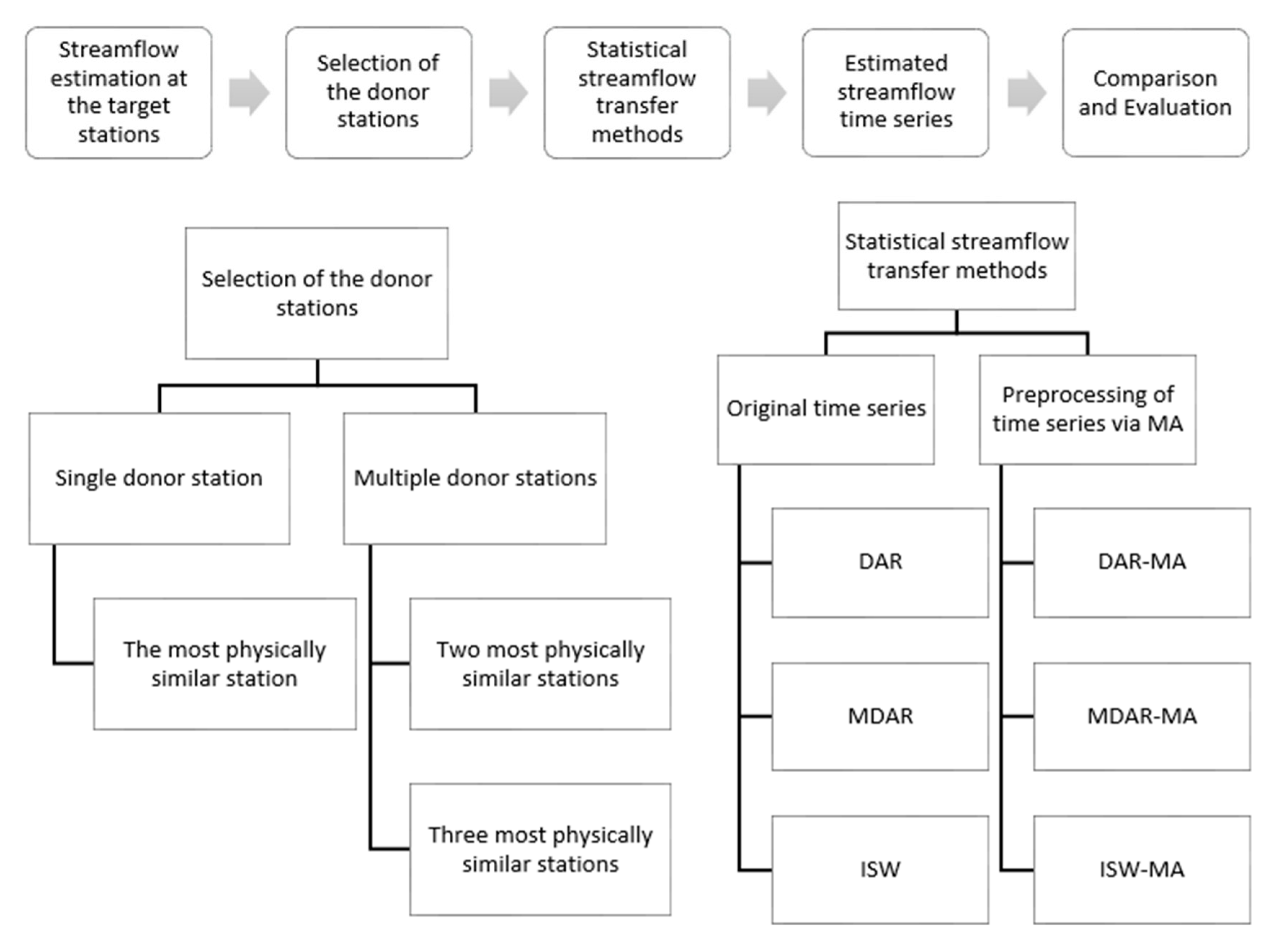
Estimation of daily streamflow time series at the target station consists of the following steps: (1) the selection of hydrologically similar donor stations to the target station and (2) the transfer of the daily streamflow time series from the donor station to target station by using statistical streamflow transfer methods. Proposed flowcharts for streamflow estimation at the target station are illustrated in Figure 5.

3.1. Statistical Information Transfer Methods

For daily streamflow estimation at the target stations, three statistical streamflow transfer methods are considered in this study. These methods include the single-donor station drainage area ratio (DAR) method, the multiple-donor stations drainage area ratio (MDAR) method, and the inverse similarity weighted (ISW) method. Moreover, the variations of the ISW method, in which constant power parameters are modified, are utilized as well. The DAR and the MDAR methods were based on the drainage area of the stations, whereas the ISW method was based on the physical similarity between the donor and target stations. Each statistical method is briefly described below.

3.1.1. Drainage Area Ratio (DAR) Method

The DAR method [39,40] assumes that the streamflow per unit drainage area for the target station equals that at the streamflow gauging station used as a donor station for a given day, as described in Equation (1).

$$Q_{target}=\frac{A_{target}}{A_{donor}}{Q}_{donor}$$

(1)

where $Q_{target}$ is the daily streamflow for the target station, $Q_{donor}$ is the streamflow at a donor station, and $A_{target}$ and $A_{donor}$ are the drainage areas for the target station and the donor station, respectively.

3.1.2. Multiple-Donor Stations Drainage Area Ratio (MDAR) Method

The MDAR method [2,32] generates the streamflow estimation at the target station as the weighted average of the DAR method estimations from the donor stations. The streamflow at the target station from the n donor stations can be calculated for a given day using Equation (2).

$$Q_{target}=\frac{{\sum }_{i=1}^n{w}_i{\widehat{Q}}_{dono{r}_i}}{{\sum }_{i=1}^n{w}_i}$$

(2)

where $w_i$ is the weight of the donor station i on the target station, ${\widehat{Q}}_{dono{r}_i}$ is the daily streamflow estimations from each donor station, and n is the total number of the donor stations. The values of the weights in Equation (2) which show the similarity between the target station and donor station can be calculated as Equation (3).

$$w_i=\frac{\frac{1}{d_i}}{{\sum }_{i=1}^n\frac{1}{d_i}}$$

(3)

where $d_i$ is the similarity distance between the target station and donor station i. The drainage area is frequently considered as the most important variable in many hydrological regionalization studies [39,40,44]. Moreover, the drainage area is also the only scaling factor used in the DAR method for streamflow estimation at the target stations. Therefore, it was used as the similarity distance in this study. It can be calculated using Equation (4).

$$d_i=\left|A_{target}-A_{dono{r}_i}\right|$$

(4)

where $A_{dono{r}_i}$ is the drainage area of the donor station i and $A_{target}$ is the drainage area of the target station.

3.1.3. Inverse Similarity Weighted (ISW) Method

The ISW method [37,38] estimates streamflow values at the target station as the weighted average of the streamflow values at n donor stations. The weights are inversely proportional to the power of physical similarity from the target station. The mathematical expression of the ISW method is given by Equation (5).

$$q_{target}={\displaystyle \sum _{i=1}^n}{w}_i{q}_{dono{r}_i}and{Q}_{target}=q_{target}{A}_{target}$$

(5)

where $q_{target}$ is the area normalized streamflow (m³/s/km²) at the target station and $q_{dono{r}_i}$ is the area normalized streamflow (m³/s/km²) at the donor station i. The weights $w_i$ based on physical similarity can be calculated for all donor stations using Equation (6). The sum of the weights assigned to each donor station is equal to 1.

$$w_i=\frac{\frac{1}{{s_i}^p}}{{\sum }_{i=1}^n\frac{1}{{s_i}^p}}and{\displaystyle \sum _{i=1}^n}{w}_i=1$$

(6)

where $s_i$ is the similarity coefficient between the target station and donor station i and where the exponent p is called a power parameter (p > 0). In this study, the estimation performance of the ISW method was evaluated using different power parameters from 1 to 3. For power parameters of 1, 2, and 3, the ISW method was referred to as ISW1, ISW2, and ISW3, respectively.

The similarity coefficient, s, is used to define the physical similarity between the target station and the donor station, which is calculated using Equation (7) [43,45]. Drainage area, elevation, annual mean total precipitation, annual mean temperature, basin slope, channel length, latitude, and longitude were considered as the basin characteristics in order to measure the physical similarity between the donor station and the target station. The station with the lowest similarity coefficient was selected as the donor station. The similarity coefficient was used both to select the donor stations and to transfer streamflow from several donor stations as the weight.

$$s={\sum }_{i=1}^k\frac{\left|X_i^{donor}-X_i^{target}\right|}{max(X_i)-min(X_i)}$$

(7)

where i indicates one of a total of k selected basin characteristics; $X_i^{donor}$ and $X_i^{target}$ are the values of basin characteristic i for the donor station and the target station, respectively; and $max(X_i)$ and $min(X_i)$ are the maximum and the minimum values of basin characteristics over the set of stations considered, respectively.

3.2. Selection of Donor Stations

For transferring the streamflow to the target (ungauged) station, the streamflow values of the donor stations are used. Therefore, the selection of the donor stations is an important step in estimating streamflow at the target station. In this study, the physical similarity approach was considered to identify donor stations. In the physical similarity approach, the station that minimizes the similarity coefficient defined in Equation (7) was used as the donor station. That is, the best donor station was given to the station having the smallest s value. Although all stations are gauged, initially, each station in each basin was considered in turn as a target station and daily streamflow time series were estimated for all stations assumed as a target station within each basin. Subsequently, their actual streamflow time series were used in order to evaluate the performance of the streamflow estimation. When using one donor station, the most physically similar station was identified for each target station. On the other hand, when using more than one donor station, the two or three most physically similar stations were identified for each target station (Figure 5). Therefore, the DAR method was applied to each station using the most physically similar station as the donor station, while the MDAR and ISW methods were applied to each station for two different cases: 1) using the two most physically similar stations as the donor stations and 2) using the three most physically similar stations as the donor stations. The results for these two different cases were compared with the original observations to evaluate which one provides better estimation performance.

3.3. Data Preprocessing

The streamflow data may contain possible errors, and these errors are collectively referred to as noise. As the noise in the data increases, reliable results will be difficult to achieve. In this study, data preprocessing was conducted to remove noise and to improve the reliability of daily streamflow estimates. The data preprocessing discussed here was daily streamflow data smoothing using the moving average (MA). Each daily streamflow time series of all stations was smoothed by a centered (or symmetric two-sided) moving average of length m = 2k + 1, i.e., MA(m), and then, the smoothed streamflow time series were used into the statistical methods. Hereafter, the statistical methods, DAR, MDAR, and ISW are referred to as DAR-MA, MDAR-MA, and ISW-MA, respectively. A centered moving average smooths data by replacing each observed daily streamflow value with the average of the current day, previous day, and subsequent days and is defined as Equation (8). For example, a centered moving average of length m = 3 (hence k = 1), i.e., MA(3) with equal weights, replaces the observed daily streamflow value $x_t$ at time t with the averages of $x_{t-1}$, $x_t$, and $x_{t+1}$.

$$x_t^{*}=\frac{1}{2k+1}{\displaystyle \sum _{i=-k}^k}{x}_{t+i}$$

(8)

where $x_t^{*}$ is the smoothed streamflow value at time t and m = 2k + 1 is the number of observed values that are averaged.

In order to smooth daily streamflow data, MA was applied with lengths of 3, 5, 7, 9, and 11 days in this study, and then, it was seen that the larger the length m = 2k + 1, the more the streamflow peaks (maximum values) and streamflow valleys (minimum values) were smoothed out. The peaks and valleys of streamflow are not well represented by the relatively high length of MA(5), MA(7), MA(9), and MA(11). For a better representation of streamflow peaks and valleys, MA(5), MA(7), MA(9), and MA(11) were excluded from the rest of the study.

3.4. Evaluation Criteria

A jackknife (leave one out) procedure was used for evaluating the performance of each method. In this procedure, each station in each basin was considered in turn as a target station and was removed from the database. This procedure was repeated for all stations considered for this study.

The performance of each statistical method was evaluated in terms of the Nash–Sutcliffe efficiency (NSE) [46], the ratio of the root mean square error (RMSE) to the standard deviation of the observed data (RSR) [47], the percent bias (PBIAS), and the coefficient of determination (R²) between the estimated and observed streamflow values. NSE, RSR, PBIAS, and R² were calculated as follows:

$$NSE=1-\frac{{\sum }_{i=1}^n{\left(X_i^{obs}-X_i^{est}\right)}^2}{{\sum }_{i=1}^n{(X_i^{obs}-{\overline{X}}^{obs})}^2}$$

(9)

$$RSR=\frac{RMSE}{\sqrt{\frac{{\sum }_{i=1}^n{\left(X_i^{obs}-{\overline{X}}^{obs}\right)}^2}{n}}}=\frac{\sqrt{{\sum }_{i=1}^n{\left(X_i^{obs}-X_i^{est}\right)}^2}}{\sqrt{{\sum }_{i=1}^n{(X_i^{obs}-{\overline{X}}^{obs})}^2}}=\sqrt{1-NSE}$$

(10)

$$PBIAS=\frac{{\sum }_{i=1}^n\left(X_i^{obs}-X_i^{est}\right)}{{\sum }_{i=1}^n\left(X_i^{obs}\right)}x100$$

(11)

$$R^2={\left(\frac{{\sum }_{i=1}^n(X_i^{obs}-{\overline{X}}^{obs})(X_i^{est}-{\overline{X}}^{est})}{\sqrt{{\sum }_{i=1}^n{(X_i^{obs}-{\overline{X}}^{obs})}^2}\sqrt{{\sum }_{i=1}^n{(X_i^{est}-{\overline{X}}^{est})}^2}}\right)}^2$$

(12)

where $X_i^{obs}$ is the ith observed daily streamflow value; $X_i^{est}$ is the ith estimated daily streamflow value; ${\overline{X}}^{obs}$ and ${\overline{X}}^{est}$ are the mean of observed and estimated daily streamflow values, respectively; and n is the total number of observed daily streamflow values.

The NSE values range between −∞ and +1, where a value of 1 indicates a perfect agreement between estimated and observed streamflow values. The values closer to 1 indicate an increasingly better agreement, whereas the values far from 1 indicate an increasingly poor agreement. The RSR standardizes RMSE using the standard deviation of the observed data. The RSR varies from the optimal value of 0 to a large positive value. The lower the RSR, the better the performance of the method [47]. PBIAS measures the average tendency of the estimated values to be larger or smaller than corresponding observed values. The optimal value of PBIAS is 0, and the closer it is to 0, the more accurate the estimated values are to the observed values. Negative PBIAS values indicate overestimation, while positive PBIAS values indicate underestimation [47]. The coefficient of determination (R²) is the square of the correlation coefficient according to Pearson. The R² values range from 0 to 1, with higher values indicating better agreement between estimated and observed values. Generally, R² values greater than 0.5 are considered acceptable [47].

Moriasi et al. [47] suggested performance ratings of recommended statistics such as NSE, RSR, and PBIAS for monthly streamflow. According to Moriasi et al. [47], the performance of the method is considered satisfactory when the NSE is greater than 0.5, the RSR is less than 0.7, and the PBIAS ranges are less than ±25%. However, NSE values lower than 0.5 for daily streamflow can still be considered satisfactory [48]. Therefore, some of the constraints for the recommended statistics can be relaxed for daily streamflow. In this study, the adjusted performance ratings of the NSE and PBIAS statistics for the daily time scale proposed by Kalin et al. [49] were used to evaluate the performance of the statistical methods (

Table 5. Performance ratings of the Nash–Sutcliffe efficiency (NSE) and percent bias (PBIAS) statistics for daily streamflow.

Performance Rating	NSE	abs(PBIAS) %
Very good	NSE ≥ 0.7	abs(PBIAS) ≤ 25
Good	0.5 ≤ NSE < 0.7	25 < abs(PBIAS) ≤ 50
Satisfactory	0.3 ≤ NSE < 0.5	50 < abs(PBIAS) ≤ 70
Unsatisfactory	NSE < 0.3	abs(PBIAS) > 70

).

4. Results and Discussion

4.1. Middle Euphrates Basin

The statistical methods described above were applied on each of eight streamflow gauging stations in the Middle Euphrates Basin, which were considered in turn as the target station. The donor station or stations based on physical similarity was selected to transfer daily streamflow data to the target station.

Table 6. Physically similar donor stations for each target station in the Middle Euphrates Basin.

Target Station	Donor Station
	1st	2nd	3rd	4th	5th	6th	7th
D21A167	D21A213	D21A169	E21A022	E21A058	E21A077	E21A064	E21A002
D21A169	E21A058	E21A077	D21A167	D21A213	E21A022	E21A064	E21A002
D21A213	D21A167	E21A022	D21A169	E21A058	E21A077	E21A064	E21A002
E21A002	E21A064	E21A058	E21A077	E21A022	D21A169	D21A167	D21A213
E21A022	D21A213	E21A077	D21A167	E21A058	D21A169	E21A064	E21A002
E21A058	E21A077	D21A169	E21A064	E21A022	D21A167	D21A213	E21A002
E21A064	E21A058	E21A077	D21A169	E21A002	E21A022	D21A167	D21A213
E21A077	E21A058	D21A169	E21A022	E21A064	D21A213	D21A167	E21A002

shows the sequence of the donor stations for each target station in the Middle Euphrates Basin which was determined according to the similarity coefficient.

In order to estimate daily streamflow at the target stations, the DAR method was applied by using the most physically similar station to each target station. In order to test the applicability of the donor station selection criteria for the study area, the NSE values were determined for the donor stations identified by the physical similarity and compared with the NSE values obtained from the donor stations traditionally selected as the geographically nearest stations. On the other hand, the MDAR and ISW methods were applied by using the two and the three most physically similar stations to each target station. In order to test the effect of different power parameter selection in the use of the ISW method on the accuracy of daily streamflow estimation, the ISW method was applied with power parameters of 1, 2, and 3. In addition, the comparisons between the statistical methods with and without the MA were carried out to indicate the effectiveness of the MA-based preprocessing on the accuracy of daily streamflow estimation. Daily streamflow values estimated using both observed and smoothed data from the donor stations were compared with observed data at the target station. According to the selection criteria of the donor stations, the NSE values obtained for the target stations in the Middle Euphrates Basin are given in

Table 7. NSE values for the drainage area ratio (DAR) and multiple-donor stations drainage area ratio (MDAR) methods in the Middle Euphrates Basin.

Target Station	The Geographically Nearest Donor Station	The Most Physically Similar Donor Station	Two Most Physically Similar Donor Stations	Three Most Physically Similar Donor Stations
	DAR	DAR	MDAR	MDAR
D21A167	0.313	−0.187	0.312	0.316
D21A169	0.581	0.850	0.852	0.595
D21A213	0.718	0.354	0.369	0.608
E21A002	−0.171	−0.171	0.433	0.729
E21A022	−0.205	−0.205	0.622	0.718
E21A058	0.826	0.814	0.894	0.839
E21A064	0.649	0.724	0.694	0.706
E21A077	0.300	0.647	0.651	0.781

for DAR and MDAR and in

Table 8. NSE values for the inverse similarity weighted (ISW) with powers of 1, 2, and 3 in the Middle Euphrates Basin.

Target Station	Two Most Physically Similar Donor Stations			Three Most Physically Similar Donor Stations
	ISW1	ISW2	ISW3	ISW1	ISW2	ISW3
D21A167	0.136	0.060	−0.009	0.317	0.184	0.065
D21A169	0.844	0.849	0.852	0.816	0.825	0.833
D21A213	0.501	0.463	0.429	0.608	0.556	0.502
E21A002	0.418	0.396	0.374	0.696	0.664	0.630
E21A022	0.432	0.375	0.316	0.636	0.591	0.535
E21A058	0.893	0.892	0.892	0.904	0.907	0.906
E21A064	0.696	0.701	0.706	0.712	0.713	0.714
E21A077	0.641	0.651	0.656	0.774	0.743	0.716

for ISW with three different power parameters (1, 2, and 3). Performance evaluations of the best statistical method without and with the MA for each target station in the Middle Euphrates Basin are presented in

Table 9. Performance evaluation of the best statistical method without the moving average (MA) for each target station in the Middle Euphrates Basin.

Target Station	Method	NSE	RSR	PBIAS
D21A167	ISW1	0.317 3	0.827	23.265 1
D21A169	ISW3	0.852 1	0.385	6.459 1
D21A213	ISW1	0.608 2	0.626	−6.122 1
E21A002	MDAR	0.729 1	0.520	−30.114 2
E21A022	MDAR	0.718 1	0.531	−39.089 2
E21A058	ISW2	0.907 1	0.304	3.123 1
E21A064	DAR	0.724 1	0.525	18.865 1
E21A077	MDAR	0.781 1	0.468	−11.015 1

¹ Very good, ² good, ³ satisfactory, and ⁴ unsatisfactory.

and in

Table 10. Performance evaluation of the best statistical method with the MA for each target station in the Middle Euphrates Basin.

Target Station	Method	NSE	RSR	PBIAS
D21A167	ISW1-MA	0.326 3	0.821	23.265 1
D21A169	ISW3-MA	0.876 1	0.352	6.459 1
D21A213	ISW1-MA	0.618 2	0.618	−6.122 1
E21A002	MDAR-MA	0.767 1	0.483	−30.114 2
E21A022	MDAR-MA	0.725 1	0.524	−39.089 2
E21A058	ISW2-MA	0.921 1	0.282	3.123 1
E21A064	DAR-MA	0.744 1	0.506	18.865 1
E21A077	MDAR-MA	0.817 1	0.428	−11.015 1

¹ Very good, ² good, ³ satisfactory, and ⁴ unsatisfactory.

, respectively.

For 2 out of 8 target stations (i.e., E21A002 and E21A022), the geographically nearest and the most physically similar station were the same. For 3 out of the remaining 6 target stations (i.e., D21A169, E21A064, and E21A077), higher NSE values were obtained using DAR with the most physically similar station as the donor station. For 3 out of the target stations (i.e., D21A167, D21A213, and E21A058), higher NSE values were obtained using DAR with the geographically nearest station as the donor station. According to these results, for half of the target stations in the study area, the geographical distance seems to be a good selection criterion as the donor station; however, for the remaining half of the target stations, geographical distance cannot identify the best donor station. Therefore, donor station selection criteria can provide different estimated results that vary from basin to basin.

As can be seen in Table 7, for all target stations other than E21A064, higher NSE values were obtained with MDAR compared with DAR. Especially for D21A167, E21A002, and E21A022, negative NSE values obtained with DAR using the most physically similar donor station improved considerably when the three most physically similar donor stations were used with MDAR. The performance of the DAR method was unsatisfactory for D21A167, E21A002, and E21A022. This was mostly due to the significant increase in the drainage area ratio between the donor and target stations. D21A213 has the smallest drainage area (65.3 km²) in the Middle Euphrates Basin and was determined as the most physically similar donor station for both D21A167 (250 km²) and E21A022 (5882.4 km²). Moreover, E21A002 has the largest drainage area (25,515.6 km²) in the Middle Euphrates Basin. Its drainage area is more than four times the next largest station. For all target stations other than D21A169 and E21A058, MDAR using of the three most physically donor stations produced better NSE values than that using the two most physically similar donor stations. For D21A169, the NSE value decreased from 0.852 to 0.595 when the three most physically similar donor stations were used instead of the two most physically similar donor stations (see Table 7). In case of the use of the three most physically similar donor stations, the third most physically similar donor station for D21A169 was determined as D21A167. The NSE value obtained for D21A169 using the DAR method and utilizing D21A167 was lower than the NSE values obtained from the other two donor stations (i.e., E21A058 and E21A077). The drainage area of the donor station D21A167 is very close to the target station D21A169. On the other hand, the drainage areas of the other two donor stations are much larger than D21A169. Hence, the weight of donor station D21A167 for streamflow estimation of D21A169 is significantly larger compared to the other two. Consequently, the NSE value obtained for D21A169 using MDAR with the three most physically similar donor stations is predominantly influenced by donor station D21A167. Similarly, for E21A058, the decrease in the NSE (i.e., from 0.894 to 0.839) was due to the same reason as for D21A169.

As can be seen in Table 8, in case of the use of the two most physically similar donor stations, the best performance results were obtained with ISW1 for 5 out of 8 target stations (i.e., D21A167, D21A213, E21A002, E21A022, and E21A058). On the other hand, in case of the use of the three most physically similar donor stations, the best performance results were obtained with ISW1 for 5 out of 8 target stations (i.e., D21A167, D21A213, E21A002, E21A022, and E21A077). In both cases, the most reasonable estimation results were mostly obtained when ISW1 was applied instead of ISW2 and ISW3. Moreover, the NSE values mostly improved when the three most physically similar donor stations were used instead of the two most physically similar donor stations.

As can be seen in Table 9, for all target stations other than for E21A064, the MDAR and the ISW methods resulted in higher NSEs compared to the DAR method. For 6 out of 8 target stations, the results can be rated as “very good” for NSE according to the performance ratings in Table 5. For 7 out of 8 target stations, the RSR values were considered satisfactory (i.e., less than 0.7) according to the performance ratings recommended by Moriasi et al. [47]. The negative PBIAS values for D21A213, E21A002, E21A022, and E21A077 demonstrate that the method overestimated daily streamflow, while positive PBIAS values for D21A167, D21A169, E21A058, and E21A064 demonstrate underestimation. For all target stations, the statistical methods with the MA tend to achieve slightly higher NSE values. However, the PBIAS values of the target stations did not change when the statistical methods with the MA were used.

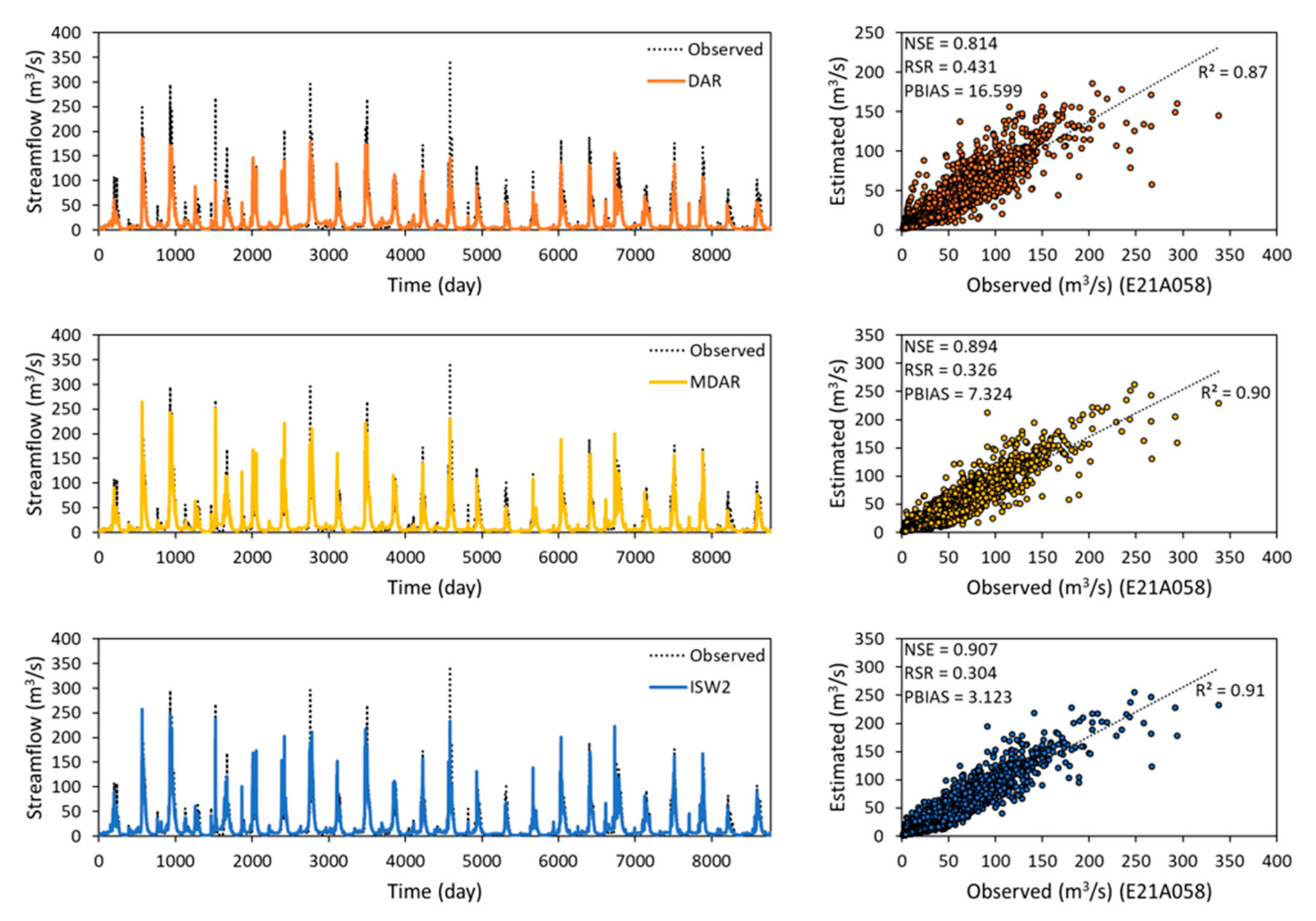
For the target station E21A058 as the example, the estimated daily streamflow values from the statistical methods without MA were compared to the observed (original) daily streamflow values in the hydrograph and scatter plots in Figure 6. The remarkably better agreement between observed and estimated daily streamflow values by three statistical methods (i.e, DAR, MDAR, and ISW) was obtained for E21A058 compared to the other target stations in the Middle Euphrates Basin. ISW2 gave a coefficient of determination (R²) of 0.91, which was higher than the R² values of 0.87 and 0.90 obtained by using the DAR and MDAR, respectively. The NSE values for these methods ranged from 0.814 to 0.907, and the best NSE value was achieved by ISW2. The best NSE performance for E21A058 was obtained using ISW2 with the three most physically similar donor stations.

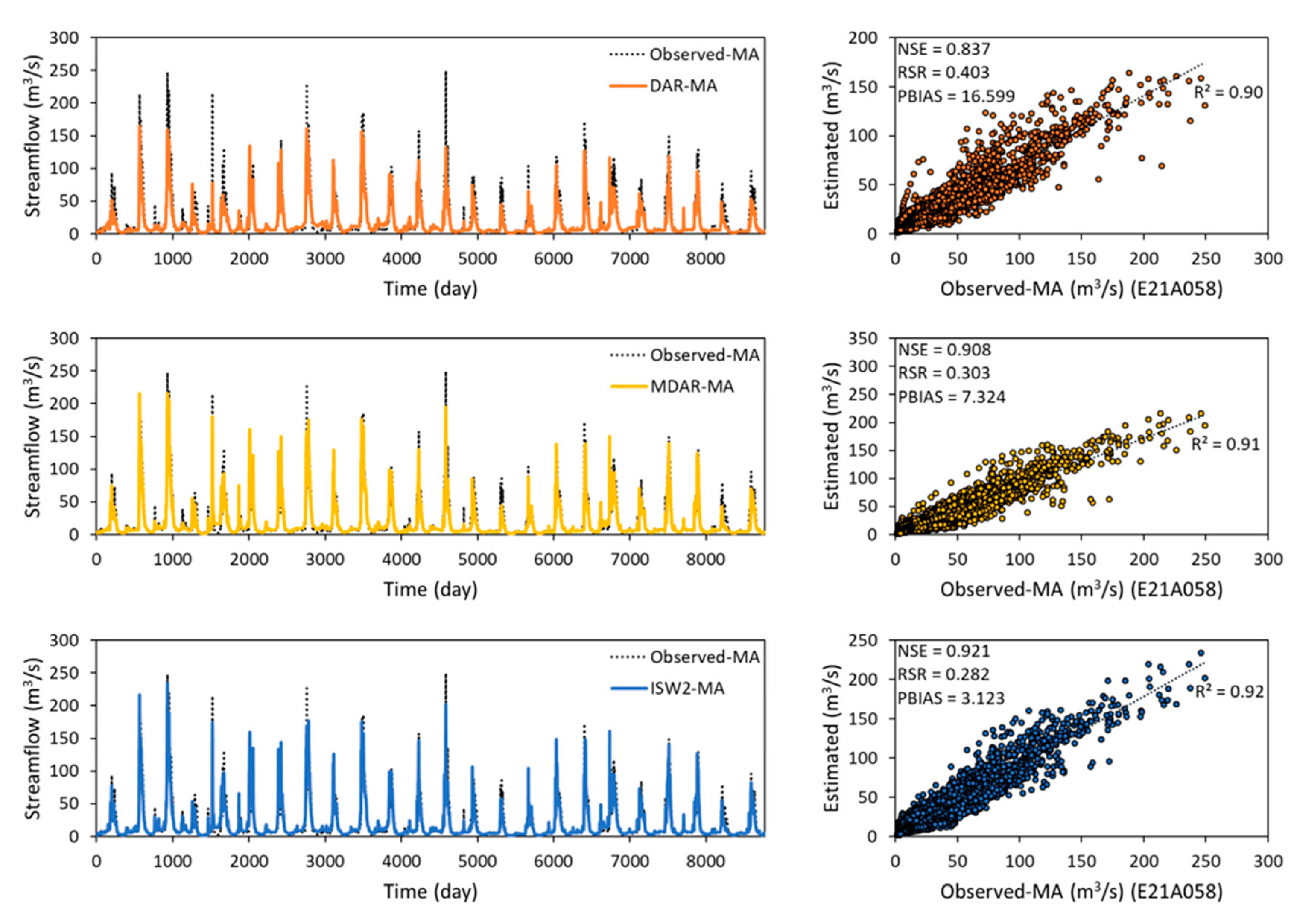
On the other hand, for the target station E21A058 as the example, the estimated daily streamflow values from the statistical methods with MA were compared with observed-MA (smoothed) daily streamflow values in the hydrograph and scatter plots in Figure 7. The statistical methods with MA performed slightly better for E21A058.

4.2. Upper Euphrates Basin

Using the same procedure applied for the Middle Euphrates Basin, the statistical methods were applied on each of seven streamflow gauging stations in the Upper Euphrates Basin for the purpose of estimating daily streamflow.

Table 11. Physically similar donor stations for each target station in the Upper Euphrates Basin.

Target Station	Donor Station
	1st	2nd	3rd	4th	5th	6th
D21A001	E21A054	E21A051	D21A193	E21A033	E21A033	E21A066
D21A193	E21A033	E21A066	E21A056	E21A051	E21A051	E21A054
E21A033	E21A066	D21A193	E21A051	E21A056	E21A056	D21A001
E21A051	E21A054	E21A056	E21A066	E21A033	E21A033	D21A193
E21A054	E21A051	D21A001	E21A033	E21A056	E21A056	D21A193
E21A056	E21A051	E21A066	E21A033	D21A193	D21A193	D21A001
E21A066	E21A033	E21A051	E21A056	D21A193	D21A193	D21A001

shows the sequence of the donor stations for each target station in the Upper Euphrates Basin which was determined according to the similarity coefficient.

According to the selection criteria of the donor stations, the NSE values obtained for the target stations in the Upper Euphrates Basin were given in

Table 12. NSE values for the DAR and MDAR methods in the Upper Euphrates Basin.

Target Station	The Geographically Nearest Donor Station	The Most Physically Similar Donor Station	Two Most Physically Similar Donor Stations	Three Most Physically Similar Donor Stations
	DAR	DAR	MDAR	MDAR
D21A001	0.619	0.619	0.630	−0.328
D21A193	0.299	−0.646	−0.053	0.089
E21A033	0.446	0.446	0.377	0.319
E21A051	0.883	0.883	0.932	0.362
E21A054	0.159	0.885	0.585	−5.128
E21A056	−3.199	0.769	0.415	−0.586
E21A066	−0.067	−0.067	0.698	0.732

for DAR and MDAR and in

Table 13. NSE values for ISW with powers of 1, 2, and 3 in the Upper Euphrates Basin.

Target Station	Two Most Physically Similar Donor Stations			Three Most Physically Similar Donor Stations
	ISW1	ISW2	ISW3	ISW1	ISW2	ISW3
D21A001	0.633	0.629	0.626	0.597	0.626	0.631
D21A193	0.015	−0.085	−0.185	0.307	0.217	0.108
E21A033	0.416	0.439	0.444	0.353	0.412	0.435
E21A051	0.931	0.928	0.921	0.811	0.877	0.905
E21A054	0.753	0.775	0.794	0.244	0.580	0.719
E21A056	0.404	0.541	0.640	−0.788	−0.306	0.083
E21A066	0.479	0.191	0.033	0.645	0.331	0.097

for ISW with three different power parameters (1, 2, and 3). Performance evaluations of the best statistical method without and with the MA for each target station in the Upper Euphrates Basin are presented in

Table 14. Performance evaluation of the best statistical method without the MA for each target station in the Upper Euphrates Basin.

Target Station	Method	NSE	RSR	PBIAS
D21A001	ISW1	0.633 2	0.606	40.537 2
D21A193	ISW1	0.307 3	0.832	−51.370 3
E21A033	DAR	0.446 3	0.744	47.035 2
E21A051	MDAR	0.932 1	0.261	−10.006 1
E21A054	DAR	0.885 1	0.339	−7.892 1
E21A056	DAR	0.769 1	0.480	25.436 2
E21A066	MDAR	0.732 1	0.518	−22.121 1

¹ Very good, ² good, ³ satisfactory, and ⁴ unsatisfactory.

and in

Table 15. Performance evaluation of the best statistical method with the MA for each target station in the Upper Euphrates Basin.

Target Station	Method	NSE	RSR	PBIAS
D21A001	ISW1-MA	0.646 2	0.595	40.537 2
D21A193	ISW1-MA	0.305 3	0.834	−51.371 3
E21A033	DAR-MA	0.453 3	0.740	47.035 2
E21A051	MDAR-MA	0.939 1	0.248	−10.006 1
E21A054	DAR-MA	0.897 1	0.322	−7.892 1
E21A056	DAR-MA	0.780 1	0.469	25.436 2
E21A066	MDAR-MA	0.749 1	0.501	−22.120 1

¹ Very good, ² good, ³ satisfactory, and ⁴ unsatisfactory.

, respectively.

For 2 out of the 3 target stations (i.e., E21A054 and E21A056) for which the geographically nearest and the most physically similar stations were not the same, higher NSE values were obtained using DAR with the most physically similar station (see Table 12). For E21A054 and E21A056, the NSE values improved considerably when the most physically similar station was used. These results indicate that the physical similarity may be a better selection criterion for the donor station in the study area compared to the geographical distance between the stations.

As can be seen in Table 12, for all target stations other than E21A033, E21A054, and E21A056, higher NSE values were obtained with MDAR compared with DAR. Especially for E21A066, the NSE value improved considerably with MDAR as compared with DAR. For D21A001, E21A051, E21A054, and E21A056, the NSE values decreased when MDAR was applied using the three most physically similar donor stations instead of the two most physically similar donor stations (see Table 12). In case of use of the three most physically similar donor stations, the third most physically similar donor stations for the target stations D21A001, E21A051, and E21A054 were determined as D21A193, E21A066, and E21A033, respectively. All NSE values obtained for these target stations using the DAR method utilizing their third most physically similar donor stations were negative. The drainage areas of these target stations and their third most physically similar donor stations are very close to each other. Therefore, the weight of their third most physically similar donor stations for streamflow estimation of these target stations is significantly larger. As a result, the NSE values obtained for the target stations D21A001, E21A051, and E21A054 using MDAR with three most physically similar donor stations are predominantly influenced by their third most physically similar donor stations. On the other hand, for E21A056, the reason is slightly different from the others. The NSE value obtained for E21A056 using the DAR method utilizing its third most physically similar donor station E21A033 was too low (i.e., −10.029). Although the contribution of the donor station E21A033 is not much more than the other two, this leads to poor estimation performance for E21A056 when MDAR was applied using the three most physically similar donor stations.

As can be seen in Table 13, in case of the use of the two most physically similar donor stations, the best performance results were obtained with ISW1 for 4 out of 7 target stations (i.e., D21A001, D21A193, E21A051, and E21A066). On the other hand, in case of the use of the three most physically similar donor stations, the best performance results were obtained with ISW3 for all target stations other than D21A193 and E21A066. As the power parameter increased from 1 to 3, the NSE values mostly improved when the three most physically similar donor stations were used, whereas the NSE values mostly decreased when the two most physically similar donor stations were used. Moreover, the NSE values mostly improved when the two most physically similar donor stations were used instead of the three most physically similar donor stations.

As can be seen in Table 14, for all target stations other than for E21A033, E21A054, and E21A056, the MDAR and the ISW methods resulted in higher NSE compared to the DAR method. For 4 out of 7 target stations, the results can be rated as “very good” for the NSE according to the performance ratings in Table 5. For 5 out of 7 target stations, the RSR values were considered satisfactory (i.e., less than 0.7) according to the performance ratings recommended by Moriasi et al. [47]. The negative PBIAS values for D21A193, E21A051, E21A054, and E21A066 demonstrate that the method overestimated daily streamflow, while positive PBIAS values for D21A001, D21A033, and E21A056 demonstrate underestimation. For all target stations other than D21A193, the statistical methods with MA tend to achieve slightly higher NSE values. However, the PBIAS values of the target stations did not change when the statistical methods with MA were used.

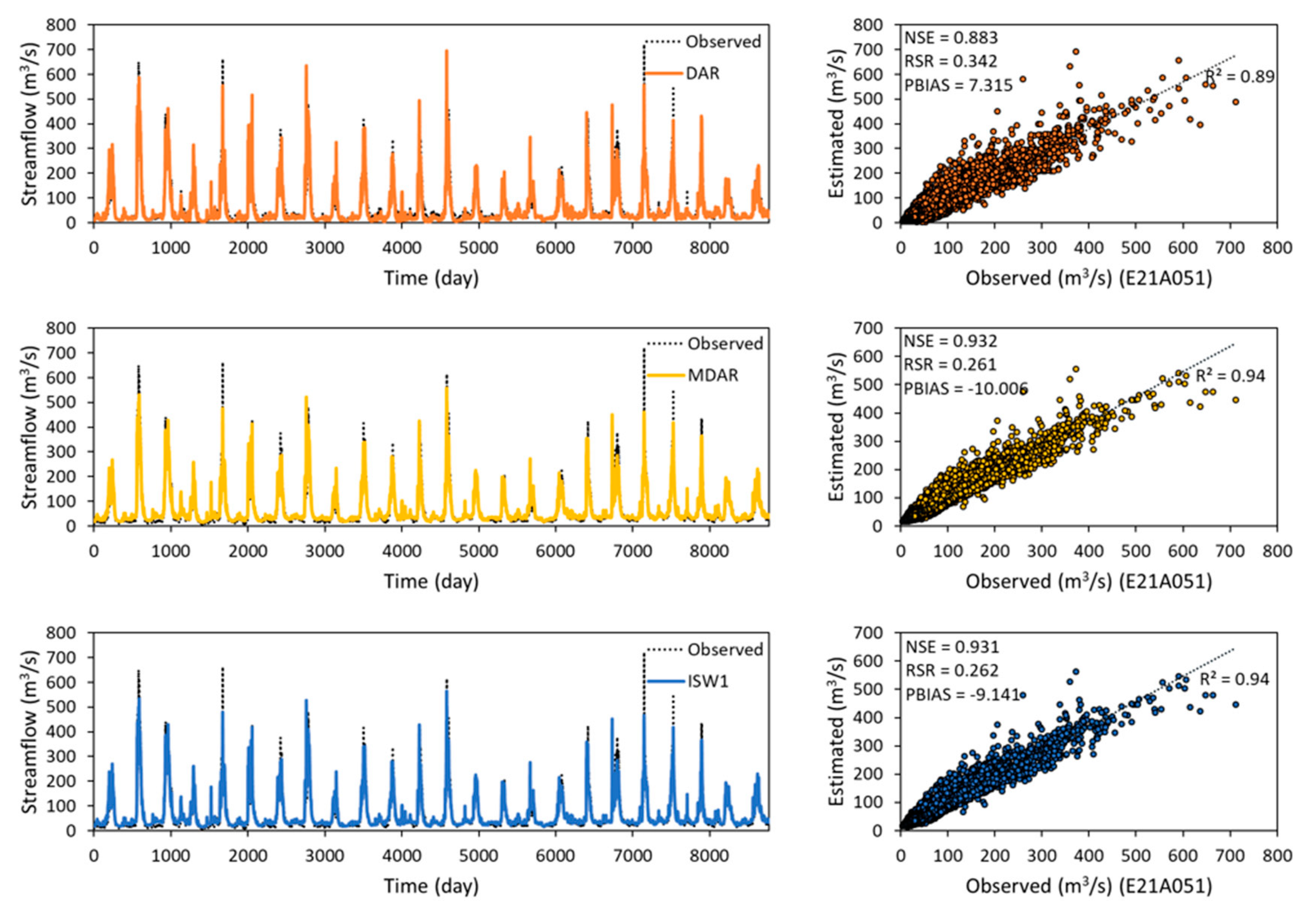
For the target station E21A051 as the example, the estimated streamflow values from the statistical methods without the MA were compared to observed (original) streamflow values in the hydrograph and scatter plots in Figure 8. The remarkably better agreement between observed and estimated streamflow values by three statistical methods was obtained for E21A051 compared to the other stations in the Upper Euphrates Basin. Both MDAR and ISW1 gave a coefficient of determination (R²) of 0.94, which was higher than the R² values of 0.89 by using DAR. The NSE values for these methods ranged from 0.883 to 0.932, and the best NSE value was achieved by MDAR. The best NSE performance for E21A051 was obtained using MDAR with the two most physically similar donor stations.

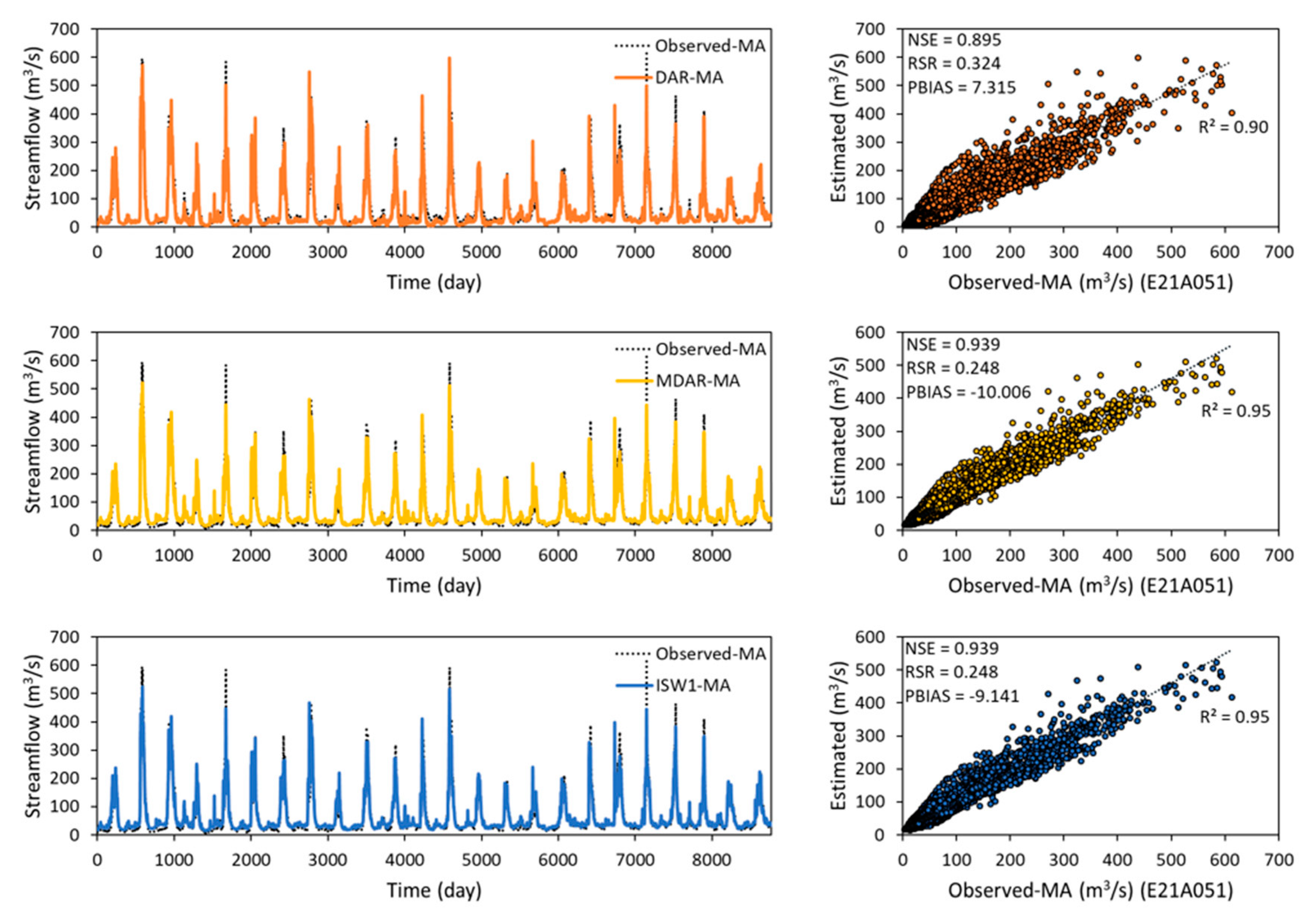
On the other hand, for the target station E21A051 as the example, the estimated streamflow values from the statistical methods with the MA were compared to observed-MA (smoothed) streamflow values in the hydrograph and scatter plots in Figure 9. The statistical methods with the MA performed slightly better for E21A051.

5. Conclusions

This study provided a comparative evaluation of three statistical methods, DAR, MDAR, and ISW, which estimate daily streamflow at ungauged basins. These statistical methods were applied to two study basins: The Middle and Upper Euphrates basins in Turkey. DAR was implemented with the most physically similar donor station determined using the similarity coefficient. On the other hand, the two and the three most physically similar donor stations were used with both MDAR and ISW. By using three different power parameters (1, 2, and 3) in ISW, the effect of the selection of different power parameters on the accuracy of the daily streamflow estimation was tested. In addition, this study investigated the effects of the statistical methods using the smoothed data by the MA on the accuracy and reliability of daily streamflow estimation. Three statistical methods using the smoothed data by the MA, named DAR-MA, MDAR-MA, and ISW-MA, were proposed. The performance of each statistical method was evaluated in terms of the NSE, RSR, PBIAS, and R² between the observed and estimated daily streamflow. When the estimated daily streamflow values at the target station were obtained from the statistical methods using the observed (original) daily streamflow values at the donor station(s), they were compared to the observed (original) daily streamflow values at the target station. On the other hand, when the estimated daily streamflow values at the target station were obtained from the statistical methods using the observed-MA (smoothed) daily streamflow values at the donor station(s), they were compared to the observed-MA (smoothed) daily streamflow values at the target station. These two approaches were presented to estimate the daily streamflow values with and without MA. It is believed that the results will help decision makers choose the best one for their objectives.

In the Middle Euphrates Basin, the DAR method resulted in negative NSE values. indicating unsatisfactory performance for 3 out of 8 target stations when the most physically similar donor station was used. These negative NSE values obtained with DAR improved considerably when the three most physically similar donor stations were used with MDAR. Higher NSE values were mostly obtained from both MDAR and ISW used with the three most physically similar donor stations instead of the two most physically similar donor stations. ISW with a power parameter of 1 (i.e., ISW1) mostly outperformed compared to ISW2 and ISW3, when both the two and the three most physically similar donor stations were used. The results obtained for 8 target stations in the Middle Euphrates Basin indicated that ISW for 4 stations, MDAR for 3 stations, and DAR for 1 station performed best in estimating daily streamflow. For all but one target station, the NSE values obtained were greater than 0.6, indicating good or very good performance. For all target stations, the performance of the best statistical method for each target station slightly improved when the smoothed data by the MA was used.

In the Upper Euphrates Basin, for one target station, the NSE value improved from a negative to over 0.7 when MDAR was applied instead of DAR. Higher NSE values were mostly obtained from both MDAR and ISW used with the two most physically similar donor stations instead of the three most physically similar donor stations. ISW1 used with the two most physically similar donor stations and ISW3 used with the three most physically similar donor stations gave better performance than the others. The results obtained for 7 target stations in the Upper Euphrates Basin indicated that DAR for 3 stations, MDAR for 2 stations, and ISW for 2 stations performed best in estimating daily streamflow. For all but two target stations, the NSE values obtained were greater than 0.6, indicating good or very good performance. For 6 out of 7 target stations, the performance of the best statistical method for each target station slightly improved when the smoothed data by the MA was used.

The overall results suggest that, besides the statistical method selection, the selection of appropriate donor stations is an important step to achieve better streamflow estimates at target stations. Also important is that increasing the number of donor stations can also improve or decrease estimation performance. Besides, the estimation performance of the statistical methods can vary from basin to basin. Moreover, data preprocessing can have a positive effect on the estimation performance of statistical methods.

Finally, since obtaining reliable and accurate streamflow estimations is very important in water resource studies, the statistical methods used in the study can be easily applied for decision making and design in many water resources projects that have difficulty in obtaining data.

References

- Sivapalan, M.; Takeuchi, K.; Franks, S.W.; Gupta, V.K.; Karambiri, H.; Lakshmi, V.; Liang, X.; McDonnell, J.J.; Mendiondo, E.M.; O’Connell, P.E.; et al. IAHS decade on predictions in ungauged basins (PUB), 2003–2012: Shaping an exciting future for the hydrological sciences. Hydrol. Sci. J. 2003, 48, 857–880. [Google Scholar] [CrossRef] [Green Version]
- Ergen, K.; Kentel, E. An integrated map correlation method and multiple-source sites drainage-area ratio method for estimating streamflows at ungauged catchments: A case study of the Western Black Sea Region, Turkey. J. Environ. Manage. 2016, 166, 309–320. [Google Scholar] [CrossRef] [PubMed]
- Yilmaz, M.U.; Onoz, B. Evaluation of statistical methods for estimating missing daily streamflow data. Tek. Derg. 2019, 30, 9597–9620. [Google Scholar] [CrossRef]
- Besaw, L.E.; Rizzo, D.M.; Bierman, P.R.; Hackett, W.R. Advances in ungauged streamflow prediction using artificial neural networks. J. Hydrol. 2010, 386, 27–37. [Google Scholar] [CrossRef]
- Huo, Z.; Feng, S.; Kang, S.; Huang, G.; Wang, F.; Guo, P. Integrated neural networks for monthly river flow estimation in arid inland basin of Northwest China. J. Hydrol. 2012, 420, 159–170. [Google Scholar] [CrossRef]
- Noori, N.; Kalin, L. Coupling SWAT and ANN models for enhanced daily streamflow prediction. J. Hydrol. 2016, 533, 141–151. [Google Scholar] [CrossRef]
- Chang, F.J.; Chen, Y.C. A counterpropagation fuzzy-neural network modeling approach to real time stream-flow prediction. J. Hydrol. 2001, 245, 153–164. [Google Scholar] [CrossRef]
- Ozger, M. Comparison of fuzzy inference systems for streamflow prediction. Hydrol. Sci. J. 2009, 54, 261–273. [Google Scholar] [CrossRef]
- Toprak, Z.F.; Eris, E.; Agiralioglu, N.; Cigizoglu, H.K.; Yilmaz, L.; Aksoy, H.; Coskun, H.G.; Andic, G.; Alganci, U. Modeling monthly mean flow in a poorly gauged basin by fuzzy logic. CLEAN-Soil Air Water 2009, 37, 555–564. [Google Scholar] [CrossRef]
- Khu, S.T.; Liong, S.Y.; Babovic, V.; Madsen, H.; Muttil, N. Genetic programming and its application in real-time runoff forecasting. J. Am. Water Resour. Assoc. 2001, 37, 439–451. [Google Scholar] [CrossRef]
- Maity, R.; Kashid, S.S. Hydroclimatological approach for monthly streamflow prediction using genetic programming ISH. J. Hydraul. Eng. 2009, 15, 89–107. [Google Scholar] [CrossRef]
- Mehr, A.D.; Kahya, E.; Olyaie, E. Streamflow prediction using linear genetic programming in comparison with a neuro-wavelet technique. J. Hydrol. 2013, 505, 240–249. [Google Scholar] [CrossRef]
- Lin, J.Y.; Cheng, C.T.; Chau, K.W. Using support vector machines for long-term discharge prediction. Hydrol. Sci. J. 2006, 51, 599–612. [Google Scholar] [CrossRef]
- Solomatine, D.P.; Maskey, M.; Shrestha, D.L. Instance-based learning compared to other data-driven methods in hydrological forecasting. Hydrol. Process. 2008, 22, 275–287. [Google Scholar] [CrossRef]
- Yilmaz, A.; Muttil, N. Runoff estimation by machine learning methods and application to Euphrates Basin in Turkey. J. Hydrol. Eng. 2014, 19, 1015–1025. [Google Scholar] [CrossRef]
- Wu, C.L.; Chau, K.W.; Li, Y.S. Methods to improve neural network performance in daily flows prediction. J. Hydrol. 2009, 372, 80–93. [Google Scholar] [CrossRef] [Green Version]
- Di, C.; Yang, X.; Wang, X. A Four-stage hybrid model for hydrological time series forecasting. PLoS ONE 2014, 9, e104663. [Google Scholar] [CrossRef]
- Mehr, A.D.; Kahya, E. A Pareto-optimal moving average multigene genetic programming model for daily streamflow prediction. J. Hydrol. 2017, 549, 603–615. [Google Scholar] [CrossRef]
- Zhou, J.; Peng, T.; Zhang, C.; Sun, N. Data pre-analysis and ensemble of various artificial neural networks for monthly streamflow forecasting. Water 2018, 10, 628. [Google Scholar] [CrossRef] [Green Version]
- Wu, C.L.; Chau, K.W. Prediction of rainfall time series using modular soft computing methods. Eng. Appl. Artif. Intell. 2013, 26, 997–1007. [Google Scholar] [CrossRef] [Green Version]
- Waseem, M.; Ajmal, M.; Kim, U.; Kim, T.W. Development and evaluation of an extended inverse distance weighting method for streamflow estimation at an ungauged site. Hydrol. Res. 2016, 47, 333–343. [Google Scholar] [CrossRef] [Green Version]
- Razavi, T.; Coulibaly, P. Improving streamflow estimation in ungauged basins using a multi-modelling approach. Hydrol. Sci. J. 2016, 61, 2668–2679. [Google Scholar] [CrossRef] [Green Version]
- Huang, W.C.; Yang, F.T. Streamflow estimation using kriging. Water Resour. Res. 1998, 34, 1599–1608. [Google Scholar] [CrossRef]
- Farmer, W.H. Ordinary kriging as a tool to estimate historical daily streamflow records. Hydrol. Earth Syst. Sci. 2016, 20, 2721–2735. [Google Scholar] [CrossRef] [Green Version]
- Tencaliec, P.; Favre, A.C.; Prieur, C.; Mathevet, T. Reconstruction of missing daily streamflow data using dynamic regression models. Water Resour. Res. 2015, 51, 9447–9463. [Google Scholar] [CrossRef] [Green Version]
- Masselot, P.; Dabo-Niang, S.; Chebana, F.; Ouarda, T.B. Streamflow forecasting using functional regression. J. Hydrol. 2016, 538, 754–766. [Google Scholar] [CrossRef] [Green Version]
- Swain, J.B.; Patra, K.C. Streamflow estimation ungauged catchments using regional flow duration curve: comparative study. J. Hydrol. Eng. 2017, 22, 04017010. [Google Scholar] [CrossRef]
- Burgan, H.I.; Aksoy, H. Annual flow duration curve model for ungauged basins. Hydrol. Res. 2018, 49, 1684–1695. [Google Scholar] [CrossRef]
- Farmer, W.H.; Vogel, R. Performance-weighted methods for estimating monthly streamflow at ungauged sites. J. Hydrol. 2013, 477, 240–250. [Google Scholar] [CrossRef]
- Yilmaz, M.U. Performance-Weighted Methods for Estimating Monthly Streamflow: An Application for Middle Part of Euphrates Basin. Master’s Thesis, Istanbul Technical University, Institute of Science and Technology, Istanbul, Turkey, 2014. [Google Scholar]
- Merz, R.; Blöschl, G. Regionalisation of catchment model parameters. J. Hydrol. 2004, 287, 95–123. [Google Scholar] [CrossRef] [Green Version]
- Shu, C.; Ouarda, T.B.M.J. Improved methods for daily streamflow estimates at ungauged sites. Water Resour. Res. 2012, 48. [Google Scholar] [CrossRef]
- Hrachowitz, M.; Savenije, H.H.G.; Blöschl, G.; McDonnell, J.J.; Sivapalan, M.; Pomeroy, J.W.; Arheimer, B.; Blume, T.; Clark, M.P.; Ehret, U.; et al. A decade of Predictions in Ungauged Basins (PUB)—A review. Hydrol. Sci. J. 2013, 58, 1198–1255. [Google Scholar] [CrossRef]
- Alipour, M.H.; Kibler, K. A framework for streamflow prediction in the world’s most severely data-limited regions: test of applicability and performance in a poorly-gauged region of China. J. Hydrol. 2018, 557, 41–54. [Google Scholar] [CrossRef]
- Alipour, M.H.; Kibler, K.M. Streamflow prediction under extreme data scarcity: a step toward hydrologic process understanding within severely data-limited regions. Hydrol. Sci. J. 2019, 64, 1038–1055. [Google Scholar] [CrossRef]
- Patil, S.; Stieglitz, M. Controls on hydrologic similarity: role of nearby gauged catchments for prediction at an ungauged catchment. Hydrol. Earth Syst. Sci. 2012, 16, 551–562. [Google Scholar] [CrossRef] [Green Version]
- Heng, S.; Suetsugi, T. Comparison of regionalization approaches in parameterizing sediment rating curve in ungauged catchments for subsequent instantaneous sediment yield prediction. J. Hydrol. 2014, 512, 240–253. [Google Scholar] [CrossRef]
- Yang, X.; Magnusson, J.; Rizzi, J.; Xu, C.Y. Runoff prediction in ungauged catchments in Norway: comparison of regionalization approaches. Hydrol. Res. 2017, 49, 487–505. [Google Scholar] [CrossRef]
- Emerson, D.G.; Vecchia, A.V.; Dahl, A.L. Evaluation of Drainage-Area Ratio Method Used to Estimate Streamflow for the Red River of the North Basin, North Dakota and Minnesota; U.S. Geological Survey Scientific Investigations Report 2005–5017; U.S. Geological Survey: Reston, VA, USA, 2005.
- Asquith, W.H.; Roussel, M.C.; Vrabel, J. Statewide Analysis of the Drainage-Area Ratio Method for 34 Streamflow Percentile Ranges in Texas; U.S. Geological Survey Scientific Investigations Report 2006–5286; U.S. Geological Survey: Reston, VA, USA, 2006.
- Oudin, L.; Andréassian, V.; Perrin, C.; Michel, C.; Le Moine, N. Spatial proximity, physical similarity, regression and ungaged catchments: A comparison of regionalization approaches based on 913 French catchments. Water Resour. Res. 2008, 44. [Google Scholar] [CrossRef]
- Zelelew, M.B.; Alfredsen, K. Transferability of hydrological model parameter spaces in the estimation of runoff in ungauged catchments. Hydrol. Sci. J. 2014, 59, 1470–1490. [Google Scholar] [CrossRef] [Green Version]
- Arsenault, R.; Brissette, F.P. Continuous streamflow prediction in ungauged basins: the effects of equifinality and parameter set selection on uncertainty in regionalization approaches. Water Resour. Res. 2014, 50, 6135–6153. [Google Scholar] [CrossRef]
- He, Y.; Bárdossy, A.; Zehe, E. A review of regionalisation for continuous streamflow simulation. Hydrol. Earth Syst. Sci. 2011, 15, 3539–3553. [Google Scholar] [CrossRef] [Green Version]
- Burn, D.H.; Boorman, D.B. Estimation of hydrological parameters at ungauged catchments. J. Hydrol. 1993, 143, 429–454. [Google Scholar] [CrossRef]
- Nash, J.E.; Sutcliffe, J.V. River flow forecasting through conceptual models part I–A discussion of principles. J. Hydrol. 1970, 10, 282–290. [Google Scholar] [CrossRef]
- Moriasi, D.N.; Arnold, J.G.; Van Liew, M.W.; Bingner, R.L.; Harmel, R.D.; Veith, T.L. Model evaluation guidelines for systematic quantification of accuracy in watershed simulations. Trans. ASABE 2007, 50, 885–900. [Google Scholar] [CrossRef]
- Christiansen, D.E.; Haj, A.E.; Risley, J.C. Simulation of Daily Streamflow for 12 River Basins in Western Iowa Using the Precipitation-Runoff Modeling System; U.S. Geological Survey Scientific Investigations Report 2017-5091; U.S. Geological Survey: Reston, VA, USA, 2017.
- Kalin, L.; Isik, S.; Schoonover, J.E.; Lockaby, B.G. Predicting water quality in unmonitored watersheds using artificial neural networks. JEQ 2010, 39, 1429–1440. [Google Scholar] [CrossRef]
Figure 1.
Hydrological river basins in Turkey.
Figure 2.
Location of the two selected basins with streamflow gauging stations.
Figure 3.
Streamflow gauging stations in the study area.
Figure 4.
Meteorological stations and Thiessen polygons of the study area.
Figure 5.
Proposed flowcharts for streamflow estimation at the target station.
Figure 6.
Comparison of daily streamflow estimated using DAR (top row), MDAR (mid row), and ISW2 (bottom row) with observed (original) daily streamflow at station E21A058 in the Middle Euphrates Basin.
Figure 7.
Comparison of daily streamflow estimated using DAR-MA (top row), MDAR-MA (mid row), and ISW2-MA (bottom row) with observed-MA (smoothed) daily streamflow at station E21A058 in the Middle Euphrates Basin.
Figure 8.
Comparison of daily streamflow estimated using DAR (top row), MDAR (mid row), and ISW1 (bottom row) with observed (original) daily streamflow at station E21A051 in the Upper Euphrates Basin.
Figure 9.
Comparison of daily streamflow estimated using DAR-MA (top row), MDAR-MA (mid row), and ISW1-MA (bottom row) with observed-MA (smoothed) daily streamflow at station E21A051 in the Upper Euphrates Basin.