Analysis of Hydrograph Shape Affected by Flow-Direction Assumptions in Rainfall-Runoff Models

Center of Excellence for Ocean Engineering, National Taiwan Ocean University, Keelung 202, Taiwan
Water 2020, 12(2), 452; https://doi.org/10.3390/w12020452
Submission received: 23 December 2019
/
Revised: 3 February 2020
/
Accepted: 7 February 2020
/
Published: 8 February 2020
(This article belongs to the Special Issue Hydro-Geomorphological Understanding and Modeling)
Abstract
:Different approaches for flow-direction determination have been continuously proposed to perform a more realistic simulation of surface runoff, yet the diversity of the existing methods causes significant differences in the extractions of geomorphic parameters as well as the results of rainfall-runoff simulations. In this study, the three most widely used flow-direction methods were separately applied in hydrological models to thoroughly investigate their effects on the simulation output. The results show that the drainage area is a significant factor that affects not only the flow-collecting ability but also the time to peak discharge; however, the definition and calculation of the drainage area become different when the consideration of multiple flow directions is involved in a terrain analysis. This study adopted two area indexes, flow concentration area and flow dispersion area, to understand their consequences in the aspects of the flow volume of simulated hydrograph and the delay of time to peak discharge. The multiple-flow-direction methods show the later time to flow peak and less amount of outflow volume in comparison with the single flow-direction method. By merely extracting two area indexes, a transformation approach is suggested to predict hydrograph shape and to quantify the extent of hydrograph deviations induced by using different flow-direction methods.
1. Introduction
The raster-based digital elevation dataset has been widely applied in many research fields or practical cases to capture the landform of a study area, a complete and logical procedure in extracting channel networks, watershed ridges and related topographic parameters have therefore been well established [1]. Nevertheless, in order to adequately and realistically imitate the flow dispersion and concentration processes in a watershed, many methods for determining flow paths have been continuously proposed [2,3,4,5]. The earliest and simplest approach that was developed to determine the single representative flow direction for a grid is called the eight-direction (D8) method [6]. This method can define the upstream drainage area clearly so that it is usually used to partition sub-watersheds. However, this single flow-direction method has a defect in terms of the discretization of the flow since it allows only one direction pointed to an adjacent grid [3,5].
To solve this problem, different types of multiple flow-directions (MFD) methods, in which the flow of a grid can be assigned to its neighboring grids having lower elevations, were successively developed [3,4,5,7]. The rule of partitioning flow into the multiple downward grids is a key issue that has been widely discussed in many previous studies because it would influence the whole drainage structure of a watershed [3,4,5,8]. The local topography and gradients are the basis and required conditions to calculate the flow fractions from a grid draining to the multiple receiving grids. When estimating flow over the grid-based elevation dataset, the primary challenge is how to operate the flow movement over each grid [9]. Seibert and McGlynn [4] proposed the triangular multiple-direction method, which is a modified type based on the earlier approach developed by Tarboton [5] for the purpose of performing more realistic dispersion on concave hillslopes. Nevertheless, the D8 method, the MD8 method [3] and the multiple-four-direction (MD4) method are more widely used because of their simplicity in operation.
MFD methods induce a significant issue: the definitions for calculating the contributing area are inconsistent among different approaches [2,5]. Due to the differences in the flow-direction assumption and the consequent drainage area, the distinction between the results of runoff simulation is predictable. Erskine et al. [10] made a comparison of grid-based analyses for computing upslope contributing area by investigating the relative differences between contributing areas estimated using single- and multiple-direction methods. The results indicated that the differences in the contributing area decreased when the terrain became more convergent. Moreover, a previous study has reported that flow pattern treatment is considered valuable not only as a means to estimating drainage areas but also in estimating the amount of water flow in time and space [11]. Therefore, researchers attempted to build a computational model that is capable of reducing the impact of the grid data structure on the results of surface flow simulation as much as possible [12].
In recent years, the digital elevation dataset and all types of hydrological tools with open source are becoming easier to acquire; this prompts the extensive utilization of hydrological models or associated routing systems [13,14,15,16,17,18,19,20,21,22,23]. As a result, hydrologists are not only concerned about the extraction of topographic characteristics from a watershed, but also the influences of using different flow direction methods on the surface runoff simulation. There have been many previous studies putting effort into exploring the extent of the flow-dispersion effect in applying the MFD methods [3,4,5,24,25], however, the potential factors affecting the runoff simulations and the connection between the flow-direction determination and the simulated results are worth being further studied.
This study focuses on surveying the impact of the flow direction method on the simulated results based on the numerical model in distributed type using Saint Venant equations rather than a conceptual model in the lumped type. Three types of flow direction methods, including the single-direction (D8) method, the multiple-direction (MD8) method, and the multiple-four-direction (MD4) method, were separately adopted to link with the grid-based rainfall-runoff model. A previous study has already established two types of area indexes that can estimate the extent of the dispersion effect thay exists in a flow-direction method [24]. This motivates further research in this article to understand the relevance between the two area indexes and the differences of simulated results by applying different flow-direction methods, although the two area indexes are not the parameters directly adopted in the distributed numerical models.
The main objectives of this research are (1) to investigate the influence of the flow-direction method adopted in a distributed hydrologic model on the differences of simulated hydrographs in aspects of peak discharge, flow volume and time to flow peak, and (2) to propose a transformation approach that can capture and predict the hydrograph shape in applying a multiple-flow-direction method by merely considering two area indexes. The research findings obtained from this study indicate that the flow-direction method significantly affects the hydrograph shape based on the same distributed runoff model.
2. Watershed Description
In order to detect the features of simulated hydrographs applying different flow direction methods, simulation cases differing in intensity and duration of rainfall inputs were implemented to a study site, the Goodwin Creek watershed. As shown in Figure 1, Goodwin Creek is located in the Panola County of Mississippi state in the USA, which is an upstream tributary of the Yocona River, flowing into the Mississippi River. The topographic data with 10 m horizontal resolution based on a digital elevation model, provided by the United States Department of Agriculture (USDA), was adopted for a geomorphological analysis and rainfall-runoff simulations. As reported by the National Sedimentation Laboratory of the US, the average annual rainfall of the Goodwin Creek watershed is 1440 mm, which is measured at the climatological station near the center of the watershed. The spatial distribution of gauges can also be seen in Figure 1; the observed rainfall data have been continuously monitored since 1982 by a network of 32 precipitation gauges and there are currently 14 flow gauges installed by the National Sedimentation Laboratory (NSL) to measure the hourly streamflow data. The geomorphological conditions of the Goodwin Creek watershed are listed in Table 1.
3. Explanation of Flow-direction Methods
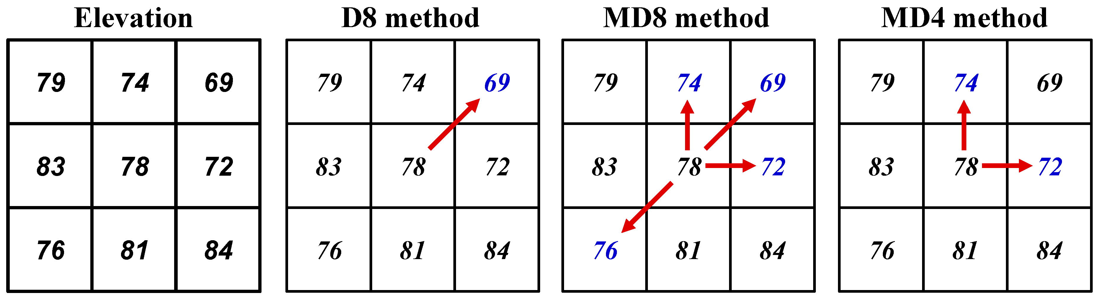
As shown in Figure 2, a schematic elevation dataset is provided for explaining flow-direction methods. Three types of methods were selected because they are the most widely applied and common for fully distributed runoff simulations. The rule of flow-direction determination based on the grid-based data can be broadly classified into two categories. One is the single-flow-direction (SFD) method, which routes the total mass of outflow from one grid to another following the steepest descent surrounded, called as eight-direction (D8) method [2,6,26]. The other one is the multiple-flow-direction (MFD) method [3,4,5,7,25], which can deliver the flow mass from one grid to multiple adjacent grids in order to perform a comparatively dispersive nature of surface runoff. The principles of determining flow paths and partitioning flow using the MD8 and MD4 methods are respectively illustrated as follows:
3.1. MD8 Method
The MD8 method is the earliest multiple-flow-direction method proposed by Quinn et al. [3]. As shown in Figure 2, this method assigns the flow directions to all its neighboring grids which have lower elevations; the flow fraction appointed to each downstream receiving grid i is as follows:
in which m is the total number of directions which have a downward slope; Si is the ground slope between the central grid and an adjacent grid i; Li denotes the effective contour length of the ith direction. The contour length is calculated according to the assumption: the possible eight flow directions have a consistent angle between any two adjacent directions. Quinn et al. [3] clearly indicated that the contour length is 0.5 for the cardinal directions and 0.354 for the diagonal directions.
3.2. MD4 Method
The multiple-four-direction (MD4) method has been widely adopted in many distributed runoff models [27,28,29,30]. As shown in Figure 2, in this method, only the cardinal flow directions, respectively representing the directions of the x-axis and y-axis in a Cartesian coordinate system, are considered. The rule to calculate flow fractions can be analogized to the MD8 method as shown in Equation (1) but omitting the four diagonal flow directions, it can be given by
4. Hydrological Modeling Based on Different Flow-Direction Methods
The three flow-direction methods, D8, MD8 and MD4, expressed in Equations (1) and (2), were separately applied with the numerical scheme to perform rainfall-runoff simulations, the governing equations and numerical approaches are explained in this section.
4.1. Governing Equations
The distributed hydrological model for overland-flow routing is usually based on the Saint Venant equations which are composed by the continuity and momentum equations as follows:
in which h is the water depth; q is the discharge per unit width; ie is the intensity of excess rainfall; So is the ground slope; Sf is the friction slope. To achieve a more efficient and stable routing process, the diffusion-wave approximation has been widely applied for runoff simulation [22,31,32,33] to replace the full type of momentum equation shown in Equation (4), which requires more complicated mathematical operations. By neglecting the local and convective acceleration terms in Equation (4), the momentum equation can be expressed as
The discharge of overland flow at each grid can be derived by adopting Manning’s equation as follows:
where n is the Manning roughness coefficient. Since the analytical solution for this set of governing equations is unavailable, numerical schemes are necessary to be applied.
4.2. Numerical Scheme
Based on the concept of the first-order backward finite difference scheme, the continuity equation as shown in Equation (3) can be expressed as [22]
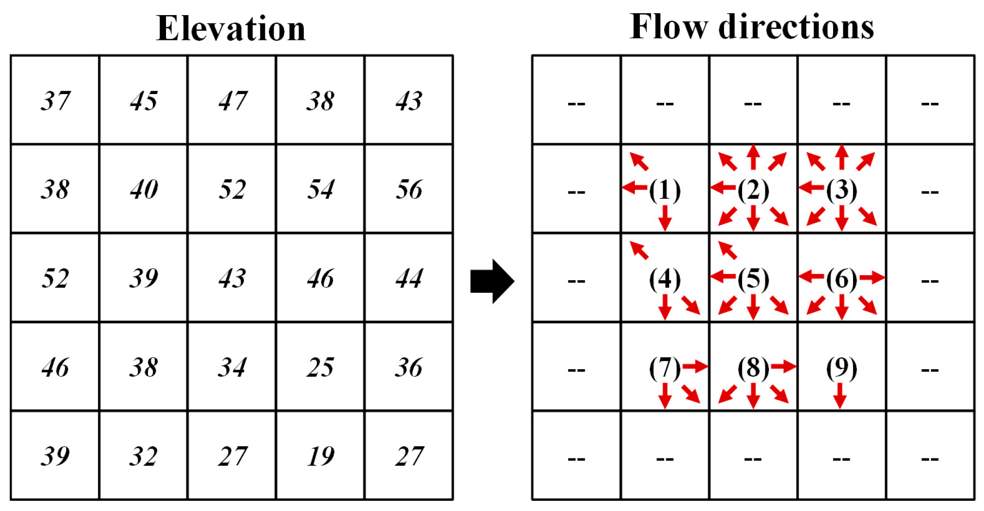
where is the total inflow discharge per unit width draining to the grid i, namely the accumulated discharge collected from upstream adjacent grids; denotes the total outflow discharge per unit width leaving from the grid i. For example, as shown in Figure 3, the total inflow discharge of No. 5 grid can be expressed as
and the total outflow discharge can be obtained by
where f is the flow fraction partitioned to the downstream receiving grids, which depends on the different rules of flow-direction methods mentioned above. After calculating the update water depth following Equation (7), the discharge of grid i at can be derived by applying the discretized momentum equation as follows:
where N is the number of downslope receiving grids leaving from the grid i. It should be noted that Equation (10) is also applicable to the single-flow-direction method (D8 method) as long as the N and f are assumed as 1.
5. Indexes for Evaluating Hydrograph Deviations
The drainage area of a watershed has been considered as a significant parameter used for a hydrological analysis and related design work; however, it can be very different because of diverse flow-direction assumptions applied for calculations and the variability of the terrain [10]. Huang and Lee [24] introduced two types of definitions for the extraction of the drainage area to illustrate the flow dispersion effects inherent in different flow-direction methods. The two types of drainage areas were regarded to explain the hydrograph shapes and hydrograph deviations among different flow-direction methods.
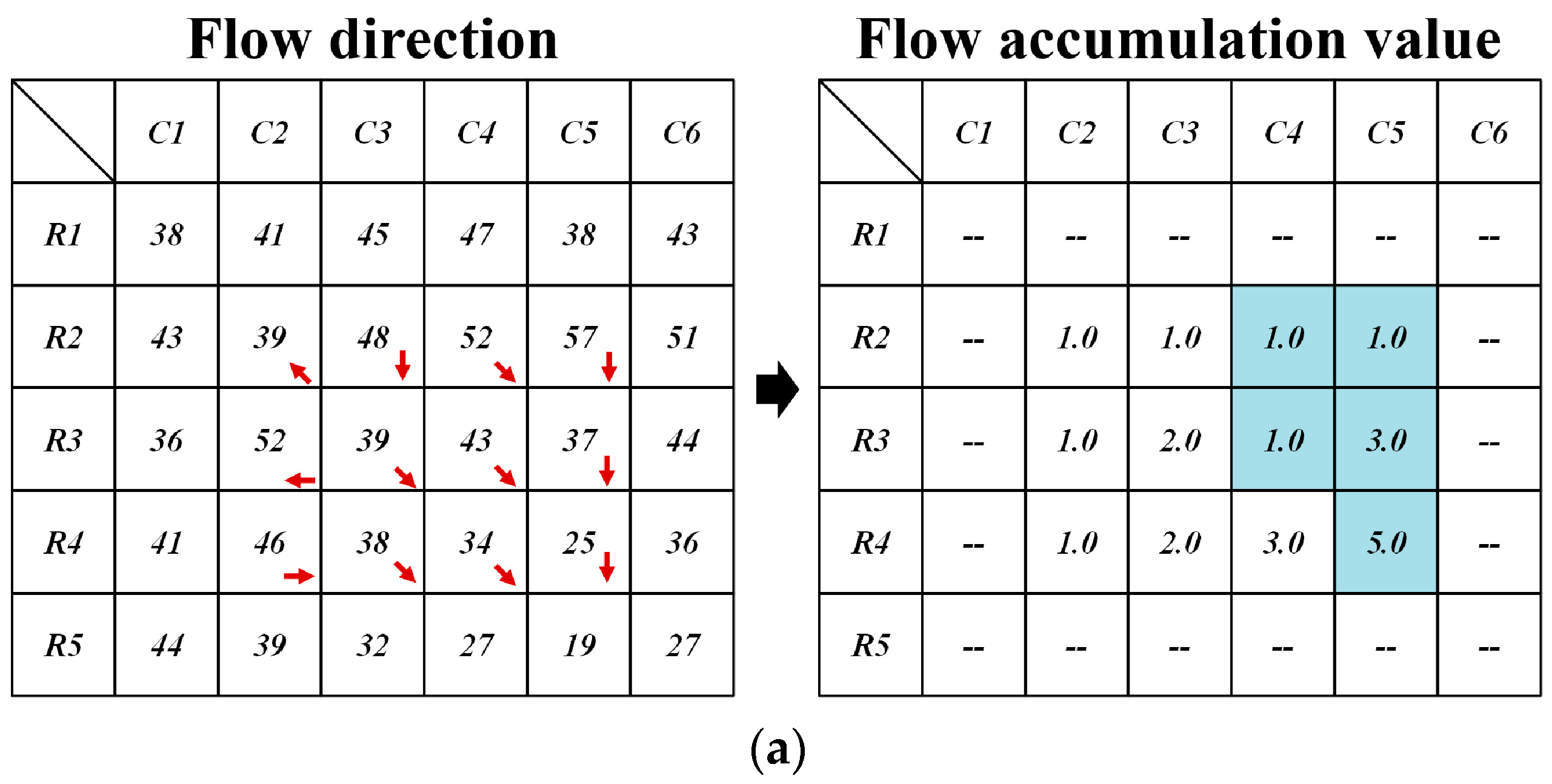
For example, Figure 4a shows a simple elevation dataset in which the elevation values are marked. According to the D8 method, the flow transferred from one grid to another follows the direction of steepest descent. When an outlet location is determined at R4C5, the whole drainage area, shaded in light blue color, can be delineated and it can be seen that a total of 5 grids are contained. This means that the flow accumulation value (FAV) at the watershed outlet is equal to the number of grids within the watershed boundary when the D8 algorithm is applied.
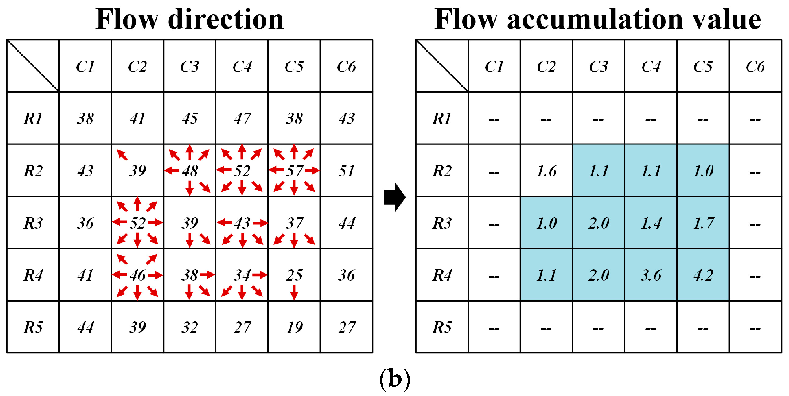
Relatively, as shown in Figure 4b, if the MD8 method is applied to the identical elevation dataset, the number of possible flow paths increases. The watershed extent, recognized by marking all the grids that can drain into the appointed outlet (at R4C5) through any possible flow path, is shaded in blue color; hence, it can be known that a total of 11 grids are included. The watershed extent extracted by this way is called the “flow dispersion area (AD)”, which denotes a maximum upstream extent that can affect the flow condition at the appointed outlet. Moreover, there is another index, called the “flow concentration area (AC)”, used to calculate the upstream contributing area as follows:
where (AC)i is the flow concentration area at grid i; a is the unit area of a grid; K is the total number of upstream grids connecting to grid i; FAVk is the flow accumulation value of grid k, which is one of the upstream adjacent grids connecting to grid i; fk is the flow fraction portioned from grid k to grid i. Different approaches to derive the flow fractions are explained in the previous section. In Figure 4b, the MD8 method is applied to calculate the flow fraction of each grid according to Equation (1). It can be seen that the flow concentration area at the outlet (R4C5) is equal to 4.2 grids, which is significantly less than the flow dispersion area (=11 grids). In brief, when applying the single-flow-direction (D8) method, the flow dispersion area is certainly equal to the flow concentration area; however, when adopting any type of multiple-flow-direction methods, the flow dispersion area is considered to be larger than the flow concentration area.
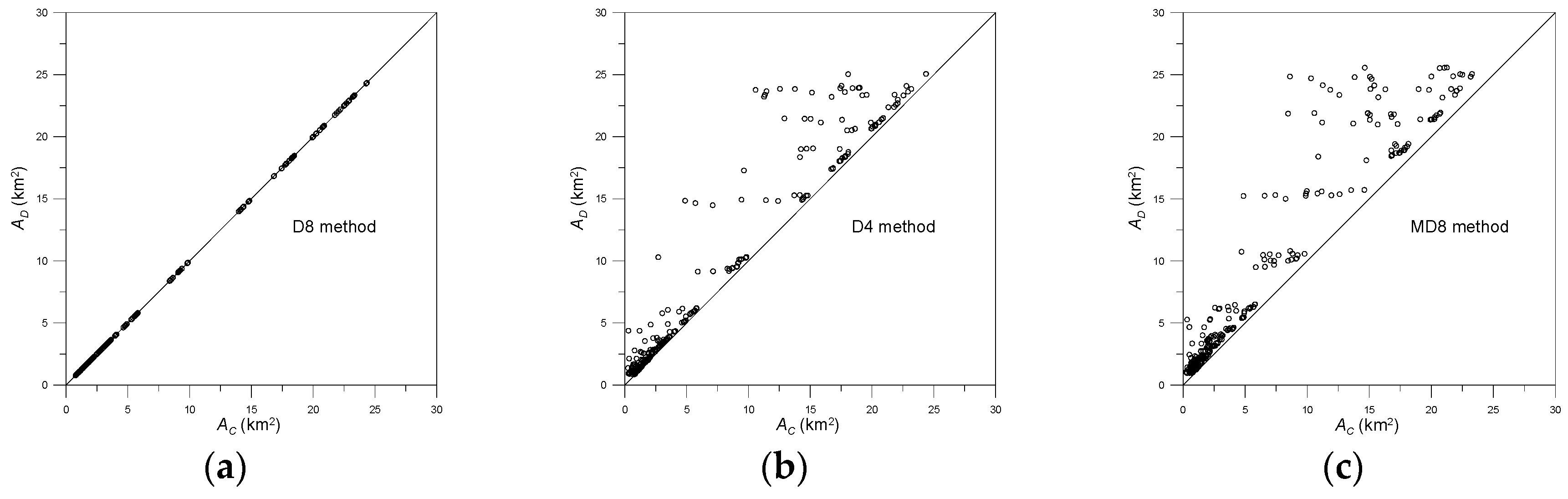
In this study, 300 locations in the Goodwin Creek Watershed were chosen to investigate the behaviors of simulated hydrographs using various flow-direction methods. The flow dispersion area AD and flow concentration area AC at each location calculated by adopting the D8, MD4 and MD8 methods are shown in Figure 5. It can be seen that when the MD4 or MD8 method is used to replace the D8 (single-flow-direction) method, the distribution of these points obviously shifts to the upper-left side of the diagonal line, showing the variance between the two types of drainage area. According to the results, it can be seen that a point which has a greater flow dispersion area (namely the total upstream area that can affect the flow response at a selected outlet) does not mean that it is able to collect a greater amount of outflow volume when a multiple-flow-direction method is adopted.
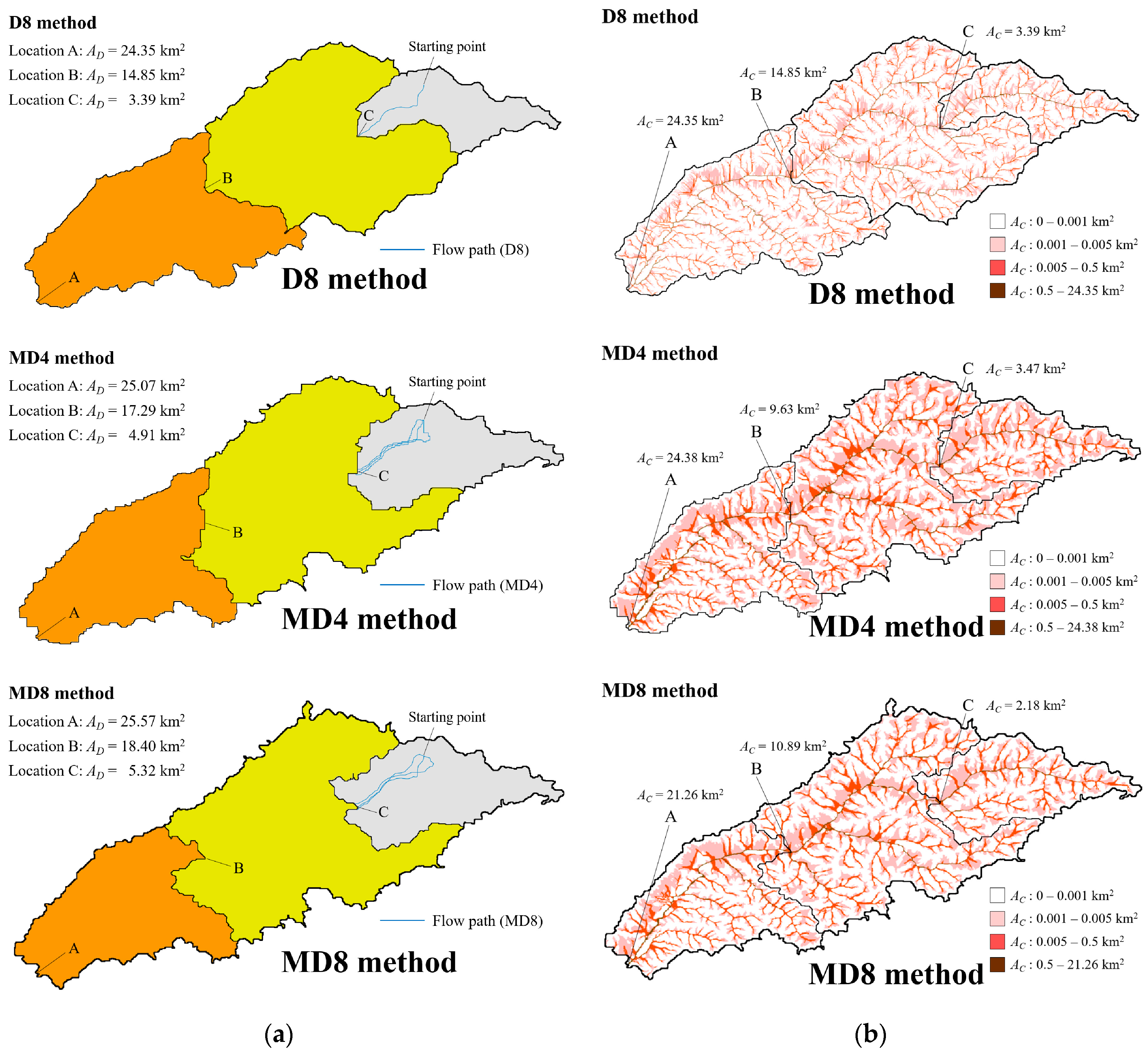
According to the definition of flow dispersion area (AD), the watershed boundaries for the three designated locations (as shown in Figure 1) can be determined using different FD methods and shown in Figure 6a. For the watershed outlet at location A, the largest watershed extent (AD) among the three FD methods is equal to 25.57 km2 when the MD8 method is applied. However, the MD8 method cannot guarantee collectnig the largest amount of flow volume due to its dispersion effect. For example, as shown in Figure 6a, the flow paths from a starting point in the upstream watershed are tracked individually using the D8, MD4 and MD8 methods. In fact, countless flow paths can occur when using MFD methods (MD4 or MD8) but only three of them are plotted to explain that there can be more than two outlet locations on the boundary grids to discharge the outflow. This causes the MFD method to be unable to collect a larger amount of water volume than the D8 method sometimes. In addition to checking the watershed boundary, the flow concentration area (AC) obtained from the flow accumulation value (FAV) was also investigated to evaluate the ability to collect flow volume for a designated point. The spatial distributions of flow concentration area (AC) are shown in Figure 6b using various FD methods. As revealed in these figures, the D8 method collects the largest value of AC at the outlet (location A), but the MFD methods can obtain a larger space with an AC greater than 0.005 km2.
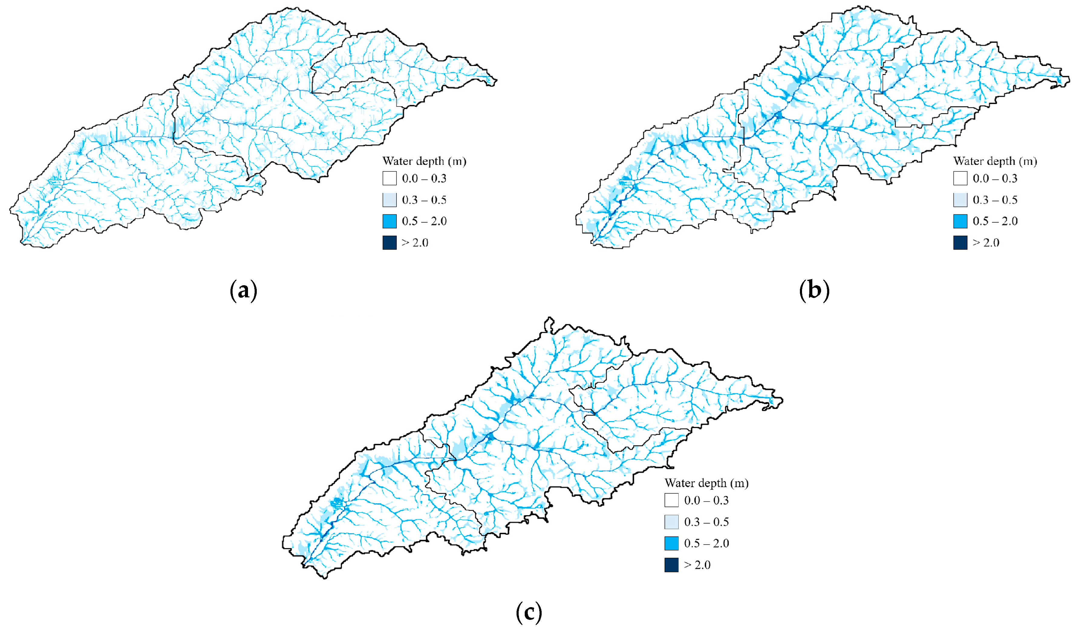
A rainfall condition with the constant intensity of 60 mm/h lasting for six hours was assigned to numerical runoff models for detecting the spatial distributions of water depth at the 10th hour of simulation using various FD methods, in the test the land surface is assumed as an impervious layer without any loss from infiltration. The maps of the simulated water depth at the 10th hour can be seen in Figure 7. The spatial distribution of water depth, showing the stream network, is similar to that of the flow concentration area (AC), as shown in Figure 6b. Therefore, it can be inferred that the flow concentration area (AC) can be an index to evaluate the ability to collect flow in the runoff simulation. The relation between the AC and the total outflow volume of hydrograph at each grid is worth analyzing. On the other hand, since AD also represents the upstream catchment area in which surface water can be retained or stored before it is drained out of the boundary, AD is assumed to be related to the runoff concentration time. In the following section, we intend to elaborate on how the two indexes, AC and AD, influence the features of a simulated hydrograph.
6. Hydrograph Deviations and Mass Conservation Test
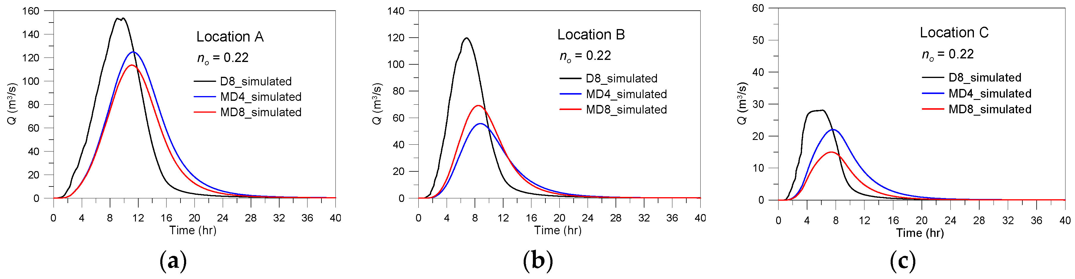
Three locations, marked as A, B, and C in the watershed, as shown in Figure 1, were selected to detect differences in the simulated hydrographs using various flow-direction methods. The rainfall condition assigned in the runoff models is the same as mentioned in the previous section. The discharge responses at the three locations can be seen in Figure 8. It can be found that the hydrograph using the MFD method (MD4 or MD8) does not present a consistent feature compared with that using the D8 method. For instance, both the MD4 and MD8 methods result in a significant loss in total outflow volume at location B, but this situation was not detected at the other two locations. In the aspect of flow peak, the MD4 method shows a greater peak discharge of the hydrograph than the MD8 method does at locations A and C, but such a result cannot be seen at location B. Therefore, this study intends to elaborate on how the flow-direction method causes these inconsistent behaviors in the simulated hydrographs.
A test of mass conservation wass also conducted to ensure that the total water volume received from the rainfall input does not loose during the process of simulation. Based on different flow-direction methods adopted in numerical models, Table 2 sequentially shows (1) the total volume of rainfall input within the watershed boundary whose outlet is at location B, (2) the sum of accumulated outflow volume (discharging from location B and all the grids on the watershed boundary) until the 10th hour, (3) total flow volume remaining in the watershed at the 10th hour (as shown in Figure 7). As listed in Table 2, the maximum relative error among the three cases applying various flow-direction methods is only 0.0087. This demonstrates that the total flow volume is conserved during the calculated process in executing the present numerical model based on various flow-direction methods.
7. Hydrograph Deviation Analyses
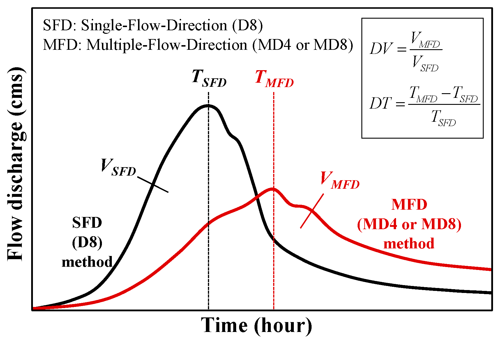
As explained in the previous section and Figure 8, the hydrograph shapes can be quite different because of th evarious flow-direction methods adopted in the model for runoff simulations. The two indexes, flow dispersion area and flow concentration area, have been found to vary with the flow-direction methods, therefore, they are assumed as two dominant factors to affect the hydrograph deviations between different flow-direction methods. Moreover, two aspects of hydrograph deviation, (1) the total volume of outflow discharge and (2) time to peak discharge, were concerned and aimed to be realized. Figure 9 shows a schematic diagram to illustrate the hydrograph deviations.
Compared to the simulated hydrograph which applies the D8 method, the two aspects of deviation between any one of MFD methods and the SFD (D8) method can be quantified and their relations with the two aforementioned indexes are expressed as follows:
where DV and DT are, respectively, the deviations of the total volume of outflow discharge and the time to peak discharge; VSFD and VMFD denote the outflow volumes separately, applying the SFD (D8) method and one of the MFD methods; TSFD and TMFD represent the time to flow peaks, separately, applying the SFD (D8) method and one of the MFD methods.
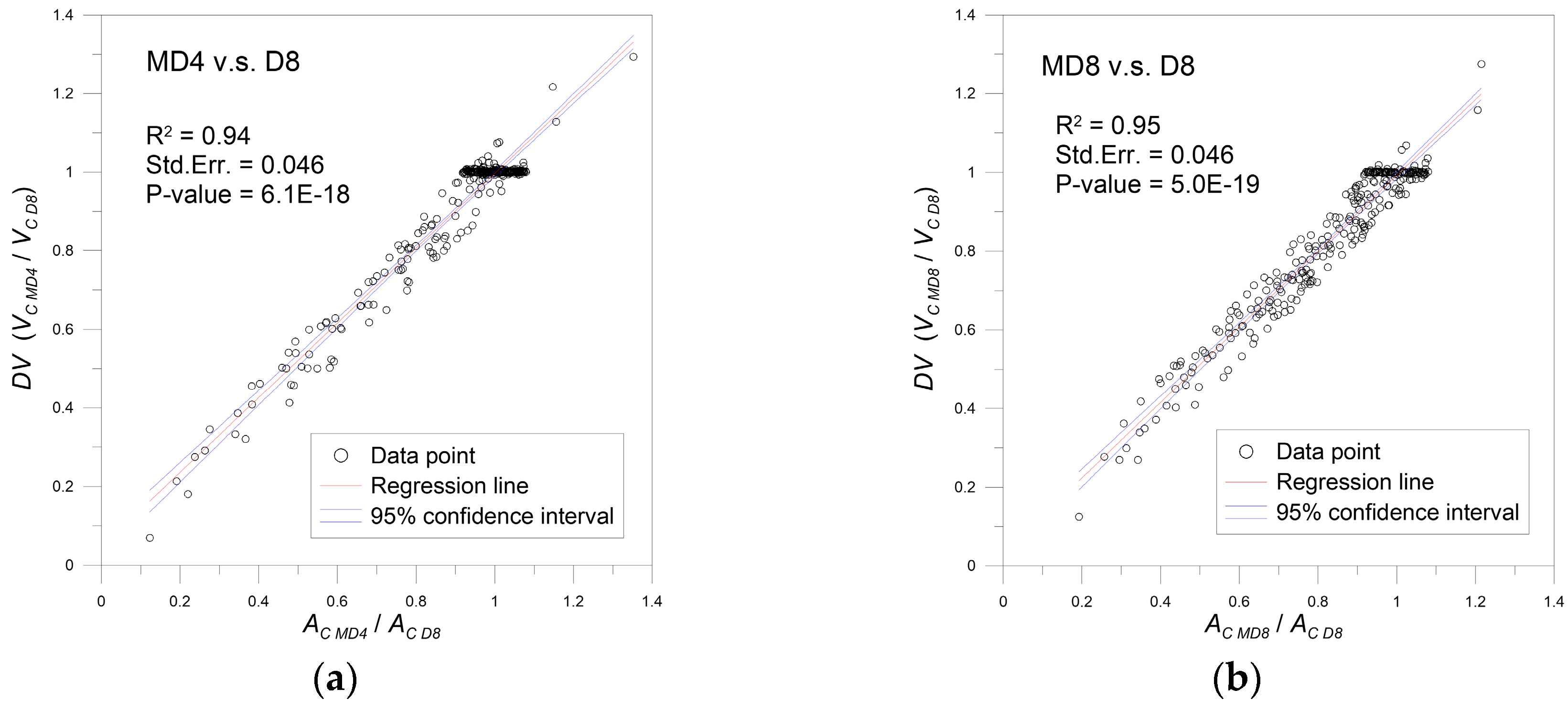
A series of rainfall-runoff simulations were conducted to evaluate the hydrograph deviations by using Equations (12) and (13). Rainfall events with a constant intensity of 10–60 mm/h lasting for 3–12 h were assigned to the three types of models. Simulated hydrographs at 300 locations in the Goodwin Creek Watershed were collected for analyses. The accumulated area under each discharge hydrograph was calculated to obtain the total volume of outflow; therefore, the relation between the DV and ratio of AC at each location can be plotted in Figure 10 based on the MD4 and MD8 methods comparing to the D8 method.
Both figures show that the magnitude of DV is quite relevant to the ratio of AC. A linear regression model was conducted to estimate the two regression functions as follows:
The above results of the linear regression analysis can be expressed as the two trend lines plotted in Figure 10, in which the 95% confidence interval of the regression model was also provided. A statistical measure, R2 coefficient of determination, was adopted to indicate how well the regression line approximates the observed data points. The R2 coefficient is given by
where d is the total number of observed data, is the observed deviation (DV or DT), is the mean of the observed deviations, and is the predicted deviation using a regression model. The results show that the R2 coefficient is equal to 0.9483 when the MD4 method is compared with the D8 method; this can be interpreted in that 94.83 percent of the variance in the DV can be explained by the variable (ratio of AC). The R2 coefficient equals to 0.9463 when the MD8 method is compared with the D8 method. Overall, for the two sets of analyses, the R2 values demonstrate the good fitness of the regression model.
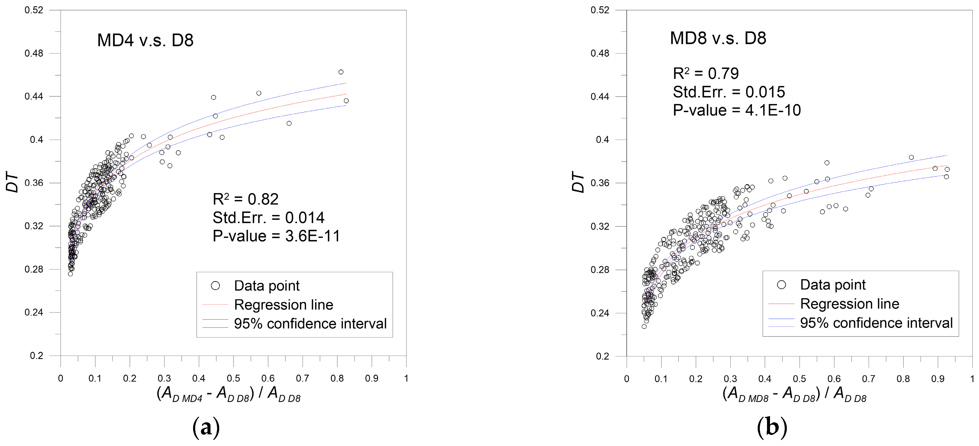
Likewise, following the same method to analyze the deviation of time to flow peak (DT), the results for the 300 survey locations can be seen in Figure 11 based on the MD4 and MD8 methods comparing to the D8 method.
It can be found that the distribution of the data points can be approximately described by a natural logarithm function through the regression analysis with a 95% confidence interval. As shown in Figure 11, the deviation of time to flow peak (DT) basically increases with the variance of flow dispersion area (AD) between an MFD (MD4 or MD8) method and the D8 method, but the increment of DT gradually slows down. Moreover, as shown in Figure 11, the comparison of hydrographs between the MD4 and D8 methods shows greater values of DT than that between the MD8 and D8 methods. These two regression functions plotted in Figure 11 can be expressed as follows:
The R2 coefficients for the above two regression equations are 0.817 and 0.7943 respectively, this demonstrates that approximately 80 percent of DT can be described by the variance of flow dispersion area (AD) according to these two regression models shown in Equations (17) and (18).
8. Hydrograph Transformation from SFD Method to MFD Method
The previous section indicates that the hydrograph differences among various flow-direction methods depend on the variances of the flow concentration area (AC) and flow dispersion area (AD), and establishes the relations between the area indexes and the two types of deviations (DV and DT) by using regression models. According to the aforementioned results, this section intends to estimate the outflow discharge, analogously to the hydrograph by applying an MFD method from a simulated hydrograph that uses a numerical runoff model based on the SFD (D8) method.
8.1. Methodology
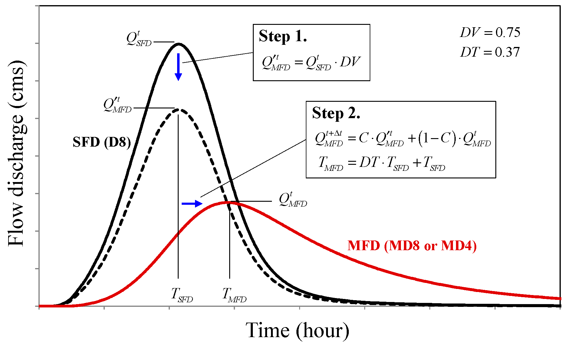
Two steps of calculation are proposed to adjust the simulated hydrograph separately in the aspects of total flow volume and time to peak discharge, as follows:
• Step 1. Adjustment of total flow volume
The deviation of total outflow volume (DV) is first adopted to calculate the total flow mass of discharge hydrograph as follows:
where represents the simulated discharge generated by a runoff model by applying the SFD (D8) method; DV can be obtained from the linear regression models, as shown in Equations (14) and (15). The adjusted discharge hydrograph, denoted as , is illustrated in Figure 12.
• Step 2. Adjustment of time to peak discharge
In order to predict the discharge hydrograph which uses an MFD method, both considerations, (1) the shift of time to peak discharge and (2) the attenuation of flow peak, are required. Therefore, the discharge hydrograph obtained from Equation (19) is subsequently substituted into the following formulation to perform these situations,
where represents the estimated discharge analogous to that applying an MFD method at time t; C is a coefficient ranging from 0 to 1 and it can be determined by an iteration method. The optimal coefficient C corresponds to a discharge response whose time to flow peak is equal to
in which DT can be obtained from the natural logarithmic regression models as shown in Equations (17) and (18), and the time to flow peak using the D8 method (TSFD) is a known value. This step of adjustment can also be seen in the schematic diagram shown in Figure 12.
8.2. Simulation Results and Discussion
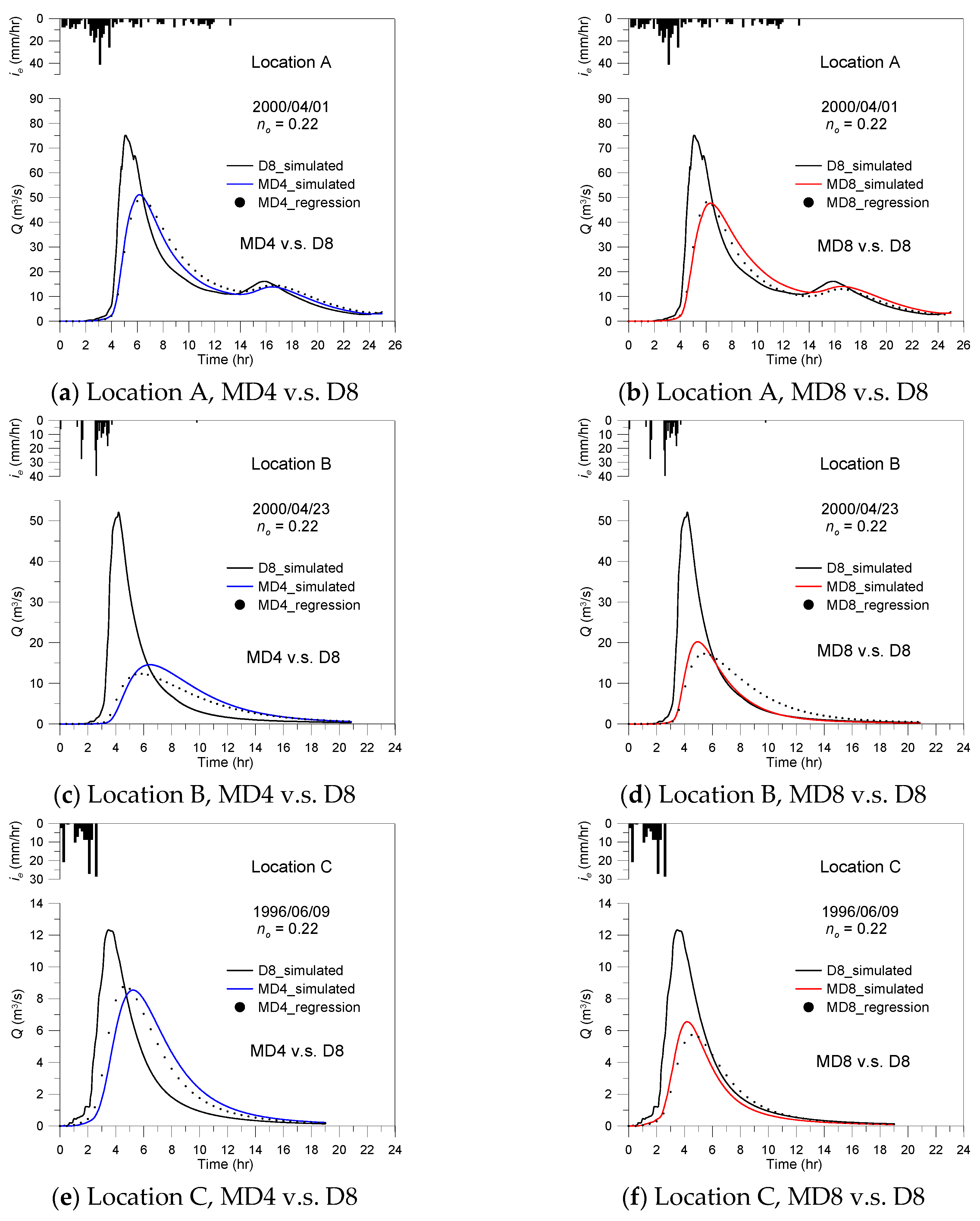
As shown in Table 2, the two area indexes (AC and AD) and the estimated deviations (DV and DT) of the three locations marked in Figure 1 are listed. Obvious variances of AC and AD between the D8 method and the MFD methods can be detected in this table; these two area indexes are subsequently adopted to estimate the hydrograph deviations by applying the regression models shown in Equations (14), (15), (17), and (18). The rainfall conditions of the three events were collected and assigned to the distributed runoff model separately using the D8, MD4 and MD8 methods.
The simulated discharge hydrographs, which apply different flow-direction methods at the three locations can be seen in Figure 13. The two types of estimated hydrograph deviations (DV and DT) listed in Table 3 were used to imitate the hydrograph shape of an MFD method by adjusting the flow discharge generated from the D8 runoff model by following the aforementioned procedure. The results of implementing the two steps of adjustment with the use of regression models are also provided in Figure 13.
Figure 13 shows that for each of the three locations, the total flow volume and the shape of simulated hydrographs by conducting MFD runoff models can generally be described by the proposed method based on the regression functions. This demonsrtates that the differences of simulated hydrographs among various flow-direction methods mainly depend on the variances of the flow dispersion area (AD) and flow concentration area (AC) at each location, in which the AC dominates the total volume of outflow and AD affects the time to peak discharge. A flow-direction method adopted in a runoff model does not directly indicate a unique feature in the hydrograph such as a higher peak discharge or a greater flow volume, but overall, the MFD methods can lead to a later time to reach flow peak and a smaller value of peak discharge compared to the SFD (D8) method. The research results also show that the hydrograph deviations among different flow-direction methods can be quantified by only extracting the two area indexes before an MFD method is selected for distributed runoff routing.
9. Conclusions
This study aimed to investigate the distinctions of simulated hydrographs affected by applying different flow-direction methods in the hydrological model. Considering that two types of geomorphological indexes, the flow concentration area (AC) and the flow dispersion area (AD), were found to be dependent on the flow-direction method, they were adopted as the factors to detect the deviations of simulated hydrographs in the aspects of water collecting capability and the time to peak discharge. Three types of flow-direction methods were applied to the digital elevation dataset of the Goodwin Creek watershed in the US for a series of rainfall-runoff simulations. The experimental results of 300 selected locations showed that the deviation of total outflow volume (DV) between two hydrographs using various flow-direction methods is highly relevant to the ratio of flow concentration area and can be well described by a linear regression function; the deviation of time to peak discharge (DT) is then dominated by the variance of flow dispersion area between two different flow-direction methods and can be approximated by a logarithmic regression function.
Moreover, a two-step adjustment for discharge hydrograph in terms of outflow volume and time to flow peak was proposed to imitate the profile of hydrograph generated from an MFD runoff model. Basically, the results of several rainfall events demonstrate that the simulated discharge hydrographs using MFD methods can be imitated by the proposed transformation approach based on the two deviations calculated from the regression models. These research findings manifest that merely the two area indexes (AC and AD) are capable of estimating the differences of simulated hydrographs between various flow-direction methods. Overall, compared to the SFD (D8) method, the MFD methods usually result in the delay of time to flow peak and less amount of total outflow volume.
Funding
This research received no external funding.
Acknowledgments
Financial support provided by the Ministry of Science and Technology, Taiwan under grant MOST 108-2625-M-019-004 is sincerely acknowledged.
Conflicts of Interest
The authors declare no conflict of interest.
References
- Douglas, D.H. Experiments to locate ridges and channels to create a new type of digital elevation model. Cartographica 1986, 23, 29–61. [Google Scholar] [CrossRef]
- Orlandini, S.; Moretti, G.; Franchini, M.; Aldighieri, B.; Testa, B. Path-based methods for the determination of nondispersive drainage directions in grid-based digital elevation models. Water Resour. Res. 2003, 39. [Google Scholar] [CrossRef] [Green Version]
- Quinn, P.; Beven, K.; Chevallier, P.; Planchon, O. The prediction of hillslope flow paths for distributed hydrological modelling using digital terrain models. Hydrol. Process. 1991, 5, 59–79. [Google Scholar] [CrossRef]
- Seibert, J.; McGlynn, B.L. A new triangular multiple flow direction algorithm for computing upslope areas from gridded digital elevation models. Water Resour. Res. 2007, 43. [Google Scholar] [CrossRef] [Green Version]
- Tarboton, D.G. A new method for the determination of flow directions and slope areas in grid digital elevation models. Water Resour. Res. 1997, 33, 309–319. [Google Scholar] [CrossRef] [Green Version]
- O’Callaghan, J.F.; Mark, D.M. The extraction of drainage networks from digital elevation data. Comput. Vis. Graph. Image Process. 1984, 28, 323–344. [Google Scholar] [CrossRef]
- Freeman, T.G. Calculating catchment area with divergent flow based on a regular grid. Comput. Geosci. 1991, 17, 413–422. [Google Scholar] [CrossRef]
- Galland, J.C.; Goutal, N.; Hervouet, J.-M. TELEMAC: A new numerical model for solving shallow water equations. Adv. Water Resour. 1991, 14, 138–148. [Google Scholar] [CrossRef]
- Zhou, Q.; Liu, X.; Sun, Y. Terrain complexity and uncertainties in grid-based digital terrain analysis. Int. J. Geogr. Inf. Sci. 2006, 20, 1137–1147. [Google Scholar] [CrossRef]
- Erskine, R.H.; Green, T.R.; Ramirez, J.A.; MacDonald, L.H. Comparison of grid-based algorithms for computing upslope contributing area. Water Resour. Res. 2006, 42. [Google Scholar] [CrossRef] [Green Version]
- Pilesjö, P. An integrated raster-TIN surface flow algorithm. In Advances in Digital Terrain Analysis; Springer: Berlin/Heidelberg, Germany, 2008; pp. 237–255. [Google Scholar]
- Pilesjö, P.; Hasan, A. A triangular form-based multiple flow algorithm to estimate overland flow distribution and accumulation on a digital elevation model. Trans. GIS 2014, 18, 108–124. [Google Scholar] [CrossRef] [Green Version]
- Aryal, S.K.; Bates, B.C. Effects of catchment discretization on topographic index distributions. J. Hydrol. 2008, 359, 150–163. [Google Scholar] [CrossRef]
- Beven, K.J.; Kirkby, M.J. A physically based variable contributing area model of basin hydrology. Hydrol. Sci. J. 1979, 24, 43–69. [Google Scholar] [CrossRef] [Green Version]
- Beven, K.J.; Wood, E.F. Catchment geomorphology and the dynamics of runoff contributing areas. J. Hydrol. 1983, 65, 139–158. [Google Scholar] [CrossRef]
- Kumar, R.; Chatterjee, C.; Singh, R.D.; Lohani, A.K.; Kumar, S. Runoff estimation for an ungauged catchment using geomorphological instantaneous unit hydrograph (GIUH) models. Hydrol. Process. 2007, 21. [Google Scholar] [CrossRef]
- Lee, K.T.; Yen, B.C. Geomorphology and Kinematic-Wave–Based Hydrograph Derivation. J. Hydraul. Eng. 1997, 123, 73–80. [Google Scholar] [CrossRef]
- Lee, K.T.; Chang, C.-H. Incorporating subsurface-flow mechanism into geomorphology-based IUH modeling. J. Hydrol. 2005, 311, 91–105. [Google Scholar] [CrossRef]
- O’Loughlin, E.M. Prediction of surface saturation zones in natural catchments by topographic analysis. Water Resour. Res. 1986, 22, 794–804. [Google Scholar] [CrossRef]
- Pan, F.; Peters-Lidard, C.D.; Sale, M.J.; King, A.W. A comparison of geographical information systems–based algorithms for computing the TOPMODEL topographic index. Water Resour. Res. 2004, 40. [Google Scholar] [CrossRef] [Green Version]
- Rodriguez-Iturbe, I.; Gonzalez-Sanabria, M.; Bras, R.L. The Geomorphoclimatic theory of the instantaneous unit hydrograph. Water Resour. Res. 1982, 18, 877–886. [Google Scholar] [CrossRef]
- Wang, M.; Hjelmfelt, A.T. DEM based overland flow routing modeling. J. Hydrol. Eng. 1998, 3, 1–8. [Google Scholar] [CrossRef]
- Wolock, D.W.; McCabe, G.J., Jr. Comparison of single and multiple flow direction algorithms for computing topographic parameters in TOPMODEL. Water Resour. Res. 1995, 31, 1315–1324. [Google Scholar] [CrossRef]
- Huang, P.-C.; Lee, K.T. Distinctions of geomorphologic properties caused by different flow-direction predictions from digital elevation models. Int. J. Geogr. Inf. Sci. 2016, 30, 168–185. [Google Scholar] [CrossRef]
- Lindsay, J.B. A physically based model for calculating contributing area on hillslopes and along valley bottoms. Water Resour. Res. 2003, 39. [Google Scholar] [CrossRef]
- Jenson, S.K.; Domingue, J.O. Extracting topographic structure from digital elevation data for geographic information system analysis. Photogramm. Eng. Remote Sens. 1988, 54, 1593–1600. [Google Scholar]
- Bates, P.D.; De Roo, A.P.J. A simple raster-based model for flood inundation simulation. J. Hydrol. 2000, 236, 54–77. [Google Scholar] [CrossRef]
- Gallant, J.C.; Hutchinson, M.F. A differential equation for specific catchment area. Water Resour. Res. 2011, 47. [Google Scholar] [CrossRef] [Green Version]
- Maksimovic, C.; Prodanovic, D.; Boonya-aroonnet, S.; Leitao, J.P.; Djordjevic, S.; Allitt, R. Overland flow and pathway analysis for modelling of urban pluvial flooding. J. Hydraul. Res. 2009, 47, 512–523. [Google Scholar] [CrossRef]
- O’Brien, J.S.; Julien, P.Y.; Fullerton, W.T. Two-dimensional water flood and mudflow simulation. J. Hydraul. Eng. 1993, 119, 244–261. [Google Scholar] [CrossRef]
- Gonwa, W.S.; Kavvas, M.L. A modified diffusion wave equation for flood propagation in trapezoidal channels. J. Hydrol. 1986, 83, 119–136. [Google Scholar] [CrossRef]
- Jain, M.K.; Singh, V.P. DEM-based modeling of surface runoff using diffusion wave equation. J. Hydrol. 2005, 302, 107–126. [Google Scholar] [CrossRef]
- Ogden, F.L.; Julien, P.Y. Runoff sensitivity to temporal and spatial rainfall variability at runoff plane and small basin scales. Water Resour. Res. 1993, 29, 2589–2597. [Google Scholar] [CrossRef]
Figure 1.
Geographical location and topography of the Goodwin Creek watershed.

Figure 2.
Comparison of different methods of flow-direction determination.

Figure 3.
Flow-direction assignation using the MD8 method.

Figure 4.
Calculations of two area indexes based on different flow-direction methods: (a) D8 method; (b) MD8 method.
Figure 4.
Calculations of two area indexes based on different flow-direction methods: (a) D8 method; (b) MD8 method.


Figure 5.
Variances between the flow dispersion area and the flow concentration area at the 300 locations using three selected flow-direction methods: (a) D8 method; (b) MD4 method; (c) MD8 method.
Figure 5.
Variances between the flow dispersion area and the flow concentration area at the 300 locations using three selected flow-direction methods: (a) D8 method; (b) MD4 method; (c) MD8 method.

Figure 6.
Comparison of area indexes using different flow-direction methods: (a) Flow dispersion areas of three designated outlets; (b) Distributions of flow concentration areas.
Figure 6.
Comparison of area indexes using different flow-direction methods: (a) Flow dispersion areas of three designated outlets; (b) Distributions of flow concentration areas.

Figure 7.
Comparison of water-depth distribution using different flow-direction methods: (a) D8 method; (b) MD4 method; (c) MD8 method.
Figure 7.
Comparison of water-depth distribution using different flow-direction methods: (a) D8 method; (b) MD4 method; (c) MD8 method.

Figure 8.
Simulated hydrographs based on different flow-direction methods at the three locations in the watershed: (a) Location A; (b) Location B; (c) Location C.
Figure 8.
Simulated hydrographs based on different flow-direction methods at the three locations in the watershed: (a) Location A; (b) Location B; (c) Location C.

Figure 9.
Indicators of hydrograph deviations between the D8 method and an MFD method.

Figure 10.
Relationship between the flow-volume deviation (DV) and the ratio of flow concentration area: (a) MD4 compared to D8; (b) MD8 compared to D8.
Figure 10.
Relationship between the flow-volume deviation (DV) and the ratio of flow concentration area: (a) MD4 compared to D8; (b) MD8 compared to D8.

Figure 11.
Relationship between the peak-time deviation (DT) and the variance of flow dispersion area: (a) MD4 compared to D8; (b) MD8 compared to D8.
Figure 11.
Relationship between the peak-time deviation (DT) and the variance of flow dispersion area: (a) MD4 compared to D8; (b) MD8 compared to D8.

Figure 12.
Flow discharge transformation analogizing to the hydrograph shape generated from an MFD runoff model.
Figure 12.
Flow discharge transformation analogizing to the hydrograph shape generated from an MFD runoff model.

Figure 13.
Comparisons of discharge hydrographs generated from the distributed runoff model and the regression model at three designated outlets.
Figure 13.
Comparisons of discharge hydrographs generated from the distributed runoff model and the regression model at three designated outlets.


Table 1.
Geomorphological conditions of the Goodwin Creek watershed.
| Drainage Area | Altitude | Average Channel Slope | Landuse | Outlet Coordinates |
|---|---|---|---|---|
| 21.3 km2 | 71 m–128 m | 0.004 m/m | pasture & forest | 34.25° North 89.87° West |
Table 2.
Mass conservation test based on different flow-direction methods.
| Flow Direction Method | (1) | (2) | (3) | |(2) + (3) − (1)|/(1) |
|---|---|---|---|---|
| Total Volume of Rainfall Input (m3) | Accumulated Outflow Volume (m3) | Flow Volume Remaining in the Watershed (m3) | Relative Error | |
| D8 | 5344812 | 3960309 | 1338003 | 0.0087 |
| MD4 | 6223140 | 4193925 | 1996855 | 0.0052 |
| MD8 | 6624684 | 4576201 | 2001448 | 0.0071 |
Note: Total volume of rainfall input = AD × ie × rainfall duration;
Accumulated outflow volume = total flow volume discharging from location B and watershed boundary.
Table 3.
Area indexes and estimated hydrography deviations (DV and DT) at the three locations in the Goodwin Creek Watershed.
Table 3.
Area indexes and estimated hydrography deviations (DV and DT) at the three locations in the Goodwin Creek Watershed.
| Location | FD Method | Area Index (km2) | Regression Function | ||
|---|---|---|---|---|---|
| AC | AD | DV | DT | ||
| A | MD4 | 24.38 | 25.07 | 0.999 | 0.297 |
| MD8 | 21.26 | 25.57 | 0.874 | 0.254 | |
| D8 | 24.35 | 24.35 | -- | -- | |
| B | MD4 | 9.63 | 17.29 | 0.649 | 0.372 |
| MD8 | 10.89 | 18.40 | 0.736 | 0.320 | |
| D8 | 14.85 | 14.85 | -- | -- | |
| C | MD4 | 3.47 | 4.91 | 1.021 | 0.416 |
| MD8 | 2.18 | 5.32 | 0.647 | 0.356 | |
| D8 | 3.39 | 3.39 | -- | -- | |
© 2020 by the author. Licensee MDPI, Basel, Switzerland. This article is an open access article distributed under the terms and conditions of the Creative Commons Attribution (CC BY) license (http://creativecommons.org/licenses/by/4.0/).
Share and Cite
MDPI and ACS Style
Huang, P.-C. Analysis of Hydrograph Shape Affected by Flow-Direction Assumptions in Rainfall-Runoff Models. Water 2020, 12, 452. https://doi.org/10.3390/w12020452
AMA Style
Huang P-C. Analysis of Hydrograph Shape Affected by Flow-Direction Assumptions in Rainfall-Runoff Models. Water. 2020; 12(2):452. https://doi.org/10.3390/w12020452
Chicago/Turabian StyleHuang, Pin-Chun. 2020. "Analysis of Hydrograph Shape Affected by Flow-Direction Assumptions in Rainfall-Runoff Models" Water 12, no. 2: 452. https://doi.org/10.3390/w12020452
Note that from the first issue of 2016, this journal uses article numbers instead of page numbers. See further details here.