Numerical and Experimental Investigation of Wave Overtopping of Barriers
by
 ,
,
Giovanni Cannata
1,* ,
,
Marco Tamburrino
1,
Simone Ferrari
2,
Maria Grazia Badas
2 and
Giorgio Querzoli
2 1
Department of Civil, Constructional and Environmental Engineering, “Sapienza” University of Rome, Via Eudossiana 18, 00184 Roma (RM), Italy
2
Department of Civil and Environmental Engineering and Architecture, University of Cagliari, Via Marengo 2, 09123 Cagliari (CA), Italy
*
Author to whom correspondence should be addressed.
Water 2020, 12(2), 451; https://doi.org/10.3390/w12020451
Submission received: 3 December 2019
/
Revised: 16 January 2020
/
Accepted: 29 January 2020
/
Published: 8 February 2020
(This article belongs to the Special Issue Numerical Modelling of Wave Fields and Currents in Coastal Area)
Abstract
:We present a study of wave overtopping of barriers. The phenomenon of the wave overtopping over emerged structures is reproduced both numerically and experimentally. The numerical simulations are carried out by a numerical scheme for three-dimensional free-surface flows, which is based on the solution of the Navier–Stokes equations in a novel integral form on a time-dependent coordinate system. In the adopted numerical scheme, a novel wet–dry technique, based on the exact solution of the Riemann problem over the dry bed, is proposed. The experimental tests are carried out by adopting a nonintrusive and continuous-in-space image-analysis technique, which is able to properly identify the free surface even in very shallow waters or breaking waves. A comparison between numerical and experimental results, for several wave and water-depth conditions, is shown.
1. Introduction
The prediction of the wave overtopping process over barriers is fundamental to properly design seawalls, breakwaters, sea dikes and, more generally, structures that have the aim to protect inland areas from sea waves. For this reason, a large number of studies (e.g., [1,2,3,4,5]) has been carried out in the past years with the aim of giving estimation to the fundamental parameters that govern the aforementioned phenomenon. These studies led to the development of modern overtopping prediction formulae [6]. This approach provides a method of evaluation of several essential parameters (overtopping discharge, maximum run-up, wave transmission), being a robust and simple tool for the prediction of the key aspects of wave overtopping.
An alternative strategy to study the wave overtopping phenomenon consists in the use of numerical models. In order to have a reliable prediction of the wave overtopping over a structure, a numerical model has to consistently simulate different phenomena: wave transformation from deep to shallow water, wave breaking over variable bathymetry, wave run-up on the structure, wave transmission, three-dimensional effects. The first numerical models presented in literature for the overtopping simulation were based on solution of the depth-averaged Nonlinear Shallow Water Equations (NSWE) (e.g., [7,8,9]). Using shock-capturing methods, these NSWE-type models possess the capability to naturally simulate wave breaking [8]. Unfortunately, in NSWE models, frequency dispersion effects are neglected, so wave propagation cannot be properly reproduced. To overcome this issue, a number of models were created solving depth-averaged Boussinesq Equations (e.g., [10,11,12]), which incorporate nonlinear and dispersive properties. Boussinesq-type models are able to simulate both wave propagation (thanks to the modeling of the dispersive terms) and wave breaking (thanks to the shock-capturing property); for this reason, in recent years they were widely used for wave overtopping studies [13]. The drawback of these models is that in the shallow water zones, to properly simulate wave transformation and breaking, dispersive terms have to be turned off, essentially switching from Boussinesq Equations to NSWE, so that these models are not completely parameter free; in fact, a criterion to define the switch zone from one set of equations to the other one, has to be chosen.
The limiting aspects of depth-averaged type models can be encompassed by using a model that solves the three-dimensional Navier–Stokes (NS) Equations [14,15,16]. In the early NS-type models, the hydrostatic pressure assumption is made (i.e., [17]). When the vertical fluid acceleration is strong, mostly in presence of highly dispersive and nonlinear phenomena in deep and intermediate water, these models may be inaccurate. More recent models take into account the dynamic pressure. In such models, a two-step procedure is developed: in the first step, the NS equations are solved with the hydrostatic pressure assumption, neglecting the dynamic pressure; in the second step, the dynamic pressure is taken into account by solving the so-called Poisson equation.
Free-surface tracking is one of the most challenging issues in three-dimensional models for free-surface flows. Previous research [18,19] used the Volume Of Fluid (VOF) technique to locate free surface in a model in which the NS equations are numerically integrated in Cartesian coordinates. This technique is widely used in numerical methods for free-surface flows, being adopted in some of the most popular numerical codes available in literature (see for example, [20,21] for the application of the VOF technique to OpenFOAM®). By means of this technique, the vertical fluxes cross the computational cell arbitrarily. The drawback of this method is that a correct assignment of pressure and kinematic boundary conditions at the free surface is difficult. In a different class of models [22,23], in order to overcome the aforementioned drawback, the Navier–Stokes equations are expressed in a coordinate system in which the horizontal coordinates are the Cartesian coordinates and the vertical one is a time-varying coordinate that adjusts to the free-surface movements. By this strategy, the time-varying physical domain is mapped into a fixed rectangular-prismatic-shape computational grid, by means of a time-dependent vertical coordinate transformation; the free-surface position is at the upper computational boundary, so that the kinematic and zero-pressure conditions at the free surface can be assigned precisely. One of the main drawbacks of the aforementioned models is that they are not designed to explicitly simulate the wave breaking. In order to overcome this drawback, several authors recently proposed numerical models based on a conservative differential form [24] or on an integral form [25,26] of the Navier–Stokes equations, expressed in a time-dependent vertical coordinate system. In these models, the motion equations are numerically integrated by means of shock-capturing schemes. As opposed to Boussinesq-type models, no criterion has to be chosen to simulate wave-breaking phenomenon.
In the numerical models by [15], [25,26], a simple technique proposed by Ma et al. [24] is implemented in order to treat the wet–dry front movement: the criterion by means of which a dry cell changes its status to wet is based on a comparison with the free-surface elevation of the neighboring cells. This technique proved to be successful in cases in which there is a positive sloping bottom, but fail to predict the wet–dry front movement over emerged obstacles with flat or negative slope bottoms. In order to overcome this limitation and to extend the applicability of the model by [26] to the simulation of wave overtopping of barriers, in this work we propose a novel wet–dry technique, which is able to locate the wet–dry wave front over flat or negative slope bottoms. In the proposed wet–dry technique, the exact solution of the Riemann problem over dry bed is adopted to evaluate the celerity of the wet–dry wave front. This novel wet–dry technique is applied to the numerical model proposed by [26], and it is validated by numerically simulating the wave overtopping over barriers with flat crest and negative slope bottom and by comparing the numerical results with experimental data.
A set of experiments used to validate the numerical results, has been carried out in the wave flume of the Hydraulics Laboratory of the Department of Civil and Environmental Engineering and Architecture, University of Cagliari, Italy. Field [27] and laboratory measurements are widely used to validate numerical models [28,29]. Many of these measurements are carried out by means of resistive probes as experimental instruments, by means of which water level can be measured. Using resistive probes, the prediction of the water level in very shallow water zones and in the wave-breaking zone, is a challenging issue. In this context, Lorke et al. [3] used thin gauges and micropropellers to predict the water level and flow velocity at the crest of the structure. In order to overcome the aforementioned issue, we developed a nonintrusive and continuous-in-space technique, based on Image Analysis, developed and tested by Ferrari et al. [30]. This technique is able to properly identify the wave free surface even in prohibitive situations for traditional resistive probes, such as very shallow waters and/or breaking waves. Furthermore, a validation of the proposed model with a random wave overtopping test, is presented; in fact, random wave tests are of great practical interest, because they can represent complex real phenomena that can be found in nature.
In this work, we present a numerical and experimental study for the wave overtopping over barriers. The main element of novelty in the adopted numerical model, consists in the implementation of wet–dry technique by means of which the celerity of the wet–dry front is correctly evaluated even over flat or negative slope bottoms. The paper is structured as follows: in Section 2, we describe the numerical model; in Section 3, we describe the setup for the experimental tests; in Section 4, we present the results of several validation tests for the numerical model; in Section 5, we present the conclusion of the study.
2. The Numerical Model
2.1. Governing Equations
Let us consider a moving control volume , with surface , which moves with a velocity different from the fluid velocity . In a Cartesian system of reference , and components are, respectively, and . The integral form of the momentum equation over the control volume is:
where is the density of the fluid, is the external body force vector per unit mass (where is the constant of gravity), is the stress tensor, is the unit outward normal vector and the symbol represents the outer product. For an incompressible flow, can be defined with the constitutive relation (where is the total pressure, is the strain rate tensor, is the identity tensor and is the dynamic viscosity). In the context of a free-surface flow, we define as the free-surface elevation, with respect to an horizontal reference plane. The total pressure can be split into an hydrostatic part and a dynamic part . Therefore, Equation (1) can be rearranged as:
where is the kinematic viscosity. The integral from of the continuity equation over the moving control volume is
Assuming that the flow is incompressible, Equation (3) becomes:
Let be a system of curvilinear coordinates. The transformation from Cartesian coordinates to the generalized curvilinear coordinates is
Let be the covariant base vectors and the contravariant base vectors. The metric tensor is , with . The Jacobian of the transformation is given by
Let us consider as a volume element defined by surface elements bounded by curves lying on the coordinate lines. We define the volume element in the physical space as:
and the volume element in the transformed space as:
It is possible to see that the volume element defined in Equation (7) is time dependent, while the one defined in Equation (8) is not. Similarly, we define the surface element in the physical space as , which is time dependent, and the surface element in the transformed space as , which is constant over time.
In a generalized curvilinear coordinate system Equations (2) and (4) become, respectively:
and
In Equations (9) and (10) and hereinafter, and indicate the contour surfaces of the volume element on which is constant and which are located at the larger and the smaller value of , respectively, and are cyclic.
In order to simulate the fully dispersive wave processes, Equations (9) and (10) can be transformed in the following way. Let at the horizontal reference plane defined by the still free surface. Let , where is the still water depth. Let the bottom elevation with respect to the horizontal reference plane be . Our goal is to accurately represent the bottom and surface geometry and correctly assign the pressure and kinematic conditions at the bottom and at the free surface. A particular transformation from Cartesian to curvilinear coordinates, in which coordinates vary in time in order to follow the free-surface movements, is
Under the transformation (Equation (11)), the components of vector are:
This coordinate transformation basically maps the time-varying coordinates of the physical domain into a fixed coordinate system where spans from to . In addition, the Jacobian of the transformation becomes
We define the cell-averaged value (in the transformed space), respectively of the conservative variable and of the primitive variable (recalling that does not depend on ):
where is the horizontal surface element in the transformed space.
By recalling that is not time dependent, by dividing by and by recalling Equations (13) and (14), Equation (9), expressed in the time-dependent coordinate system defined in Equation (11), becomes:
By recalling that is not time dependent, by dividing by , and by recalling Equations (13) and (15), Equation (10), expressed in the time-dependent coordinate system defined in Equation (11), becomes:
in which and indicate the contour lines of the surface element on which is constant and which are located at the larger and the smaller value of , respectively. Equation (17) represents the governing equation that predicts the free-surface motion.
Equations (16) and (17) represent the expression of the three-dimensional motion equations as a function of the and variables in the coordinate system . The numerical integration of the abovementioned equations allows the fully dispersive wave-propagation simulation. In order to take into account the effects of turbulence, we introduce a turbulent kinematic viscosity, estimated by means of the Smagorinsky subgrid model.
2.2. Numerical Procedure
Equations (16) and (17) are solved by means of the numerical model proposed by [26]. The numerical scheme consists in a combined finite-volume and finite-difference scheme with a Godunov-type method, and it is briefly described as follows.
A staggered grid is used, in which velocity is evaluated at cell centers, while pressure is evaluated at horizontal cell faces. Cell-averaged values and are known at the center of the calculation cells and are the known variables. is the time level of the known variables while is the time level of the unknown variables. A three-stage, third-order nonlinear strong-stability-preserving (SSP) Runge–Kutta scheme is used in the advancing of the solution.
In order to obtain a divergence-free velocity field at each time level, we apply a pressure correction formulation. Knowing , we evaluate using the three-stage iteration procedure described below. Let
At each stage (with ) an auxiliary field is obtained from Equation (16) by using values from the previous stage
where indicates the right-hand side of Equation (16), in which the term related to the dynamic pressure gradient is neglected. See [31] for the values of coefficients , and . In order to numerically solve Equation (19), Monotonic Upwind Scheme for Conservation Laws – Total Variation Diminishing (MUSCL-TVD) reconstructions from cell-averaged values to point-value variables at the center of the cell faces are employed; an Harten-Lax-Van Leer (HLL) Riemann solver is used to advance in time the unknown variables at the center of the cell faces.
It is to be noted that the auxiliary velocity field , evaluated by calculating from Equation (19) and by calculating from Equation (17), does not satisfy the continuity equation. To obtain a nonhydrostatic divergence-free velocity fields, we correct the pressure field and the auxiliary velocity field, at each stage , by introducing a scalar potential , to be evaluated by the well-known Poisson-like pressure equation,
Equation (20) is approximated by means of a second-order cell-centered finite-difference scheme, so that it can be reduced to an algebraic linear system with the form:
where is the coefficient matrix (with 15 nonzero diagonal coefficients), is the scalar potential vector and is the vector of constant terms. The algebraic linear system (Equation (21)) is solved by means of an iterative procedure based on a four-color, zebra-line Gauss–Seidel alternate method and a multigrid V-cycle accelerator [32].
The corrector irrotational velocity field is evaluated as follows:
In order to have a divergence-free velocity field at each stage, we correct the velocity field as follows:
Let us indicate with the right-hand side of Equation (17). The advancing of the depth to the stage is obtained by:
is given by
In order to simulate the run-up and the backwash dynamics of the wet and dry front on a structure, a novel wet–dry numerical technique is adopted in the scheme. This technique allows the scheme to simulate precisely the advance of the wet–dry front on the structure.
2.3. Wet–Dry Technique
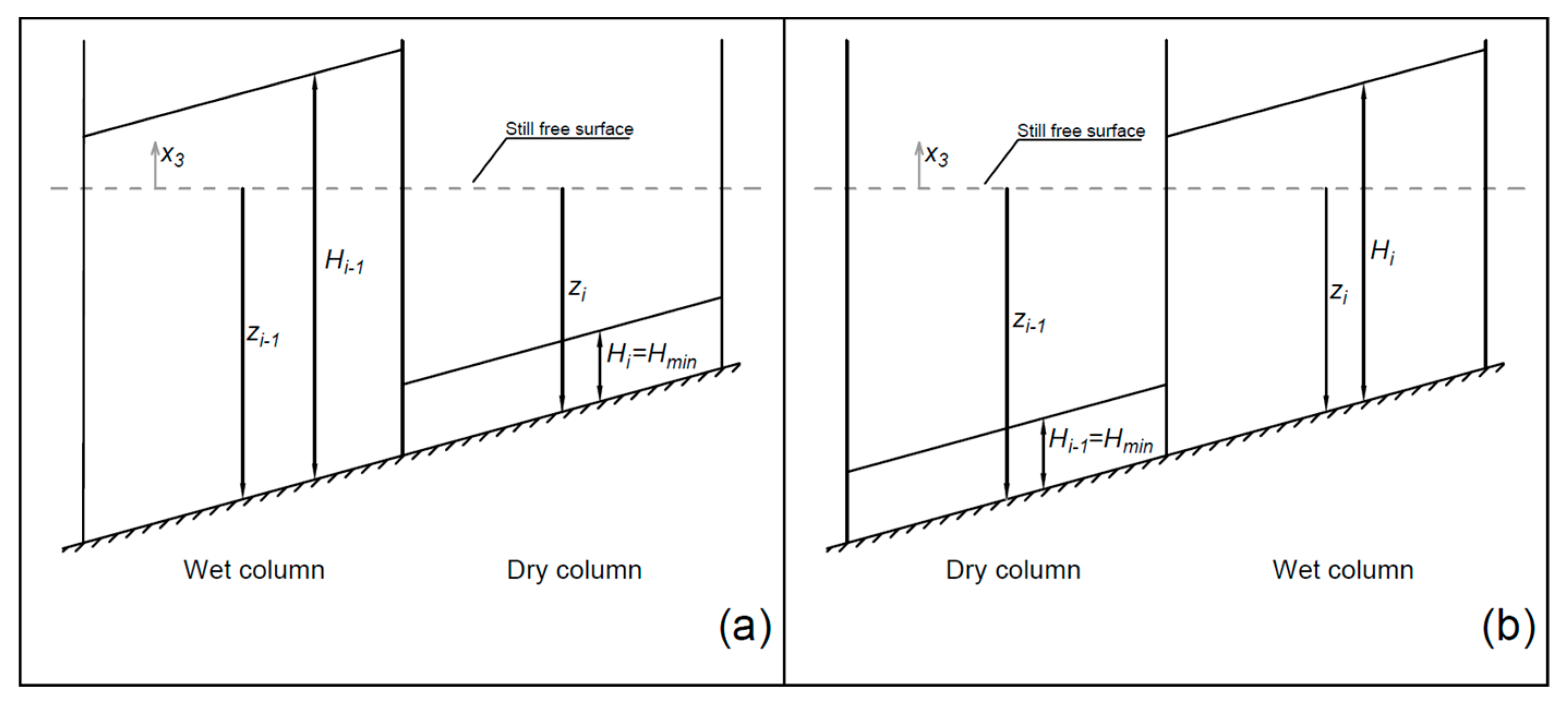
In the adopted numerical model, a novel wet–dry technique is implemented, in order to allow the model to simulate waves propagating over flat or negative slope bottoms. Previous research [15,26] adopted a simple technique proposed by [24] for the treatment of the wet–dry front movement. In order to introduce the aforementioned technique, let us define a column as a set of calculation cells stacked on top of each other, having the same and coordinates. In [15,24,26], a dry column changes its status to wet if its free-surface elevation is less than the free-surface elevation of an adjacent wet column. The aforementioned treatment is proven to be effective in the case in which the wet–dry front propagates over a positive sloping bottom (see Figure 1a), i.e., when at the wet–dry front the bottom elevation of the dry column is greater than the one of the adjacent wet column. Otherwise, if the bottom elevation of the dry column is equal to or less than the one of the adjacent wet column (flat or negative sloping bottom, Figure 1b), the technique proposed by [24] leads to an instantaneous wetting of the subsequent dry columns with bottom elevation equal to or less than the one of the first wet column. This would lead to a thin-film treatment, in which the dry state is treated as a wet state with a thin layer of water; as stated by [33], the thin-film technique fails to correctly evaluate the celerity of the wet–dry front.
In the context of the study of the wave overtopping over barriers, the bottom can have a zero or negative slope. In order to avoid the aforementioned drawback, the following wet–dry procedure has been implemented in the numerical scheme. For the sake of simplicity, the technique is described for the direction. Let be the two indexes which define the center of the calculation cells in the and directions, respectively. Hereinafter, the superscript indicates the time level of the known variables, while the superscript indicates the time level , of the unknown variables. Let us define the column as the set of calculation cells stacked on top of each other, having the same index. The water depth in a wet column is always greater than a minimum water depth, . In a dry column . Let be a dry column and a wet column. The criterion by means of which changes status from dry to wet is described as follows.
Reconstructions defined at the cells that form the wet column lead to point-value variables and , located at the wet–dry cell interfaces. Reconstructions defined at the cells that form the dry column are not carried out and their point-value variables are set to zero. We evaluate as the average of over .
In order to have an estimate of the wet–dry front celerity , the exact solution of the wet–dry Riemann problem over a dry bed is used, adopting piecewise constant initial data, and :
in which represents the position in the direction of the interface between the columns and . From [33], we have:
Is to be noted that the standard solution of the Riemann problem over wet bed, with nonzero water depth in the initial data, cannot be used, since it would lead to a wrong celerity evaluation. See [33] for the details about the wet–dry Riemann problem solution.
Knowing the wet–dry front celerity from Equation (30), the distance between and the wet–dry front is:
The column becomes wet if the wet–dry front reaches the successive column interface, so that
where is the calculation cell dimension in the direction. The above described procedure is repeated in the direction.
It can be noted that, by using the proposed wet–dry technique, the celerity of the wet–dry wave front is used to evaluate the time in which the subsequent dry cell becomes wet. In this way, in case of a flat or negative sloping bottom, a dry column does not instantaneously change status to wet.
3. Experimental Setup
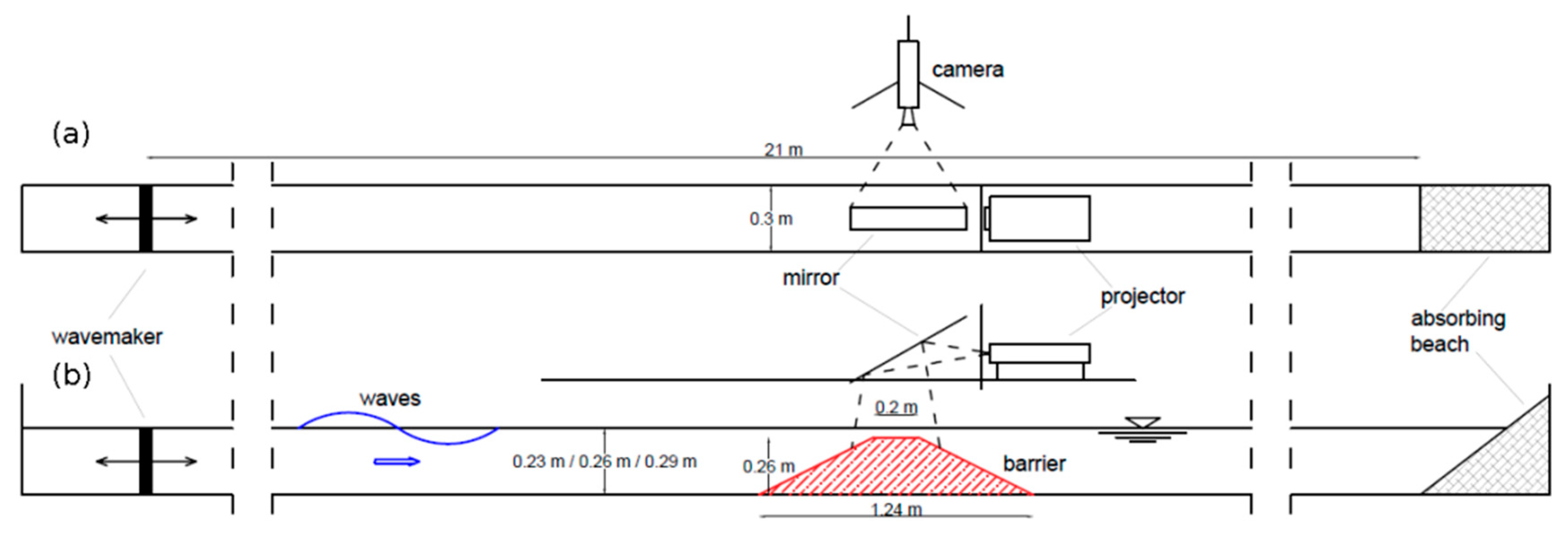
The laboratory tests to validate the numerical model were carried out in a long, wide and high flume, with glass walls, a piston-type wave-maker and an absorbing beach designed to minimize the reflections. The wavemaker is controlled by an in-house developed software, so that monochromatic regular wave trains are produced. The software controls the wave period and amplitude. See Figure 2 for the details of the experimental setup. More details on the wavemaker and flume can be found in [30,34].
The model breakwater employed in the numerical simulations was reproduced by means of a black-painted trapezoidal obstacle of Perspex. Three hydrostatic water depths were employed (, and ). The water was seeded with a fluorescent dye, the investigation area was lighted with a light sheet and images of the experiments were recorded by a digital video camera placed orthogonal to the investigation area; consequently, the recorded images showed a bright area (water) and a dark area (background and breakwater). A set of runs with the same combination of wave periods ( and ), wave heights (, and ) and hydrostatic water levels of the numerical tests was performed.
In order to not modify the flow and to overtake the issues related to traditional probes with very shallow water or breaking waves, an image-analysis technique was developed to identify the free surface. Image-analysis techniques [34,35] have many advantages when compared to traditional probes, as they are nonintrusive (i.e., the flow is not altered by the probes) and quasicontinuous in space (i.e., a measure can be obtained on every pixel on the recorded images). A review can be found in [36].
4. Results and Discussion
4.1. Numerical Simulation Details
All the numerical simulations were run on a 12-CPU workstation using the Message Passing Interface (MPI) procedure. In all the numerical simulations, of the computational time was spent for the solution of the Poisson-like equation in the velocity correction step of the numerical procedure. For this reason, a multigrid V-cycle accelerator was used in the numerical model (see Section 2.2), in order to reduce the simulation time.
4.2. Three-Dimensional Validation Test
In order to validate the three-dimensional nonhydrostatic numerical model presented, we reproduced the experimental test performed by [37] on a fixed submerged barrier with periodically spaced rip channels.
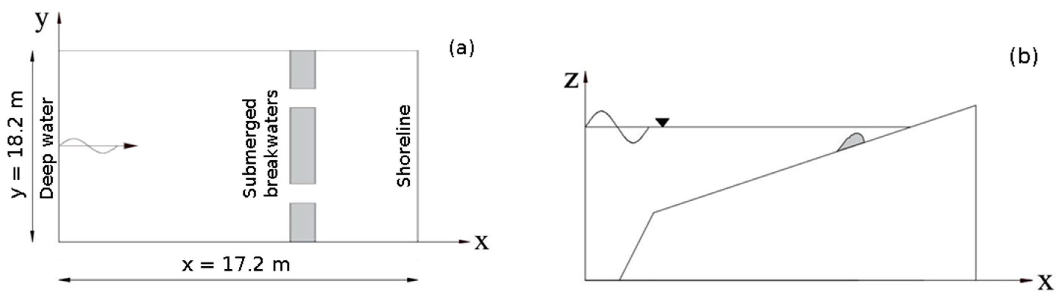
According to [37], the basin is characterized by a length equal to and width equal to . The beach has an initial steep slope (1:5) followed by a milder slope (1:30). There are three submerged breakwaters: the two lateral ones are long, and the central one is long. The distance between the submerged breakwaters is . The seaward edges of the bar sections are located at approximately with the bar crest at and their shoreward edges at . In Figure 3, a plain view and a longitudinal section of the basin for the experimental test performed by [37] are shown.
Regular monochromatic waves are generated at the offshore boundary of the domain. The test parameters are deep water wave height , wave period , average water depth at the bar crest and cross-shore location of the still water line . The computational grid resolution is , and six layers are used in the vertical direction. The time step is . The simulation was carried on for a simulated time of , and ran for four days. After , the hydrodynamic field is supposed to be quasistationary, so the time-averaging of the hydrodynamic quantities is carried out in the interval .
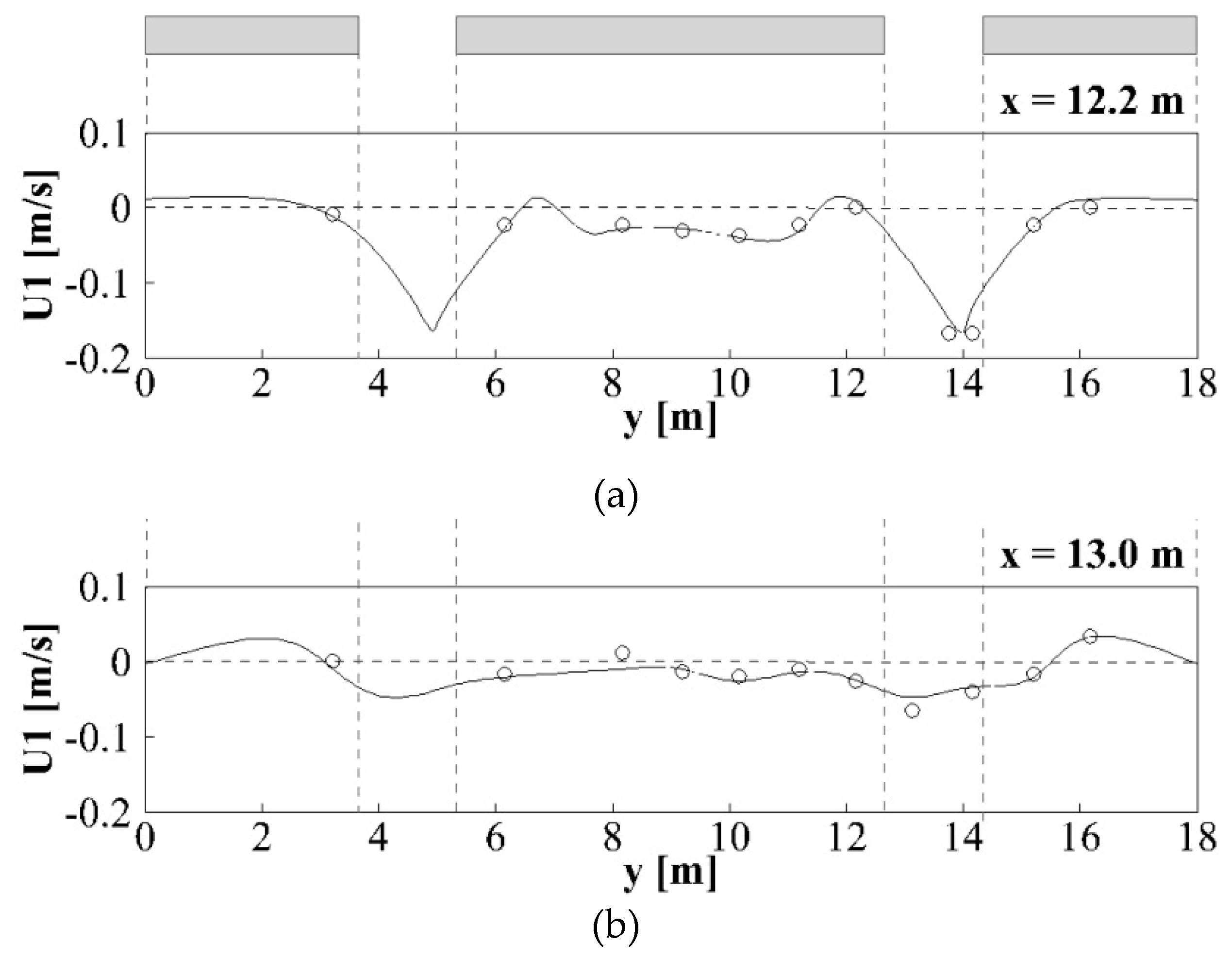
Figure 4 shows a comparison of the cross-shore currents at two different longshore sections: the first at (onshore side of the bar) and the second at (between the bar and the shoreline). From Figure 4, it can be seen that at the onshore side of the bar (), the agreement between the numerical results and the measurements obtained by [37] is good; from Figure 5, it can be seen that in the onshore zone (), the numerical results are in quite good accordance with the experimental ones, even if the numerical model slightly overestimates the offshore currents near the gap between the barriers.
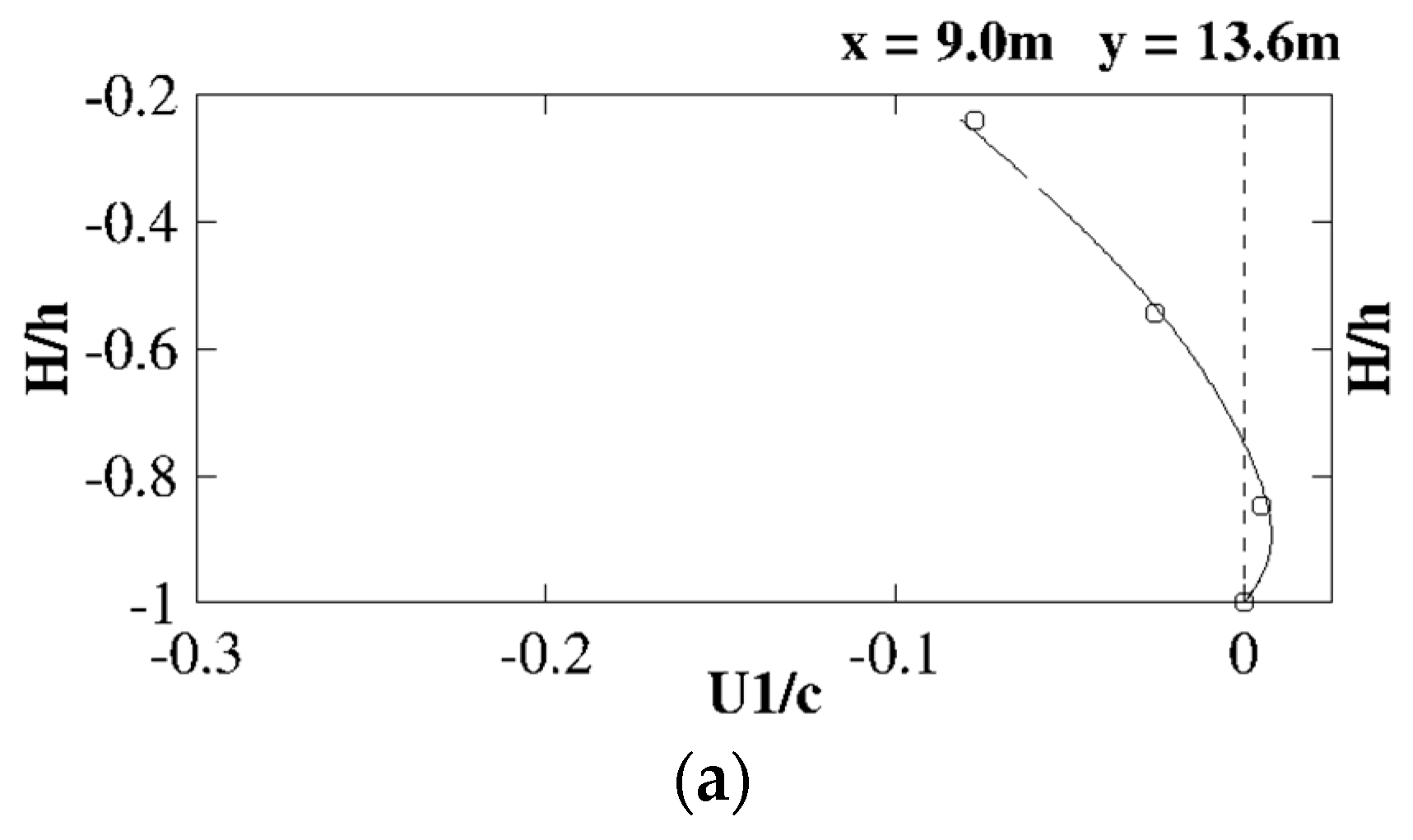
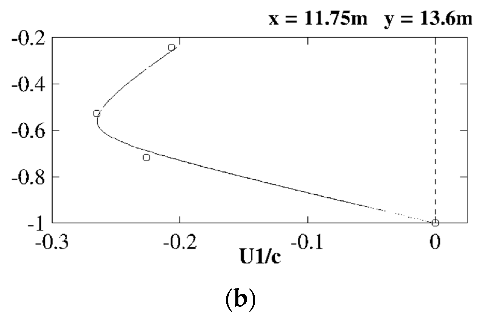
In order to show the ability of the model to reproduce three-dimensional velocity fields, the numerical model is validated against the laboratory measurements of [38], obtained in the same test configuration described above. Figure 5 shows the vertical distribution of time-averaged cross-shore normalized velocity profiles. Normalization is done by dividing the velocity by the celerity . The results are obtained at , ( offshore of the bar) and at , (inside the gap between the bars). Numerical results are compared against the experimental measurements obtained by [38].
From Figure 5, it can be seen that the agreement between the numerical results and experiments is very good. The model is able to reproduce both the offshore current near the free surface in the offshore zone (Figure 5a) and the strong offshore current located at mid-depth in the zone inside the gap between the bars (Figure 5b).
4.3. Wave Overtopping Test
To predict the behavior of waves interacting with the barrier in different configurations, three experimental tests were carried out (see Table 1).
In test T1, mean water depth is lower than barrier height, resulting in an emerged barrier. In test T2, mean water depth is equal to barrier height, resulting in a partially emerged barrier. In test T3, mean water depth is higher than barrier height, resulting in a submerged barrier. For results analysis, phase-averaged free-surface elevation is computed. Numerical tests are carried out with the proposed scheme to reproduce the experiments. For the numerical tests, a fixed time step of , a horizontal spatial step of and six layers in the vertical direction are used. The simulations were carried on for a simulated time of , and ran for approximately 24 h. After , the hydrodynamic field is supposed to be quasistationary, so the phase averaging of the free-surface elevation is carried out in the interval .
4.3.1. Test T1
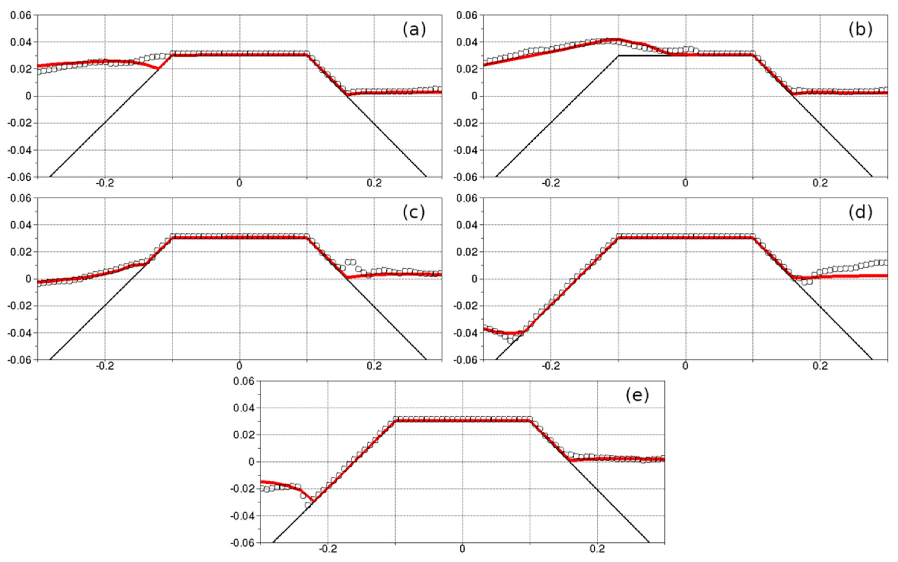
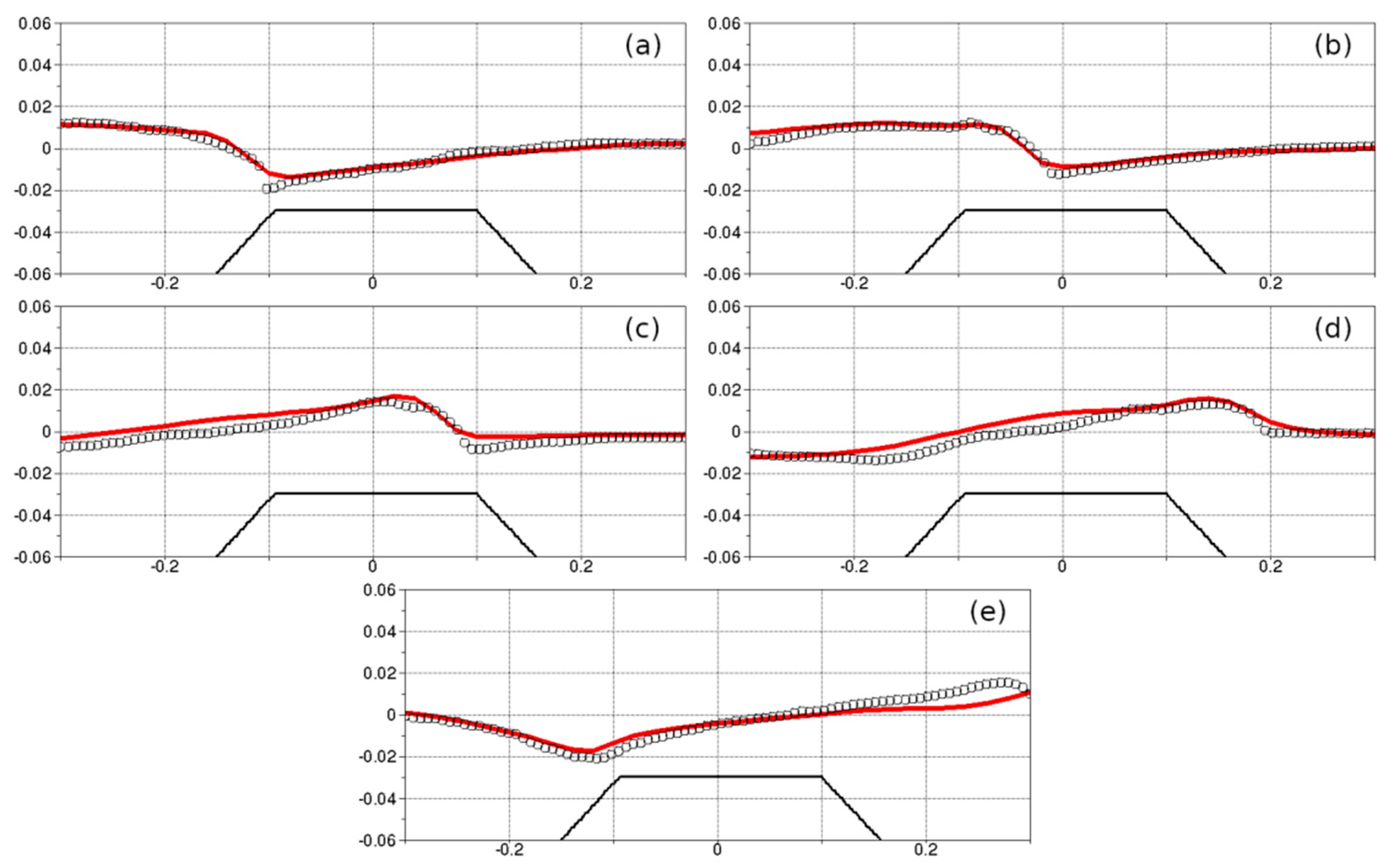
Figure 6 shows the comparison between numerical results and experimental measurements for test T1. It must be noted that the wave is able to pass over the barrier only partially. Figure 6a shows the wave at the end of the run-up phase; the run-up celerity of the wave in the numerical test is slightly lower than the measured one. Figure 6b shows the wave propagation over the crest of the barrier; numerical and experimental results have a good agreement, suggesting that the proposed numerical model is well able to predict front propagation over flat bottoms, thanks to the proposed wet–dry technique. Figure 6c shows that even the simulated wave run-down is in agreement with the measured one. Figure 6d shows the wave trough located at the offshore side of the barrier, while Figure 6e shows the beginning of the run-up phase; Figure 6d,e displays a good accordance between numerical and experimental predictions. Note that in Figure 6c,d, at the onshore side of the barrier, some disturbances of the experimental measurements are present.
4.3.2. Test T2
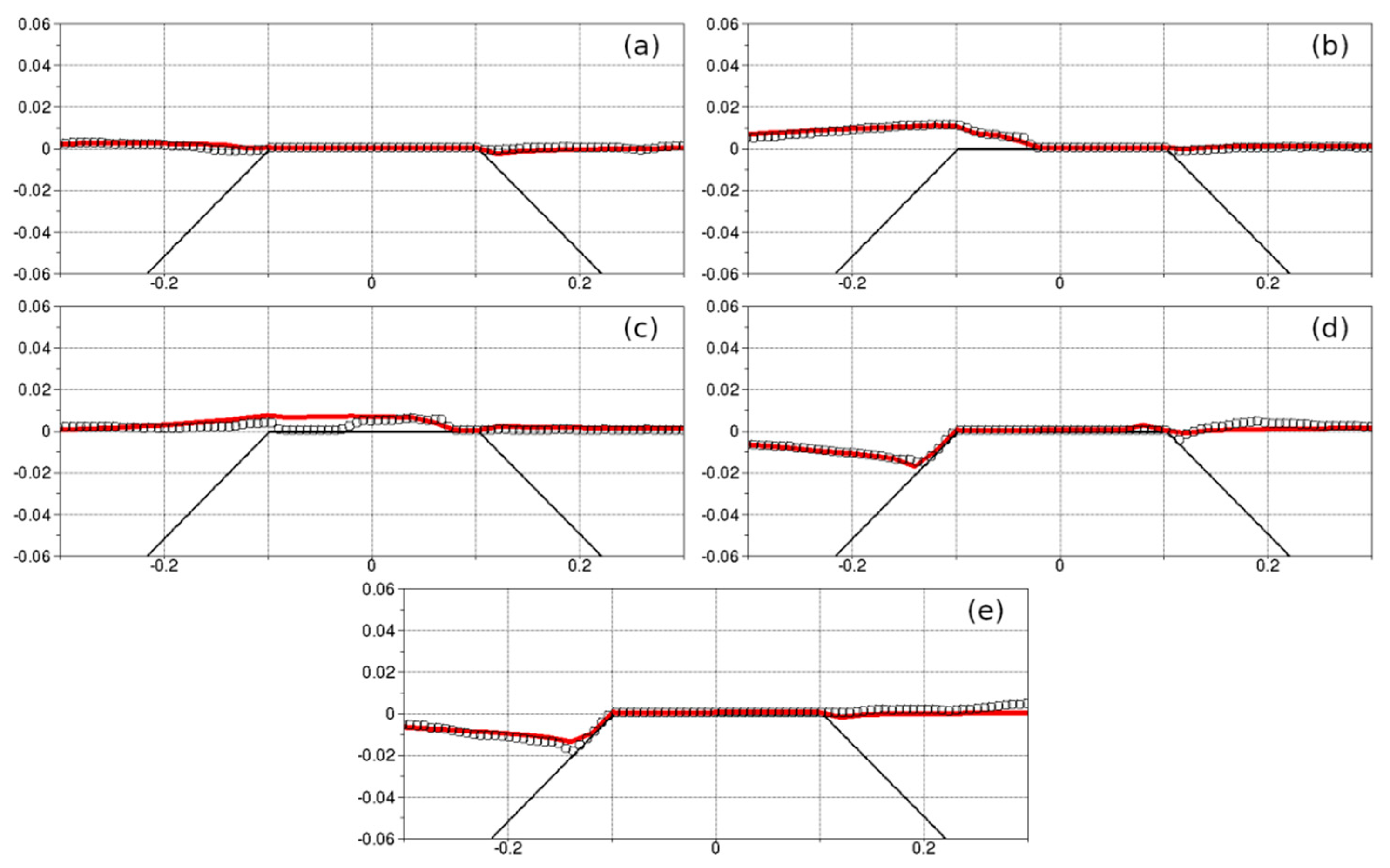
Figure 7 shows the comparison between numerical results and experimental measurements for test T2. In this test, the wave reaches the crest of the barrier with a very shallow water depth. Figure 7a shows the wave run-up over the offshore side of the barrier; as in the test T1, is to be noted that the run-up is well predicted and that numerical and experimental results have a good agreement. Figure 7b,c shows that the proposed wet–dry technique allows the numerical model to reproduce well the wave propagating over the crest of the structure. In Figure 7d, the wave is shown propagating over the inshore side of the barrier crest; numerical and experimental results are in a good agreement, even if is to be noted that experimental results show that the offshore side of the crest is dry. In Figure 7e, the run-down over the offshore side of the barrier is shown, in which numerical and experimental results both well predict the phenomenon.
4.3.3. Test T3
Figure 8 shows the comparison between numerical results and experimental measurements for test T3. In this test, the barrier is completely submerged. Figure 8a,b shows the wave crest propagating over the offshore side of the barrier, with good agreement between numerical and experimental results. In Figure 8c,d, the wave-front propagation over the structure is well reproduced; in the experimental prediction the free surface is slightly higher than in the numerical one. Figure 8e shows the wave crest passing the barrier; is to be noted that in the numerical simulation the wave front has a slightly higher celerity than the predicted experimental celerity.
4.4. Random Wave Overtopping Test
In this subsection, we show the results of several validation tests (described in Table 2), initially proposed by [39], for the proposed numerical model, in the context of wave overtopping by random waves. This is of great practical interest, because, in contrast to regular waves, random waves better represent the complexity of the phenomena found in nature.
The channel is long, with a flat bottom in the first of the channel, and a seawall next to the flat bottom, with a slope angle of . The freeboard is in the first set of three tests and in the second set of three tests. The still water depth is . Random waves are generated by means of the Jonswap spectrum, with a spectral enhancement factor of . According to [39], the input random wave parameters are shown in Table 2. For the numerical simulations, a fixed time step , a horizontal spatial step of and five layers in the vertical direction are used. The simulations ran for approximately 16 h.
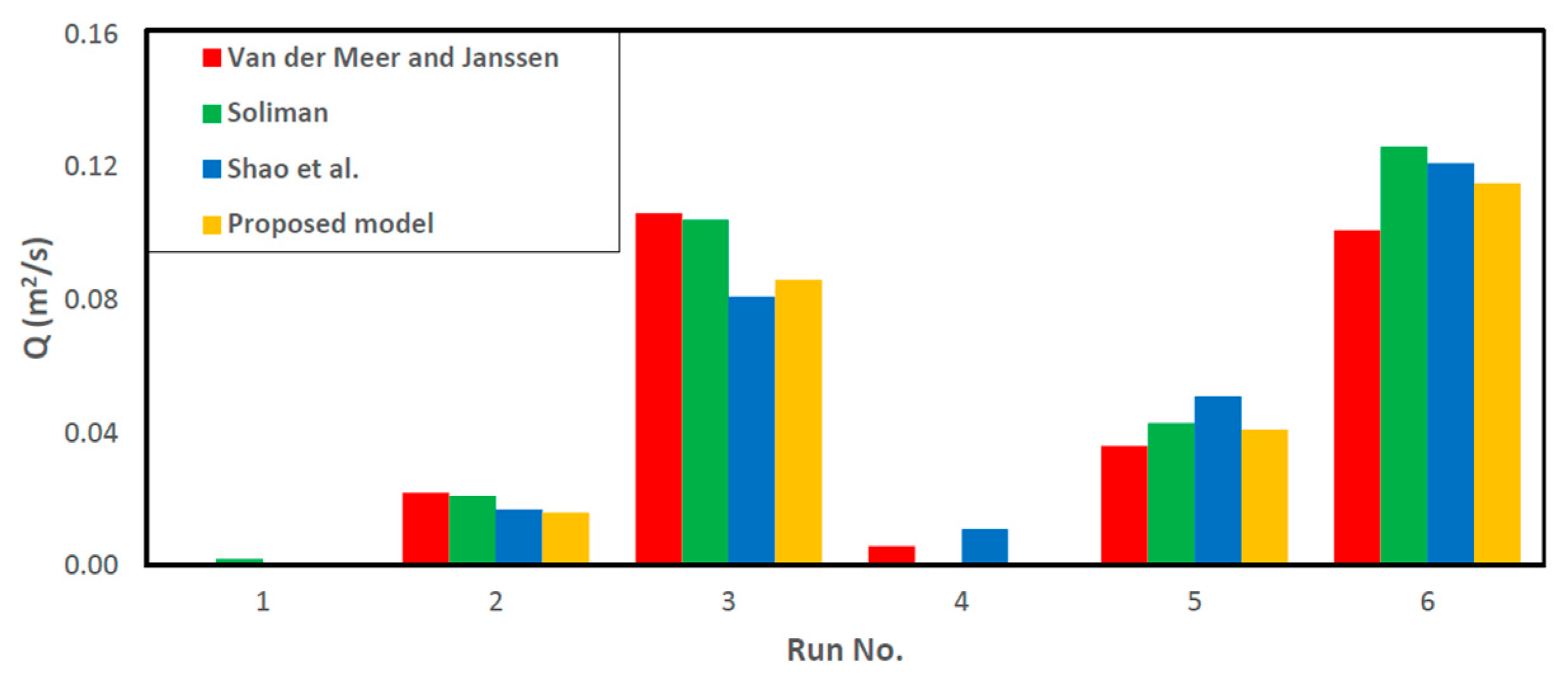
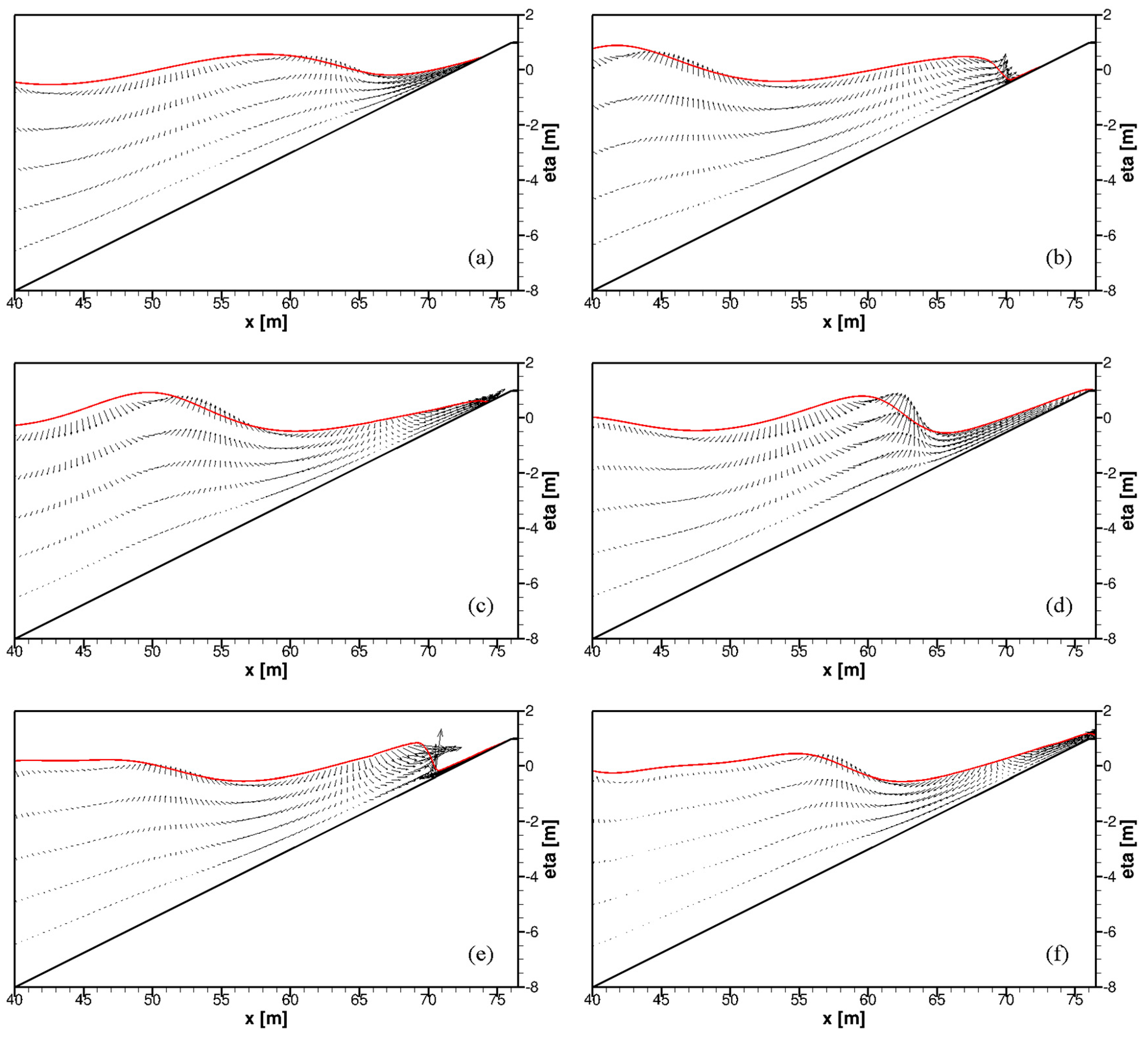
The results obtained by the proposed model, in terms of mean overtopping rate, are compared against the numerical results obtained previously [39,40], and against the results obtained with the wave overtopping formula of [2] (see Figure 9). According to [40], who reproduced the experiment with a Smoothed-Particle Hydrodynamics (SPH) numerical model, the wave overtopping rate becomes stable at approximately . Thus, the mean overtopping rate is calculated in the time interval . The comparison shows that the wave overtopping rate is generally well predicted by the numerical models. The proposed model generally gives a slightly lower prediction than the model proposed by [39]. In the comparison against the prediction formula of [2], the proposed model slightly underestimates the wave overtopping rate in the tests with small wave overtopping, while giving a better prediction in the other tests. In Figure 10, the free-surface elevation and velocity field are shown for test R2 at different instants. The overall shape transformation features of the wave propagating over a slope are shown to be qualitatively well captured.
5. Conclusions
In this work, we presented a numerical and experimental study about the waves overtopping over structures. The numerical model for the simulation of nonhydrostatic free-surface flows proposed by [26] was used and improved, in order to predict the wave overtopping phenomenon. In particular, novel wet–dry technique was implemented in the model, in order to properly calculate the advancement of the wave front over a dry bottom.
The numerical model was validated against several numerical and experimental test cases. Several laboratory tests were carried out, reproducing regular waves overtopping structure, by means of a nonintrusive and continuous-in-space image-analysis technique. Furthermore, in order to evaluate the capacity of the model to simulate phenomena that can be found in nature, the ability to predict the wave and current development over complex structure geometries and the random wave overtopping of structures, were tested. From the numerical tests, it can be assumed that the numerical model is able to reproduce the wave overtopping and wave-front propagation over emerged barriers, for different wave, water-depth and bottom-slope conditions, thanks to the implementation of the proposed wet–dry technique.
Author Contributions
Conceptualization and Methodology, G.C. and M.T.; Validation, Investigation, Writing and Editing, M.G.B., S.F. and M.T.; Supervision, G.Q. and G.C. All authors have read and agreed to the published version of the manuscript.
Funding
This research received no external funding.
Conflicts of Interest
The authors declare no conflict of interest.
References
- Saville, T. Laboratory Data on Wave Run-Up and Overtopping on Shore Structures; Technical Memorandum. No. 64; U.S. Army, Beach Erosion Board, Document Service Center: Dayton, OH, USA, 1955.
- Van der Meer, J.W.; Janssen, J.P.F.M. Wave run-up and wave overtopping at dikes. In Wave Forces on Inclined and Vertical Structures; Demirbilek, Z., Ed.; American Society of Civil Engineers: New York, NY, USA, 1995; Chapter 1; pp. 1–27. [Google Scholar]
- Lorke, S.; Bornschein, A.; Schuttrümpf, H.; Pohl, R. FlowDike-D – Influence of Wind and Current on Wave Run-Up and Wave Overtopping; Technical Report; Rheinisch-Westfälische Technische Hochschule Aachen and Technische Universität Dresden: Aachen, Germany, 2012. [Google Scholar]
- Donatelli, C.; Ganju, N.K.; Karla, T.S.; Fagherazzi, S.; Leonardi, N. Changes in hydrodynamics and wave energy as a result of seagrass decline along the shoreline of a microtidal back-barrier estuary. Adv. Water Res. 2019, 128, 183–192. [Google Scholar] [CrossRef]
- Tonelli, M.; Fagherazzi, S.; Petti, M. Modeling wave impact on salt marsh boundaries. J. Geophys. Res. 2010, 115, 1–17. [Google Scholar] [CrossRef] [Green Version]
- EurOtop. Manual on Wave Overtopping of Sea Defences and Related Structures. An Overtopping Manual Largely Based on European Research, but for Worldwide Application. 2018. Available online: www.overtopping-manual.com (accessed on 10 November 2019).
- Hu, K.; Mingham, C.G.; Causon, D.M. Numerical simulation of wave overtopping of coastal structures using the non-linear shallow water equations. Coast. Eng. 2000, 41, 433–465. [Google Scholar] [CrossRef]
- Cannata, G.; Petrelli, C.; Barsi, L.; Fratello, F.; Gallerano, F. A dam-break flood simulation model in curvilinear coordinates. WSEAS Trans. Fl. Mech. 2018, 13, 60–70. [Google Scholar]
- Kozyrakis, G.V.; Delis, A.I.; Alexandrakis, G.; Kampanis, N. A. Numerical modeling of sediment transport applied to coastal morphodynamics. Appl. Numer. Math. 2016, 104, 30–46. [Google Scholar]
- Kazolea, M.; Delis, A.I. Irregular wave propagation with a 2DH Boussinesq-type model and an unstructured finite volume scheme. Eur. J. Mech. B Fluids 2018, 72, 432–448. [Google Scholar] [CrossRef] [Green Version]
- Tonelli, M.; Petti, M. Shock-capturing Boussinesq model for irregular wave propagation. Coast. Eng. 2012, 61, 8–19. [Google Scholar] [CrossRef]
- Cannata, G.; Barsi, L.; Petrelli, C.; Gallerano, F. Numerical investigation of wave fields and currents in a coastal engineering case study. WSEAS Trans. Fl. Mech. 2018, 13, 87–94. [Google Scholar]
- Tonelli, M.; Petti, M. Numerical simulation of wave overtopping at coastal dikes and low-crested structures by means of a shock-capturing Boussinesq model. Coast. Eng. 2013, 79, 75–88. [Google Scholar] [CrossRef]
- Chen, X. A fully hydrodynamic model for three-dimensional free-surface flows. Int. J. Numer. Meth. Fl. 2003, 42, 929–952. [Google Scholar] [CrossRef]
- Cannata, G.; Petrelli, C.; Barsi, L.; Gallerano, F. Numerical integration of the contravariant integral form of the Navier–Stokes equations in time-dependent curvilinear coordinate systems for three-dimensional free surface flows. Continuum Mech. Therm. 2019, 31, 491–519. [Google Scholar] [CrossRef] [Green Version]
- Lara, J.; Losada, I.J.; del Jesus, M.; Barajas, G.; Guanche, R. IH-3VOF: A three-dimensional Navier-Stokes model for wave and structure interaction. In Proceedings of the 32nd Conference on Coastal Engineering, Shanghai, China, 30 June–5 July 2010. [Google Scholar]
- Casulli, V.; Cheng, R.T. Semi-implicit finite-difference methods for three-dimensional shallow flow. Int. J. Numer. Meth. Fl. 1992, 15, 1045–1068. [Google Scholar] [CrossRef]
- Bradford, S.F. Numerical Simulation of Surf Zone Dynamics. J. Waterw. Port. Coast. Ocean Eng. 2000, 126, 1–13. [Google Scholar] [CrossRef]
- Van der Meer, J.W.; Petit, H.A.H.; van den Bosch, P.; Klopman, G.; Broekens, R.D. Numerical Simulation of Wave Motion on and in Coastal Structures. In Proceedings of the 23rd International Conference on Coastal Engineering, Venice, Italy, 4–9 October 1992. [Google Scholar]
- Berberović, E.; van Hinsberg, N.P.; Jakirlić, S.; Roisman, I.V.; Tropea, C. Drop impact onto a liquid layer of finite thickness: Dynamics of the cavity evolution. Phys. Rew. E 2009, 79, 1–15. [Google Scholar] [CrossRef]
- Higuera, P.; Lara, J.L.; Losada, I.J. Simulating coastal engineering processes with OpenFOAM®. Coast. Eng 2013, 71, 119–134. [Google Scholar] [CrossRef]
- Lin, P.; Li, C.W. A σ-coordinate three-dimensional numerical model for surface wave propagation. Int. J. Numer. Meth. Fl. 2002, 38, 1045–1068. [Google Scholar] [CrossRef]
- Lin, P. A multiple-layer σ-coordinate model for simulation of wave–structure interaction. Comput. Fl. 2006, 35, 147–167. [Google Scholar] [CrossRef]
- Ma, G.; Shi, F.; Kirby, J.T. Shock-capturing non-hydrostatic model for fully dispersive surface wave processes. Ocean Model. 2012, 43–44, 22–35. [Google Scholar] [CrossRef]
- Cannata, G.; Petrelli, C.; Barsi, L.; Camilli, F.; Gallerano, F. 3D free surface flow simulations based on the integral form of the equations of motion. WSEAS Trans. Fl. Mech. 2017, 12, 166–175. [Google Scholar]
- Cannata, G.; Gallerano, F.; Palleschi, F.; Petrelli, C.; Barsi, L. Three-dimensional numerical simulation of the velocity fields induced by submerged breakwaters. Int. J. Mech. 2019, 13, 1–14. [Google Scholar]
- Armenio, E.; Ben Meftah, M.; Bruno, M.F.; De Padova, D.; De Pascalis, F.; De Serio, F.; Di Bernardino, A.; Mossa, M.; Leuzzi, G.; Monti, P. Semi enclosed basin monitoring and analysis of meteo, wave, tide and current data: Sea monitoring. In Proceedings of the EESMS 2016—2016 IEEE Workshop on Environmental, Energy, and Structural Monitoring Systems, Bari, Italy, 13–14 June 2016; p. 7504835. [Google Scholar]
- Bruno, D.; De Serio, F.; Mossa, M. The FUNWAVE model application and its validation using laboratory data. Coast. Eng. 2009, 56, 773–787. [Google Scholar] [CrossRef]
- De Padova, D.; Brocchini, M.; Buriani, F.; Corvaro, S.; De Serio, F.; Mossa, M.; Sibilla, S. Experimental and numerical investigation of pre-breaking and breaking vorticity within a plunging breaker. Water 2018, 10, 387. [Google Scholar] [CrossRef] [Green Version]
- Ferrari, S.; Badas, M.G.; Querzoli, G. A non-intrusive and continuous-in-space technique to investigate the wave transformation and breaking over a breakwater. In Proceedings of the EPJ Web of Conferences, EFM15 – Experimental Fluid Mechanics 2015, Prague, Czech Republic, 17–20 November 2015; p. 02022. [Google Scholar]
- Spiteri, R.J.; Ruuth, S.J. A new class of optimal high-order strong-stability preserving time discretization methods. SIAM J. Numer. Anal. 2002, 40, 469–491. [Google Scholar] [CrossRef]
- Trottenberg, U.; Oosterlee, C.W.; Schuller, A. Multigrid; Academic Press: London, UK, 2000. [Google Scholar]
- Toro, E. Shock-Capturing Methods for Free-Surface Shallow Flows; John Wiley and Sons: Manchester, UK, 2001. [Google Scholar]
- Ferrari, S.; Querzoli, G. Laboratory experiments on the interaction between inclined negatively buoyant jets and regular waves. In Proceedings of the EPJ Web of Conferences, EFM14 – Experimental Fluid Mechanics 2014, Český Krumlov, Czech Republic, 18–21 November 2014; Volume 92, p. 02018. [Google Scholar] [CrossRef] [Green Version]
- Besalduch, L.A.; Badas, M.G.; Ferrari, S.; Querzoli, G. On the near field behavior of inclined negatively buoyant jets. In Proceedings of the EPJ Web of Conferences, EFM13 – Experimental Fluid Mechanics 2013, Kutná Hora, Czech Republic, 19–22 November 2013; p. 02007. [Google Scholar]
- Ferrari, S. Image analysis techniques for the study of turbulent flows. In Proceedings of the EPJ Web of Conferences, EFM16 – Experimental Fluid Mechanics 2016, Marienbad, Czech Republic, 15–18 November 2016; Volume 143, p. 01001. [Google Scholar] [CrossRef] [Green Version]
- Haller, M.C.; Dalrymple, R.A.; Svendsen, I.A. Experimental study of nearshore dynamics on a barred beach with rip channels. J. Geophys. Res. 2002, 107, 1–21. [Google Scholar] [CrossRef] [Green Version]
- Haas, K.A.; Svendsen, I.A. Laboratory measurements of the vertical structure of a rip current. J. Geophys. Res. 2002, 107, 1–19. [Google Scholar] [CrossRef]
- Soliman, A. Numerical Study of Irregular Wave Overtopping and Overflow. Ph.D. Thesis, The University of Nottingham, Nottingham, UK, 2003. [Google Scholar]
- Shao, S.; Ji, C.; Graham, D.I.; Reeve, D.E.; James, P.W.; Chadwick, A.J. Simulation of wave overtopping by an incompressible SPH model. Coast. Eng. 2006, 53, 723–735. [Google Scholar] [CrossRef]
Figure 1.
Positive and negative sloping bottoms. (a) Positive sloping bottom and (b) negative sloping bottom.
Figure 1.
Positive and negative sloping bottoms. (a) Positive sloping bottom and (b) negative sloping bottom.

Figure 2.
Experimental setup. (a) Plan view and (b) longitudinal section.

Figure 3.
Experimental test carried out by [37]. (a) Plan view and (b) longitudinal section.
Figure 3.
Experimental test carried out by [37]. (a) Plan view and (b) longitudinal section.

Figure 4.
Cross-shore currents at x = 12.20 m (a) and at x = 13.00 m (b). Circles: experimental results by [37]. Solid line: proposed numerical model.
Figure 4.
Cross-shore currents at x = 12.20 m (a) and at x = 13.00 m (b). Circles: experimental results by [37]. Solid line: proposed numerical model.

Figure 5.
Vertical distribution of cross-shore currents at x = 9.00 m, y = 13.60 m (a) and at x = 11.75 m, y = 13.60 m (b). Circles: experimental results by [38]. Solid line: proposed numerical model.
Figure 5.
Vertical distribution of cross-shore currents at x = 9.00 m, y = 13.60 m (a) and at x = 11.75 m, y = 13.60 m (b). Circles: experimental results by [38]. Solid line: proposed numerical model.


Figure 6.
Test T1. Phase-averaged free-surface elevation. (a) t/T = 0.0; (b) t/T = 0.2; (c) t/T = 0.4; (d) t/T = 0.6; (e) t/T = 0.8. Circles: experimental results. Red line: numerical results.
Figure 6.
Test T1. Phase-averaged free-surface elevation. (a) t/T = 0.0; (b) t/T = 0.2; (c) t/T = 0.4; (d) t/T = 0.6; (e) t/T = 0.8. Circles: experimental results. Red line: numerical results.

Figure 7.
Test T2. Phase-averaged free-surface elevation. (a) t/T = 0.0; (b) t/T = 0.2; (c) t/T = 0.4; (d) t/T = 0.6; (e) t/T = 0.8. Circles: experimental results. Red line: numerical results.
Figure 7.
Test T2. Phase-averaged free-surface elevation. (a) t/T = 0.0; (b) t/T = 0.2; (c) t/T = 0.4; (d) t/T = 0.6; (e) t/T = 0.8. Circles: experimental results. Red line: numerical results.

Figure 8.
Test T3. Phase-averaged free-surface elevation. (a) t/T = 0.0; (b) t/T = 0.2; (c) t/T = 0.4; (d) t/T = 0.6; (e) t/T = 0.8. Circles: experimental results. Red line: numerical results.
Figure 8.
Test T3. Phase-averaged free-surface elevation. (a) t/T = 0.0; (b) t/T = 0.2; (c) t/T = 0.4; (d) t/T = 0.6; (e) t/T = 0.8. Circles: experimental results. Red line: numerical results.

Figure 9.
Wave overtopping rate. Red: calculated by the Van der Meer and Janssen laboratory formula [2]; green: computed by Soliman [39]; blue: computed by Shao et al. [40]; yellow: computed with the proposed model.

Figure 10.
Free-surface elevation and velocity field for test R2. (a) ; (b) ; (c) ; (d) ; (e) ; (f) .
Figure 10.
Free-surface elevation and velocity field for test R2. (a) ; (b) ; (c) ; (d) ; (e) ; (f) .


Table 1.
Regular wave overtopping test configurations.
| Test | Mean Water Depth (m) | Wave Height (cm) | Wave Period (s) |
|---|---|---|---|
| T1 | 0.23 | 3.5 | 1.55 |
| T2 | 0.26 | 1 | 1.55 |
| T3 | 0.29 | 2.5 | 0.95 |
Table 2.
Random waves overtopping test configurations.
| Test | Freeboard (m) | Significant Wave Height (m) | Mean Wave Period (s) | Peak Wave Period (s) |
|---|---|---|---|---|
| R1 | 1.0 | 0.78 | 3.53 | 3.07 |
| R2 | 1.0 | 1.22 | 4.38 | 3.81 |
| R3 | 1.0 | 1.70 | 5.19 | 4.51 |
| R4 | 1.5 | 1.26 | 4.38 | 3.81 |
| R5 | 1.5 | 1.75 | 5.16 | 4.49 |
| R6 | 1.5 | 2.35 | 6.03 | 5.24 |
© 2020 by the authors. Licensee MDPI, Basel, Switzerland. This article is an open access article distributed under the terms and conditions of the Creative Commons Attribution (CC BY) license (http://creativecommons.org/licenses/by/4.0/).
Share and Cite
MDPI and ACS Style
Cannata, G.; Tamburrino, M.; Ferrari, S.; Badas, M.G.; Querzoli, G. Numerical and Experimental Investigation of Wave Overtopping of Barriers. Water 2020, 12, 451. https://doi.org/10.3390/w12020451
AMA Style
Cannata G, Tamburrino M, Ferrari S, Badas MG, Querzoli G. Numerical and Experimental Investigation of Wave Overtopping of Barriers. Water. 2020; 12(2):451. https://doi.org/10.3390/w12020451
Chicago/Turabian StyleCannata, Giovanni, Marco Tamburrino, Simone Ferrari, Maria Grazia Badas, and Giorgio Querzoli. 2020. "Numerical and Experimental Investigation of Wave Overtopping of Barriers" Water 12, no. 2: 451. https://doi.org/10.3390/w12020451
Note that from the first issue of 2016, this journal uses article numbers instead of page numbers. See further details here.