The Impact of Capillary Trapping of Air on Satiated Hydraulic Conductivity of Sands Interpreted by X-ray Microtomography


1
Faculty of Civil Engineering, Czech Technical University in Prague, 166 29 Prague, Czech Republic
2
Laboratório de Métodos de Modelagem e Geofísica Computacional, Universidade Federal do Rio de Janeiro, Rio de Janeiro 21941-596, Brazil
3
Department of Soil and Environment, Swedish University of Agricultural Sciences, 750 07 Uppsala, Sweden
*
Author to whom correspondence should be addressed.
Water 2020, 12(2), 445; https://doi.org/10.3390/w12020445
Submission received: 17 December 2019
/
Revised: 29 January 2020
/
Accepted: 4 February 2020
/
Published: 7 February 2020
(This article belongs to the Special Issue Water Flow, Solute and Heat Transfer in Groundwater)
Abstract
:The relationship between entrapped air content and the corresponding hydraulic conductivity was investigated experimentally for two coarse sands. Two packed samples of 5 cm height were prepared for each sand. Air entrapment was created by repeated infiltration and drainage cycles. The value of K was determined using repetitive falling-head infiltration experiments, which were evaluated using Darcy’s law. The entrapped air content was determined gravimetrically after each infiltration run. The amount and distribution of air bubbles were quantified by micro-computed X-ray tomography (CT) for selected runs. The obtained relationship between entrapped air content and satiated hydraulic conductivity agreed well with Faybishenko’s (1995) formula. CT imaging revealed that entrapped air contents and bubbles sizes were increasing with the height of the sample. It was found that the size of the air bubbles and clusters increased with each experimental cycle. The relationship between initial and residual gas saturation was successfully fitted with a linear model. The combination of X-ray computed tomography and infiltration experiments has a large potential to explore the effects of entrapped air on water flow.
1. Introduction
Interaction between water and gas needs to be considered for water fluxes in near-saturated and saturated soil because the entrapped air may block pores and thereby affect the hydraulic conductivity [1,2,3]. Entrapped air is defined as a discontinuous non-wetting phase that is not connected to the atmosphere [1]. Entrapped air may appear in the form of single pore bubbles, clusters or ganglia [4]. With growing size, such ganglia become more mobile [5] and may escape from the soil to the atmosphere. The pressure in the discontinuous air phase usually differs from the atmospheric pressure [6] and can be measured from the curvature of the water–air interface.
We distinguish between three states of saturation. If the pressure in the soil water is lower than the air entry value, the soil is denoted as unsaturated soil. In this state, it contains a continuous air phase with connection to and in equilibrium with the atmosphere. Quasi-saturated [1] or satiated [7] soil contains air in the form of entrapped air bubbles or air ganglia with water pressures higher than the air entry value [6]. Fully saturated soil, which is rarely found under natural conditions, does not contain any air bubbles or ganglia. The amount of entrapped air in porous media is commonly expressed as a residual gas saturation, Sg,r (–), or an entrapped volumetric air content [1], ω (–). The residual gas saturation is the ratio of entrapped air volume to the volume of pores. The entrapped air content is the ratio of entrapped air volume to the bulk volume of soil.
Chatzis et al. [8] define two main mechanisms of non-wetting phase trapping in porous media, termed (i) distinguished-bypassing and (ii) snap-off trapping. Distinguished-bypassing results from the fact that smaller throats are filled with water before larger ones are, due to capillary forces. If a larger pore containing gas is surrounded by water-filled throats, the gas is entrapped. According to Almajid and Kovscek [9], snap‑off trapping is a hydraulic process where the wetting phase forms blockages in the pore throat that snap-off gas bubbles as they move through the pore throat. The snap-off mechanism is present predominantly in pore networks with a large aspect ratio, i.e., ratios between pore–body and pore–throat sizes, and seems to be the dominant mechanism in the formation of a discontinuous gas phase within such porous media [10].
The amount of the entrapped non-wetting phase in porous media depends predominantly on the pore structure [8], but also on the history of wetting and drying [11,12] as well as the contact angle [5,13]. Higher values of the contact angle lead to a suppression of the snap-off mechanism, resulting in a smaller amount of entrapped air. Furthermore, it has been shown that the Sg,r value is positively correlated with the initial gas saturation, Sg,init, when porous media is imbibed [14]. Distribution of the air bubbles may be affected by temperature [15].
Generally, it has been assumed that the Sg,r value is constant [16]. However, Hilfer [17] showed that the Sg,r value is a function of the time and position. He builds a formulation of two-phase immiscible displacement based on the general balance laws. Used assumptions were that the porous medium is macroscopically homogeneous, the fluid is incompressible, the flow has low Reynolds number and body forces are given by gravity and capillary forces.
The presence of entrapped air in soil introduces ambiguity for the definition and measurements of hydraulic conductivity close to saturation. Given the states of saturation, the hydraulic conductivity may be specified as saturated, KS (cm∙s−1), satiated, K(ω) (cm∙s−1), or unsaturated, K(θ) (cm∙s−1). A widely used model that calculates the unsaturated hydraulic conductivity function from the soil water content and the saturated hydraulic conductivity was introduced by Mualem [18]. It represents an estimate of the relative hydraulic conductivity function Kr(θ) = K(θ)/Ks (–) based on the capillary model theory [19]. The water retention curves are modeled by the approaches of either Brooks and Corey [20] or van Genuchten [21]. Another model for the satiated hydraulic conductivity was presented by Faybishenko [1].
Laboratory experiments have shown that hydraulic conductivity depends significantly on the entrapped air content ω [22,23,24]. In a laboratory study on small soil samples, Sakaguchi et al. [25] showed that the measured satiated hydraulic conductivity, K(ω), was smaller than the unsaturated hydraulic conductivity, K(θ), although the same amount of air was entrapped. The authors explained this by entrapped air clogging of the largest pores. The effect of entrapped air on infiltration in the field was also confirmed by Alagna et al. [26].
For a long term infiltration experiment carried out on large soil monoliths, Faybishenko [1] observed three stages in which the hydraulic conductivity changed characteristically. During the first stage, the value of the hydraulic conductivity decreased. Faybishenko presumed that at the beginning, the air was entrapped in small pores. But due to the capillary forces, water started to infiltrate into the smaller pores of the matrix. The air was thus continuously displaced into larger pores, forming entrapped air bubbles that then blocked preferential flow pathways. In the second stage, the hydraulic conductivity value started to increase again due to the dissolution of gas bubbles. In the third stage of the experiment, the hydraulic conductivity decreased again, this time due to the buildup of biofilms created by microbial activity.
A fundamental improvement in the description of processes connected with the flow of liquids in porous media was achieved with the possibility to use nondestructive visualization techniques. Noninvasive imaging can be used to obtain information about the distribution of the wetting and non-wetting phases [27].
Snehota et al. [3] illustrated and quantified air redistributions during infiltration experiments in a repacked sand sample using neutron imaging. The sand sample contained blocks of fine sand surrounded by coarse sand. Snehota et al. [3] found that entrapped air was transferred from the fine into the coarse sand while the flow rate decreased from 0.400 cm∙min−1 to 0.296 cm∙min−1. Similar results were obtained in an experiment with a similarly designed sand sample [2] on which repeated infiltration runs were performed. Also here, the redistribution of entrapped air from the finer to the coarser sand caused the infiltration rate to slow down. The flow rate decreased from 3.7 cm∙h−1 to 1.0 cm∙h−1 during the first infiltration run and during the second infiltration run from 3.6 to 1.6 cm∙h−1. Thereafter, an infiltration run with degassed water was performed during which the flow rate increased to a maximum value of 10.5 cm∙h−1.
A frequently used imaging technique in porous media research is synchrotron‑based X-ray tomography. Taking advantage of its high image resolution, it was often applied to obtain pore geometry properties [28,29,30], aggregate microstructures [31,32,33] and multi-phase flow observations [34,35]. Industrial X-ray scanners are also suited to collect detailed information on soil structure development [36,37] or gas bubbles distribution [38,39,40,41,42]. A disadvantage of industrial X-ray scanners is that they operate with polychromatic X-rays, which may cause beam hardening artifacts [43,44].
Hydraulic conductivity is a crucial parameter in all components of water cycle modeling, rainfall excess determination, water and solute transport in vadose zone as well as in recharge of groundwater [26,45,46,47]. The impact of entrapped air on measured values of satiated hydraulic conductivity means that instead of a well-defined constant parameter, its value may vary in dependence on many factors, some of them described in this paper.
This study aimed to unravel the relationship between the entrapped air content and the dependence of the air trapping on the initial air saturation in two coarse sands. Recent experimental studies [3,48] on air entrapment involved the same sands as components of more complex, heterogeneous samples. To enable numerical modeling of these experiments in future, the K(ω) relationship of coarse sands is needed. An additional goal of the current study was to investigate variations of the entrapped air bubbles in space and time during repeated infiltration drainage cycles. Experiments were conducted on packed samples of coarse sand representing homogeneous media with narrow pore size distribution to rule out the effects of heterogeneity. The aim was to use X‑ray computed micro-tomography to characterize the sizes, shapes and abundance of entrapped air bubbles.
2. Materials and Methods
2.1. Material Characterization
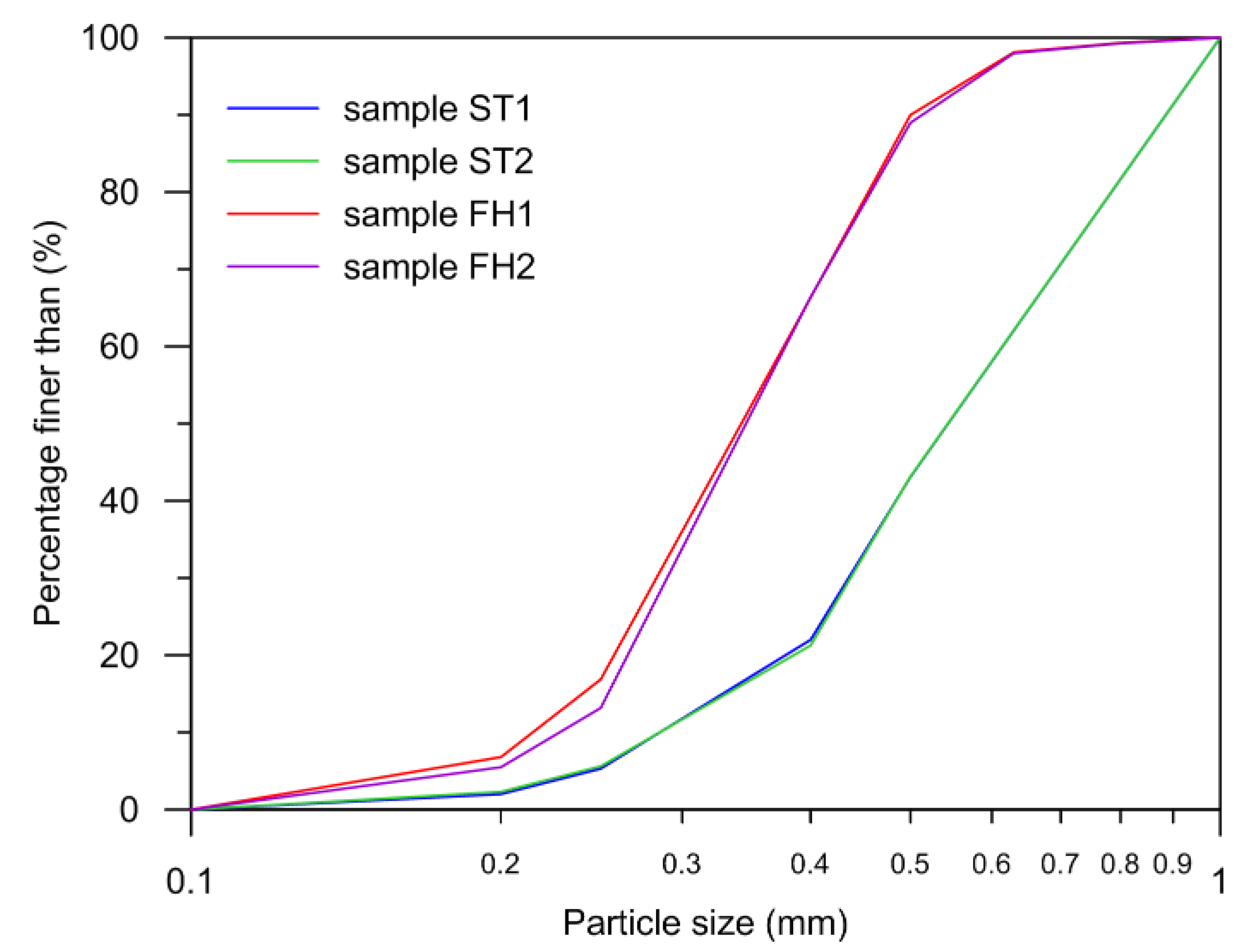
We prepared four packed samples, each two with different sands that we denote with abbreviations ST and FH, respectively. The ST sand is a commercially available technical quartz sand—with a SiO2 content 99.40% and Fe2O3 content 0.04% (technical designation ST 03/08, Sklopisek Strelec, Czech Republic). The FH sand is a commercially produced quartz sand from with a SiO2 content of larger than 99% (technical designation FH31, Quarzwerke Frechen, Germany). We evaluated the grain-size distribution of the two different sands by dry sieving. Here we employed mesh-sizes of 0.20, 0.25, 0.40, 0.50, 0.63, 0.80, and 1.00 mm. The particle densities were measured using a pycnometer and turned out to be identical 2.62 g∙cm−3 for all samples. The dry bulk densities of the samples were calculated from the mass and volume of dry sand samples. The samples’ porosities were determined from the particle densities and the dry bulk densities. The grain size distributions of all samples are shown in Figure 1. Table 1 contains the respective values of dry bulk density, porosity as well as packing height and sample volume. The FH sand is finer and has a lower porosity than the ST sand. The value of the uniformity coefficient (D60/D10, where Dx represents the size for which x% particles are smaller) for ST sand was 2.2 and for FH sand the value was 1.7. Both sands are considered to be poorly graded, but the FH sand is more uniform. The effective size (D10) of the ST sand is 0.29 mm and of the FH sand is 0.22 mm.
2.2. Experimental Setup
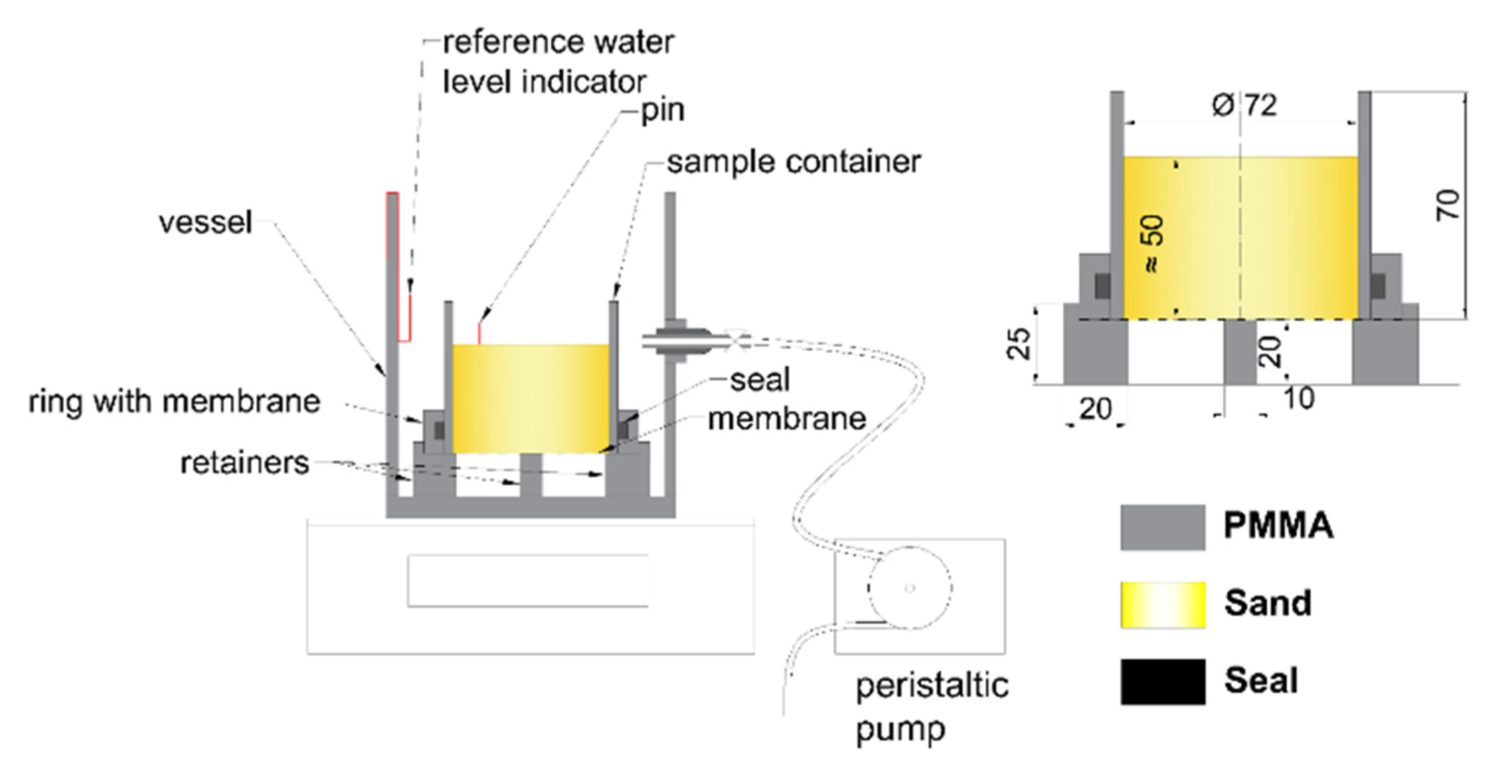
The saturated and satiated hydraulic conductivity of sand were measured with repetitive falling-head infiltration experiments. The respective setup is presented in Figure 2. The sample container consisted of an acrylic glass (PMMA) cylinder (7.2 cm inner diameter, 7.0 cm height) and a PMMA ring with a filter-mesh (size 99 µm) attached to its bottom. An o-ring made of nitrile rubber was used as a hydraulic seal, ensuring no water could escape between the ring and cylinder. The sample container was filled with the sand up to the height of approximately 5.0 cm. The container was placed into a larger, outer PMMA vessel (inner diameter 12.3 cm), where it was mounted onto five PMMA retainers. An overflow was inserted into the wall of the outer vessel (WADI-PZ, M12×1.5, 3.0–6.5 mm, Hugro Plastic Cable Gland, Waldkirch, Germany) through which a constant water level could be kept. To achieve a sufficiently large flow rate through the overflow, we attached a tube connected to a peristaltic pump (see Figure 2). The vessel was placed on a balance with 0.1 g precision to monitor the amount of water and gas in the outer vessel and the sample.
2.3. Sample Preparation
Two samples (ST1 and ST2) were packed with ST sand, while another two samples (FH1 and FH2) were prepared with FH sand. The samples were packed to a height of approximately 5.0 cm (the exact heights are given in Table 1) into cylindrical containers with an inner diameter of 7.2 cm. The sand packing was performed in degassed, deionized water, to minimize the introduction of entrapped air bubbles. The sand was added in 20 steps. After each addition step, the sand in the column was compacted by a small manual compactor, consisting of a rubber stopper and rod. The saturation by vacuum was used to ensure full saturation of the sand in the column [49]. The vessel with a submerged sample container was inserted into a vacuum chamber. The vacuum chamber was then evacuated for approximately 20 min at −95 kPa (relative to the atmospheric pressure). To minimize changes in pore geometry due to the resulting air bubble ebullition, a perforated plate loaded with 1.24 kg weight was placed on the sample’s surface during this process.
2.4. Determination of Saturated Hydraulic Conductivity
To determine the value of saturated hydraulic conductivity, the first infiltration experiment with the repetitive falling-head was performed on the fully saturated sample, directly after it had been removed from the vacuum chamber. We assumed that the entrapped air content ω was zero at this point. The water used in infiltration experiments was kept in an open bottle one day before the experiment in order to equilibrate the temperature and dissolved air content to the laboratory conditions.
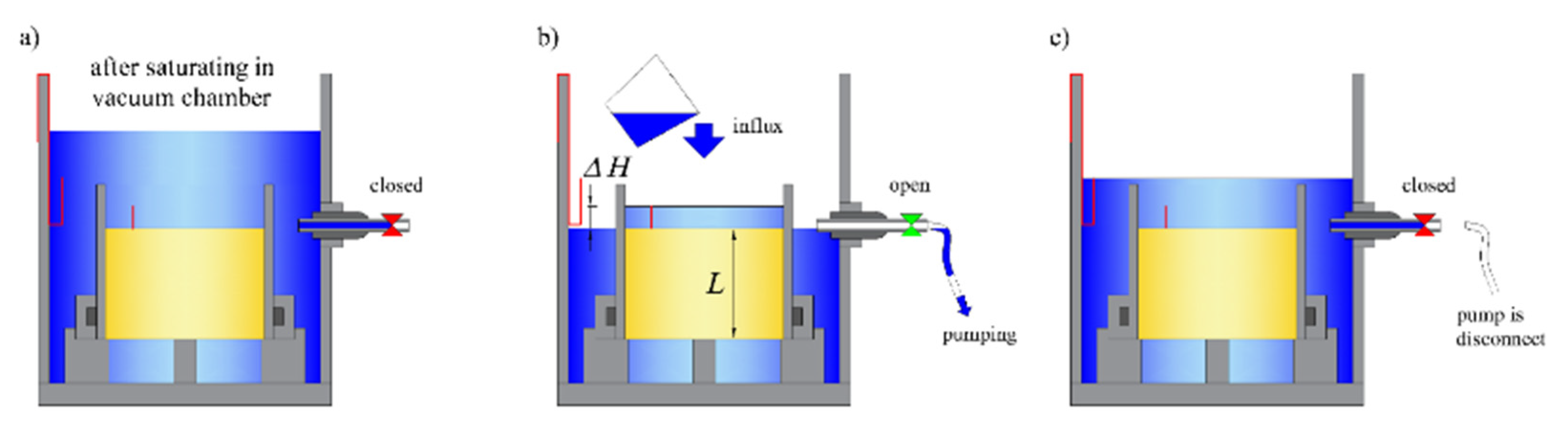
The workflow of the infiltration experiments is shown in Figure 3. At the first stage (Figure 3a), the sample container was submerged in degassed water. Then a simple repetitive falling-head infiltration experiment was carried out to determine the volumetric flux through the sample at known changes of hydraulic gradient. Here, a pin inserted in the sand (Figure 3b) was used to indicate a reference water level. A batch of water (40 cm3) was manually added on top of the column each time the water level had dropped to the tip of the pin. The water was allowed to flow freely through the filter-mesh at the bottom of the sample. The saturated hydraulic conductivity, KS (cm∙s−1), was determined in each interval by Darcy’s law adapted for falling-head method [50]:
where ΔH (cm) is a hydraulic head difference at the moment when the water level touches the pin, V is batch volume of added water and A is cross-section area of sample (V/A ≈ 1 cm), t is time of infiltration of the batch volume and L (cm) is the sample height. A range of ΔH was from 1.8 cm to 2.4 cm. After the infiltration experiment, the outer vessel with the sample was flooded precisely to the reference level indicated by the tip of the bent wire (Figure 3c). It was then weighed to obtain the reference mass of the fully saturated sample.
2.5. Determination of Satiated Hydraulic Conductivity and Entrapped Air
To determine the satiated hydraulic conductivity for varying contents of entrapped air, several cycles of ponded infiltration runs followed by drainage runs were performed. After each infiltration run, the sample was placed onto a standard laboratory sand box of the design similar to [49]. The box contained saturated fine sand with a high air entry value. The water within sand box was connected to a burette by a flexible hose. Tension was produced by the height difference between the sand surface in the sand box and the water level in the burette. The sample was gradually drained to a specific pressure head. Ten drainage-satiation runs were conducted, each providing one satiated hydraulic conductivity. The chosen pressure heads, as well as the corresponding and drainage durations, are given in Table 2.
A perforated plate loaded with a weight of 0.62 kg was placed onto the surface of the sand sample during the drainage process to minimize possible pore geometry changes within the sample. The sample mass, Msamp,init, was determined after each drainage run to calculate the gas saturation of the drained sample, Sg,init. The calculation is described in Appendix A. Then, a ponding infiltration experiment was performed in the same way as described in Section 2.4, this time to obtain the satiated hydraulic conductivity, K(ω). A range of ΔH was from 2.0 cm to 2.5 cm.
The entrapped air content ω was calculated from the difference between the mass of the outer vessel with a satiated sample and the mass of the outer vessel with a degassed, fully saturated sample.
The obtained satiated hydraulic conductivity values were fitted with (i) the relationship published in Faybishenko [1]:
and (ii) with the van Genuchten–Mualem model (VGM) for unsaturated hydraulic conductivity [18,21]:
where KS (cm∙s−1) is the saturated hydraulic conductivity, n (–), m(–) and l (–) are exponents, the S (−) is the water saturation (S = 1–Sg,r) and K0 (cm∙s−1) is the hydraulic conductivity obtained for a particular ωmax (−). The parameter ωmax is the maximum possible entrapped air content, which depends on the method chosen to saturate the sample. According to Faybishenko [1], it is not a soil property but rather a state variable.
Faybishenko’s equation is based on a power-law relationship from Averyanov [51], used for two‑phase flow, where the residual saturation was replaced by satiated saturation. The equations were verified on high columns (0.5–5 m in height) of soil during long-term infiltration.
Mualem [18] derived a general equation of relative hydraulic conductivity by the model of pore size distribution. Mualem then used Brooks and Corey’s equation of retention curve [20] and the measurements of 45 soils from literature to estimate exponent l, which can be positive or negative. He obtained the value of l = 0.5, which is commonly used. van Genuchten [21] combined Mualem’s model of pore distributions with an equation for the retention curve, and verified the equation on five samples with good agreement. The equation is known as the Mualem–van Genuchten equation.
We moreover investigated how residual gas saturations during each infiltration run were related to the initial gas saturation. Here we evaluated relationships proposed by Land [14] and by Aissaoui [52]. Land [14] uses the simple term to describe the relationship between initial gas saturation Sg,init (−) and residual gas saturation Sg,r (−):
where Sg,r,max (−) is a maximum value of the Sg,r obtained for Sg,init = 1. Since the Sg,init value was in most cases less than 1, we propose a modified version of Land’s term:
where Sg,r,max is maximum value of the Sg,r and the Sg,init,max is appropriate value of the Sg,init. The term proposed by Aissaoui reads:
where Sg,C (−) is the critical gas saturation corresponding to the point where the maximum trapped saturation, Sg,r,max, is reached.
Land derived the relationship on the published experimental data on six sandstone samples [14]. He presented figures of six plots with good agreement between fitted functions and data. Aissaoui [52] proposed the linear relationship between Sg,r and Sg,init where after the reaching of the critical gas saturation Sg,C the Sg,r stays constant. According Pentland [53], Aissaoui’s equation gives a better prediction of entrapped air saturation for unconsolidated soil than the Land’s equation.
2.6. X-Ray Computed Tomography of Samples
In addition to the ten drainage and infiltration cycles specified in Table 2, two drainage and infiltration experiments were conducted in combination with X-ray computed micro-tomography (CT) imaging. In this fashion, we obtained information on the spatial distribution of entrapped air bubbles. The imaging was conducted using a GE Phoenix v|tome|x m industrial X-ray scanner with a 240 kV X-ray tube and a tungsten target, located at the Swedish University of Agricultural Sciences in Uppsala (Sweden). The result is a stack of 16‑bit horizontal slices with pixel size 47 μm and 47 μm slice thickness.
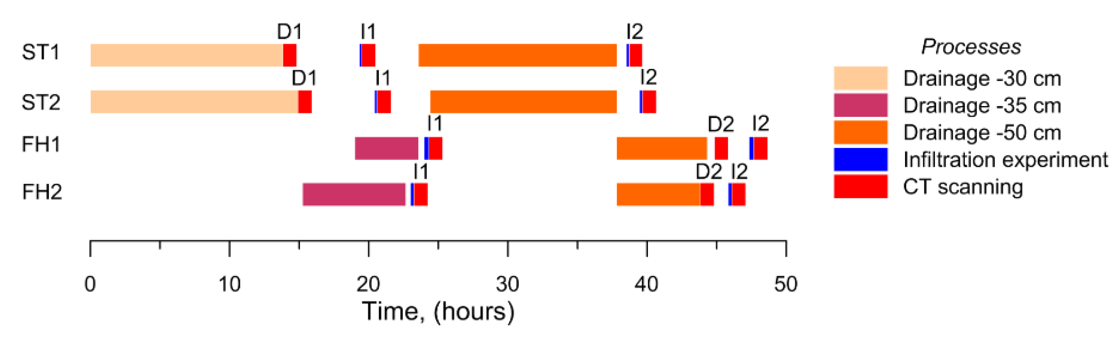
The samples were first fully saturated in a vacuum chamber, after which they were X-rayed while submerged inside the water-filled outer vessel. The samples were then drained at a tension of −30 hPa in the case of material ST and −35 hPa in the case of material FH. The drained ST samples were scanned in air-filled outer vessels. Then an infiltration experiment was applied to all samples followed by immediate imaging. The samples were still submerged inside the water-filled outer vessel during imaging. The second drainage cycle was carried out under a pressure of −50 hPa before a second infiltration run and more X-ray scans were conducted. Details of the experiment schedule are summarized in Table 3 and Figure 4.
2.7. Image Preprocessing
The CT images were preprocessed and analyzed using the software Fiji (ImageJ) [54]. Preprocessing includes the elimination of the noise, edge enhancement and artifact removal [55].
First, all horizontal image layers in the region of interest were selected. The location of the topmost layer depended on the shape of the surface because after the infiltration experiment the surface was not exactly horizontal. The bottommost selected layer was defined by the location of the sample retainer. Then a 3D‑median filter with radius 2 voxels and an unsharp mask was used.
The tomograms were further adjusted to minimize the effect of beam hardening. Beam hardening refers to the non-linear filtering of soft (or low-frequency) X-rays during the beam’s passage through a sample, leaving only harder (or-high-frequency) X-rays in the beam [43]. For soil samples with a cylindrical shape, beam hardening manifests itself as a bright ring artifact along the column’s perimeter [44].
More specifically, the beam-hardening artifacts in this study were detected in two forms: First, along with the entire sample, a general darkening of the image towards the horizontal center of the sand sample. Second, below the PMMA ring, the gray values were attenuated due to the extra X-ray-filtering effect of the ring.
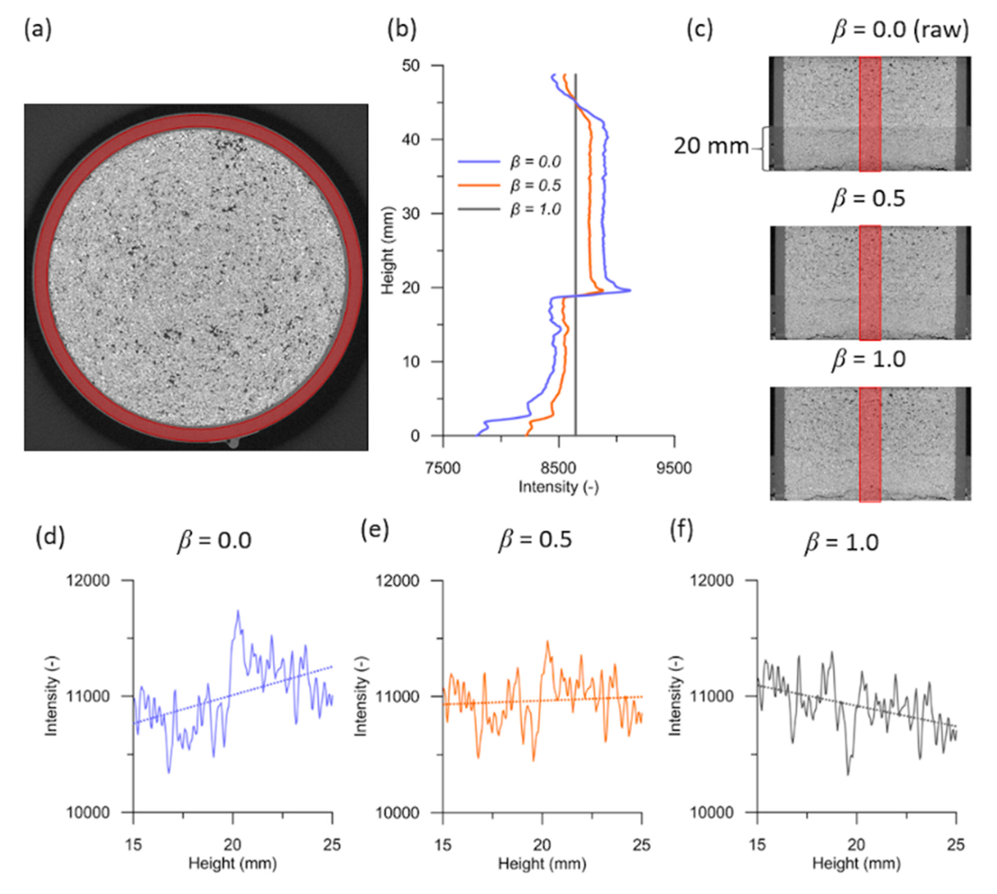
To remove the artifact caused by the PMMA ring, the intensity of each slide was multiplied by a correction coefficient αi. The average image intensity of a 60 pixels wide region of interest located within the wall of the sample cylinder (Figure 5a) was measured for each slice (Ii). The value of correction coefficient αi for the slice i was then:
where Iavg is the average of all the values of Ii and β is a correction factor. The effect of the parameter β on profiles of average image intensity in the central part of the sample (shown in red in Figure 5c) is depicted in Figure 5d–f. A factor of β = 0.5 led to the best correction results.
The next adjustment was related to the second artifact, i.e., the darkening towards the horizontal center of the images. This was done by creating vertical cross-sections through the 3D images. Then, a 9.4 mm (200 pixels) wide strip along the diameter was selected and a profile of intensity was evaluated (Figure 6a,b). This profile was fitted with a center-axis parabola. The ratio between the value on the parabola and the edge values were given by factor ρ. Then each of the images was modified by dividing the intensity by ρ, given the distance from the center of the sample.
2.8. Image Analysis
The images were binarized into two classes—one class depicting the gas phase and the other all other phases, namely the water and solid phases. An automatic binarization was not successful in this case due to poorly recognizable peaks on the intensity histogram. The threshold values were obtained by visual inspection for each sample. Then a morphological opening with a kernel radius of 1 voxel was carried out using the ImageJ plugins 3D Erode and 3D Dilate. We then removed ‘holes’ in the segmented air bubbles, which represented segmentation artifacts, using the 3D Fill Holes plugin [56].
We determined the imaged gas volume content as a function of the height of the sand samples as the ratio between the area of gas and the column cross-section for each image slice. These results were also used to determine the air volume content of the whole sample. The plugin BoneJ [57] was used to evaluate the thickness of the air bubbles, defined as the diameter of the largest sphere that fits within individual bubbles.
3. Results and Discussion
3.1. Initial Gas Saturation
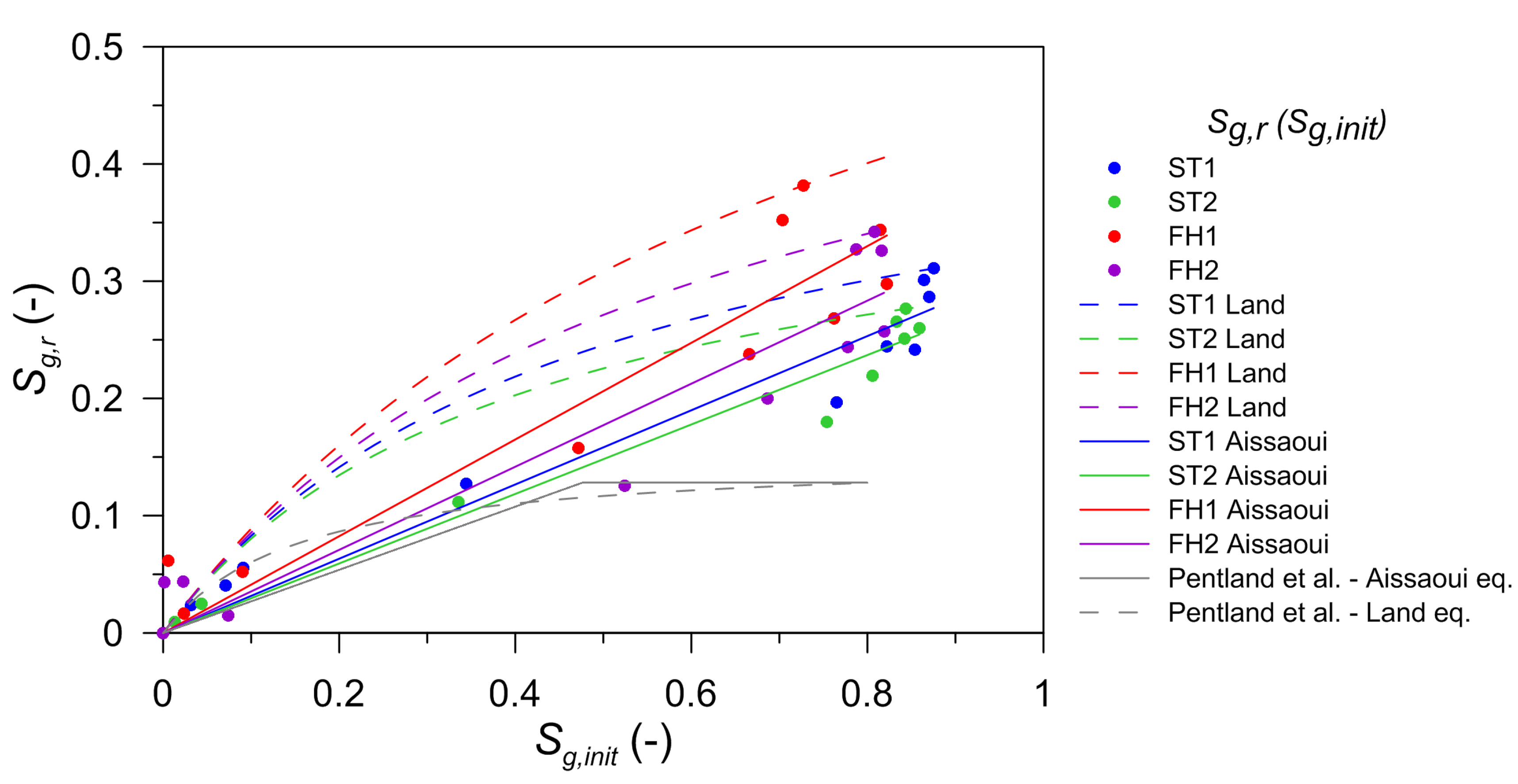
The relationship between initial and residual gas saturation as fitted using Aissaoui’s and Land’s equations is shown in Figure 7 together with the results of Pentland et al. We observed a positive correlation between Sg,init and the residual saturation Sg,r. The maximum of the initial gas saturation ranged between 80% to 90%. The evaluated parameters for Land’s and Aissaoui’s models are shown in Table 4. In our case the growth of Sg,r value did not converge to an upper limit as it was supposed by Aissaoui. On the basis of experiments with octane used as a non-wetting phase, Pentland et al. [53] assumed that the upper limit of Sg,r corresponds to the occupancy of all large pores by the non-wetting phase. They also assumed that small pores continue to fill causing further increase of Sg,init, while Sg,r does not increase, because gas is displaced from the small pores. In our study the upper limit of Sg,r was not detected, probably due to the apparently unstable pore geometry in the upper portion of the sample, where pores enlarged with increasing Sg,init. This effect will be discussed in detail in the next paragraph. Yet, Aissaoui’s equation results in a better fit of the experimental values than the Land’s equation, which is in agreement with Pentland’s study.
3.2. Air Content and Air Distribution
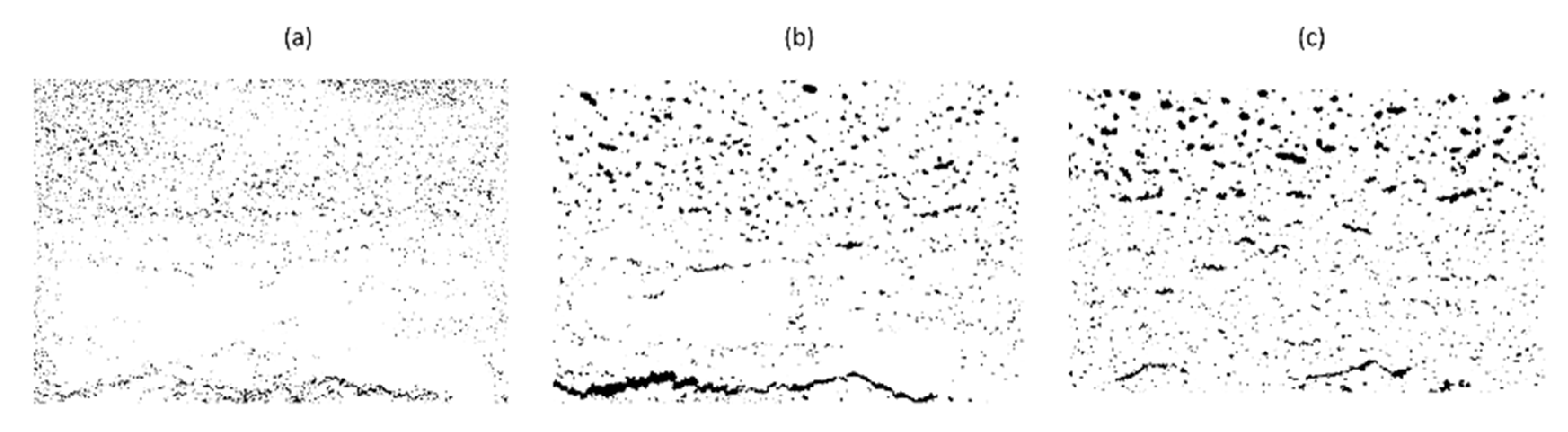
Table 5 lists the volumetric air contents ω of the whole samples, obtained gravimetrically and by X-ray image analysis. The amount of entrapped air, after infiltrations I1 and I2, was higher for FH sand. The values of ω obtained gravimetrically were higher than the values obtained by X-ray imaging. This was probably caused by the fact that bubbles under certain sizes were not detected being below the image resolution. The field of view which determines the image resolution is given by the size of the sample. The size of the sample was designed to be larger than the expected representative elementary volume of sand, which led to an image resolution that neglected the smaller bubbles. Table 5 shows that the gravimetrically measured ω values were significantly larger after drainage than the ω values measured after each infiltration experiment. However, this effect is not reproduced in the X-ray imaging results. On the contrary, we observed the opposite. This could be due to the presence of predominantly small bubbles after drainage that remained too small to be detected in the image data, as can be seen in Figure 8, where vertical cross-sections of the binarized images of the sample ST2 are shown. After drainage (D1) there was a large number of small bubbles, mostly located in the upper half of the sample. We can assume that in this case an additional large number of small bubbles existed, which remained undetected because they were below the resolution of the X-ray images. After the first infiltration experiment (I1), larger pores were created by displacing nearby grains of sand (Figure 8b) and the air had aggregated into larger bubbles, probably due to the effect of Ostwald ripening [58]. After the second infiltration experiment (I2), the bubbles became even larger (Figure 8c). It seems that the higher amount of the visible air bubbles in the sample occurred due to the enlargement of pores.
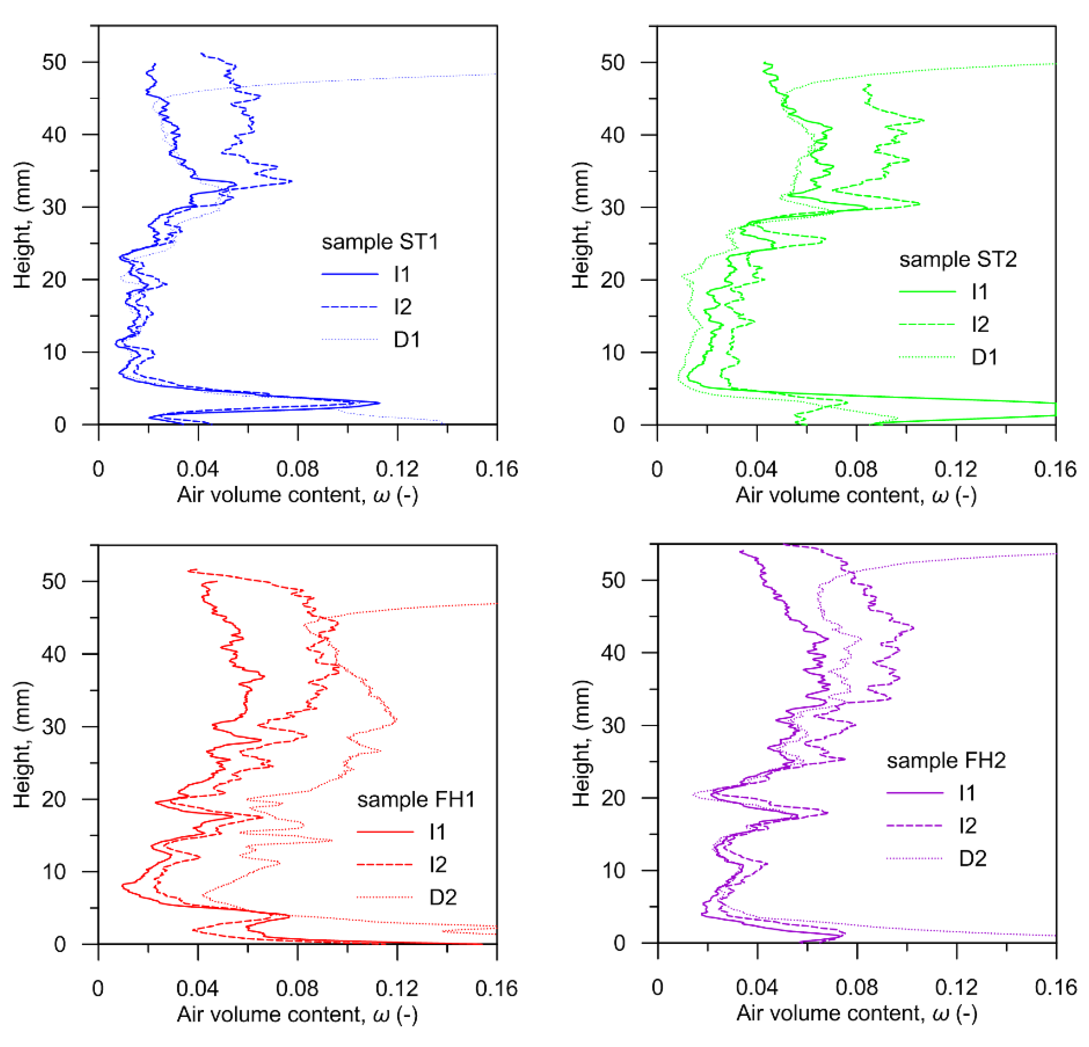
The air saturation profile along the height of the sample is shown in Figure 9. It should be noted that only relatively large bubbles were detected by x-ray CT. It is evident that the air is predominantly distributed in the upper part of the sample, from 25 mm upwards, especially after infiltration experiments (I1, I2). The accumulation of air in large bubbles at the upper half of the sample was probably caused by the buoyancy force in combination with Ostwald ripening.
The amount of air in the upper part is approximately doubled between I1 and I2. The air in the lower 5 mm is predominantly present in newly created cracks.
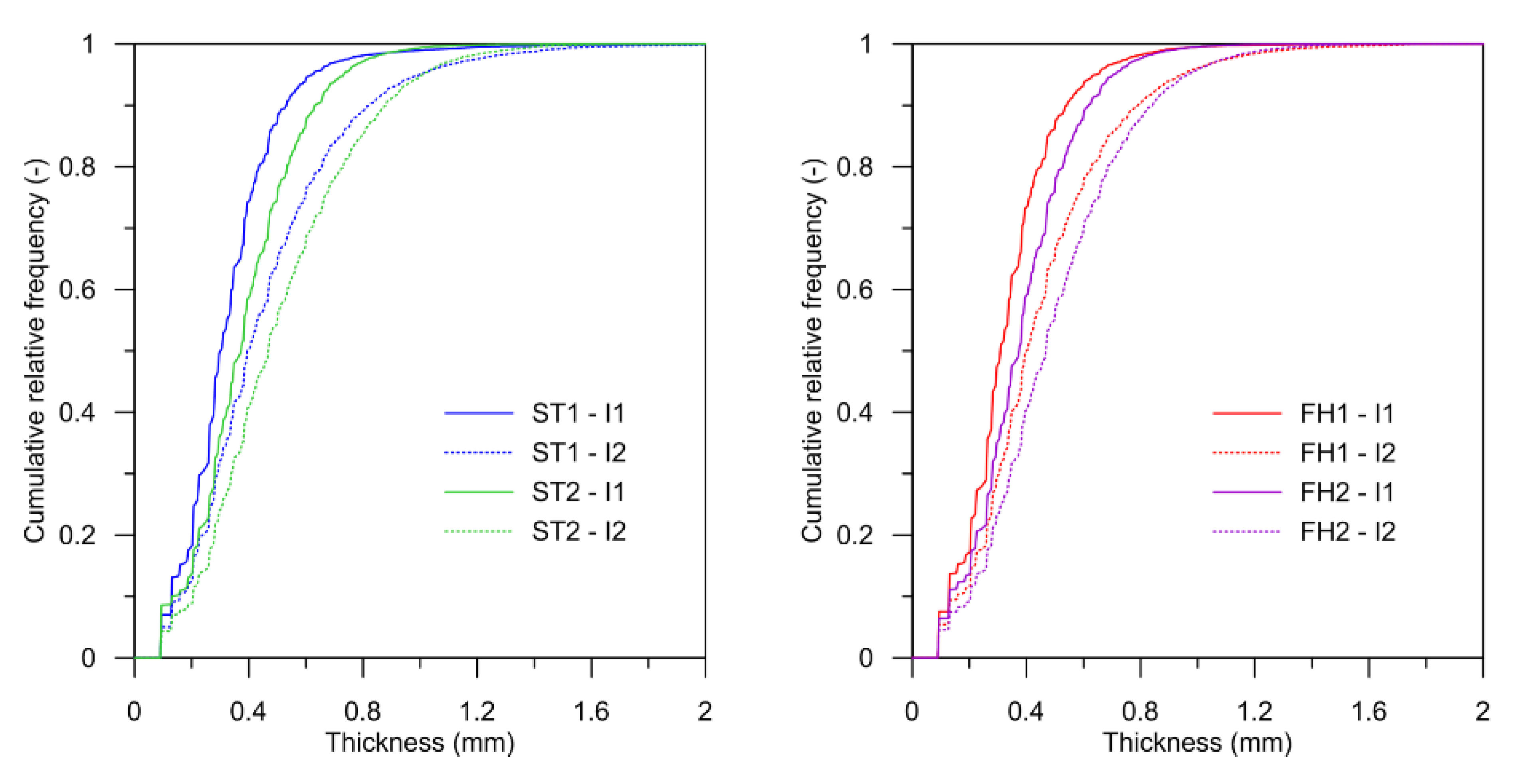
The frequency of the thickness of the bubbles can be seen in Figure 10. To eliminate the effect of the air-filled fractures, only parts of the image 2 cm above the bottom were analyzed. In all the cases, the air bubble thickness increased between stages I1 and I2. More specifically, the thickness of the smallest 50% of the bubbles changed from 300 to 405 µm for ST1, from 370 to 470 µm for ST2, from 310 to 405 µm for FH1, and from 370 to 470 µm for FH2. The maximum thickness of all detected air bubbles was approximately 2000 µm.
3.3. Hydraulic Conductivity
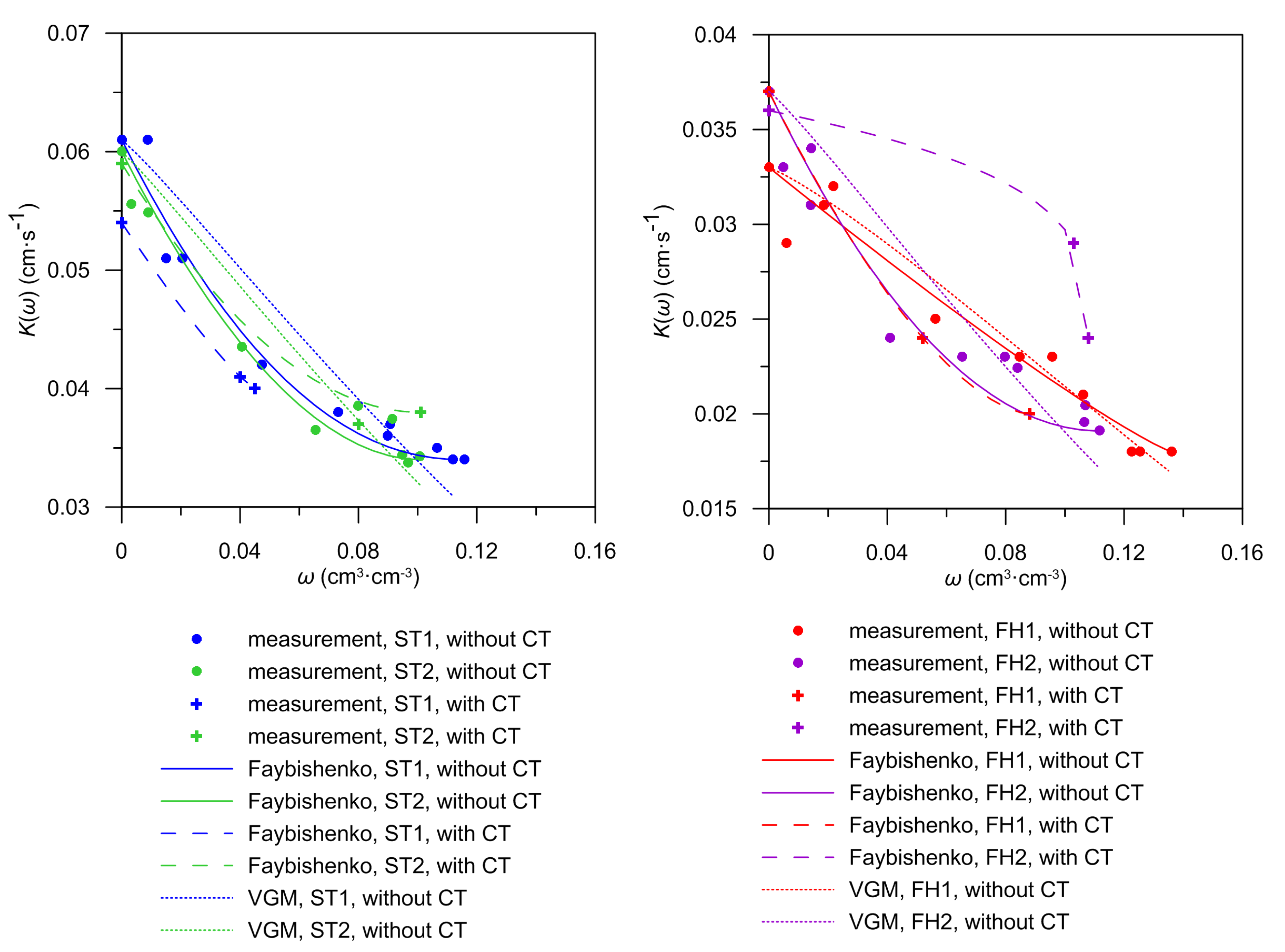
Figure 11 shows the relationship between the satiated hydraulic conductivity and the air content in the sand. Also depicted are fits with Faybishenko’s (2) and VGM functions (3). The respective model parameters n and m were obtained by the least squares method. The corresponding values are shown in Table 6. It can be seen that the results of the infiltration run on the ST samples conducted next to the X-ray scanner followed the same trend as observed for the other 10 experiments. This was not the case for the FH samples, especially not for FH2. One possible explanation could be the smaller number of measured points and the experiment FH2 can be considered as an outlier. The coefficients of determination for both models are given in Table 6. The coefficients of determination for Faybishenko’s model for batch with CT scanning are high due to fitting three points only. KS of the coarser sand ST is almost twice as high as the KS of the finer sand FH. The mean KS of FH sand (0.035 cm·s−1) was similar to the value reported for the same sand FH31 by Sacha et al. (0.040 cm·s−1) and by Haber-Pohlmeier et al. (0.045 cm·s−1) but higher than value given by Sucre et al. (0.011 cm·s−1). Differences between KS values might have been caused by different packing density.
Faybishenko’s model led to similar fits of the K(ω) as the VGM equation. An exception was sample FH1, where the overall shape of the K(ω) was abnormal. In comparison, Marinas et al. [24] determined relatively similar values of coefficients of determination for Faybishenko’s and the VGM equations, with one exception, where Faybishenko’s equation fitted better. The exception was the Unimin-2010 sand, which has a porosity (0.38) and bulk‑density (1.63 g∙cm−3) similar to ST sand. The R2 values for Faybishenko’s equation were 0.952 and 0.927 and R2 values for the VGM equation were 0.890 and 0.841. However, in the VGM equation, Marinas et al. [24] used a fitted exponent l, with values 0.347 and 0.618. In our case, Faybishenko’s parameters n and ωmax are similar to the values published for Masa sandy loam [25].
4. Conclusions
For the purpose of simulation of two-phase flow, the relationship between entrapped air content and satiated hydraulic conductivity K(ω) of two coarse sands was studied. Simultaneously with falling head infiltration and drainage experiments, the X-ray computed tomography imaging was performed to reveal temporal changes of the entrapped air distribution and the bubble shapes within the sample.
The positive correlation between initial air saturation Sg,init and residual air saturation Sg,r was found; this result is in agreement with Land [14] or Mansoori et al. [59]. The maximum value of Sg,r was 0.31 for ST sand and 0.38 for FH sand. A good fit of the Sg,r (Sg,init) relationship was obtained using Aissaoui’s equation.
As expected, the saturated hydraulic conductivity of coarser sand ST was consistently higher than the hydraulic conductivity of finer sand FH. The hydraulic conductivity of samples at full saturation was approximately twice as high as the hydraulic conductivity of samples with maximal entrapped air content. The relationship between air volume content and satiated hydraulic conductivity was successfully fitted with Faybishenko’s equation. Faybishenko’s model seems to be appropriate to express the K(ω) relationship.
X-ray computed tomography revealed that the size of air bubbles and clusters increased significantly with each infiltration-drainage cycle. The final shapes of observed bubbles appeared to be elongated in the horizontal direction. The increase in bubble size was not spatially uniform within an individual sample. Instead, air bubbles grew larger close to the surface of the sample. Bubble ebullition probably also led to the formation of the larger voids in the sand packing.
The obtained K(ω) relationship can be used as a characteristic in newly developed numerical models of two-phase flow, such as the model by Fucik and Mikyska [60]. It is evident that the entrapped air significantly influences measured values of hydraulic conductivity even in samples of simple material and geometry. The presented methodology can be used to determine the K(ω) in other natural and artificial porous materials.
Author Contributions
T.P. and H.M.R.F. conducted the experiments and wrote an original draft. T.P. did the development of methodology and formal analysis of results. J.K. provisioned CT imaging of sand samples, contributed to the image analysis and reviewed and edited the manuscript. M.S. did conceptualization, funding acquisition, project administration and supervision, development of methodology and review and editing of the manuscript. All authors have read and agreed to the published version of the manuscript.
Funding
This research was funded by the Czech Science Foundation under project number GA17-06759S and by the Grant Agency of the Czech Technical University in Prague, grant No. SGS18/122/OHK1/2T/11.
Acknowledgments
We thank Milena Cislerova for valuable comments that greatly improved the manuscript.
Conflicts of Interest
The authors declare no conflict of interest.
Appendix A
The initial gas saturation (Sg,init) value determines the amount of gas that is in the sample after drainage in a sand box. The mass of the sample container with sand after drainage (when the sample was not yet submerged in water) is Msamp,init. To evaluate Sg,init, also the value of the mass of the sample container with sand after the full saturation, Msamp,sat, must be acquired. The difference between Msamp,sat and Msamp,init determines the mass of water that has been replaced by gas and thus the volume of entrapped gas within the sand sample (assuming ρw =1 g∙cm−3). Sg,init value is then:
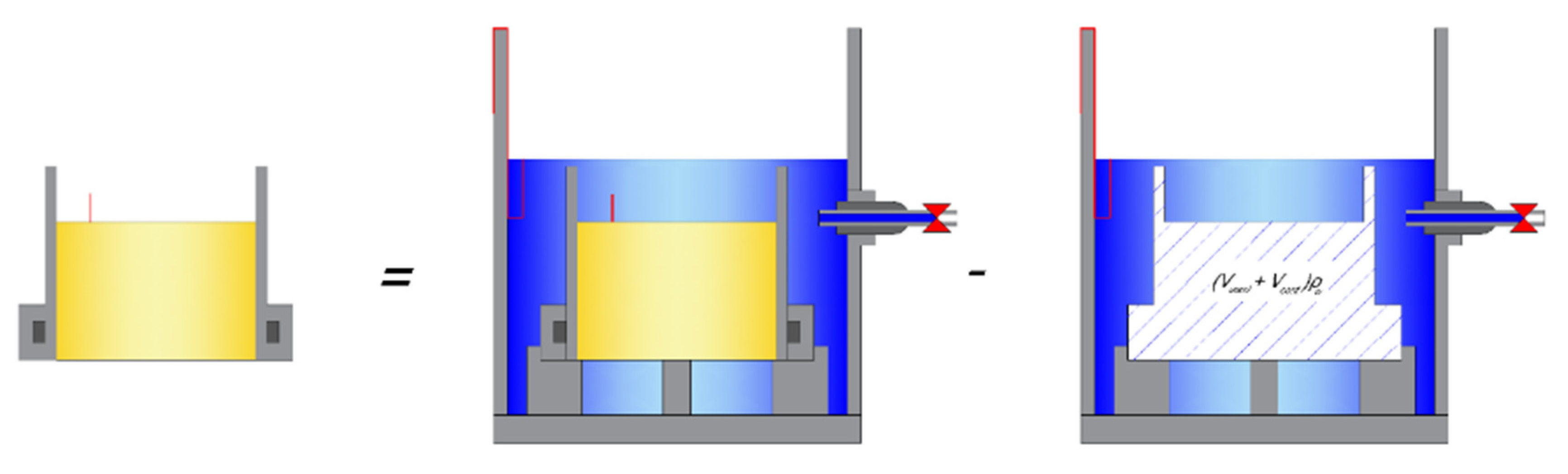
where ρw is water density and p is the porosity of the sand sample. The mass of the fully saturated sample (see Figure A1) Msamp,sat is:
where M0 is the mass of the outer vessel with a fully saturated sample (see Figure 3c), Mfill,w is the mass of the vessel without the sample, when the water level is exactly at the reference level. Vsand is the volume of the sand sample, Vcont is the volume of the container wall and ring.
Figure A1.
Mass of the saturated sand sample and sample container (Msamp,sat) is equal to the difference between the mass of the vessel with fully saturated sample flooded to the reference level (M0) and the mass of the vessel and water surrounding sample (Mfill,w – (Vsand+Vcont)ρw).
Figure A1.
Mass of the saturated sand sample and sample container (Msamp,sat) is equal to the difference between the mass of the vessel with fully saturated sample flooded to the reference level (M0) and the mass of the vessel and water surrounding sample (Mfill,w – (Vsand+Vcont)ρw).

References
- Faybishenko, B. Hydraulic behavior of quasi-saturated soils in the presence of entrapped air - laboratory experiments. Water Resour. Res. 1995, 31, 2421–2435. [Google Scholar] [CrossRef]
- Sacha, J.; Jelinkova, V.; Snehota, M.; Vontobel, P.; Hovind, J.; Cislerova, M. Water and air redistribution within a dual permeability porous system investigated using neutron imaging. Proc. 10th World Conf. Neutron Radiogr. (Wcnr-10) 2015, 69, 530–536. [Google Scholar] [CrossRef] [Green Version]
- Snehota, M.; Jelinkova, V.; Sobotkova, M.; Sacha, J.; Vontobel, P.; Hovind, J. Water and entrapped air redistribution in heterogeneous sand sample: Quantitative neutron imaging of the process. Water Resour. Res. 2015, 51, 1359–1371. [Google Scholar] [CrossRef] [Green Version]
- Roy, J.W.; Smith, J.E. Multiphase flow and transport caused by spontaneous gas phase growth in the presence of dense non-aqueous phase liquid. J. Contam. Hydrol. 2007, 89, 251–269. [Google Scholar] [CrossRef] [PubMed]
- Tzimas, G.C.; Matsuura, T.; Avraam, D.G.; VanderBrugghen, W.; Constantinides, G.N.; Payatakes, A.C. The combined effect of the viscosity ratio and the wettability during forced imbibition through nonplanar porous media. J. Colloid Interface Sci. 1997, 189, 27–36. [Google Scholar] [CrossRef]
- Ausweger, G.M.; Schweiger, H.F. Numerical study on the influence of entrapped air bubbles on the time-dependent pore pressure distribution in soils due to external changes in water level. In Proceedings of the 3rd European Conference on Unsaturated Soils (E-UNSAT), Paris, France, 12–14 September 2016. [Google Scholar]
- Boulding, J.R.; Ginn, S.J. Practical Handbook of Soil, Vadose Zone, and Ground-Water Contamination: Assessment, Prevention, and Remediation, Second Edition; CRC Press: Boca Raton, FL, USA, 2003. [Google Scholar]
- Chatzis, I.; Morrow, N.R.; Lim, H.T. Magnitude and detailed structure of residual oil saturation. Soc. Pet. Eng. J. 1983, 23, 311–326. [Google Scholar] [CrossRef]
- Almajid, M.M.; Kovscek, A.R. Pore-level mechanics of foam generation and coalescence in the presence of oil. Adv. Colloid Interface Sci. 2016, 233, 65–82. [Google Scholar] [CrossRef]
- Kovscek, A.R.; Tang, G.Q.; Radke, C.J. Verification of Roof snap off as a foam-generation mechanism in porous media at steady state. Colloids Surf. A-Phys. Eng. Asp. 2007, 302, 251–260. [Google Scholar] [CrossRef]
- Cislerova, M.; Simunek, J.; Vogel, T. Changes of steady-state infiltration rates in recurrent ponding infiltration experiments. J. Hydrol. 1988, 104, 1–16. [Google Scholar] [CrossRef]
- Li, Y.; Flores, G.; Xu, J.; Yue, W.Z.; Wang, Y.X.; Luan, T.G.; Gu, Q.B. Residual air saturation changes during consecutive drainage-imbibition cycles in an air-water fine sandy medium. J. Hydrol. 2013, 503, 77–88. [Google Scholar] [CrossRef]
- Nguyen, V.H.; Sheppard, A.P.; Knackstedt, M.A.; Pinczewski, W.V. The effect of displacement rate on imbibition relative permeability and residual saturation. J. Pet. Sci. Eng. 2006, 52, 54–70. [Google Scholar] [CrossRef]
- Land, C.S. Calculation of imbibition relative permeability for two and three-phase flow from rock properties. Soc. Pet. Eng. J. 1968, 8, 149. [Google Scholar] [CrossRef]
- Krol, M.M.; Mumford, K.G.; Johnson, R.L.; Sleep, B.E. Modeling discrete gas bubble formation and mobilization during subsurface heating of contaminated zones. Adv. Water Resour. 2011, 34, 537–549. [Google Scholar] [CrossRef]
- Bear, J. Dynamics of Fluids in Porous Media; Elsevier: New York, NY, USA, 1972. [Google Scholar]
- Hilfer, R. Capillary pressure, hysteresis and residual saturation in porous media. Phys. A-Stat. Mech. Its Appl. 2006, 359, 119–128. [Google Scholar] [CrossRef]
- Mualem, Y. New model for predicting hydraulic conductivity of unsaturated porous-media. Water Resour. Res. 1976, 12, 513–522. [Google Scholar] [CrossRef] [Green Version]
- Childs, E.C.; Collisgeorge, N. The permeability of porous materials. Proc. R. Soc. Lond. Ser. A-Math. Phys. Sci. 1950, 201, 392–405. [Google Scholar] [CrossRef] [Green Version]
- Brooks, R.H.; Corey, A.T. Hydraulic Properties of Porous Media, 3rd ed.; Colorado State University: Fort Collins, CO, USA, 1964. [Google Scholar]
- Van Genuchten, M.T. A closed-form equation for predicting the hydraulic conductivity of unsaturated soils. Soil Sci. Soc. Am. J. 1980, 44, 892–898. [Google Scholar] [CrossRef] [Green Version]
- Fry, V.A.; Selker, J.S.; Gorelick, S.M. Experimental investigations for trapping oxygen gas in saturated porous media for in situ bioremediation. Water Resour. Res. 1997, 33, 2687–2696. [Google Scholar] [CrossRef] [Green Version]
- Ryan, M.C.; MacQuarrie, K.T.B.; Harman, J.; McLellan, J. Field and modeling evidence for a "stagnant flow" zone in the upper meter of sandy phreatic aquifers. J. Hydrol. 2000, 233, 223–240. [Google Scholar] [CrossRef]
- Marinas, M.; Roy, J.W.; Smith, J.E. Changes in Entrapped Gas Content and Hydraulic Conductivity with Pressure. Ground Water 2013, 51, 41–50. [Google Scholar] [CrossRef]
- Sakaguchi, A.; Nishimura, T.; Kato, M. The effect of entrapped air on the quasi-saturated soil hydraulic conductivity and comparison with the unsaturated hydraulic conductivity. Vadose Zone J. 2005, 4, 139–144. [Google Scholar] [CrossRef]
- Loizeau, S.; Rossier, Y.; Gaudet, J.P.; Refloch, A.; Besnard, K.; Angulo-Jaramillo, R.; Lassabatere, L. Water infiltration in an aquifer recharge basin affected by temperature and air entrapment. J. Hydrol. Hydromech. 2017, 65, 222–233. [Google Scholar] [CrossRef] [Green Version]
- Pohlmeier, A.; Garre, S.; Roose, T. Noninvasive Imaging of Processes in Natural Porous Media: From Pore to Field Scale. Vadose Zone J. 2018, 17. [Google Scholar] [CrossRef]
- Yu, X.; Hong, C.; Peng, G.; Lu, S. Response of pore structures to long-term fertilization by a combination of synchrotron radiation X-ray microcomputed tomography and a pore network model. Eur. J. Soil Sci. 2018, 69, 290–302. [Google Scholar] [CrossRef]
- Udawatta, R.P.; Gantzer, C.J.; Anderson, S.H.; Assouline, S. Synchrotron microtomographic quantification of geometrical soil pore characteristics affected by compaction. Soil 2016, 2, 211–220. [Google Scholar] [CrossRef]
- Zong, Y.T.; Yu, X.L.; Zhu, M.X.; Lu, S.G. Characterizing soil pore structure using nitrogen adsorption, mercury intrusion porosimetry, and synchrotron-radiation-based X-ray computed microtomography techniques. J. Soils Sediments 2015, 15, 302–312. [Google Scholar] [CrossRef]
- Peth, S.; Horn, R.; Beckmann, F.; Donath, T.; Fischer, J.; Smucker, A.J.M. Three-dimensional quantification of intra-aggregate pore-space features using synchrotron-radiation-based microtomography. Soil Sci. Soc. Am. J. 2008, 72, 897–907. [Google Scholar] [CrossRef]
- Zhou, H.; Peng, X.; Peth, S.; Xiao, T.Q. Effects of vegetation restoration on soil aggregate microstructure quantified with synchrotron-based micro-computed tomography. Soil Tillage Res. 2012, 124, 17–23. [Google Scholar] [CrossRef]
- Ma, R.M.; Cai, C.F.; Li, Z.X.; Wang, J.G.; Xiao, T.Q.; Peng, G.Y.; Yang, W. Evaluation of soil aggregate microstructure and stability under wetting and drying cycles in two Ultisols using synchrotron-based X-ray micro-computed tomography. Soil Tillage Res. 2015, 149, 1–11. [Google Scholar] [CrossRef]
- Wildenschild, D.; Hopmans, J.W.; Rivers, M.L.; Kent, A.J.R. Quantitative analysis of flow processes in a sand using synchrotron-based X-ray microtomography. Vadose Zone J. 2005, 4, 112–126. [Google Scholar] [CrossRef]
- Schnaar, G.; Brusseau, M.L. Characterizing pore-scale configuration of organic immiscible liquid in multiphase systems with synchrotron X-ray microtomography. Vadose Zone J. 2006, 5, 641–648. [Google Scholar] [CrossRef] [Green Version]
- Koestel, J.; Schluter, S. Quantification of the structure evolution in a garden soil over the course of two years. Geoderma 2019, 338, 597–609. [Google Scholar] [CrossRef]
- Sandin, M.; Koestel, J.; Jarvis, N.; Larsbo, M. Post-tillage evolution of structural pore space and saturated and near-saturated hydraulic conductivity in a clay loam soil. Soil Tillage Res. 2017, 165, 161–168. [Google Scholar] [CrossRef]
- Suekane, T.; Thanh, N.H.; Matsumoto, T.; Matsuda, M.; Kiyota, M.; Ousaka, A. Direct measurement of trapped gas bubbles by capillarity on the pore scale. Greenh. Gas Control Technol. 9 2009, 1, 3189–3196. [Google Scholar] [CrossRef] [Green Version]
- Setiawan, A.; Nomura, H.; Suekane, T. Microtomography of Imbibition Phenomena and Trapping Mechanism. Transp. Porous Media 2012, 92, 243–257. [Google Scholar] [CrossRef]
- Geistlinger, H.; Mohammadian, S.; Schlueter, S.; Vogel, H.J. Quantification of capillary trapping of gas clusters using X-ray microtomography. Water Resour. Res. 2014, 50, 4514–4529. [Google Scholar] [CrossRef]
- Geistlinger, H.; Mohammadian, S. Capillary trapping mechanism in strongly water wet systems: Comparison between experiment and percolation theory. Adv. Water Resour. 2015, 79, 35–50. [Google Scholar] [CrossRef]
- Herring, A.L.; Gilby, F.J.; Li, Z.; McClure, J.E.; Turner, M.; Veldkamp, J.P.; Beeching, L.; Sheppard, A.P. Observations of nonwetting phase snap-offduring drainage. Adv. Water Resour. 2018, 121, 32–43. [Google Scholar] [CrossRef]
- Barrett, J.F.; Keat, N. Artifacts in CT: Recognition and avoidance. Radiographics 2004, 24, 1679–1691. [Google Scholar] [CrossRef]
- Weller, U.; Leuther, F.; Schluter, S.; Vogel, H.J. Quantitative Analysis of Water Infiltration in Soil Cores Using X-Ray. Vadose Zone J. 2018, 17. [Google Scholar] [CrossRef] [Green Version]
- Izadi, B.; Podmore, T.H.; Seymour, R.M. Consideration of air entrapment in surface irrigation - a computer-simulation study. Agric. Water Manag. 1995, 28, 245–252. [Google Scholar] [CrossRef]
- Goncalves, R.D.; Teramoto, E.H.; Engelbrecht, B.Z.; Alfaro Soto, M.A.; Chang, H.K.; van Genuchten, M.T. Quasi-Saturated Layer: Implications for Estimating Recharge and Groundwater Modeling. Groundwater 2019. [Google Scholar] [CrossRef]
- Mizrahi, G.; Furman, A.; Weisbrod, N. Infiltration under Confined Air Conditions: Impact of Inclined Soil Surface. Vadose Zone J. 2016, 15. [Google Scholar] [CrossRef]
- Sacha, J.; Snehota, M.; Trtik, P.; Hovind, J. Impact of Infiltration Rate on Residual Air Distribution and Hydraulic Conductivity. Vadose Zone J. 2019, 18. [Google Scholar] [CrossRef] [Green Version]
- Klute, A. Water retention: Laboratory methods. In Methods of Soil Analysis—Part 1—Physical and Mineralogical Methods; Klute, A., Ed.; American Society of Agronomy: Madison, WI, USA, 1986; pp. 635–662. [Google Scholar]
- Klute, A.; Dirksen, C. Hydraulic conductivity and diffusivity: Laboratory methods. In Methods of Soil Analysis—Part 1—Physical and Mineralogical Methods; Klute, A., Ed.; American Society of Agronomy: Madison, WI, USA, 1986; pp. 687–734. [Google Scholar]
- Averyanov, S.F. Zavisimost vodopronitsaemosti pochvo-gruntov ot soderzhaniya v nikh vozdukha. Dokl. Akad. Nauk Sssr 1949, 69, 141–144. [Google Scholar]
- Aissaoui, A. Etude théorique et expérimentale de l'hystérésis despressions capillaries et des perméabilitiés relatives en vue du stockagesouterrain de gaz. Ph.D. Thesis, École des Mines de Paris, Paris, France, 1983. [Google Scholar]
- Pentland, C.H.; Itsekiri, E.; Al Mansoori, S.K.; Iglauer, S.; Bijeljic, B.; Blunt, M.J. Measurement of Nonwetting-Phase Trapping in Sandpacks. Spe J. 2010, 15, 274–281. [Google Scholar] [CrossRef] [Green Version]
- Schindelin, J.; Arganda-Carreras, I.; Frise, E.; Kaynig, V.; Longair, M.; Pietzsch, T.; Preibisch, S.; Rueden, C.; Saalfeld, S.; Schmid, B.; et al. Fiji: An open-source platform for biological-image analysis. Nat. Methods 2012, 9, 676–682. [Google Scholar] [CrossRef] [PubMed] [Green Version]
- Schluter, S.; Sheppard, A.; Brown, K.; Wildenschild, D. Image processing of multiphase images obtained via X- ray microtomography: A review. Water Resour. Res. 2014, 50, 3615–3639. [Google Scholar] [CrossRef]
- Ollion, J.; Cochennec, J.; Loll, F.; Escude, C.; Boudier, T. TANGO: A generic tool for high-throughput 3D image analysis for studying nuclear organization. Bioinformatics 2013, 29, 1840–1841. [Google Scholar] [CrossRef]
- Doube, M.; Klosowski, M.M.; Arganda-Carreras, I.; Cordelieres, F.P.; Dougherty, R.P.; Jackson, J.S.; Schmid, B.; Hutchinson, J.R.; Shefelbine, S.J. BoneJ Free and extensible bone image analysis in ImageJ. Bone 2010, 47, 1076–1079. [Google Scholar] [CrossRef] [Green Version]
- Garing, C.; de Chalendar, J.A.; Voltolini, M.; Ajo-Franklin, J.B.; Benson, S.M. Pore-scale capillary pressure analysis using multi-scale X-ray micromotography. Adv. Water Resour. 2017, 104, 223–241. [Google Scholar] [CrossRef] [Green Version]
- Al Mansoori, S.; Iglauer, S.; Pentland, C.H.; Bijeljic, B.; Blunt, M.J. Measurements of Non-Wetting Phase Trapping Applied to Carbon Dioxide Storage. Greenh. Gas Control Technol. 9 2009, 1, 3173–3180. [Google Scholar] [CrossRef] [Green Version]
- Fucik, R.; Mikyska, J. Mixed-hybrid finite element method for modelling two-phase flow in porous media. J. Math. Ind. 2011, 3, 9–19. [Google Scholar]
Figure 1.
Grain-size distribution of the sands under study.

Figure 2.
Schema of the experimental setup. Left: The sample container filled with sand and inserted into the outer vessel. The peristaltic pump is connected to the overflow. Right: The sample container and the retainers in detail and with dimensions.
Figure 2.
Schema of the experimental setup. Left: The sample container filled with sand and inserted into the outer vessel. The peristaltic pump is connected to the overflow. Right: The sample container and the retainers in detail and with dimensions.

Figure 3.
Illustration of the infiltration experiment for measurements of KS: (a) The saturation of the sand sample in the vacuum chamber. The valve is closed; (b) the ponding infiltration experiment: L is the height of the sample and ΔH is the difference of hydraulic heads. The valve is opened, and the peristaltic pump keeps the lower water level in the outer vessel constant. When the water level on the sand sample drops to the tip of the pin, another batch of 40 cm3 of water is poured. This is repeated at least 15 times; (c) the sample is prepared for weighing.

Figure 4.
Schedule of the experiment with X-ray micro-tomography imaging. CT imaging (shown in red color) was conducted after the first infiltration (I1) and after the second infiltration (I2). CT imaging was also performed after drainage (D1 and D2) experiment and character D indicates CT scanning after drainage. The duration of scan was 1 hour and duration of infiltration experiment was from 10 to 20 minutes.

Figure 5.
Adjustment of the vertical beam hardening artifact: (a) Slice with marked ROI corresponding to sample wall; (b) Profile of the Ii (average image intensity inside the wall in particular slice) for different values of β; (c) visual comparison for adjustments with different values of β. Note, that lower 20 mm are affected by the presence of the ring; (d–f) details of the image intensity inside the sand for the region most affected by the artefact.

Figure 6.
Adjustment of the cupping artifact: (a) Marked ROI; (b) course of the intensity in ROI from Figure 6a before and after adjustment; (c) image before the adjustment; (d) image after the adjustment.
Figure 6.
Adjustment of the cupping artifact: (a) Marked ROI; (b) course of the intensity in ROI from Figure 6a before and after adjustment; (c) image before the adjustment; (d) image after the adjustment.

Figure 7.
Initial gas saturation vs. residual gas saturation, for experiment without CT. The modified Land’s (5) and Aissaoui’s (6) equations were used for fitting. Pentland et al. [53] used octane in a sandpack.
Figure 7.
Initial gas saturation vs. residual gas saturation, for experiment without CT. The modified Land’s (5) and Aissaoui’s (6) equations were used for fitting. Pentland et al. [53] used octane in a sandpack.

Figure 8.
Differences between gas bubbles distribution and bubbles sizes in sample ST2 in different stages: (a) stage D1; (b) stage I1; (c) stage I2. In the figure are the vertical cross-sections through the center.
Figure 8.
Differences between gas bubbles distribution and bubbles sizes in sample ST2 in different stages: (a) stage D1; (b) stage I1; (c) stage I2. In the figure are the vertical cross-sections through the center.

Figure 9.
Air volume content of the sand as a function of the height.

Figure 10.
Bubble thickness for the stages after the infiltration experiment (I1 and I2).

Figure 11.
Satiated hydraulic conductivity of sands as a function of entrapped air content, fitted by Faybishenko’s and Mualem’s (VGM) models (lines). The ST sand is on left and FH sand is on right.
Figure 11.
Satiated hydraulic conductivity of sands as a function of entrapped air content, fitted by Faybishenko’s and Mualem’s (VGM) models (lines). The ST sand is on left and FH sand is on right.


Table 1.
Characteristics of sand samples.
| Sand Sample | Dry Bulk Density (g∙cm−3) | Porosity (−) | Height (cm) | Volume (cm3) |
|---|---|---|---|---|
| ST1 | 1.66 | 0.372 | 5.1 | 207.6 |
| ST2 | 1.68 | 0.364 | 5.1 | 207.6 |
| FH1 | 1.71 | 0.357 | 5.2 | 211.7 |
| FH2 | 1.78 | 0.327 | 5.5 | 223.9 |
Table 2.
Pressure heads set on sand box and duration of drainage runs for samples ST and FH.
| Run No. | 1 | 2 | 3 | 4 | 5 | 6 | 7 | 8 | 9 | 10 |
|---|---|---|---|---|---|---|---|---|---|---|
| Pressure Head (cm) | −4 | −10 | −20 | −30 | −35 | −40 | −50 | −50 | −50 | −50 |
| Duration (h) | 21 | 23 | 22 | 21 | 20 | 20 | 17 | 20 | 24 | 24 |
Table 3.
Pressure heads set on a sand box in the experiment with computed micro-tomography (CT) imaging of the sample.
Table 3.
Pressure heads set on a sand box in the experiment with computed micro-tomography (CT) imaging of the sample.
| Parameters of Drainage | ST1 | ST2 | FH1 | FH2 |
|---|---|---|---|---|
| Pressure Head (cm) | −30 | −30 | −35 | −35 |
| Duration (h) | 14 | 15 | 4.5 | 7.5 |
| Pressure Head (cm) | −50 | −50 | −50 | −50 |
| Duration (h) | 14 | 13 | 6.5 | 6.0 |
Table 4.
Values of the parameters and coefficients of determination for Land’s equation (5) and Aissaoui’s equation (6).
Table 4.
Values of the parameters and coefficients of determination for Land’s equation (5) and Aissaoui’s equation (6).
| Sand Sample | Land | Aissaoui | |||
|---|---|---|---|---|---|
| Sg,r,max | Sg,init,max | R2 | Sg,r,max | R2 | |
| ST1 | 0.311 | 0.875 | 0.9183 | 0.311 | 0.9531 |
| ST2 | 0.276 | 0.843 | 0.9149 | 0.276 | 0.9682 |
| FH1 | 0.382 | 0.727 | 0.8570 | 0.382 | 0.9002 |
| FH2 | 0.342 | 0.808 | 0.8101 | 0.342 | 0.9019 |
Table 5.
Comparison of values of the air volume content obtained by gravimetric method and image analysis.
Table 5.
Comparison of values of the air volume content obtained by gravimetric method and image analysis.
| Property | Experiment Stage | ST1 | ST2 | FH1 | FH2 |
|---|---|---|---|---|---|
| Porosity (–) | - | 0.372 | 0.364 | 0.357 | 0.327 |
| ω gravimetric (–) | D1 | 0.244 | 0.140 | 0.175 | 0.197 |
| I1 | 0.040 | 0.080 | 0.051 | 0.103 | |
| D2 | 0.300 | 0.300 | 0.283 | 0.252 | |
| I2 | 0.045 | 0.101 | 0.088 | 0.108 | |
| ω image analysis (–) | D1 | 0.035 | 0.040 | - | - |
| I1 | 0.026 | 0.044 | 0.046 | 0.045 | |
| D2 | - | - | 0.055 | 0.056 | |
| I2 | 0.039 | 0.059 | 0.063 | 0.065 |
Table 6.
Parameters and coefficients of determination of Faybishenko´s and VGM model.
| Parameters of Models | ST1 | ST2 | FH1 | FH2 |
|---|---|---|---|---|
| Without CT—Faybishenko | ||||
| n (−) | 2.13 | 1.90 | 1.14 | 2.00 |
| K0 (cm∙s−1) | 0.034 | 0.034 | 0.018 | 0.019 |
| KS (cm∙s−1) | 0.061 | 0.060 | 0.033 | 0.037 |
| ωmax (−) | 0.116 | 0.107 | 0.142 | 0.117 |
| R2 | 0.9694 | 0.9665 | 0.9448 | 0.9327 |
| Without CT—VGM | ||||
| m (−) | 1.15 | 1.13 | 1.36 | 1.17 |
| R2 | 0.8701 | 0.9055 | 0.9382 | 0.8178 |
| With CT—Faybishenko | ||||
| n (−) | 1.20 | 1.97 | 1.62 | 0.28 |
| K0 (cm∙s−1) | 0.040 | 0.038 | 0.020 | 0.024 |
| KS (cm∙s−1) | 0.054 | 0.059 | 0.037 | 0.036 |
| ωmax (−) | 0.045 | 0.101 | 0.088 | 0.108 |
| R2 | 1.0000 | 0.9877 | 1.0000 | 1.0000 |
© 2020 by the authors. Licensee MDPI, Basel, Switzerland. This article is an open access article distributed under the terms and conditions of the Creative Commons Attribution (CC BY) license (http://creativecommons.org/licenses/by/4.0/).
Share and Cite
MDPI and ACS Style
Princ, T.; Fideles, H.M.R.; Koestel, J.; Snehota, M. The Impact of Capillary Trapping of Air on Satiated Hydraulic Conductivity of Sands Interpreted by X-ray Microtomography. Water 2020, 12, 445. https://doi.org/10.3390/w12020445
AMA Style
Princ T, Fideles HMR, Koestel J, Snehota M. The Impact of Capillary Trapping of Air on Satiated Hydraulic Conductivity of Sands Interpreted by X-ray Microtomography. Water. 2020; 12(2):445. https://doi.org/10.3390/w12020445
Chicago/Turabian StylePrinc, Tomas, Helena Maria Reis Fideles, Johannes Koestel, and Michal Snehota. 2020. "The Impact of Capillary Trapping of Air on Satiated Hydraulic Conductivity of Sands Interpreted by X-ray Microtomography" Water 12, no. 2: 445. https://doi.org/10.3390/w12020445
Note that from the first issue of 2016, this journal uses article numbers instead of page numbers. See further details here.