Forcing for a Cascaded Lattice Boltzmann Shallow Water Model

Abstract

This work compares three forcing schemes for a recently introduced cascaded lattice Boltzmann shallow water model: a basic scheme, a second-order scheme, and a centred scheme. Although the force is applied in the streaming step of the lattice Boltzmann model, the acceleration is also considered in the transformation to central moments. The model performance is tested for one and two dimensional benchmarks.

1. Introduction

We present a multi-relaxation times (MRT) lattice Boltzmann cascaded collision operator (CO), based on central moments, and its application to shallow water flows. The method used here is the cascaded lattice Boltzmann shallow water model, partially described in [1], where the link between central moments and cumulants is underlined in the implementation procedure of the cumulant collision operator. Our focus is on the inclusion of forcing schemes for the modeling of gravity in an environment of non-flat seabeds. The shallow water equations (SWE) allow to simulate flows in water bodies where the horizontal length scale is much larger than the fluid depth. The SWE are derived from the three dimensional incompressible Navier–Stokes equations using an integration over the depth to obtain vertically averaged quantities. They are valid for problems in which the vertical dynamics of the fluid can be neglected [2]. The pressure distribution in the vertical direction z, $p^{}\left(z\right)$, is supposed to be hydrostatic. A system of 2D shallow water equations can be written in the following form [3]:

$$\frac{\partial h^{}}{\partial t}+\frac{\partial \left(h^{}{u}_j^{}\right)}{\partial x_j}=0$$

(1)

$$u_j^{}=\frac{1}{h}{\int }_{z_b^{}}^{z_b^{}+h^{}}{u}^{}dz$$

(2)

$$\frac{\partial \left(h^{}{u}_i^{}\right)}{\partial t}+\frac{\partial \left(h^{}{u^{}}_i{u^{}}_j\right)}{\partial x_j}=-g^{}\frac{\partial }{\partial x_i}\left(\frac{{h^{}}^2}{2}\right)+{\nu }^{}\frac{{\partial }^2\left(h^{}{u^{}}_i\right)}{\partial x_j\partial x_j}+F_i^{}$$

(3)

where i and j indicate the coordinate axis direction in 2D space, $h^{}$ is the water depth, $u^{}$ is the velocity, ${\nu }^{}$ is the kinematic viscosity, $z_b$ is the bed elevation, and $F_i^{}$ is the external force in the i direction. If vertical variations must be taken into account, these can be separated from the horizontal ones using a set of shallow water equations for each horizontal fluid layers (multilayer SWE) [4]. The SWE is used in ocean engineering [5], hydraulic engineering [6,7], and coastal engineering [8]. They allow to study a wide range of physical problems such as storm surges, tidal flows and fluctuations in estuary and coastal water regions, tsunami, stationary hydraulic jumps, off-shore structures, and open channel flows. Moreover, the SWE can also be coupled to transport equations to model the conveyance of several quantities such as temperature, pollutants, salinity, and sediments. Various traditional numerical methods (finite difference, finite volume, and finite element methods) have been used to simulate the SWE [9,10,11,12]. In most of these methods it is observed that the simulation of the bed slope and friction forces can lead to inaccurate solutions due to numerical errors [13]. In addition, the extension of these schemes to complex geometries is not trivial [14] and some of these approaches are very computational expensive if applied to real flows [15]. One of the advantages of LBM is its better computational efficiency when compared to continuous models. In [16], the required time for processing a single lattice node is 3 orders of magnitude less than in one of a continuous shallow water models. Moreover, one of the most appealing features of the LBM is the straightforward implementation of the parallel computation thanks to the use of Cartesian lattices and due to the simplicity of the nodes interaction based on particles movement towards next nearest neighbors [17]. The aim of this work is to develop a simple and accurate representation of the source term to simulate realistic shallow water flows retaining the necessary stability and accuracy. Different approaches can be considered to include the force term in LBM. Some authors suggested that the force term can be introduced into the collision term [18,19]. In [20], the force term is added in the collision process by shifting the velocity field proportional to the external force. On the other hand, Zhou included the external forces in the streaming process [3]. In this work, the force term is inserted in the streaming process but it is also taken into account in the transformation from particle distribution functions to central moments and vice versa. The paper is organized as follows. Section 2 describes the main features of the lattice Boltzmann shallow water method with special attention to the cascaded CO and its implementation procedure (Section 2.1). The inclusion of the force term in the CaLB model is presented in Section 2.2. Model validation and results are reported in Section 3. Finally, Section 4 presents conclusions.

2. Methods

The lattice Boltzmann method (LBM) is a mesoscopic method for the numerical solution of non linear partial differential equations. It has been extensively applied in different fields, such as turbulent flow, multiphase flow [21], flow in complex geometries [22], in porous media [23], and thermal flows [24]. However, it is not so common to use the LBM approach to simulate large scale hydraulic problems, such as flooding events [25], dam breaks [26], and propagation of tsunamis. The LBM applies an algorithm in which particles move on a Cartesian lattice and collide at lattice nodes. Fluid motion is described by the evolution of the particle distribution functions (PDF), $f_{\alpha }\left(\mathbf{x},t\right)$, through the discrete Lattice Boltzmann equation:

$$f_{\alpha }\left(\mathbf{x}+{\mathbf{e}}_{\alpha }\Delta t,t+\Delta t\right)=f_{\alpha }\left(\mathbf{x},t\right)+{\mathsf{\Omega }}_{\alpha }+F_{\alpha }\alpha =1,\dots ,n$$

(4)

where $\mathbf{x}$ represents the position of the particle in the discretized space at time t, and $f_{\alpha }\left(\mathbf{x},t\right)$ and ${\mathbf{e}}_{\alpha }$ are the particle distribution functions and the set of discrete speeds along the n allowed lattice directions, respectively. ${\mathsf{\Omega }}_{\alpha }$ is the collision operator and $F_{\alpha }$ represents the external force. In lattice Boltzmann models, the characteristic speed, generally identified with the speed of sound $c_s$, is set to a constant in order to maximize isotropy. In shallow water models, the speed of surface waves replaces the characteristic speed of the original LBM [1] and becomes a function of fluid elevation h and gravity acceleration g:

$$c_s^2=\frac{gh}{2}$$

(5)

as a consequence of the equation of state $P=\frac{1}{2}g{h}^2$ [27], where P is the macroscopic value of the pressure. The effects of a no longer constant characteristic speed on the errors of third-order moments discretization is discussed in [28]. In our SWLB (shallow water lattice Boltzmann) model, the characteristic speed influences the definition of viscosity. The kinematic viscosity (transport coefficient) of the fluid $\nu$ is linked to the relaxation rate $\omega$ and to the relaxation time $\tau =\frac{1}{\omega }$ by means of $c_s$:

$$\nu =c_s^2\left(\frac{1}{\omega }-\frac{1}{2}\right)$$

(6)

The macroscopic properties (water height h and velocity field $u_i$) of the flow are computed, respectively, from the zero order moment $m_{00}$ and first-order raw moments $m_{10}$ and $m_{01}$ of the probability distribution function (PDF):

$$h=\sum _{\alpha =1}^n{f}_{\alpha }{u}_i=\frac{1}{h}\sum _{\alpha =1}^n{e}_{\alpha i}{f}_{\alpha }\alpha =1,\dots ,n$$

(7)

In a D2Q9 (two dimensions-nine discrete velocities) model, $n=9$ and the velocity vector in 2D becomes $\mathbf{u}=(u,v)$. During the collision, update rules are applied at each node. The rules depend only on the state of the PDF on the local node. The collision observes the conservation laws for mass and momentum. The moments $m_{00}$, $m_{10}$, and $m_{01}$ do not change under collision.

Once an appropriate lattice or velocity set has been chosen, the physics have to be implemented in the collision operator (CO). The most common CO based on a single relaxation time (SRT) approach is the BGK method [29]: the particle distribution relaxes towards an equilibrium function with a rate chosen to match the viscosity of the modeled fluid. To maximize the number of adjustable parameters and to increase both stability and accuracy, multiple relaxation times (MRT) CO were proposed [30]. However, compared to the BGK, an additional Galilean invariance violation and hyper-viscosity are introduced [31]. By applying the collision in terms of central moments, the cascaded LBM [32] overcomes the violation of Galilean invariance of the model. Compared to previous lattice Boltzmann-based shallow water models, the proposed method uses a consistent characteristic speed in the pressure term and in the viscosity.

2.1. Cascaded Model

The cascaded model (CaLB) is based on a collision operator (CO) in which central moments are relaxed, differing from standard MRT models where raw moments are used [31]. The central moments can be defined as

$${\kappa }_{\alpha \beta }=\sum _{i,j}^{}{\left(i-u\right)}^{\alpha }{\left(j-v\right)}^{\beta }{f}_{ij}i,j=-1,0,1$$

(8)

where the subscripts i and j indicate the corresponding components of the speed vectors of the PDF. Before the collision, the PDF are transformed into central moments; after the collision step, the post-collision central moments are transformed back to PDF. The collision is performed by relaxing central moments to their local equilibrium values following the equations:

$${\kappa }_{\alpha \beta }^{pc}={\kappa }_{\alpha \beta }-{\omega }_{\alpha \beta }\left({\kappa }_{\alpha \beta }-{\kappa }_{\alpha \beta }^{eq}\right)$$

(9)

where ${\kappa }_{\alpha \beta }^{eq}$ is the equilibrium central moment and ${\kappa }_{\alpha \beta }^{pc}$ is the post-collision central moment. Equilibrium central moments are deducible from the continuum form of the local Maxwell–Boltzmann distribution [33]. They are given by

$$\left\{\begin{array}{c}{\kappa }_{00}=h\hfill \\ {\kappa }_{10}=0\hfill \\ {\kappa }_{01}=0\hfill \\ {\kappa }_{20}=c_s^{2}h\hfill \\ {\kappa }_{02}=c_s^{2}h\hfill \\ {\kappa }_{11}=0\hfill \\ {\kappa }_{12}=0\hfill \\ {\kappa }_{21}=0\hfill \\ {\kappa }_{22}=c_s^{4}h\hfill \end{array}\right.$$

(10)

The CaLB method is implemented by transforming the distributions to central moments before the collision using the following equations:

$$\left\{\begin{array}{c}{\kappa }_{00}=f_7+f_3+f_6+f_4+f_0+f_2+f_8+f_1+f_5\hfill \\ {\kappa }_{10}=0\hfill \\ {\kappa }_{01}=0\hfill \\ {\kappa }_{20}={(-1-u)}^2{f}_7+{(-1-u)}^2{f}_3+{(-1-u)}^2{f}_6+u^2{f}_4+u^2{f}_0+u^2{f}_2+{(1-u)}^2{f}_8+{(1-u)}^2{f}_1+{(1-u)}^2{f}_5\hfill \\ {\kappa }_{02}={(-1-v)}^2{f}_7+v^2{f}_3+{(1-v)}^2{f}_6+{(-1-v)}^2{f}_4+v^2{f}_0+{(1-v)}^2{f}_2+{(-1-v)}^2{f}_8+v^2{f}_1+{(1-v)}^2{f}_5\hfill \\ {\kappa }_{11}=(-1-u)(-1-v)f_7-(-1-u)v{f}_3+(-1-u)(1-v)f_6+-u(-1-v)f_4+uv{f}_0-u(1-v)f_2\hfill \\ +(1-u)(-1-v)f_8+-(1-u)v{f}_1+(1-u)(1-v)f_5\hfill \\ {\kappa }_{21}={(-1-u)}^2(-1-v)f_7-{(-1-u)}^{2}v{f}_3+{(-1-u)}^2(1-v)f_6++u^2(-1-v)f_4-u^{2}v{f}_0+u^2(1-v)f_2\hfill \\ +{(1-u)}^2(-1-v)f_8-{(1-u)}^{2}v{f}_1+{(1-u)}^2(1-v)f_5\hfill \\ {\kappa }_{12}=(-1-u){(-1-v)}^2{f}_7+(-1-u)v^2{f}_3+(-1-u){(1-v)}^2{f}_6-u{(-1-v)}^2{f}_4-u{v}^2{f}_0-u{(1-v)}^2{f}_2\hfill \\ +(1-u){(-1-v)}^2{f}_8+(1-u)v^2{f}_1+(1-u){(1-v)}^2{f}_5\hfill \\ {\kappa }_{22}={(-1-u)}^2{(-1-v)}^2{f}_7+{(-1-u)}^2{v}^2{f}_3+{(-1-u)}^2{(1-v)}^2{f}_6+u^2{(-1-v)}^2{f}_4+u^2{v}^2{f}_0\hfill \\ +u^2{(1-v)}^2{f}_2+{(1-u)}^2{(-1-v)}^2{f}_8+{(1-u)}^2{v}^2{f}_1+{(1-u)}^2{(1-v)}^2{f}_5\hfill \end{array}\right.$$

(11)

where u and v represent the velocity components in a D2Q9 model. Post-collision central moments are then transformed to distributions following the equations:

$$\left\{\begin{array}{c}{f}_0=-{\kappa }_{20}+{\kappa }_{22}+2{\kappa }_{12}u+{\kappa }_{02}(-1+u^2)+2{\kappa }_{21}v+4{\kappa }_{11}uv+{\kappa }_{20}{v}^2+{\kappa }_{00}\left(-1+u^2\right)\left(-1+v^2\right)\hfill \\ f_1=\frac{1}{2}({\kappa }_{20}-{\kappa }_{22}+{\kappa }_{00}u-{\kappa }_{02}u+{\kappa }_{00}{u}^2-{\kappa }_{02}{u}^2-{\kappa }_{12}(1+2u)-2{\kappa }_{11}v-2{\kappa }_{21}v-4{\kappa }_{11}uv\hfill \\ -{\kappa }_{20}{v}^2-{\kappa }_{00}u{v}^2-{\kappa }_{00}{u}^2{v}^2)\hfill \\ f_2=\frac{1}{2}({\kappa }_{02}-{\kappa }_{22}-2{\kappa }_{11}u-2{\kappa }_{12}u-{\kappa }_{02}{u}^2+{\kappa }_{00}v-{\kappa }_{20}v-4{\kappa }_{11}uv-{\kappa }_{00}{u}^{2}v+{\kappa }_{00}{v}^2\hfill \\ -{\kappa }_{20}{v}^2-{\kappa }_{00}{u}^2{v}^2-{\kappa }_{21}(1+2v))\hfill \\ f_3=\frac{1}{2}({\kappa }_{12}+{\kappa }_{20}-{\kappa }_{22}-{\kappa }_{00}u+{\kappa }_{02}u-2{\kappa }_{12}u+{\kappa }_{00}{u}^2-{\kappa }_{02}{u}^2+2{\kappa }_{11}v-2{\kappa }_{21}v-4{\kappa }_{11}uv\hfill \\ -{\kappa }_{20}{v}^2+{\kappa }_{00}u{v}^2-{\kappa }_{00}{u}^2{v}^2)\hfill \\ f_4=\frac{1}{2}({\kappa }_{02}+k_{21}-{\kappa }_{22}+2{\kappa }_{11}u-2{\kappa }_{12}u-{\kappa }_{02}{u}^2-{\kappa }_{00}v+{\kappa }_{20}v-2{\kappa }_{21}v-4{\kappa }_{11}uv+{\kappa }_{00}{u}^{2}v\hfill \\ +{\kappa }_{00}{v}^2-{\kappa }_{20}{v}^2-{\kappa }_{00}{u}^2{v}^2)\hfill \\ f_5=\frac{1}{4}\left({\kappa }_{12}+{\kappa }_{21}+{\kappa }_{22}+{\kappa }_{02}u+2{\kappa }_{12}u+{\kappa }_{02}{u}^2+{\kappa }_{20}v+2{\kappa }_{21}v+\right.+{\kappa }_{00}uv+{\kappa }_{00}{u}^{2}v+{\kappa }_{20}{v}^2+{\kappa }_{00}u{v}^2\hfill \\ \left.+{\kappa }_{00}{u}^2{v}^2+{\kappa }_{11}\left(1+2u\right)\left(1+2v\right)\right)\hfill \\ f_6=\frac{1}{4}\left({\kappa }_{21}+{\kappa }_{22}-{\kappa }_{02}u+{\kappa }_{02}{u}^2+{\kappa }_{12}(-1+2u)+{\kappa }_{20}v+2{\kappa }_{21}v+\right.-{\kappa }_{00}uv+{\kappa }_{00}{u}^{2}v+{\kappa }_{20}{v}^2-{\kappa }_{00}u{v}^2\hfill \\ \left.+{\kappa }_{00}{u}^2{v}^2+{\kappa }_{11}\left(-1+2u\right)\left(1+2v\right)\right)\hfill \\ f_7=\frac{1}{4}\left(-{\kappa }_{21}+{\kappa }_{22}-{\kappa }_{02}u+{\kappa }_{02}{u}^2+{\kappa }_{12}\left(-1+2u\right)-{\kappa }_{20}v+\right.+2{\kappa }_{21}v+{\kappa }_{00}uv-{\kappa }_{00}{u}^{2}v+{\kappa }_{20}{v}^2-{\kappa }_{00}u{v}^2\hfill \\ \left.+{\kappa }_{00}{u}^2{v}^2+{\kappa }_{11}\left(-1+2u\right)\left(-1+2v\right)\right)\hfill \\ f_8=\frac{1}{4}\left({\kappa }_{12}-{\kappa }_{21}+{\kappa }_{22}+{\kappa }_{02}u+2{\kappa }_{12}u+{\kappa }_{02}{u}^2-{\kappa }_{20}v+2{\kappa }_{21}v+\right.-{\kappa }_{00}uv-{\kappa }_{00}{u}^{2}v+{\kappa }_{20}{v}^2+{\kappa }_{00}u{v}^2\hfill \\ \left.+{\kappa }_{00}{u}^2{v}^2+{\kappa }_{11}\left(1+2u\right)\left(-1+2v\right)\right)\hfill \end{array}\right.$$

(12)

The moment related to the definition of the value of the transport coefficient $\nu$ is ${\kappa }_{11}$, whereas the corresponding central moments obtained from the rotational invariance constraint [32] are ${\kappa }_{20}$ and ${\kappa }_{02}$. To conserve the isotropy of the model, the latter moments are relaxed together:

$$\left\{\begin{array}{c}{\kappa }_{20+02}^{pc}={\kappa }_{20+02}-{\omega }_{20+02}\left({\kappa }_{20}-{\kappa }_{20}^{eq}+{\kappa }_{02}-{\kappa }_{02}^{eq}\right)\hfill \\ {\kappa }_{20-02}^{pc}={\kappa }_{20-02}\left(1-{\omega }_{20-02}\right)\hfill \end{array}\right.$$

(13)

where ${\kappa }_{20+02}$ is equal to ${\kappa }_{20}$ + ${\kappa }_{02}$ and ${\kappa }_{20-02}$ equal to ${\kappa }_{20}$−${\kappa }_{02}$.

2.2. Evaluation of the Force Term

Different approaches can be used for the inclusion of the force term in LBM. Here, we consider the case where they are added in the streaming process. Zhou [3] has successfully demonstrated that, in BGK LBM, this approach is a simple and general method, which represents the underlying physics and produces accurate solutions for many flows.

In our model, the presence of the external force has been taken into account in the streaming step and also in the transformation from distributions to central moments. The macroscopic variables, h, u, and v, for the transformation from PDF into central moments and vice versa are modified using the following equations [31]:

$$h=\sum _{\alpha =1}^n{f}_{\alpha }{u}_i=\frac{{\sum }_{\alpha =1}^n{e}_{\alpha i}{f}_{\alpha }}{h}+\frac{F_i}{2h}\alpha =1,\dots ,n$$

(14)

The external force in the i direction can be expressed as

$$F_i=w_{\alpha }\left(F{e}_{\alpha i}\right)$$

(15)

where F represents the absolute value of the force and $w_{\alpha }$ the weights in Equations (17). The weights define how the force is distributed over the distributions. They can be obtained from the equilibrium distribution function from central moments imposing the velocities $(u,v)$ equal to zero (absolute equilibrium):

$$f_{\alpha }=\left\{\begin{array}{c}\frac{1}{9}{(h-3)}^{2}h\alpha =0\hfill \\ -\frac{1}{18}(h-3)h^2\alpha =1,2,3,4\hfill \\ \frac{h^3}{36}\alpha =5,6,7,8\hfill \end{array}\right.$$

(16)

The above equations are normalized in order to have the sum along the x-direction or y-direction equal to 1. The weights become:

$$w_{\alpha }=\left\{\begin{array}{c}\frac{1}{3h}{\left(-3+h\right)}^2\alpha =0\hfill \\ -\frac{1}{6}\left(-3+h\right)\alpha =1,2,3,4\hfill \\ \frac{h}{12}\alpha =5,6,7,8\hfill \end{array}\right.$$

(17)

In the cascaded model with external force, before the collision, the PDF are transformed into central moments using equations that differ from (11) and (12) only for the moments ${\kappa }_{10}$ and ${\kappa }_{01}$:

$$\begin{array}{cc}{\kappa }_{10}\hfill & =-f_{0}u+f_1(1-u)-f_{2}u+f_3(-u-1)-f_{4}u+f_5(1-u)\hfill \\ & +f_6(-u-1)+f_7(-u-1)+f_8(1-u)\hfill \end{array}$$

(18)

$$\begin{array}{cc}{\kappa }_{01}\hfill & =-f_{0}v-f_{1}v+f_2(1-v)-f_{3}v+f_4(-v-1)+f_5(1-v)\hfill \\ & +f_6(1-v)+f_7(-v-1)+f_8(-v-1)\hfill \end{array}$$

(19)

After the collision, the PDF are found from central moments following the equations:

$$\left\{\begin{array}{c}{f}_0={\kappa }_{00}\left(u^2-1\right)\left(v^2-1\right)+2{\kappa }_{01}{u}^{2}v-2{\kappa }_{01}v+{\kappa }_{02}\left(u^2-1\right)\hfill \\ +2{\kappa }_{10}u{v}^2-2{\kappa }_{10}u+4{\kappa }_{11}uv+2{\kappa }_{12}u+{\kappa }_{20}{v}^2-{\kappa }_{20}+2{\kappa }_{21}v+{\kappa }_{22}\hfill \\ f_1=\frac{1}{2}\left(-{\kappa }_{00}{u}^2{v}^2+{\kappa }_{00}{u}^2-{\kappa }_{00}u{v}^2\right)+\frac{1}{2}\left({\kappa }_{00}u-2{\kappa }_{01}{u}^{2}v-2{\kappa }_{01}uv-{\kappa }_{02}{u}^2-{\kappa }_{02}u\right)\hfill \\ +\frac{1}{2}(-{\kappa }_{10}(2u+1)\left(v^2-1\right)-4{\kappa }_{11}uv-2{\kappa }_{11}v)+\frac{1}{2}\left(-{\kappa }_{12}(2u+1)-{\kappa }_{20}{v}^2+{\kappa }_{20}-2{\kappa }_{21}v-{\kappa }_{22}\right)\hfill \\ f_2=\frac{1}{2}\left(-{\kappa }_{00}{u}^2{v}^2-{\kappa }_{00}{u}^{2}v+{\kappa }_{00}{v}^2\right)+\frac{1}{2}\left({\kappa }_{00}v-{\kappa }_{01}\left(u^2-1\right)(2v+1)-{\kappa }_{02}{u}^2+{\kappa }_{02}-2{\kappa }_{10}u{v}^2\right)\hfill \\ +\frac{1}{2}\left(-2{\kappa }_{10}uv-4{\kappa }_{11}uv-2{\kappa }_{11}u-2{\kappa }_{12}u\right)+\frac{1}{2}\left(-{\kappa }_{20}{v}^2-{\kappa }_{20}v-2{\kappa }_{21}v-{\kappa }_{21}-{\kappa }_{22}\right)\hfill \\ f_3=\frac{1}{2}\left(-{\kappa }_{00}{u}^2{v}^2+{\kappa }_{00}{u}^2+{\kappa }_{00}u{v}^2-{\kappa }_{00}u-2{\kappa }_{01}{u}^{2}v\right)+\frac{1}{2}\left(2{\kappa }_{01}uv-{\kappa }_{02}{u}^2+{\kappa }_{02}u-{\kappa }_{10}(2u-1)\left(v^2-1\right)\right)\hfill \\ +\frac{1}{2}\left(-4{\kappa }_{11}uv+2{\kappa }_{11}v-2{\kappa }_{12}u+{\kappa }_{12}-{\kappa }_{20}{v}^2+{\kappa }_{20}-2{\kappa }_{21}v-{\kappa }_{22}\right)\hfill \\ f_4=\frac{1}{2}\left(-{\kappa }_{00}{u}^2{v}^2+{\kappa }_{00}{u}^{2}v+{\kappa }_{00}{v}^2-{\kappa }_{00}v-{\kappa }_{01}\left(u^2-1\right)(2v-1)\right)\hfill \\ +\frac{1}{2}\left(-{\kappa }_{02}{u}^2+{\kappa }_{02}-2{\kappa }_{10}u{v}^2+2{\kappa }_{10}uv-4{\kappa }_{11}uv\right)+\frac{1}{2}\left(2{\kappa }_{11}u-2{\kappa }_{12}u-{\kappa }_{20}{v}^2+{\kappa }_{20}v-2{\kappa }_{21}v+{\kappa }_{21}-{\kappa }_{22}\right)\hfill \\ f_5=(\frac{1}{2}\left({\kappa }_{00}{u}^2{v}^2+{\kappa }_{00}{u}^{2}v+{\kappa }_{00}u{v}^2+{\kappa }_{00}uv+2{\kappa }_{01}{u}^{2}v+{\kappa }_{01}{u}^2+2{\kappa }_{01}uv\right)\hfill \\ +\frac{1}{2}\left({\kappa }_{01}u+{\kappa }_{02}{u}^2+{\kappa }_{02}u+2{\kappa }_{10}u{v}^2+2{\kappa }_{10}uv\right)\hfill \\ +\frac{1}{2}\left({\kappa }_{10}{v}^2+{\kappa }_{10}v+{\kappa }_{11}\left(2u+1\right)\left(2v+1\right)\right)+\frac{1}{2}\left(2{\kappa }_{12}u+{\kappa }_{12}+{\kappa }_{20}{v}^2+{\kappa }_{20}v+2{\kappa }_{21}v+{\kappa }_{21}+{\kappa }_{22}\right)\hfill \\ f_6=\frac{1}{4}\left({\kappa }_{00}{u}^2{v}^2+{\kappa }_{00}{u}^{2}v-{\kappa }_{00}u{v}^2-{\kappa }_{00}uv+2{\kappa }_{01}{u}^{2}v+{\kappa }_{01}{u}^2\right)\hfill \\ +\frac{1}{4}\left({-2{\kappa }_{01}uv-{\kappa }_{01}u+\kappa }_{02}{u}^2-{\kappa }_{02}u+2{\kappa }_{10}u{v}^2+2{\kappa }_{10}uv-{\kappa }_{10}{v}^2-{\kappa }_{10}v\right)\hfill \\ +\frac{1}{4}\left({{\kappa }_{11}(2u-1)(2v+1)+\kappa }_{12}(2u-1)+{\kappa }_{20}{v}^2+{\kappa }_{20}v+2{\kappa }_{21}v+{\kappa }_{21}+{\kappa }_{22}\right)\hfill \\ f_7=\frac{1}{4}\left({\kappa }_{00}{u}^2{v}^2-{\kappa }_{00}{u}^{2}v-{\kappa }_{00}u{v}^2+{\kappa }_{00}uv+2{\kappa }_{01}{u}^{2}v-{\kappa }_{01}{u}^2-2{\kappa }_{01}uv\right)\hfill \\ +\frac{1}{4}\left({{\kappa }_{01}u+\kappa }_{02}{u}^2-{\kappa }_{02}u+2{\kappa }_{10}u{v}^2-2{\kappa }_{10}uv-{\kappa }_{10}{v}^2+{\kappa }_{10}v\right)\hfill \\ +\frac{1}{4}\left({{\kappa }_{11}(2u-1)(2v-1)+\kappa }_{12}(2u-1)+{\kappa }_{20}{v}^2-{\kappa }_{20}v+2{\kappa }_{21}v-{\kappa }_{21}+{\kappa }_{22}\right)\hfill \\ f_8=\frac{1}{4}\left({\kappa }_{00}{u}^2{v}^2-{\kappa }_{00}{u}^{2}v+{\kappa }_{00}u{v}^2-{\kappa }_{00}uv+2{\kappa }_{01}{u}^{2}v-{\kappa }_{01}{u}^2\right)\hfill \\ +\frac{1}{4}\left({2{\kappa }_{01}uv-{\kappa }_{01}u+\kappa }_{02}{u}^2+{\kappa }_{02}u+2{\kappa }_{10}u{v}^2-2{\kappa }_{10}uv+{\kappa }_{10}{v}^2-{\kappa }_{10}v\right)\hfill \\ +\frac{1}{4}\left({\kappa }_{11}(2u+1)(2v-1)+2{\kappa }_{12}u+{\kappa }_{12}+{\kappa }_{20}{v}^2-{\kappa }_{20}v+2{\kappa }_{21}v-{\kappa }_{21}+{\kappa }_{22}\right)\hfill \end{array}\right.$$

(20)

To effectively apply the force, the central moments ${\kappa }_{10}$ and ${\kappa }_{01}$ have to change the sign. In fact, half of the force is applied before the collision and half after the collision. The method is symmetric in time and therefore second-order accurate in time [31].

2.3. Schemes for the Force Term Implementation

The force term is implemented using three different methods, as proposed by Zhou [3]: the basic scheme, the centred scheme, and the second-order scheme. The use of a suitable form for the force term could make the lattice Boltzmann equation second-order accurate in the recovery of the macroscopic continuity and momentum equations. In the basic scheme, the force term is evaluated at the lattice point:

$$F_i=F_i(\mathbf{x},t)$$

(21)

The use of this scheme leads to a LB equation which is only first-order accurate. In the second-order scheme, the force term assumes the averaged value of the two values at the lattice point and its neighboring lattice point, respectively:

$$F_i=\frac{1}{2}\left(F_i(\mathbf{x},t)+F_i(\mathbf{x}+{\mathbf{e}}_{\alpha }\Delta t,t)\right)$$

(22)

Finally, in the centred scheme, the force term is evaluated at the mid point between the lattice point and its neighboring lattice point:

$$F_i=F_i(\mathbf{x}+\frac{1}{2}{\mathbf{e}}_{\alpha }\Delta t,t).$$

(23)

The three schemes coincide for constant forces: for a linear force term, the centred and the second-order schemes are equivalent, but they become different for a non linear force (i.e., the gravity force).

3. Results

In this section, the cascaded collision operator (CaLB) with force term is used and validated against classical 1D and 2D benchmark test cases. To compare the performance of the developed model and the standard BGK, the results of a convergence analysis are briefly summarized in Section 3.1. The complete study on the convergence of the CaLB model can be found in [34]: by means of the test cases of the shear wave and Taylor Green Vortex, it has been shown that the model is at least characterized by a second-order accuracy and stability properties that allow to simulate the SWE considering a wide range of water depth. Then, in Section 3.2, the water surface (WS) and velocities in the 1D bump test are measured once the steady state is reached (stationary solution) and compared to analytical solutions. Later, the implementation of the external force in the cascaded model is tested in comparison with the steady solution of a flow between two flat plates (Section 3.3) and in a domain with a 2D bump (Section 3.4).

3.1. Convergence and Stability of the CaLB Model

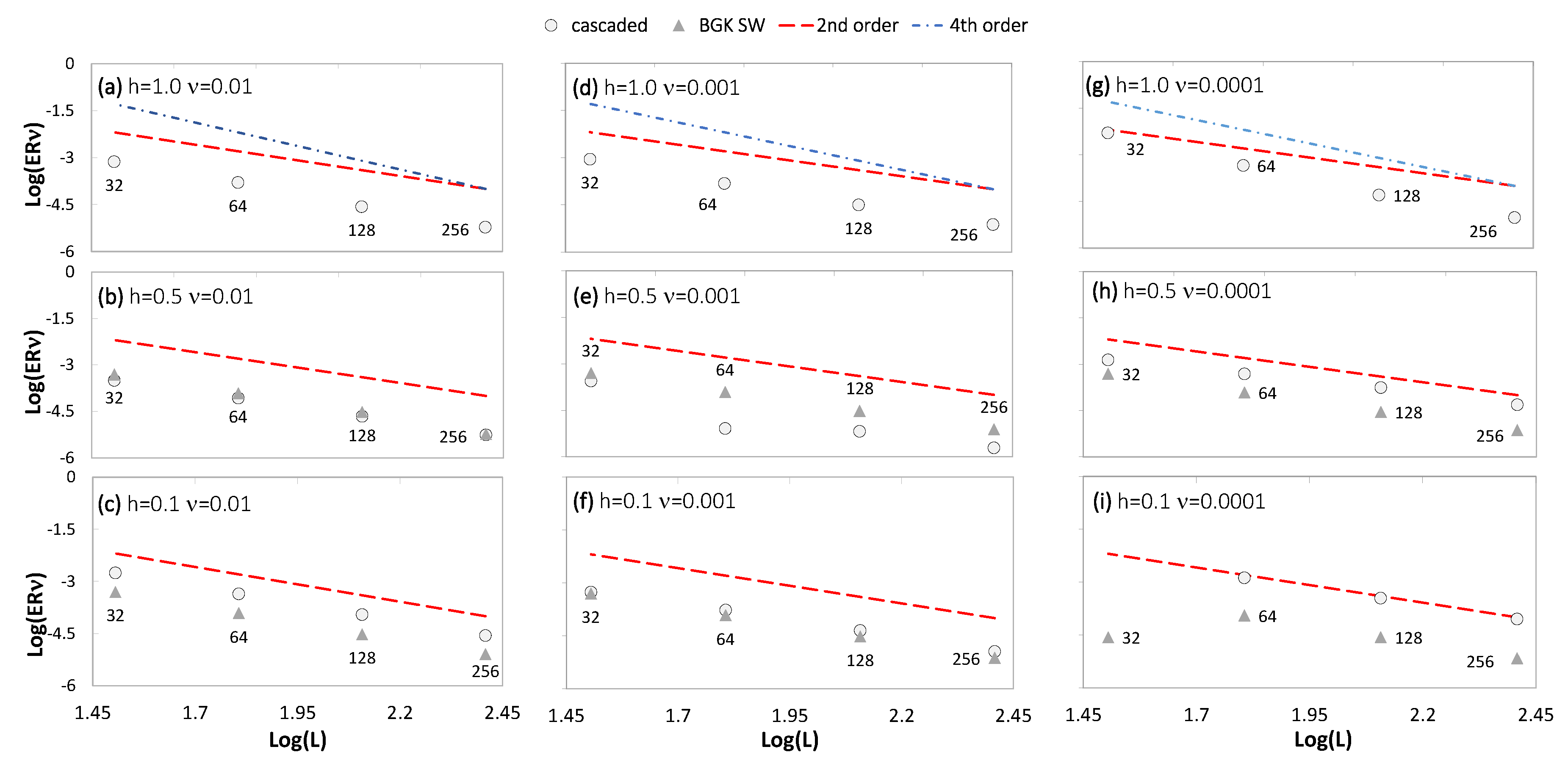
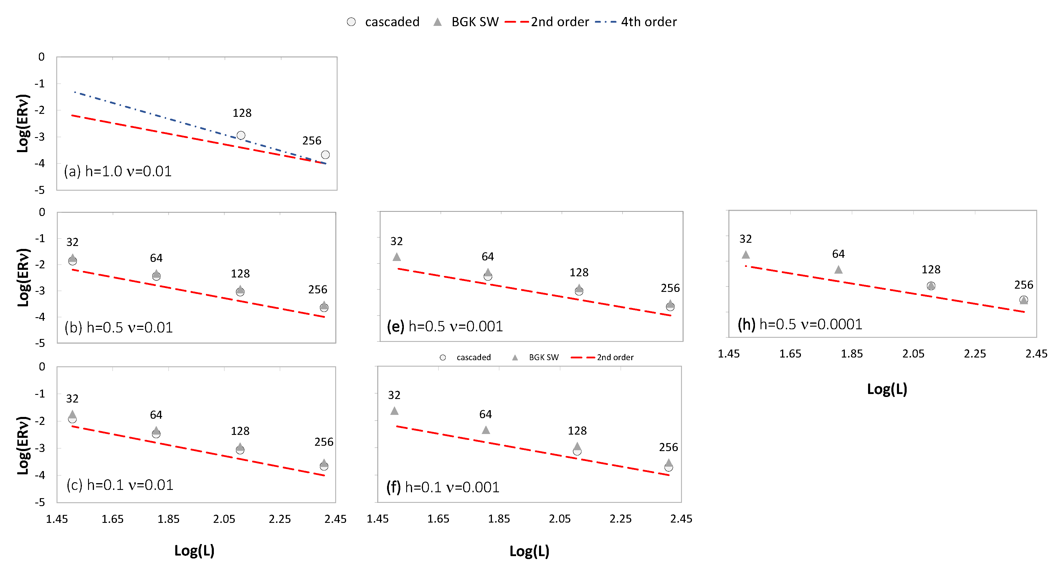
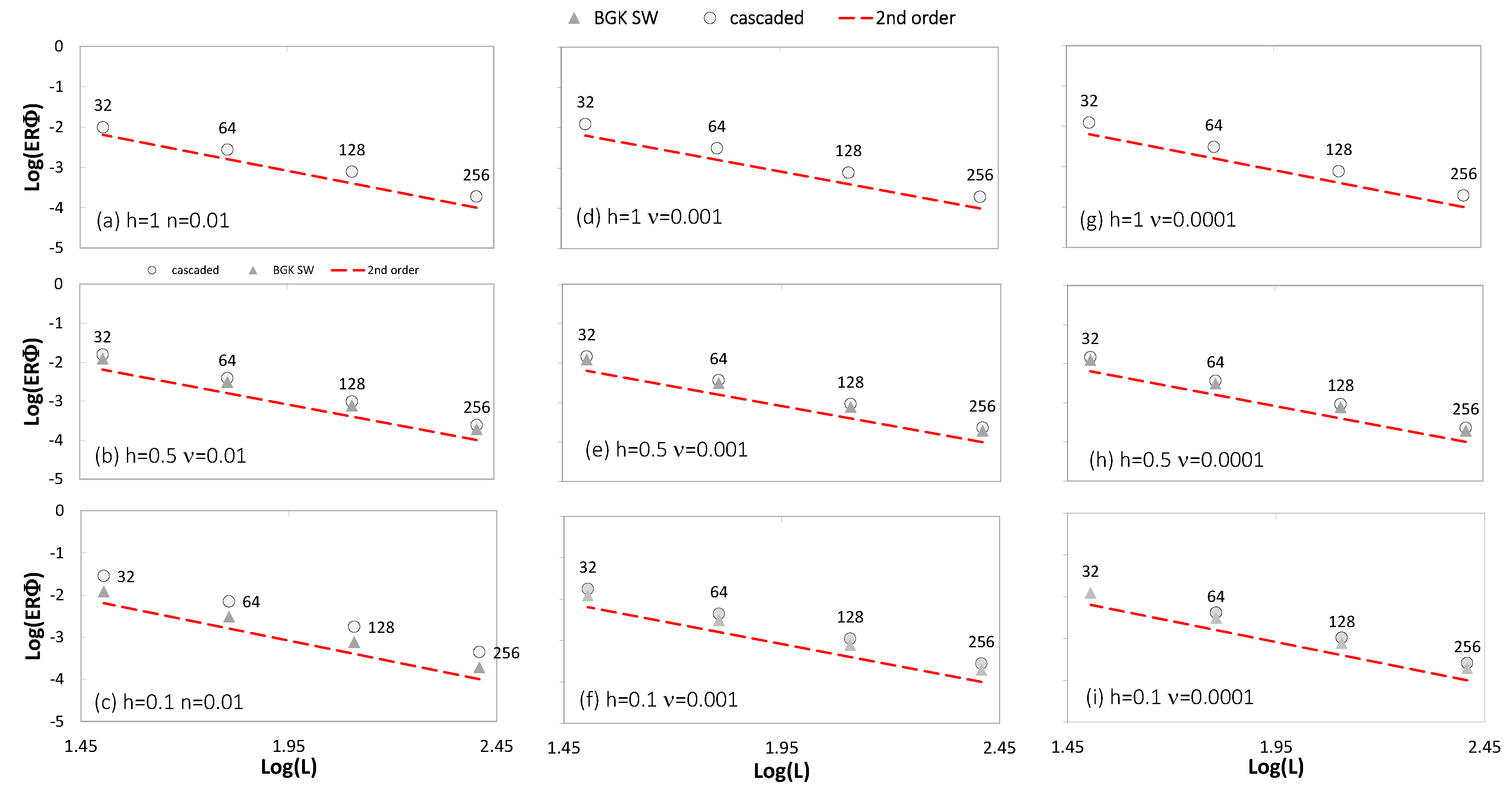
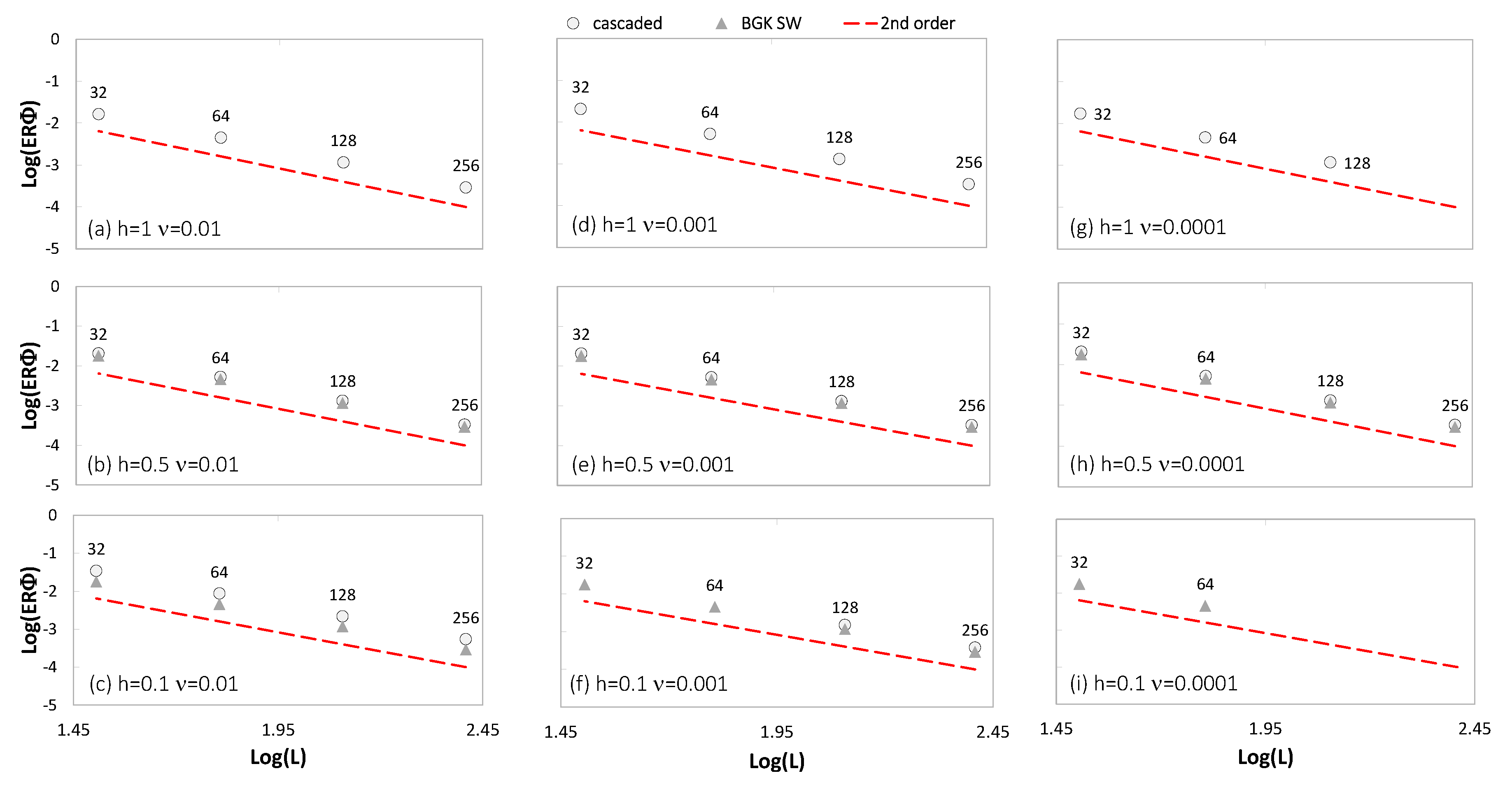
The results of the convergence study in [34], measuring the error in diffusive scaling, is summarized below. In the solution of the SWE, the CaLB and BGK models differ in the way of imposing an isotropic viscosity. The asymptotic behavior of the measured viscosity $\nu$ is determined by fitting the logarithm of the amplitude of a decaying wave to a linear function. The phase lag, measured when the wave should have come back to its original position, is an indicator of the models violation of Galilean invariance. The Taylor Green Vortex test case allows to compare the behavior of CaLB and BGK models for various values of viscosities ($\nu$) and water depths (h) and two different velocity configurations, namely, “slow set” and “fast set” (Appendix A, Figure A1, Figure A2, Figure A3 and Figure A4).

It is possible to observe that the two models, when stable, show a second-order convergence in viscosity error and in phase error. The h characterized by the most stable behavior is 0.5. Here, the simulations are stable for all the value of the viscosities taken into consideration. If the value of the depth moves towards lower or higher values, the stability properties change. The CaLB model is characterized by a wider stability range than the BGK model. In particular, it exhibits instability for h = 1.0 and low viscosities ($\nu$ = 0.01, $\nu$ = 0.001 and $\nu$ = 0.0001). It starts to become stable only for viscosities $\nu$ > 0.1. It is clarified that all the quantities are in lattice units.

3.2. Flow over a Bump

The first test case for the forcing schemes is the one-dimensional problem of a resting fluid in a channel. The numerical method is considered well balanced if the stationary solution on an uneven bed is perfectly reproduced [3]. The set-up of the simulation is the same as in [35]. The channel is 1 m long and the boundary conditions (BC) are periodic at the east and west boundaries. On the south/north boundaries the bounce-back BC is imposed. The parameters of the numerical simulation are $\Delta x$ = 0.01 m, $\Delta t$ = 0.026 s, and $\tau$ = 0.85. The bed topography equation is

$$z_b\left(x\right)=\left\{\begin{array}{c}0.25\left(cos\frac{\pi \left(x-0.5\right)}{0.1}+1\right)\left|x-0.5\right|\le 0.1\hfill \\ 0otherwise\hfill \end{array}\right.$$

(24)

Initially, the water is at rest ($\mathit{u}$ = 0) with the water surface (WS) level, $h+z_b$, equal to 1 m where h is the water depth. The exact solution for this case is a zero velocity and WS = $h+z_b$ = 1 m. The force term related to the bed topography is expressed by the Equation (15). The continuous form of the gravity force:

$$F_i=-gh\frac{\partial z_b}{\partial x_i}$$

(25)

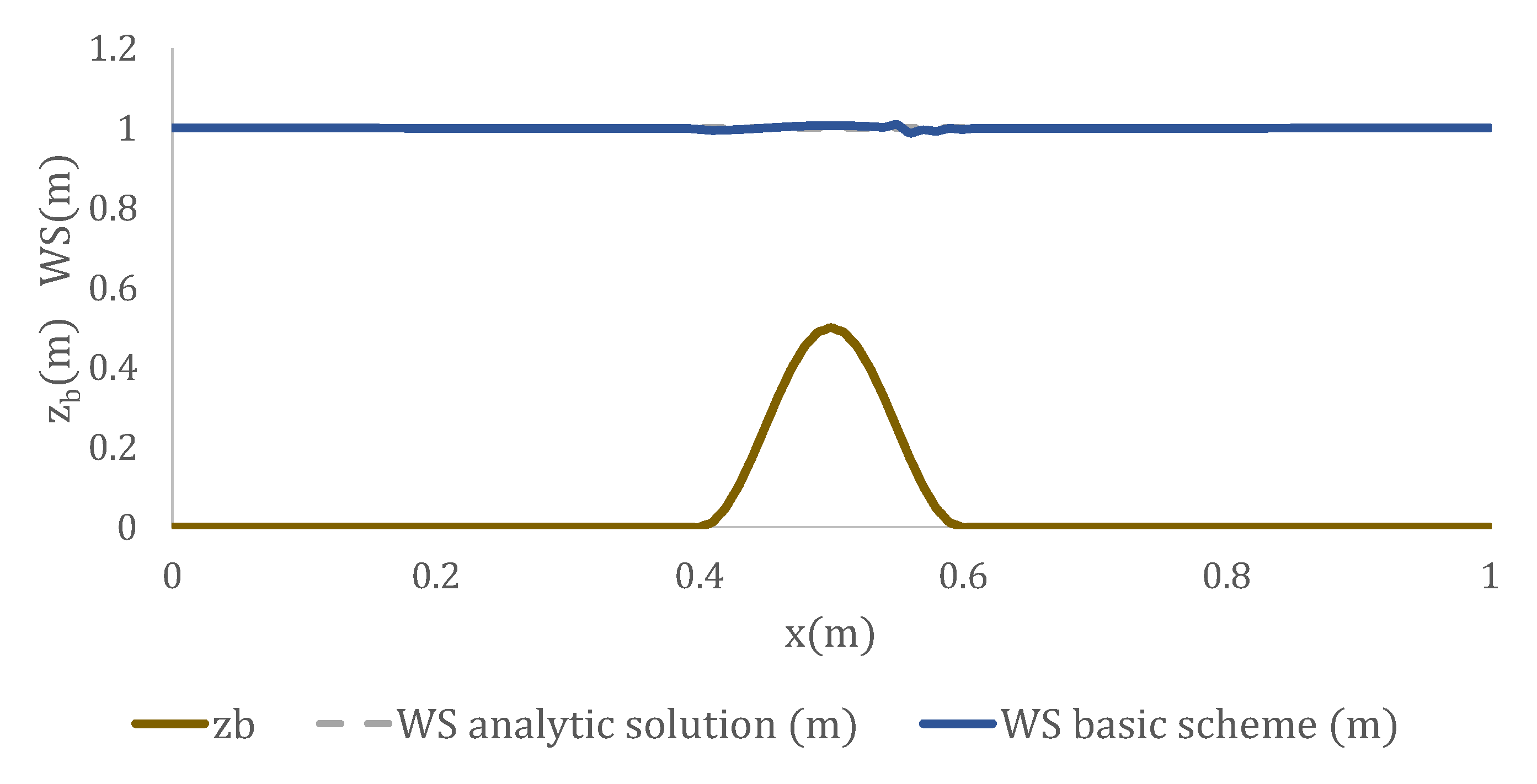
has been discretized using basic, second-order, and centred scheme. Figure 1 shows the WS in the CaLB model that uses the basic scheme to simulate the force. The steady state is reached after 5000 time steps. The WS shows an irregular trend over the bump and the simulation becomes unstable at 9000 time steps. The artificial velocity created along the x-axis increases, leading to the instability of the numerical simulation.

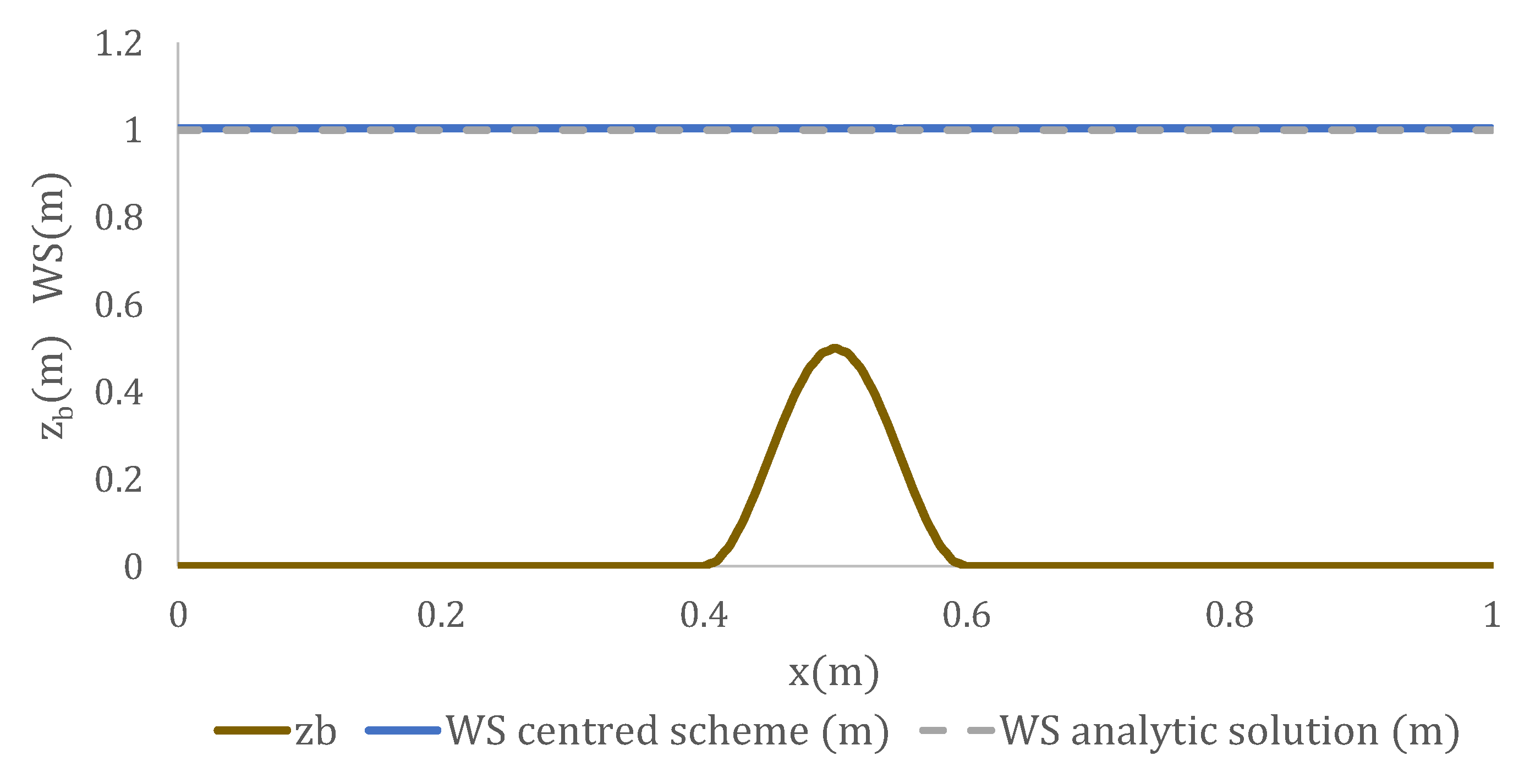
In Figure 2 the steady-state solution for the centred scheme of the force is shown. It is reached after 1000 time steps and corresponds to the analytical solution. In this scheme, the value of the velocity remains very low ($<={10}^{-3}$ m/s). Moreover, the simulation runs until 10,000 time steps and continues to be stable. In contrast, as it has been already shown in [3], the second-order scheme leads to a profile of the WS with a relative error as large as ~20%. Reaching steady state takes much longer for the second-order scheme than for the centred scheme (≅5000 time steps) and the spurious velocities are much higher (≅0.06 m/s). According to results obtained by Zhou for the BGK collision operator [3], it is found that only the centred scheme can produce accurate results in agreement with the analytical solution.

3.3. Poiseuille Flow with External Force

One of the known solutions for nonlinear kinetic equations is the steady plane Poiseuille flow in a channel of $2L$ width and with constant water depth [36]. For this case, the shallow water equations simplify to an ordinary differential equation of the flow velocity in the x direction u: $\nu \frac{{\partial }^{2}u}{{\partial y}^2}+F_x=0$, where $F_x$ is the source term in the x direction. If a no-slip boundary condition is applied at $y=\pm L$ (L is the lateral distance from the middle of the channel width), i.e., $u\left(y\right)=0$ when $y=\pm L$, the analytical solution is a parabola:

$$u\left(y\right)=\frac{F_x}{2\nu }\left(L^2-y^2\right)$$

(26)

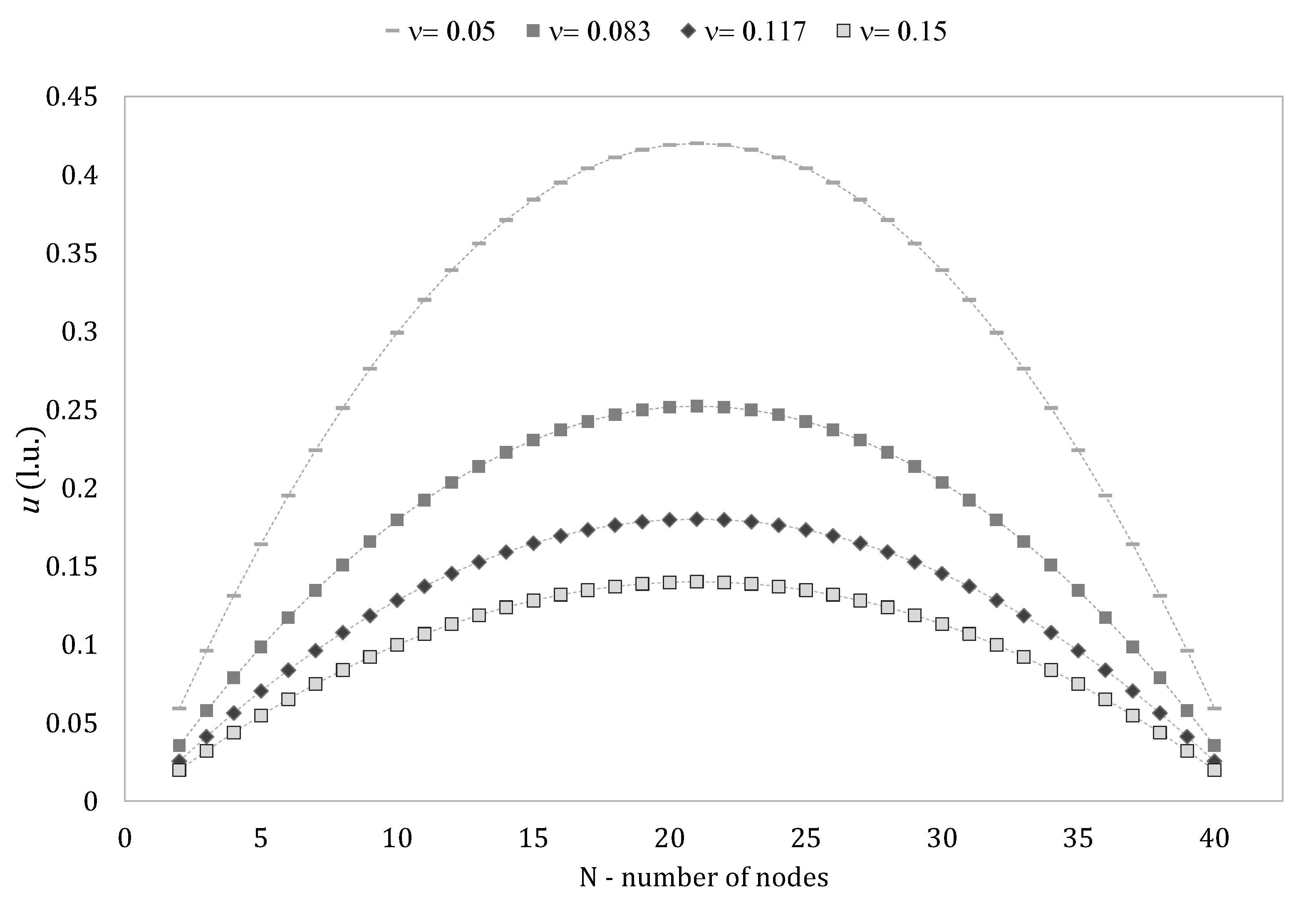
In this test case, the water depth is h = 1 m, the channel is 400 m long and 40 m wide; $\Delta x$ = 1 m and $\Delta t$ = 1 s. To test the decrease in accuracy with the viscosity, different relaxation times $\tau$ are considered: 0.95, 0.85, 0.75, and 0.65, which are correspondent, respectively, to the viscosities $\nu$ (Equation (6)): 0.15, 0.117, 0.083, and 0.05 in lattice units (l.u.). The value of $F_x$ is equal to 0.001 in lattice unit.

In Figure 3, the profile of the velocities of the numerical model perfectly corresponds to the analytical solution, for different viscosities. The $L_2$ norm (

Table 1. $L_2$ norm for different viscosities. $L_2=\frac{\sqrt{{\sum }_x^{}{∥u_n\left(x,t\right)-u_a\left(x,t\right)∥}^2}}{\sqrt{{\sum }_x^{}{∥u_n\left(x,t\right)∥}^2}}$ where $u_n$ and $u_a$ are, respectively, the numerical and the analytical value.

$\mathit{\tau }$	${\mathit{L}}_2$ Norm
0.95	0.00017
0.85	0.00020
0.75	0.00029
0.65	0.00052

) increases very slightly with the reduction of the viscosity. For the given set of parameters and resolution, it is $O\left({10}^{-4}\right)$. The $L_2$ norm is preferred here over the $L_{\infty }$ and $L_1$ norms. An advantage of this norm is that local errors cannot cancel each other and the error remains conditioned by any deviation from the analytical solution [37].

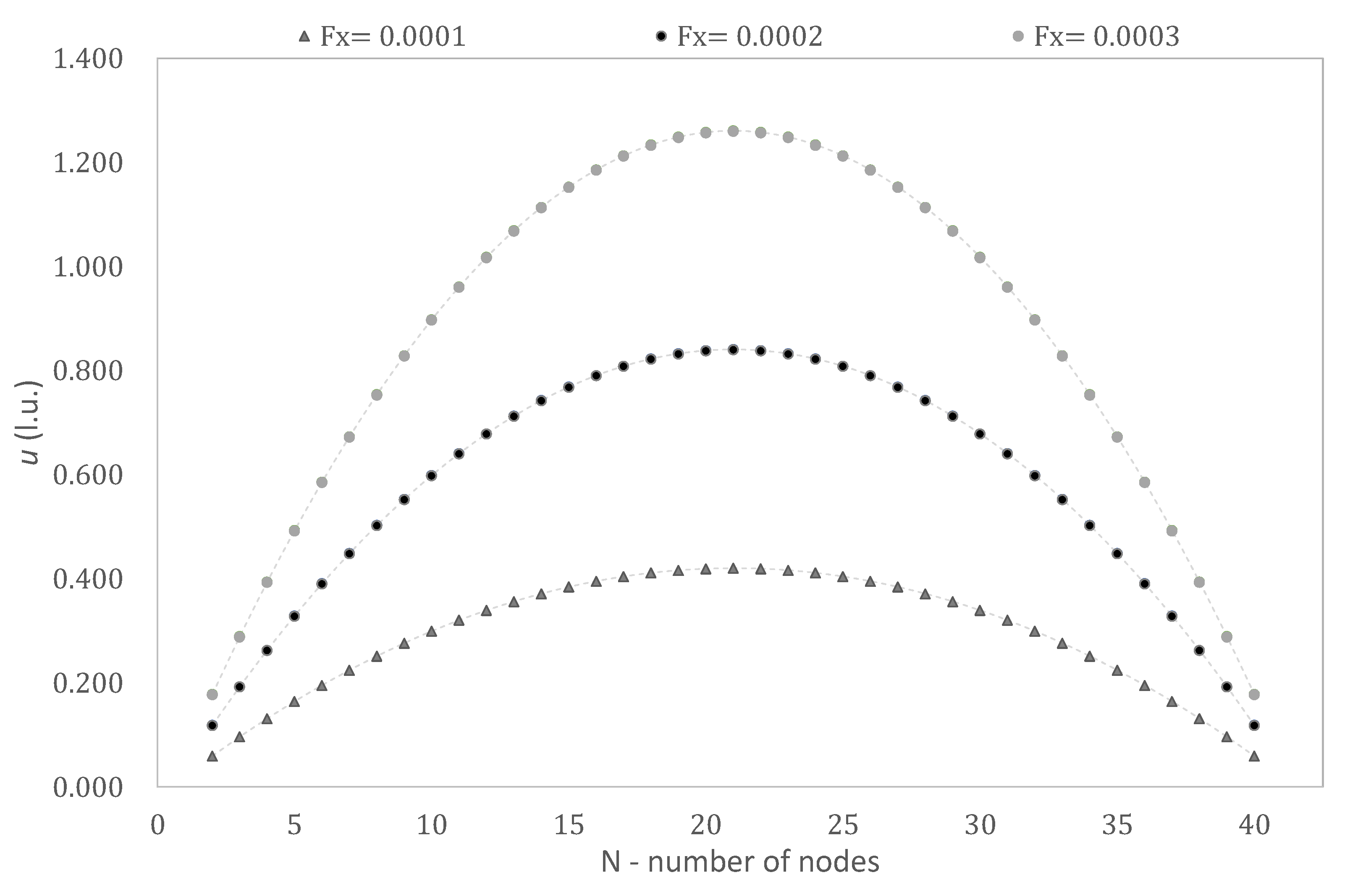
In Figure 4, it can be observed that the profile of the velocities of the numerical model, for increasing values of the force, perfectly corresponds to the analytical solution. The reason for the slight increase of the $L_2$ norm with increasing forcing (

Table 2. $L_2$ norm for different value of the force $F_x$—Forces expressed in l.u.

Force ${\mathit{F}}_{\mathit{x}}$	${\mathit{L}}_2$ Norm
0.0001	0.00053
0.0002	0.00058
0.0003	0.00070

) was not investigated in detail, but it is most probably linked to the higher velocity associated with larger forces. Equation (15) distributes the force over the lattice directions with weights taken for a resting fluid. Determining the weights dynamically, according to the local velocity, could improve the results but might also introduce errors as the velocity at the lattice links would have to be interpolated from the lattice nodes.

3.4. Flow Over a Two-Dimensional Bump

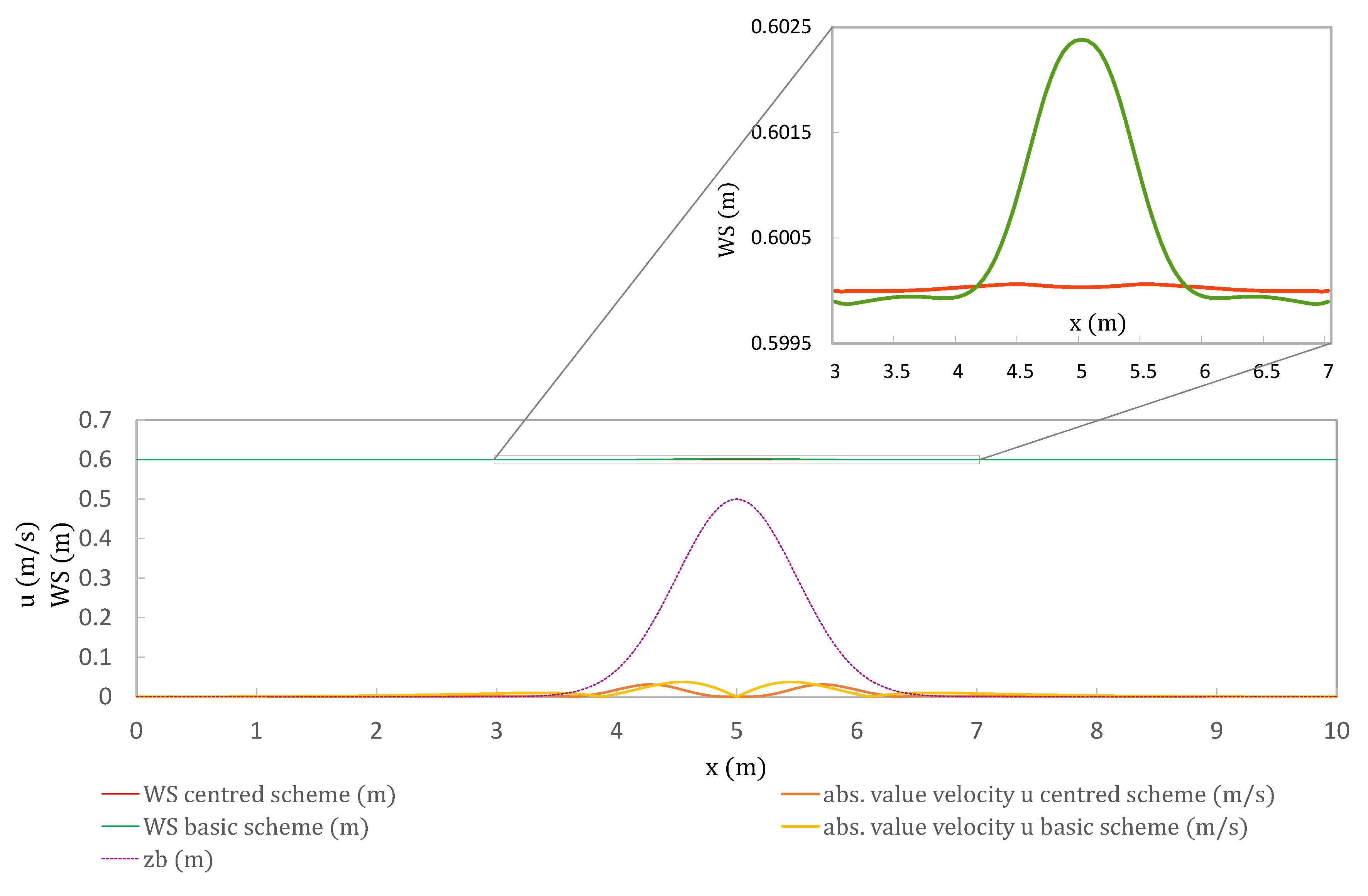
The simple two-dimensional case of resting water over a variable bottom is investigated next. The domain is a 10 m long and 10 m wide basin and the initial water level is 0.6 m. The equation that describes the bed is

$$z_b\left(x,y\right)=\left\{\begin{array}{c}0.5e^{-2\left[{(x-5)}^2+{(y-5)}^2\right]}{(x-5)}^2+{(y-5)}^2\le 4\hfill \\ 0otherwise\hfill \end{array}\right.$$

where $z_b$, x, and y are expressed in meters. In the numerical model we considered a relaxation time $\tau$ = 0.505, a spatial and temporal resolution of $\Delta x$ = 0.05 m and $\Delta t$ = 0.01 s, respectively. Periodic conditions are applied at all the boundaries. The steady state is reached after 15 s for both schemes. It is observed that, in this test, the basic scheme is stable, but leads to a profile of the water surface not in agreement with the analytical solution showing a flat water surface. After 15 s, the basic model shows spurious velocities with values higher than the centred model by ~17% (Figure 5). To test the accuracy of the CaLB model with a centred-scheme force the error ($L_2$) for different space resolutions was calculated and is shown in the following

Table 3. WS $L_2$ norms—correspondence of numerical results with analytical solution.

$\Delta \mathit{x}$ (m)	${\mathit{L}}_2$
0.05	0.0000691
0.025	0.00000743
0.0125	0.00000138

: the error norm $L_2$ decreases with the space resolution, with a trend slightly higher than second order.

4. Conclusions

The present work examines a lattice Boltzmann approach based on the use of a non conventional MRT collision operator, the cascaded CO, co-moving with the fluid. The model maintains good accuracy and stability even after the introduction of the treatment of the external forces. Model validation is performed through comparison with literature case studies (one-dimensional and two-dimensional bump, Poiseuille flow between two plan plates), highlighting a good correspondence between simulated and literature data. Specifically, different implementation schemes of the force are considered in 1D bump test case, and the best results are achieved using the centred scheme. Our results (water depth and velocity value) are in accordance with the ones in literature using the BGK model. The Poiseuille test case allows to demonstrate the good behavior of the model for decreasing of the viscosity and increasing of the force value. Finally, the 2D bump test case puts in evidence the positive results of the CaLB that uses the centred scheme to model the force. Considering a low viscosity value, close to the water viscosity, the CaLB model remains stable with a second-order accuracy. The presentation of the convergence study of the cascaded model in comparison with the standard BGK model exhibits the advantages of the novel model, in particular, from the stability point of view.

The first results of the CaLB show that the proposed methodology represents a promising tool for simulation of shallow water flows.

References

- Venturi, S.; Di Francesco, S.; Geier, M.; Manciola, P. A new collision operator for lattice Boltzmann shallow water model: A convergence and stability study. Adv. Water Resour. 2020, 135, 103474. [Google Scholar] [CrossRef]
- Toro, E. Shock-Capturing Methods for Free-Surface Shallow Flows; John Wiley: New York, NY, USA, 2001. [Google Scholar]
- Zhou, J.G. Lattice Boltzmann Methods for Shallow Water Flows; Springer: Berlin, Germany, 2004. [Google Scholar]
- Prestininzi, P.; Sciortino, G.; Rocca, M.L. On the effect of the intrinsic viscosity in a two-layer shallow water lattice Boltzmann model of axisymmetric density currents. J. Hydraul. Res. 2013, 51, 668–680. [Google Scholar] [CrossRef]
- Salmon, R. The lattice Boltzmann method as a basis for ocean circulation modeling. J. Mar. Res. 1999, 57, 503–535. [Google Scholar] [CrossRef]
- Meselhe, E.A.; Sotiropoulos, F.; Holly, F.M. Numerical Simulation of Transcritical Flow in Open Channels. J. Hydraul. Eng. 1997, 123, 774–783. [Google Scholar] [CrossRef]
- Valiani, A.; Caleffi, V.; Zanni, A. Case Study: Malpasset Dam-Break Simulation using a Two-Dimensional Finite Volume Method. J. Hydraul. Eng. 2002, 128, 460–472. [Google Scholar] [CrossRef]
- Tubbs, K.R.; Tsai, F.T.C. MRT-Lattice Boltzmann Model for Multilayer Shallow Water Flow. Water 2019, 11, 1623. [Google Scholar] [CrossRef] [Green Version]
- Stansby, P.K.; Zhou, J.G. Shallow-water flow solver with non-hydrostatic pressure: 2D vertical plane problems. Int. J. Numer. Methods Fluids 1998, 28, 541–563. [Google Scholar] [CrossRef]
- Prestininzi, P.; Lombardi, V.; La Rocca, M. Curved boundaries in multi-layer Shallow Water Lattice Boltzmann Methods: Bounce back versus immersed boundary. J. Comput. Sci. 2016, 16, 16–28. [Google Scholar] [CrossRef]
- Toro, E. Riemann problems and the WAF method for solving two-dimensional shallow water equations. Phil. Trans. R. Soc. Lond. A 1992, 338, 43–68. [Google Scholar]
- Vazquez, M.E. Improved Treatment of Source Terms in Upwind Schemes for the Shallow Water Equations in Channels with Irregular Geometry. J. Comput. Phys. 1999, 148, 497–526. [Google Scholar] [CrossRef]
- Bermudez, A.; Vazquez, M.E. Upwind methods for hyperbolic conservation laws with source terms. Comput. Fluids 1994, 23, 1049–1071. [Google Scholar] [CrossRef]
- Benkhaldoun, F.; Elmahi, I.; Seaı, M. Well-balanced finite volume schemes for pollutant transport by shallow water equations on unstructured meshes. J. Comput. Phys. 2007, 226, 180–203. [Google Scholar] [CrossRef] [Green Version]
- Vukovic, S.; Sopta, L. ENO and WENO schemes with the exact conservation property for one-dimensional shallow water equations. J. Comput. Phys. 2002, 179, 593–621. [Google Scholar] [CrossRef]
- Di Francesco, S.; Biscarini C, M.P. Modelli mesoscopici per le correnti a superficie libera. In Atti del XXXV Convegno Nazionale di Idraulica e Costruzioni Idrauliche; DICAM Università di Bologna: Bologna, Italy, 2016. [Google Scholar]
- Banari, A.; Janßen, C.; Grilli, S.T.; Krafczyk, M. Efficient GPGPU implementation of a lattice Boltzmann model for multiphase flows with high density ratios. Comput. Fluids 2014, 93, 1–17. [Google Scholar] [CrossRef]
- Luo, L.S. Lattice-Gas Automata and Lattice Boltzmann Equations for Two-Dimensional Hydrodynamics. Ph.D. Thesis, Georgia Institute of Technology, Atlanta, GA, USA, 1993. [Google Scholar]
- Shan, X.; Chen, H. Simulation of non ideal gases and gas-liquid phase transitions by the lattice Boltzmann Equation. Phys. Rev. E 1994, 49, 697. [Google Scholar] [CrossRef] [PubMed] [Green Version]
- Buick, J.; Greated, C. Gravity in a lattice Boltzmann model. Phys. Rev. E 2000, 61, 5307. [Google Scholar] [CrossRef] [Green Version]
- Falcucci, G.; Ubertini, S.; Bella, G.; De Maio, A.; Palpacelli, S. Lattice Boltzmann modeling of diesel spray formation and break-up. SAE Int. J. Fuels Lubr. 2010, 3, 582–593. [Google Scholar] [CrossRef]
- Di Francesco, S.; Zarghami, A.; Biscarini, C.; Manciola, P. Wall roughness effect in the lattice Boltzmann method. AIP Conf. Proc. 2013, 1558, 1677–1680. [Google Scholar]
- Yang, X.; Mehmani, Y.; Perkins, W.; Pasquali, A.; Schönherr, M.; Kim, K.; Perego, M.; Parks, M.; Trask, N.; Balhoff, M.; et al. Intercomparison of 3D pore-scale flow and solute transport simulation methods. Adv. Water Resour. 2016, 95, 176–189. [Google Scholar] [CrossRef] [Green Version]
- Zarghami, A.; Francesco, S.D.; Biscarini, C. Porous substrate effects on thermal flows through a REV-scale finite volume lattice Boltzmann model. Int. J. Mod. Phys. C 2014, 25, 1350086. [Google Scholar] [CrossRef]
- Di Francesco, S.; Biscarini, C.; Manciola, P. Characterization of a flood event through a sediment analysis: The Tescio River case study. Water 2016, 8, 308. [Google Scholar] [CrossRef] [Green Version]
- Biscarini, C.; Di Francesco, S.; Ridolfi, E.; Manciola, P. On the Simulation of Floods in a Narrow Bending Valley: The Malpasset Dam Break Case Study. Water 2016, 8, 545. [Google Scholar] [CrossRef] [Green Version]
- Dellar, P.J. Nonhydrodynamic modes and a priori construction of shallow water lattice Boltzmann equations. Phys. Rev. E Stat. Nonlinear Soft Matter Phys. 2002, 65, 036309. [Google Scholar] [CrossRef] [PubMed] [Green Version]
- Geier, M.; Pasquali, A. Fourth order Galilean invariance for the lattice Boltzmann method. Comput. Fluids 2018, 166, 139–151. [Google Scholar] [CrossRef]
- Qian, Y.H.; D’Humières, D.; Lallemand, P. Lattice BGK Models for Navier–Stokes Equation. EPL Europhys. Lett. 1992, 17, 479. [Google Scholar] [CrossRef]
- D’Humières, D. Generalized lattice-Boltzmann equations. Prog. Astronaut. Aeronaut. 1994, 159, 450. [Google Scholar]
- Geier, M.; Schönherr, M.; Pasquali, A.; Krafczyk, M. The cumulant lattice Boltzmann equation in three dimensions: Theory and validation. Comput. Math. Appl. 2015, 70, 507–547. [Google Scholar] [CrossRef] [Green Version]
- Geier, M. Ab Initio Derivation of the Cascaded Lattice Boltzmann Automaton. Ph.D. Thesis, University of Freiburg, Breisgau, Germany, 2006. [Google Scholar]
- Premnath, K.N.; Banerjee, S. Incorporating forcing terms in cascaded lattice Boltzmann approach by method of central moments. Phys. Rev. E 2009, 80, 036702. [Google Scholar] [CrossRef] [Green Version]
- Venturi, S. Lattice Boltzmann Shallow Water Equations for Large Scale Hydraulic Analysis. Ph.D. Thesis, University of Florence, Pisa, Perugia and Technische Universität Braunschweig, Braunschweig, Germany, 2018. [Google Scholar]
- LeVeque, R.J. Balancing Source Terms and Flux Gradients in High-Resolution Godunov Methods: The Quasi-Steady Wave-Propagation Algorithm. J. Comput. Phys. 1998, 146, 346–365. [Google Scholar] [CrossRef] [Green Version]
- Liu, H. Lattice Boltzmann Simulations for Complex Shallow Water Flows. Ph.D. Thesis, University of Florence, Liverpool, UK, 2009. [Google Scholar]
- Timm, K.; Kusumaatmaja, H.; Kuzmin, A.; Shardt, O.; Silva, G.; Viggen, E. The Lattice Boltzmann Method, Principles and Practice; Springer: Cham, Switzerland, 2016; p. 694. [Google Scholar]
Figure 1.
Basic-scheme: WS after 5000 time steps.
Figure 2.
Centred-scheme: WS after 1000 time steps.
Figure 3.
Velocity profiles for different relaxation times = 0.95, 0.85, 0.75, 0.65.
Figure 4.
Velocity profiles for different values of the x component of the force —transversal section of the channel.
Figure 5.
Comparison of basic scheme and centred scheme. bottom level (m), WS (m), and spurious velocities (m/s).