Study on the Characteristic Point Location of Depth Average Velocity in Smooth Open Channels: Applied to Channels with Flat or Concave Boundaries

Abstract

Based on the flow partition theory, we derive a mathematical expression by using the log-law for the characteristic point location (CPL) of depth average velocity in channels with flat or concave boundaries. It can manifest the position of the characteristic points in the vertical direction relative to the channel side wall or bed. Taking rectangular and semi-circular channels as research objects, we put forward a method to calculate the discharge of channels with CPL. Additionally, we carried out some experiments on rectangular and semi-circular channel sections. CPL’s analytic expression is validated against experimental results through comparison of velocity and discharge. The proposed formulation of characteristic point location could be extensively employed in flow measurements of flat and concave boundary channels, which has practical application value in simplifying the flow measurement steps of open channels.

1. Introduction

The contradiction between the serious shortage of agricultural water resources and unreasonable utilization has been restricting the development of agricultural economy [1]. Precision agriculture provides the potential to enhance irrigation efficiency through specific methods of flow measurement in channels.

Flow measurement methods through weir-gate structures [2] and velocity–area methods are widely used in flow measurement. The principle of a sluice gate or weir is based on the concept of critical flow, making it possible to measure only the depth and calculate the flow rate, thus simplifying the continuous monitoring of flow rate [3]. However, critical flow in open channels can be formed through two general methods: raising the bottom of the channel or contracting the cross-sectional area of the flow [3,4]. Neither of these two methods is easy to implement. Impurities on the sluice gate or weir accumulate easily and need to be cleaned regularly, which is difficult to achieve during actual production. Apart from measuring with weir-gate structures, the velocity–area method for calculating discharge in an open channel is considered to be particularly reliable. However, a large number of measurements results in an associated time cost of measurement. Numerous researchers have proposed different forms of the velocity distribution law in order to predict flow discharge accurately.

The study of velocity distribution is critical to the calculation of the discharge. Relevant research can be traced back to the 1930s. In 1938, Keulegen [5] first proposed that the log-law could be used to describe the time-averaged velocity distribution of fully developed open channel uniform turbulence:

$$\frac{u}{u_{\ast }}=\frac{1}{\kappa }\ln \frac{u_{\ast }\times y}{\nu }+\omega$$

(1)

where u is the velocity in the channel, $u_{\ast }$ is frictional velocity, $\nu$ is the coefficient of kinematic viscosity, $\kappa$ is the von Kármán constant, and $\omega$ is constant.

Nikuradse made an artificial sand rough pipe using pasting sand with a uniform particle size on the wall of a pipe [6,7]. The analysis of the experimental data of the smooth sand tube showed that the values of parameters $\kappa$ and $\omega$ in log-law are 0.4 and 5.5. Different researchers have given different values of the von Kármán constant $\kappa$ and constant $\omega$ according to their experimental data [8,9,10]. This paper uses the parameter values given by Nikuradse for further derivation.

Under the guide of velocity distribution, researchers have used different methods to measure velocity. Chiu [11,12,13] developed the entropy model, correlating the mean flow velocity to the maximum value using the linear relationship Um = φ(M)U_max, which depends on the entropic parameter M. Maghrebi [14] used the similarity between the magnetic field of a current wire and the isovel contours in a channel cross-section to derive the isovel patterns. Then, one can easily obtain the discharge using a single point on the isovel patterns of velocity measurement. However, the measured points are only selected from the upper half of the water depth and away from the boundaries, which would be much closer to the measured discharge. Bretheim et al. [15] used the restricted nonlinear (RNL) model to simulate wall turbulence and obtained the real mean velocity distribution in the channel at a low Reynolds number. Hong et al. [16] employed a systematic measuring technology combining ground-penetrating radar and surface velocity radar and established the rating curves representing the relation of water surface velocity to the channel cross-sectional mean velocity and flow area. Then, stream discharge was deduced from the resulting mean velocity and flow area. Moramarco et al. [17] proposed a new method for estimating discharge from surface velocity monitoring (u_surf). Based on entropy theory and sampling u_surf, it can identify the two-dimensional velocity distribution in the cross-sectional flow area. This method is more accurate for rivers with a lower aspect ratio where secondary currents are expected. Johnson and Cowen [18,19] predicted the mean streamwise velocity and the depth-averaged velocity by permitting remote determination of the velocity power-law exponent. Then, the volumetric discharge from surface measurements of currents can be determined. Khuntia et al. [20] presented a new methodology to predict the depth-averaged velocity. They used multi-variable regression analysis to develop five models to predict the point velocities in terms of non-dimensional geometric and flow parameters at any desired location. Through these attempts, researchers have discussed new thoughts of quantifying channel discharge. But few people determine the average velocity of a channel by looking for the location of characteristic points.

Overall, this study investigates a new concept of characteristic point location aimed at estimating the discharge in open channels, which is based on flow partitioning theory and the log-law. This method is applied to flat channels (e.g., a rectangular channel) and concave channels (e.g., a semi-circle channel). The derived theoretical expression of characteristic point location is also verified by the experimental data. We expect that the method for flow measurement conveniently proposed by this paper could be used widely for different varieties of irrigation channels.

2. Methodology

This paper assumes that characteristic points exist on the channel cross-section whose velocities could be called characteristic velocities. We can measure these points to get the precise measurements of velocity and discharge. The positions of these points are called characteristic point locations of depth average velocity (CPL).

2.1. CPL in Rectangular Channels

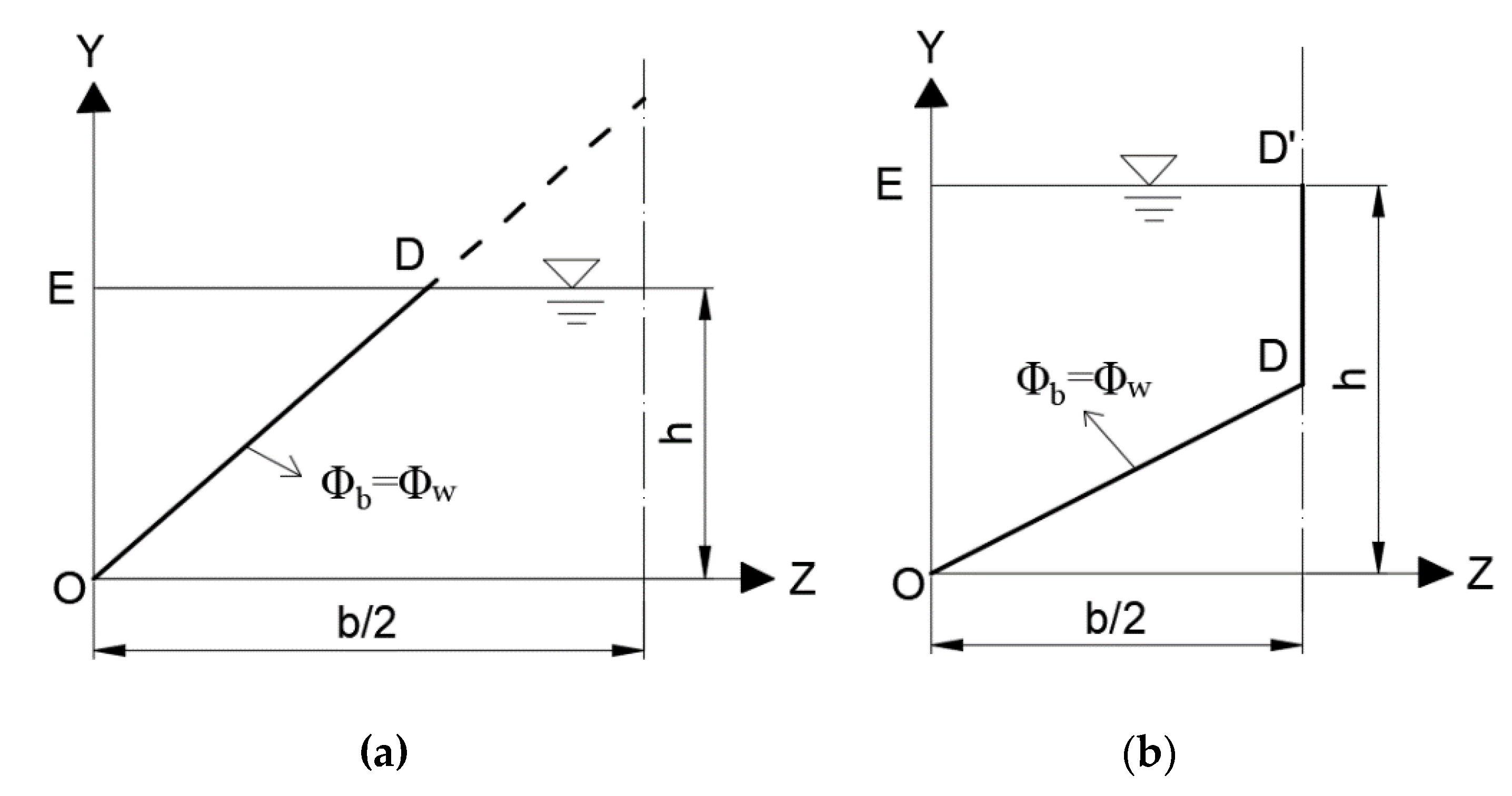
2.1.1. Existing Form of the Division Line in Rectangular Channels

Consider the case of steady, uniform flow in a smooth rectangular channel with an aspect ratio of b/h, where h = water depth and b = channel width. Due to existence of a secondary current, the division line is actually a zero Reynolds shear stress line in the flow area, and also a line without energy cross-transfer [21]. Yang et al. [22] have proven the physical existence of division lines by using experimental data recorded at the Hydraulics Laboratory, University of Wollongong, as well as the experimental data recorded previously by Melling and Whitelaw [23] and that of Tracy [24].

Einstein [25] proposed that the flow cross-sectional area can be divided into three sub-sections that correspond to the side wall and channel bed. However, he did not propose any method of determining the exact location of the division line. Chien and Wang [26] performed an in-depth study of Einstein’s idea. They gave the total overall boundary shear stress, ${\tau }_0$, as:

$${\tau }_0=\rho gR{S}_e$$

(2)

where $\rho$ = fluid density; g = gravitational acceleration; R = hydraulic radius; and S_e = energy slope.

Then, they divided ${\tau }_0$ into two parts corresponding to the bed, $\overline{{\tau }_b}$, and side wall, $\overline{{\tau }_w}$. They also defined two hydraulic radii, one for the wall $R_w$, and one for the bed $R_b$. Thus:

$$\overline{{\tau }_w}=\rho g{R}_w{S}_e=\rho g{S}_e{A}_w/h$$

(3)

$$\overline{{\tau }_b}=\rho g{R}_b{S}_e=\rho g{S}_e{A}_b/b$$

(4)

where $\overline{{\tau }_b}$ = mean bed shear stress;$\overline{{\tau }_w}$ = mean wall shear stress; A_b = flow area corresponding to channel bed; A_w = flow area corresponding to channel side wall; R_w = hydraulic radius corresponding to side wall; and R_b = hydraulic radius corresponding to bed.

According to Yang [27], the mechanical energy contained in any flow will be transmitted to the boundary nearest to the “relative distance” and dissipated. The dimensionless relative distance Φ is defined as the ratio of geometrical length between a point in the flow field and the characteristic boundary length, representing the energy dissipation capacity of the boundary (for a smooth boundary channel, this would be the viscous layer thickness D_s).

The side wall and bed will each have their own fair share of surplus energy transferred from the main flow depending on the minimum relative distance Φ. Accordingly, for any unit volume in the flow field, there are two possible ways to transfer the surplus energy: either toward the bed (${\mathsf{\Phi }}_b$) or toward the side wall (${\mathsf{\Phi }}_w$). If ${\mathsf{\Phi }}_w\le {\mathsf{\Phi }}_b$, the energy will be transferred toward the side wall. Conversely, if ${\mathsf{\Phi }}_w\ge {\mathsf{\Phi }}_b$, then the energy will be transported to the bed. It follows that the condition where ${\mathsf{\Phi }}_w={\mathsf{\Phi }}_b$ will define a division line by which the flow region near the corner is divided into two sub-flow sections.

Therefore, the division line (${\mathsf{\Phi }}_w={\mathsf{\Phi }}_b$) in Figure 1a can be expressed as:

$$\frac{z}{D_{sw}}=\frac{y}{D_{sb}}$$

(5)

where z and y denote the horizontal and vertical axes in the Cartesian coordinates system, respectively; y = vertical direction normal to bed; z = transverse flow direction;$D_{sw}$ = characteristic length for smooth side wall; and $D_{sb}$ = characteristic length for smooth channel bed.

Substituting $D_{sw}=C_s\nu /\overline{u_{\ast w}}$ and $D_{sb}=C_s\nu /\overline{u_{\ast b}}$ into Equation (5) gives:

$$z=ky; k=\frac{\overline{u_{\ast b}}}{\overline{u_{\ast w}}}.$$

(6)

where $C_s$ = constant; $\overline{u_{\ast w}}$ = mean side wall shear velocity; and $\overline{u_{\ast b}}$ = mean bed shear velocity. The geometric significance of k in Figure 1a is the reciprocal of the slope of the line OD. Point D is the intersection of the division line and the water surface line.

Then, it can be obtained that:

$$R_w=\frac{A_w}{h}=\frac{\frac{1}{2}k{h}^2}{h}$$

(7)

$$R_b=\frac{A_b}{b}=\frac{bh-k{h}^2}{b}$$

(8)

Using Equations (3)–(8), k can be evaluated, yielding:

$$\frac{\overline{{\tau }_b}}{\overline{{\tau }_w}}=\frac{\rho {\overline{u_{\ast b}}}^2}{\rho {\overline{u_{\ast w}}}^2}=k^2=\frac{1-\frac{kh}{b}}{\frac{k}{2}}$$

(9)

Or:

$$k^3+(2h/b)k-2=0;\raisebox{1ex}{$b$}\!\left/ \!\raisebox{-1ex}{$h$}\right.\ge \alpha$$

(10)

Using a similar method, Yang and Lim [27] also gave the evaluation of k₁ in Figure 1b:

$$k_1{}^3+(b/2h)k_1-2=0;\raisebox{1ex}{$b$}\!\left/ \!\raisebox{-1ex}{$h$}\right.\le \alpha$$

(11)

where k₁ represents the slope of the division line OD in Figure 1b.

Highly inspired by the derivation of Yang and Lim [27], we also take the two cases of Figure 1 to analyze. It has been proven that the critical aspect ratio α is equal to 2 in smooth rectangular channels by Yang and Lim [27]. As the rectangle is axisymmetric, we take the vertical line of the channel section as the axis and only analyze half of it.

(a)

Determination of the location of division line in wide–shallow channel (b/h ≥ 2)

The division line can be determined by Equation (10) when b/h ≥ 2 (Figure 1a). Since $2h/b$ is a constant, solving Equation (10) will give the value of k.

Referring to the value of k, a comparison relationship between $1/k$ and $2h/b$ is as follows:

$$\frac{1}{k}-\frac{2h}{b}\ge 0$$

(12)

It can be shown from Inequality (13), so

$$\frac{1}{k}\ge \frac{2h}{b};\frac{2h}{b}\le 1$$

(13)

That is to say, when b/h ≥ 2, the slope of the division line is always greater than 2h/b. The intersection point of the division lines is on or above the water surface line.

(b)

Determination of the location of division line in narrow–deep channel (b/h ≤ 2)

The division line can be determined by Equation (11) when b/h ≤ 2 (Figure 1b). Since $b/2h$ is a constant, the value of k₁ can be obtained by solving Equation (11).

Referring to the value of k₁, a comparison relationship between k₁ and $2h/b$ is as follows:

$$k_1-\frac{2h}{b}\ge 0$$

(14)

It can be shown from Inequality (15), so

$$k_1\ge \frac{2h}{b};\frac{b}{2h}\le 1$$

(15)

That is to say, when b/h ≤ 2, the slope of the division line is always greater than 2h/b. The intersection point of the division lines is on or above the water surface line, the same as b/h ≥ 2.

By combining cases (a) and (b), we know that Figure 1b will not occur. Whether in a wide–shallow or in a narrow–deep channel, the existing form of the division line is always shown as Figure 1a.

2.1.2. CPL of Lines in Rectangular Channel

As shown in Figure 2, taking the left half cross-section of the channel as an example, the dividing line divides the cross-section of the channel into regions I (ABCD), II (OAD) and III (ODE).

In region I, the discharge of the shadow rectangle area can be expressed using Equation (16):

$$dQ=udA=udydz$$

(16)

where dQ is the discharge of the shadow rectangle area; dA is the area of shadow rectangle; and u is the longitudinal velocity of any point in the area.

By integrating y, the discharge Q can be obtained as follows:

$$Q=dz{\displaystyle {\int }_0^{h_I}udy}$$

(17)

As the rectangular area can be expressed as $A=h_{I}dz$, the average velocity of this flow area can be obtained as:

$$\overline{u}=\frac{Q}{A}=\frac{dz{\displaystyle {\int }_0^{h_I}udy}}{h_{I}dz}=\frac{{\displaystyle {\int }_0^{h_I}udy}}{h_I}$$

(18)

According to the log-law of vertical velocity in channel section:

$$\frac{u}{u_{\ast }}=2.5\ln \left(\frac{u_{\ast }y}{\nu }\right)+5.5$$

(19)

Substituting Equation (19) to (18) gives:

$$\overline{u}=2.5u_{\ast }\ln \frac{u_{\ast }\cdot h_I}{\nu }+3u_{\ast }$$

(20)

Combining Equations (19) and (20) gives:

$$\overline{u}=2.5u_{\ast }\ln \frac{u_{\ast }\cdot h_I}{\nu }+3u_{\ast }=2.5u_{\ast }\ln \frac{u_{\ast }\cdot y}{\nu }+5.5u_{\ast }$$

(21)

$y$ is expressed as:

$$y=y_I=\frac{h_I}{e}=\frac{h}{e}$$

(22)

where $y_I$ represents the location of depth average velocity in region I, and $h_I\left(=h\right)$ is the water depth of the channel.

In region II, $y_{II}$ represents the CPL of depth average velocity, which is similar to region I:

$$y_{II}=\frac{h_{II}}{e}$$

(23)

where $y_{II}$ represents the location of depth average velocity in region II, and $h_{II}$ is the distance perpendicular to the channel bed to the division line.

In region III, as shown in Figure 2, the discharge of the shadow rectangle area can be expressed as:

$$dQ=udA=udydz$$

(24)

Integrating z along the direction of z axis, the discharge can be determined using Equation (25):

$$Q=dy{\displaystyle {\int }_0^{h_{III}}udz}$$

(25)

where $h_{III}$ is the horizontal distance from the side wall of the channel to the division line.

As the rectangular cross-sectional area can be expressed as $A=h_{III}dy$, the average velocity of this flow area can be obtained as shown as Equation (26):

$$\overline{u}=\frac{Q}{A}=\frac{dy{\displaystyle {\int }_0^{h_{III}}udz}}{h_{III}dy}=\frac{{\displaystyle {\int }_0^{h_{III}}udz}}{h_{III}}$$

(26)

According to the log-law of vertical velocity in channel section:

$$\frac{u}{u_{\ast }}=2.5\ln \left(\frac{u_{\ast }z}{\nu }\right)+5.5$$

(27)

Using Equations (26) and (27), $z$ can be evaluated using:

$$\frac{\frac{{\displaystyle {\int }_0^{h_{III}}udz}}{h_{III}}}{u_{\ast }}=2.5\ln \left(\frac{u_{\ast }z}{\nu }\right)+5.5$$

(28)

Giving:

$$z=z_{III}=\frac{h_{III}}{e}$$

(29)

where $z_{III}$ represents the location of the depth average velocity in region III.

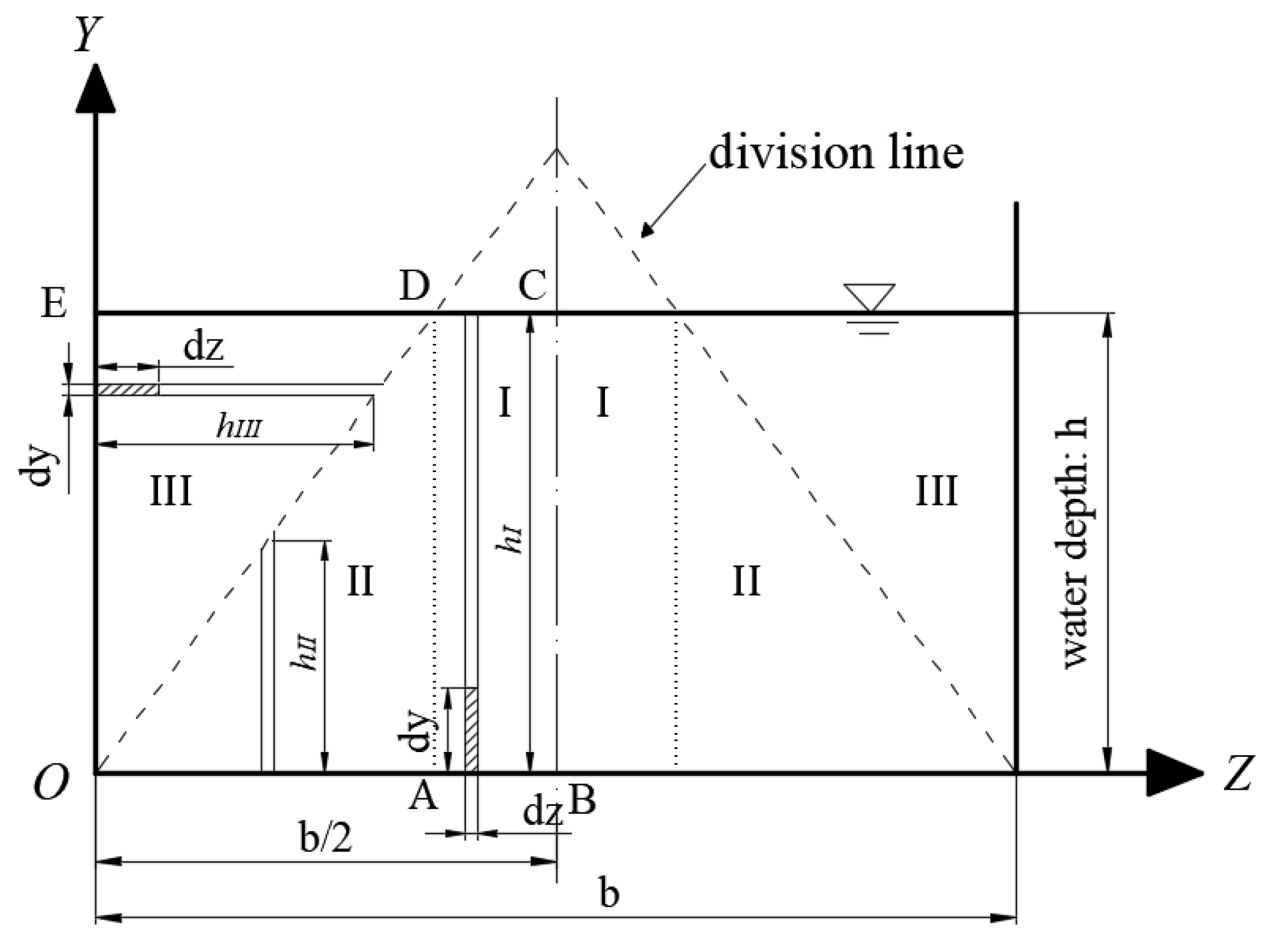
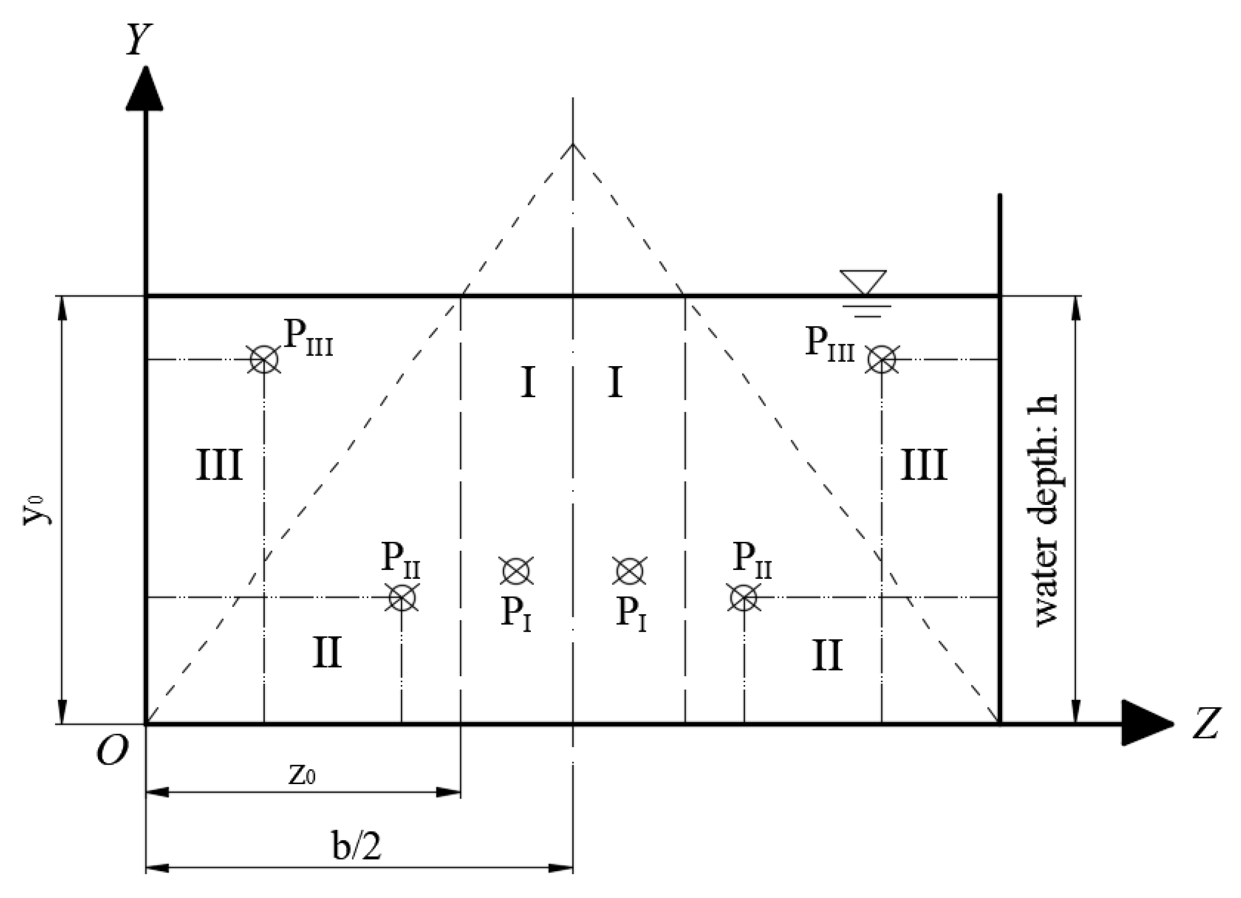
2.1.3. CPL of Regions in Rectangular Channel

For region I, according to Equation (22), since the water depth h in the channel is constant, measuring the velocity of the CPL of depth average velocity can provide the average velocity for the whole section of region I. Therefore, the average discharge can be obtained by multiplying the average cross-section velocity by the area of the region. Similarly, the flow in regions II and III can be obtained using the same method. Figure 3 shows that P_I, P_II, and P_III are the characteristic points that represent the mean velocities in regions I, II, and III, respectively.

For region II, the discharge Q can be expressed using Equation (30):

$$Q=u_{\ast }{\displaystyle {\int }_0^{z_0}\frac{z}{k}}\left(2.5\ln \left(\frac{\sqrt{gS}{\left(\frac{z}{k}\right)}^{1.5}}{e\nu }\right)+5.5\right)dz=\frac{u_{\ast }}{k}\left(z_o{}^2\left(1.25\ln \left(\frac{\sqrt{gS}}{e\nu }{\left(\frac{z_0}{k}\right)}^{1.5}\right)+1.8125\right)\right)$$

(30)

where e is a constant; S is the slope of channel; and z₀ is shown in Figure 3.

The mean velocity can be calculated from the value of Q/A, which can be expressed using Equation (31):

$$\overline{u}=\frac{Q}{A}=\frac{2\frac{u_{\ast }}{k}\left(z_0{}^2\left(1.25\ln \left(\frac{\sqrt{gS}}{e\nu }{\left(\frac{z_0}{k}\right)}^{1.5}\right)+1.8125\right)\right)}{z_0{h}_0}$$

(31)

Using Equations (6), (19) and (31), Equation (32) can be obtained:

$$u_{\ast }\left(2.5\ln \left(\frac{\sqrt{gS}{\left(\frac{z_0}{k}\right)}^{1.5}}{e\nu }\right)+3.625\right)=u_{\ast }\left(2.5\ln \left(\frac{\sqrt{gS}{\left(\frac{z}{k}\right)}^{1.5}}{e\nu }\right)+5.5\right)$$

(32)

Therefore, the y and z value of the point P_II can be calculated using Equation (33):

$$\{\begin{array}{l}\overline{z_{II}}=\frac{z_0}{e^{0.125}}\\ \overline{y_{II}}=\frac{y_0}{e^{1.125}}\end{array}$$

(33)

where $\overline{z_{II}}$ and $\overline{y_{II}}$ represent the coordinates of P_II.

For region III, the analysis method is similar to that of region II. The z and y value of the point P_III, which can be used to calculate the value of Q of region III, can be expressed using Equation (34):

$$\{\begin{array}{l}\overline{z_{III}}=\frac{z_0}{e^{1.125}}\\ \overline{y_{III}}=\frac{y_0}{e^{0.125}}\end{array}$$

(34)

where $\overline{z_{III}}$ and $\overline{y_{III}}$ represent the coordinates of P_III.

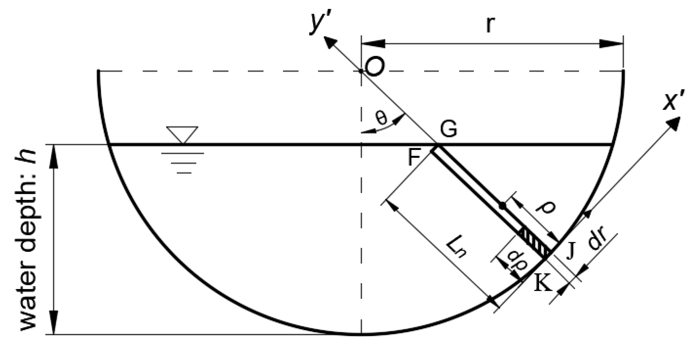
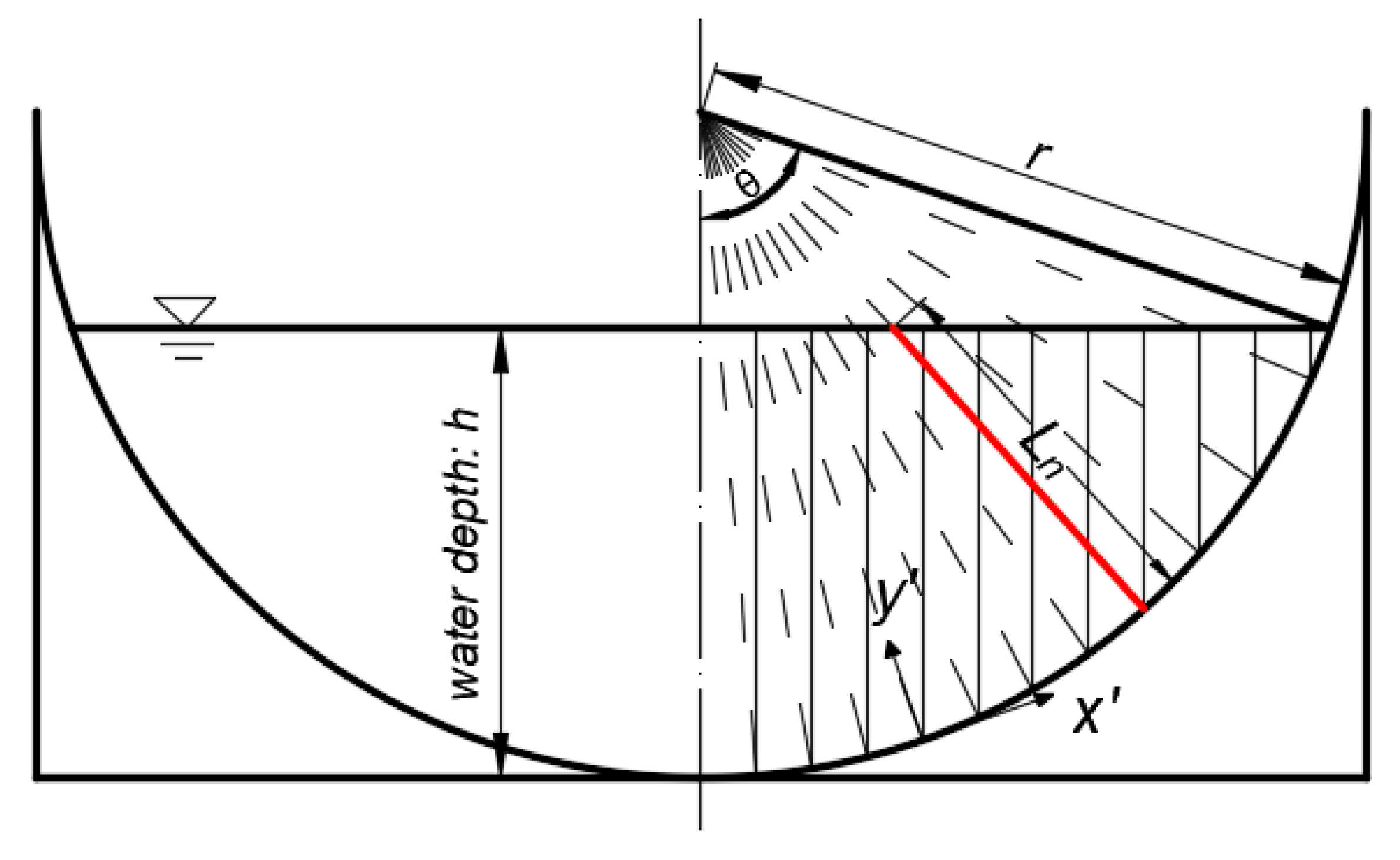
2.2. CPL in Semi-Circular Channel

The concave boundary cross-section is one of the most commonly used cross-section forms in farmland canal systems, open-flow culverts, urban drainage pipelines and other projects. Compared with the rectangular section, it has a larger hydraulic radius under the same conditions, so the velocity of the cross section is larger and the water flow that can be transported is also larger [28]. In order to obtain the discharge of the concave boundary cross-section channel more quickly and accurately, it is necessary to master the velocity distribution of the cross-section. Figure 4 shows the semi-circle channel cross-section.

As shown in Figure 4, a straight line, which crosses the center of the circle and is angled with the center line (θ), is taken from a semicircular channel with radius R and maximum water depth h.

The coordinate system is established by taking the straight line and the direction perpendicular to the straight line as the coordinate axis. According to Figure 4, the rectangle FGJK is L_n in length and dr in width, where Ln is the length of the underwater part of the radius. With the rectangle FGJK, the area is $A_{FGJK}=L_n\cdot dr$ and the discharge through FGJK can be expressed as:

$$Q=u\cdot A_{FGJK}=u\cdot L_n\cdot dr$$

(35)

Then, taking a shadow rectangle whose edge lengths are dρ and dr (dρ and dr are infinitesimal), the discharge through the shadow rectangle is:

$$dQ=u\cdot dr\cdot d\rho$$

(36)

By integrating dρ in the direction of y’ and substituting the log-law, we get:

$$Q=dr\cdot {\displaystyle {\int }_0^{L_n}ud\rho }=dr\cdot u_{\ast }\cdot L_n\cdot \left(2.5\ln \frac{L_n\cdot u_{\ast }}{\nu }+3\right)$$

(37)

Substituting the log-law into Equation (35) gives:

$$Q=L_n\cdot dr\cdot u_{\ast }\cdot \left(2.5\ln \frac{u_{\ast }\cdot \rho }{\nu }+5.5\right)$$

(38)

For Equations (37) and (38), the coordinates of the characteristic points representing the average velocity of the straight line can be obtained from Equation (39):

$$\rho =\frac{L_n}{e}$$

(39)

where ρ is the CPL of the depth average velocity of the line.

2.3. Discharge of Rectangular and Semi-Circular Channel

2.3.1. Discharge in a Rectangular Channel

According to Section 2.1.3, based on the CPLs of different regions, the discharge from the cross-section can be given by Equation (40):

$$Q_{rec}=2\times (A_I{u}_{p_{{}_I}}+A_{II}{u}_{p_{{}_{II}}}+A_{III}{u}_{p_{{}_{III}}})$$

(40)

where A_I, A_II and A_III represent the areas of three regions, and $u_{P_I}$, $u_{P_{II}}$ and $u_{P_{III}}$ represent the velocities of points P_I, P_II, and P_III.

2.3.2. Discharge in a Semi-Circular Channel

Similar to a rectangular channel, in a semi-circle channel, after obtaining the CPL of every normal line, it is necessary to know how to calculate the discharge through simplified point distribution. As shown in Figure 5, two straight lines passing through the center of the circle have divided the angle into θ1, θ2 and θ3. The discharge can be expressed as Equation (41):

$$Q_{cir}=2\times ({\alpha }_c\cdot A_1\cdot u_{CP{L}_1}+A_2\cdot \frac{u_{CP{L}_1}+u_{CP{L}_2}}{2}+{\alpha }_c\cdot A_3\cdot u_{CP{L}_2})$$

(41)

where A₁, A₂ and A₃ represent sub-areas, $u_{CPL}$ is the velocity of the normal line and α_c is the velocity coefficient along the bank. α_c can be determined according to the test conditions.

3. Experimental Setup

Table 1. Summary of experimental conditions.

Cross-Sectional Shape	Conditions	Channel Width: b (m)	Channel Radius: r (m)	Flow Discharge: Q (m3/s)	Water Depth: h (m)
Rectangle	R1 a	0.3	-	0.004	0.065
	R2 a			0.004	0.091
	R3 a			0.004	0.110
	R4 b	0.8	-	0.031	0.120
	R5 b			0.033	0.128
	R6 b			0.039	0.137
	R7 b			0.044	0.153
Semi-circle	S1 c	-	0.120	0.005	0.0813
	S2 c			0.012	0.1200
	S3 a	-	0.150	0.003	0.075
	S4 a			0.005	0.085
	S5 a			0.008	0.100

^a Experiment data are from the Fluid Laboratory of the University of Wollongong(UOW). ^b Experiment data are from the Hydraulic Experiment Hall of China Agricultural University(CAU). ^c Experiment data are from Knight [29].

summarizes the test conditions and relevant parameters of a channel cross-section. The rectangle and semi-circle channel section tests are shown in the table. In order to increase the reliability of the test data, the tests are carried out in different places, such as the Fluid Laboratory of the University of Wollongong, the Hydraulic Experiment Hall of the China Agricultural University and the Semi-Circular Test Open Channel of the British Council for Scientific and Engineering Research [29]. Different groups were set up by changing the discharge (or water depth) of the channel. Using acoustic doppler velocimetry (ADV) and other velocity measurement tools to measure the vertical velocity of a cross-section, a large amount of velocity data can be obtained.

4. Results and Discussion

4.1. Analysis with Rectangular Channels

The consistency of CPL of R1, R2 and R3 in rectangular channels is analyzed in Figure 6. These scatter points cover three regions of the rectangular cross-section. The abscissa of the scatter points in the figure represents the theoretical value of CPL and is calculated by Equations (22), (23) and (29). The longitudinal coordinates of points represent the measured value of CPL, which can be obtained by interpolating the experimental data. It can be seen that the data points are mostly distributed within the error line of ±15%. Therefore, it can be proven that the formulas of CPL in Section 2.1.2 can be applied to rectangular cross-section channels.

In order to further verify the correctness of the theoretical derivation, a series of experiments were conducted at different water depths at the CAU (China). We collated the experimental data of R4-R7 and selected the representative data points to draw in Figure 7. Since the perpendicular bisector is in region I, we calculated the point of CPL with Equation (22). Since the number of measuring points was less, and there were some test errors, the relative error between CPLt and CPLm still existed. With the increase in water depth, the influence of several measuring points on the results is apparent (R7). The velocities of CPLt and CPLm have a greater consistency when the number of measuring points is high. Hence, we have reason to think that the velocity of CPLt can represent the average velocity of the centerline in rectangular channels.

The characteristic points of depth average velocity in each region are plotted in Figure 8 and recorded as PI, PII and PIII, which are calculated by Equations (22), (33) and (34), respectively. We can obtain the discharge by using the values of PI, PII and PIII in Equation (40). Curves in the graph are isovel patterns in the rectangular cross-section channel based on UOW test data, which is consistent with the contour line measured by Chiu and Chiou [30]. It can be seen from the figures that the velocity near the wall is small and the velocity far from the wall is large. This can be explained by the log-law of velocity distribution. Increasing the monotone leads to the velocity increasing as the distance from the channel side wall or bed increases. Therefore, the maximum velocity point of the cross-section should theoretically be located at the intersection of the vertical line of the channel and the water surface.

However, in Figure 8, we can see that the maximum velocity point is below the water surface, not on it. This phenomenon was first observed about a century ago [31,32], and further experimental studies showed that it was induced by the presence of secondary cross-sectional flow structures [33]. Due to the occurrence of anisotropic turbulence and cross-sectional secondary currents, which tend to shift the maximum velocity from the free surface to the bed, its identification is still a complex task in hydraulics [34].

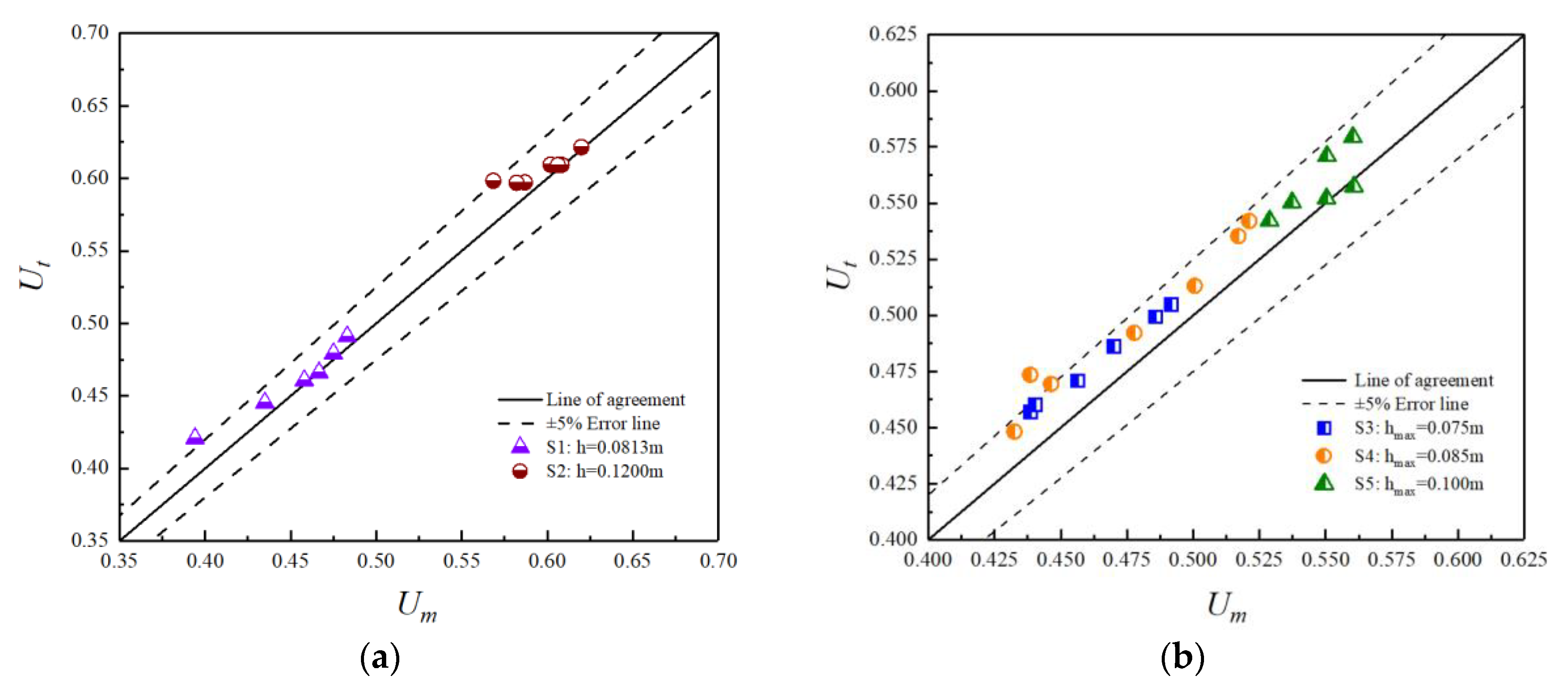
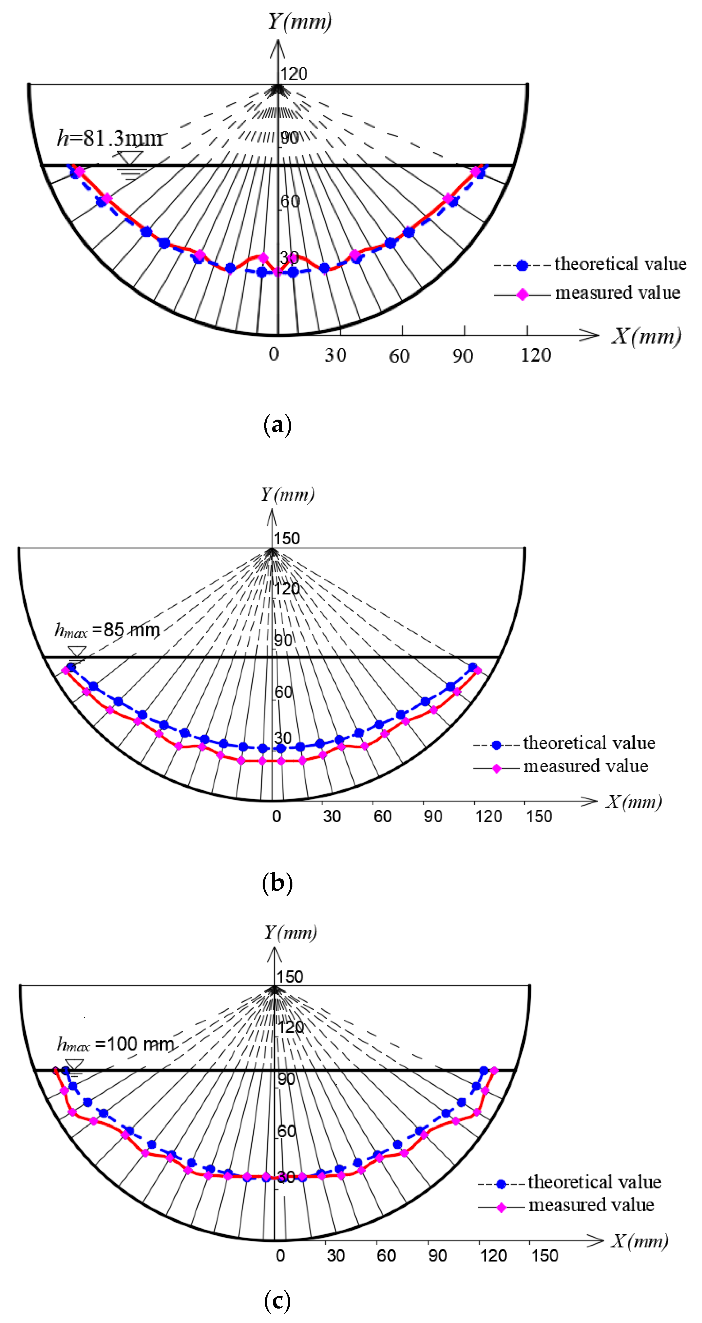
4.2. Analysis with Semi-Circular Channels

Mechanical energy is always transmitted to the closest boundary. As shown in Figure 9, this refers to the normal line direction. So, in a concave boundary channel, the analysis is carried out along the normal direction perpendicular to the tangent direction of the wall.

In order to compare the accuracy of velocity distribution analysis along the vertical direction and along the normal wall direction, the following analysis has been made. The error values obtained by the experimental condition S2 (in Table 1) and log-law formulas are compared in tabular analysis in

Table 2. Accuracy comparison of velocity distribution along the vertical wall and normal directions with S2: h = 0.1200.

Average Error Value along Normal Direction		Average Error Value along Vertical Direction
Normal Slope kn	Average Error Value E (%)	The Distance from the Vertical Line to the Central Line z/b	Average Error Value E (%)
11.9	2.156661	0.083	3.528655
5.91	3.117373	0.167	3.441878
3.87	2.578154	0.250	2.827718
2.82	3.073467	0.333	7.846099
2.18	3.217222	0.417	6.557529
1.73	2.584048	0.500	10.55338
1.39	2.047317	0.583	12.39980
1.11	2.207014	0.667	19.05022
0.88	2.758453	0.750	21.84237
0.66	4.707039	0.833	30.18244

. The calculation formula of the average error value is given by:

$$E=\frac{E_m-E_c}{E_m}\times 100\%$$

(42)

where E is the average error value in Table 2, E_m denotes the measured value, and E_c denotes the calculated value.

From Table 2, we can conclude that the average error value obtained by normal analysis along the wall is much lower than that obtained by vertical analysis when consistency analysis of the velocity measurements and the log-law is carried out. Hence, the correctness of the analysis of the concave boundary channel along the normal direction perpendicular to the wall is proved.

Figure 10 shows the comparison of average velocity along the normal line under S1−S5. The horizontal ordinates in the figure are the average value of the velocity at each normal measuring line. The vertical coordinates are obtained by theoretical calculation. Specifically, the CPL is calculated by the formula from Section 2.2, and then the average velocity on the normal line is obtained by substituting it into the log-law.

Despite some fluctuations of a few test points in Figure 10, most of them are within the error range of 5%. The statistical rules of a large number of test points can still prove the accuracy of the theoretical deduction in Section 2.2. Therefore, the velocity corresponding to the CPL calculated by Equation (39) can represent the average velocity of the channel wall along the normal line to the water surface line. Most points, especially the measuring points close to the water surface, are located above the agreement line, which implies that U_t is bigger than U_m. This is because the log-law appears to deviate near the water surface. Based on this, the log-wake law was proposed by Coles [35], which appears to be the most reasonable extension of the log-law. However, the value of Π in the log-wake law seems not to be universal [36]. So, more research is needed to correct the velocity near the water surface.

As shown in Figure 11, the theoretical and measured values of CPL on each normal line are very close, located in the middle and lower part of the normal line. The solid and dotted lines are smooth arc curves, which are consistent with the concave boundary. Therefore, the accuracy of the formula in Section 2.2 can be proved. It is advisable to use the velocity of CPL to represent the average velocity of the normal line.

When the S1 condition is applied to Equation (41), we can calculate the discharge of the semi-circular channel. Here, α_c = 0.8.

Table 3. Analysis of calculated and measured discharge under different combinations of angles (S1).

Degree of Angle with the Two-Line Method			Q Calculation (m3/s)	Q Measurement (m3/s)	Relative Error (%)
θ1 (°)	θ2 (°)	θ3 (°)
71/3	71/3	71/3	0.00526	0.005	5.10
18	34	19	0.00565		12.90
18	23	30	0.00531		6.27
29	32	10	0.00551		10.09
35	26	10	0.00542		8.48
36	21	14	0.00533		6.61

shows the calculated discharge of the channel with the combination of six kinds of angles. Only the first is a uniform partition; the others are all non-uniform. Relative error refers to the error value of the calculated discharge relative to the measured discharge. It can be found that the relative error value is the smallest only when the angle is divided uniformly, about 5%. Therefore, we can reasonably conclude that the accuracy of the discharge calculation is the highest only if the angle is divided uniformly while using the two-line method.

5. Summary

This study has investigated a fast flow measurement method based on the distribution of measuring points by conducting laboratory experiments. The principal achievements from the comparison of the theoretical derivation and experimental study are summarized below.

(1)

Based on Yang et al.’ s partitioning theory [21,22,27], this paper gives a re-description of the existing form of the division line of a rectangular cross-section channel. That is, whether the channel cross-section is wide–shallow or narrow–deep with the center line of the cross-section as the symmetrical axis, and whether the intersection points of the left and right division lines intersect on or above the water surface.

(2)

This paper analyzes characteristic points in flat channels (e.g., rectangular channel) and concave boundary channels (e.g., semi-circular channel). In the rectangular channel, the division line divides the section into three regions. In each region, the analysis is conducted in the direction perpendicular to the bottom or side wall of the channel. In the semi-circular channel, the analysis is conducted along the normal direction. Based on the log-law, the theoretical expressions for calculating the location of the average velocity characteristic points in flat and concave boundary channels are derived through the formula transformation.

(3)

The velocity data in different experimental sites are used to verify the validity of the CPL formulas applied to flat and concave boundary channels. Moreover, the discharge calculation formulas of channels are given through discussion with CPL.

6. Conclusions

The determination of CPL has provided a theoretical basis for simplifying and accurately measuring channel flow. It is precisely because of the realization of CPL that the average cross-section discharge can be calculated quickly so that the accuracy and stability of flow measurement in irrigation channels can be further improved.

The results of this paper can only serve for smooth open channels. However, if the roughness is non-uniform, the location of the division lines in the channel cross-section will be different [25]. It is also difficult to ensure that the velocity distribution in each sub-region is the same. With the comprehensive ecological treatment of channels becoming a hot topic, the transition from smooth channels to vegetation covered channels becomes relevant. So, it is of necessity to conduct experiments in open channels with roughness for future research.

References

1. Mancosu, N.; Snyder, R.L.; Kyriakakis, G.; Spano, D. Water Scarcity and Future Challenges for Food Production. Water 2015, 7, 975–992. [Google Scholar] [CrossRef]
2. Salehi, S.; Azimi, A.H. Discharge Characteristics of Weir-Orifice and Weir-Gate Structures. J. Irrig. Drain. Eng. 2019, 145. [Google Scholar] [CrossRef]
3. Samani, Z. Three simple flumes for flow measurement in open channels. J. Irrig. Drain. Eng. 2017, 143. [Google Scholar] [CrossRef]
4. Samani, Z.; Magallanez, H. Simple flume for flow measurement in open channel. J. Irrig. Drain. Eng. 2000, 126, 127–129. [Google Scholar] [CrossRef]
5. Keulegan, G.H. Laws of turbulent flow in open channels. J. Res. Natl. Bur. Stand. 1938, 21, 707–741. [Google Scholar] [CrossRef]
6. Zanoun, E.-S.; Durst, F.; Bayoumy, O.; Al-Salaymehc, A. Wall skin friction and mean velocity profiles of fully developed turbulent pipe flows. Exp. Therm. Fluid. Sci. 2007, 32, 249–261. [Google Scholar] [CrossRef]
7. Nikuradse, J. Laws of Flow in Rough Pipes (1950 translation); National Advisory Committee for Aeronautics: Washington, DC, USA, 1933; NACA-TM-1292. Available online: https://ntrs.nasa.gov/search.jsp?R=19930093938 (accessed on 15 January 2020).
8. Cardoso, A.H.; Graf, W.H.; Gust, G. Uniform-Flow in a Smooth Open Channel. J. Hydraul. Res. 1989, 27, 606–616. [Google Scholar] [CrossRef]
9. Steffler, P.M.; Rajaratnam, N.; Peterson, A.W. LDA Measurements in Open Channel. J. Hydraul. Eng.-ASCE 1985, 111. [Google Scholar] [CrossRef]
10. Nezu, I.; Rodi, W. Open-Channel Flow Measurements with a Laser Doppler Anemometer. J. Hydraul. Eng. 1986, 112, 335–355. [Google Scholar] [CrossRef]
11. Chiu, C.L. Entropy and 2-D velocity distribution in open channels. J. Hydraul. Eng. 1988, 114, 738–756. [Google Scholar] [CrossRef]
12. Chiu, C.L. Application of entropy concept in open-channel flow study. J. Hydraul. Eng. 1991, 117, 615–628. [Google Scholar] [CrossRef]
13. Chiu, C.L.; Murray, D.W. Variation of velocity distribution along non-uniform open-channel flow. J. Hydraul. Eng. 1992, 118, 989–1001. [Google Scholar]
14. Maghrebi, M.F. Application of the single point measurement in discharge estimation. Adv. Water Resour. 2006, 29, 1504–1514. [Google Scholar] [CrossRef]
15. Bretheim, J.U.; Meneveau, C.; Gayme, D.F. Standard logarithmic mean velocity distribution in a band-limited restricted nonlinear model of turbulent flow in a half-channel. Phys. Fluids 2015, 27. [Google Scholar] [CrossRef] [Green Version]
16. Hong, J.H.; Guo, W.D.; Wang, H.W.; Yeh, P.H. Estimating discharge in gravel-bed river using non-contact ground-penetrating and surface-velocity radars. River Res. Appl. 2017, 33, 1177–1190. [Google Scholar] [CrossRef]
17. Moramarco, T.; Barbetta, S.; Tarpanelli, A. From Surface Flow Velocity Measurements to Discharge Assessment by the Entropy Theory. Water 2017, 9, 120. [Google Scholar] [CrossRef] [Green Version]
18. Johnson, E.D.; Cowen, E.A. Estimating bed shear stress from remotely measured surface turbulent dissipation fields in open channel flows. Water Resour. Res. 2017, 53, 1982–1996. [Google Scholar] [CrossRef]
19. Johnson, E.D.; Cowen, E.A. Remote determination of the velocity index and mean streamwise velocity profiles. Water Resour. Res. 2017, 53, 7521–7535. [Google Scholar] [CrossRef] [Green Version]
20. Khuntia, J.R.; Kamalini, D.; Khatua, K.K. Prediction of depth-averaged velocity in an open channel flow. Appl. Water Sci. 2018, 8, 172. [Google Scholar] [CrossRef] [Green Version]
21. Han, Y.; Yang, S.Q.; Dharmasiri, N.; Sivakumar, M. Experimental study of smooth channel flow division based on velocity distribution. J. Hydraul. Eng. 2015, 141. [Google Scholar] [CrossRef]
22. Yang, S.Q.; Han, Y.; Lin, P.Z.; Jiang, C.B.; Walker, R. Experimental study on the validity of flow region division. J. Hydro-Environ. Res. 2014, 8, 421–427. [Google Scholar] [CrossRef] [Green Version]
23. Melling, A.; Whitelaw, J.H. Turbulent flow in a rectangular duct. J. Fluid Mech. 1976, 78, 289–315. [Google Scholar] [CrossRef]
24. Tracy, H.J. Turbulent flow in a three-dimensional channel. J. Hydraul. Div. 1965, 91, 9–35. [Google Scholar]
25. Einstein, H.A. Formulas for the transportation of bed load. Trans. ASCE 1942, 107, 133–169. [Google Scholar]
26. Chien, N.; Wang, Z. Mechanics of Sediment Transport; Science Press: Beijing, China, 1986. (In Chinese) [Google Scholar]
27. Yang, S.Q.; Lim, S.Y. Mechanism of energy transportation and turbulent flow in a 3D channel. J. Hydraul. Eng.-ASCE 1997, 123, 684–692. [Google Scholar] [CrossRef]
28. Luo, J. Study on the Hydraulic Characteristics of Pressure-Free Uniform Flow in Circular Section Pipeline. Master’s Thesis, Tsinghua University, Beijing, China, 2016. (In Chinese). [Google Scholar]
29. Knight, D.W.; Sterling, M. Boundary shear in circular pipes running partially full. J. Hydraul. Eng.-ASCE 2000, 126, 263–275. [Google Scholar] [CrossRef]
30. Chiu, C.L.; Chiou, J.D. Structure of 3-D flow in rectangular open channels. J. Hydraul. Eng.-ASCE 1986, 112, 1050–1068. [Google Scholar] [CrossRef]
31. Stearns, F.P. A reason why the maximum velocity of water flowing in open channels is below the surface. Trans. Am. Soc. Civ. Eng. 1883, 7, 331–338. [Google Scholar]
32. Murphy, C. Accuracy of stream measurements. Water Supply Irrig. 1904, 95, 111–112. [Google Scholar]
33. Tominaga, A.; Nezu, I. Turbulent structure in compound open-channel flows. J. Hydraul. Eng.-ASCE 1991, 117, 21–41. [Google Scholar] [CrossRef]
34. Mirauda, D.; Pannone, M.; De Vincenzo, A. An Entropic Model for the Assessment of Streamwise Velocity Dip in Wide Open Channels. Entropy. 2018, 20, 69. [Google Scholar] [CrossRef] [Green Version]
35. Coles, D. The Law of the Wake in the Turbulent Boundary Layer. J. Fluid Mech. 1956, 1, 191–226. [Google Scholar] [CrossRef] [Green Version]
36. Absi, R. An ordinary differential equation for velocity distribution and dip-phenomenon in open channel flows. J. Hydraul. Res. 2011, 49, 82–89. [Google Scholar] [CrossRef]
Figure 1. Division lines for smooth rectangular channels: (a) b/hα; (b) b/hα.
Water 12 00430 g001
Figure 2. Flow partitioning in rectangular channels.
Water 12 00430 g002
Figure 3. Location map of the characteristic points in different regions.
Water 12 00430 g003
Figure 4. Section diagram of semi-circular channel.
Water 12 00430 g004
Figure 5. Discharge calculation in a semi-circular channel with the two-line method.
Water 12 00430 g005
Figure 6. Comparison of the CPL between the theoretical and measured values in a rectangular channel.
Water 12 00430 g006
Figure 7. Velocity on the perpendicular bisector with R4-R7 in a rectangular channel.
Water 12 00430 g007
Figure 8. Isovel patterns in a rectangular channel (e.g. R1: b/h = 4.615).
Water 12 00430 g008
Figure 9. Semi-circular channel cross-section and notation.
Water 12 00430 g009
Figure 10. Comparison of measured and theoretical values of mean radial velocity (a) S1, S2; (b) S3, S4, S5.
Water 12 00430 g010
Figure 11. Comparison of measured and theoretical values of CPL (a) S1; (b) S4; (c) S5.
Water 12 00430 g011