Trend Analyses of Meteorological Variables and Lake Levels for Two Shallow Lakes in Central Turkey

Abstract

Trend analyses of meteorological variables play an important role in assessing the long-term changes in water levels for sustainable management of shallow lakes that are extremely vulnerable to climatic variations. Lake Mogan and Lake Eymir are shallow lakes offering aesthetic, recreational, and ecological resources. Trend analyses of monthly water levels and meteorological variables affecting lake levels were done by the Mann-Kendall (MK), Modified Mann-Kendall (MMK), Sen Trend (ST), and Linear trend (LT) methods. Trend analyses of monthly lake levels for both lakes revealed an increasing trend with the Mann-Kendall, Linear, and Sen Trend tests. The Modified Mann-Kendall test results were statistically significant with an increasing trend for Eymir lake levels, but they were insignificant for Mogan lake due to the presence of autocorrelation. While trend analyses of meteorological variables by Sen Test were significant at all tested variables and confidence levels, Mann-Kendall, Modified Mann-Kendall, and Linear trend provided significant trends for only humidity and wind speed. The trend analyses of Sen Test gave increasing trends for temperature, wind speed, cloud cover, and precipitation; and decreasing trends for humidity, sunshine duration, and pan evaporation. These results show that increasing precipitation and decreasing pan evaporation resulted in increasing lake levels. The results further demonstrated an inverse relationship between the trends of air temperature and pan evaporation, pointing to an apparent “Evaporation Paradox”, also observed in other locations. However, the increased cloud cover happens to offset the effects of increased temperature and decreased humidity on pan evaporation. Thus, all relevant factors affecting pan evaporation should be considered to explain seemingly paradoxical observations.

1. Introduction

Lakes are valuable water resources for humans, playing important roles in aquatic and terrestrial ecosystems and the environment [1,2,3,4]. Owing to the combined impact of anthropogenic activities and climatic variation, many lakes around the world are under threat [5,6]. Global climate change and anthropogenic activities adversely affect both water quantity and quality, having a critical influence on regional sustainable development. Water level fluctuation, a sensitive marker of change, is an important driver for lakes, with an impact on lake ecosystems [7]. Therefore, determination and understanding of long-term changes in water levels due to climatic variables are necessary to establish sustainable management of lakes.

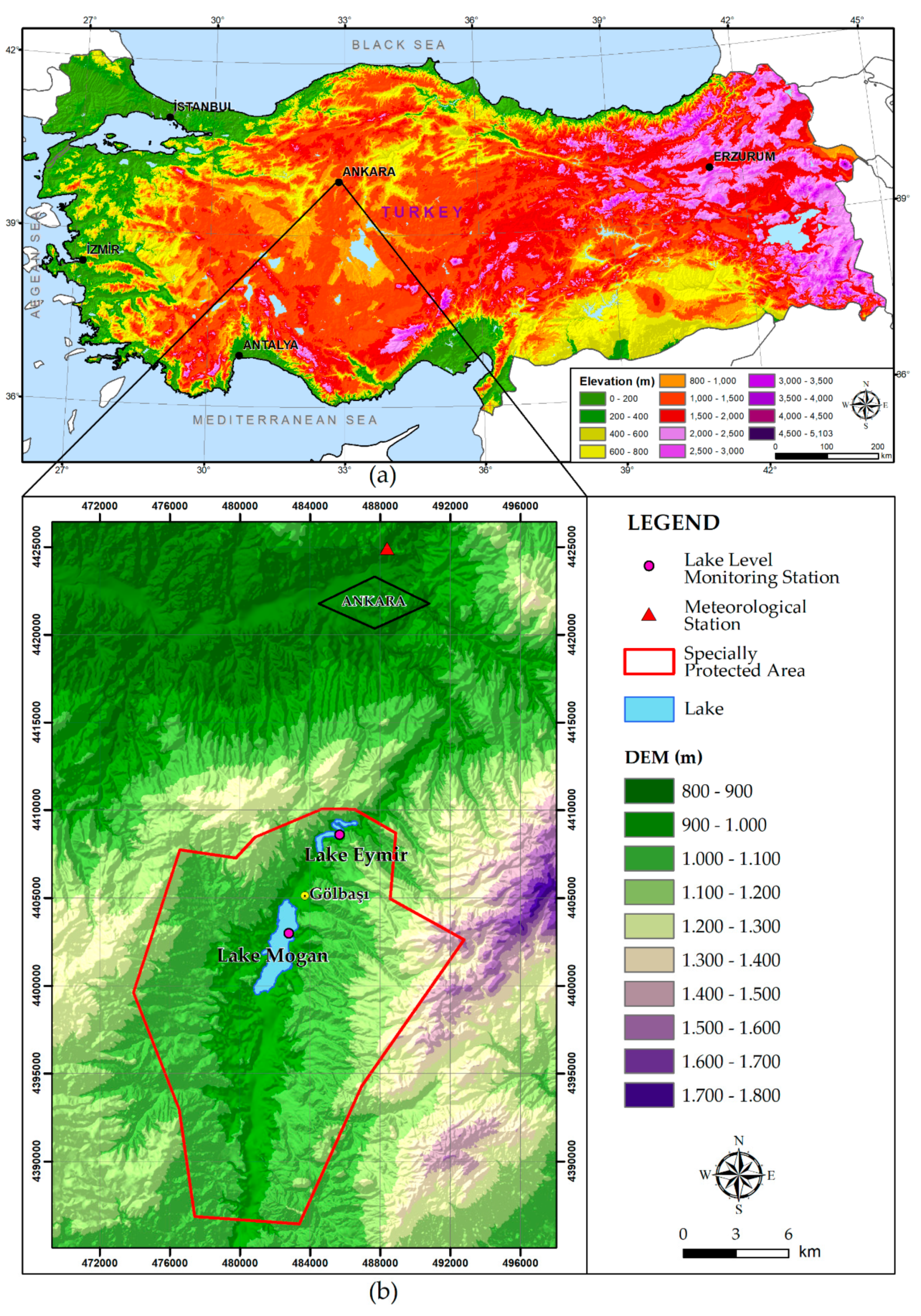
Shallow lakes Mogan and Eymir, located 20 km south of Ankara in Central Turkey, are important aesthetic, recreational, and ecological resources for the city of Ankara and the town of Gölbaşı (Figure 1). The drainage area of Lake Mogan is 926 km² and that of Lake Eymir is 42 km². Although both lakes and their surrounding areas mainly meet urban housing and recreational needs, the wildlife and biodiversity values of the lakes are high. These lakes, especially Lake Mogan, have wetlands housing more than 26 mammal species and 231 bird species, 76 of which are breeding. Hydrologically connected lakes are designated as ‘‘Specially Protected Areas’’, and Lake Mogan was declared as an ‘‘Important Bird Area’’ in 1990 by the Ministry of Environment and Urbanization. Because of their importance, there is a growing concern about the possible impacts of climate change on the long-term sustainability of these lakes [8].

Although trends in lake levels of Turkey’s five largest lakes (İznik, Eğirdir, Tuz, Beyşehir, and Van lake) were analyzed using Mann-Kendall and Sen tests [9], there is no existing study on the hydrologic relationship between the trends of lake levels and meteorological variables. Therefore, the emphasis in this research is on the determination and quantification of trends in monthly lake water levels and hydrometeorological variables (average monthly pan evaporation, air temperature (°C), precipitation (mm), humidity (%), wind speed (m/s), cloud cover (8 okta), and sunshine duration (h)). This will enable researchers to investigate the effect of changes in hydrometeorological variables on the water levels of Lake Mogan and Lake Eymir. The analyses were conducted by using four methods: Mann-Kendall (MK), Modified Mann-Kendall (MMK), Sen Trend (ST), and Linear trend (LT). Trends at 90%, 95%, and 99% confidence levels were examined and compared. Understanding long-term trends in hydrometeorological variables are of high significance for sustainable water resource management [10].

2. Materials and Methods

Meteorological variables change in time and space for many reasons. These changes, based on observations, should be investigated through statistical methods. Trend analysis is the most important statistical method widely used around the world to assess the long-term changes in time series of meteorological variables, such as precipitation, temperature, evaporation, etc. [8,11,12,13,14,15,16,17].

The aim of this study was to evaluate the long-term trends of monthly water levels and meteorological variables affecting lake levels (average monthly pan evaporation, air temperature (°C), precipitation (mm), humidity (%), wind speed (m/s), cloud cover (8 okta), and sunshine duration (h)) through Mann-Kendall (MK), Modified Mann-Kendall (MMK), Sen Trend (ST), and Linear trend (LT) statistical methods at confidence levels of 90%, 95%, and 99%. The meteorological data and lake levels between 1997 and 2015 were obtained from Ankara Meteorology General Directorate and State Hydraulic Works, respectively. Unfortunately, these lake levels have not been monitored post 2015. Hence, the period selected for trend analysis was as per the lake monitoring duration.

Table 1. Location information of observation stations.

Station Name	Coordinates *		Elevation (m)
	South (m)	East (m)
17130/Ankara	488,396	4,424,913	891
Lake Eymir	485,674	4,408,599	968
Lake Mogan	482,787	4,402,980	972

* ED50/UTM Zone 36N.

provides location information of the Ankara meteorological station and lake level monitoring stations utilized in the study.

Table 2. Statistical characteristics of the variables.

Station	Parameters	Min	Max	Mean	Sx	Csx
Ankara 17130	Average Monthly Temperature (°C)	−3.85	28.45	12.89	8.55	0.01
	Monthly Total Precipitation (mm)	0.00	167.60	34.41	27.07	1.23
	Average Monthly Humidity (%)	28.07	87.07	59.74	12.90	−0.25
	Average Monthly Wind Speed (m/s)	1.24	3.79	2.29	0.46	0.58
	Monthly Total Sunshine Duration (h)	42.5	399.20	199.12	96.37	0.04
	Monthly Total Evaporation (mm)	62.6	357.90	151.93	80.92	0.03
	Average Monthly Cloud Cover (8 okta)	0.5	6.80	3.24	1.34	0.06
Eymir	Average Monthly Lake Level (m)	966.38	969.5	968.24	0.78	−0.37
Mogan	Average Monthly Lake Level (m)	971.79	974.3	972.81	0.46	0.10

Sx: Standard deviation, Csx: Skewness coefficient.

shows the statistical characteristics of the variables used in the study.

2.1. Mann-Kendall (MK)

The non-parametric Mann-Kendall test may be used to detect trends that are monotonic, but not necessarily linear. This method tests if there is a trend in the time series data [18,19,20]. It is a non-parametric rank-based procedure, robust to the influence of extremes and suitable for application with skewed variables [11]. Test statistics are:

$$\mathrm{sgn}({\mathrm{x}}_{\mathrm{j}}-{\mathrm{x}}_{\mathrm{i}})=\{\begin{array}{ccc}1;& \mathrm{if}& {\mathrm{x}}_{\mathrm{j}}>{\mathrm{x}}_{\mathrm{j}}\\ 0;& \mathrm{if}& {\mathrm{x}}_{\mathrm{j}}={\mathrm{x}}_{\mathrm{i}}\\ -1;& \mathrm{if}& {\mathrm{x}}_{\mathrm{j}}<{\mathrm{x}}_{\mathrm{i}}\end{array}$$

(1)

In Equation (1), x_i and x_j are the data values in time series i and j, respectively, and in Equation (2), n is the number of data points, sgn (x_j − x_i) is the sign function as:

$$\mathrm{S}={\displaystyle \sum _{\mathrm{i}=1}^{\mathrm{n}-1}{\displaystyle \sum _{\mathrm{j}=\mathrm{i}+1}^{\mathrm{n}}\mathrm{sgn}({\mathrm{x}}_{\mathrm{j}}-{\mathrm{x}}_{\mathrm{i}})}}$$

(2)

The variance is computed as:

$$\mathrm{Var}(\mathrm{S})=\frac{\mathrm{n}(\mathrm{n}-1)(2\mathrm{n}+5)-{\displaystyle \sum _{\mathrm{i}=1}^{\mathrm{P}}{\mathrm{t}}_{\mathrm{i}}({\mathrm{t}}_{\mathrm{i}}-1)(2{\mathrm{t}}_{\mathrm{i}}+5)}}{18}$$

(3)

In Equation (3), n refers to the number of data, P shows the number of tied groups, and t_i indicates the number of ties of extent i. A tied group is a set of sample data and has the same value. In case sample size n > 10, the standard normal test statistic Z is calculated using Equation (4):

$$\mathrm{Z}=\{\begin{array}{ccc}\frac{\mathrm{S}-1}{\sqrt{\mathrm{Var}(\mathrm{S})}};& \mathrm{if}& \mathrm{S}>0\\ 0& \mathrm{if}& \mathrm{S}=0\\ \frac{\mathrm{S}+1}{\sqrt{\mathrm{Var}(\mathrm{S})}}& \mathrm{if}& \mathrm{S}<0\end{array}$$

(4)

The computed standard Z value is compared with standard normal distribution according to two-tailed confidence levels (α = 10%, α = 5%, α = 1%). If the computed Z value is greater than |Z| ≥ |Z_{1 − α/2}|, the null hypothesis (H₀) is rejected and thus the H_a (alternative hypothesis) hypothesis is accepted. In this study, two-tailed confidence levels (α = 10%, α = 5% and α = 1%) are used for the Mann-Kendall trend test [12].

2.2. Modified Mann-Kendall (MMK)

The modified Mann-Kendall (MMK) method is a modified nonparametric trend method suitable for autocorrelated data based on the modified value in the variance of the test statistic. The accuracy of the modified test in terms of empirical significance was found to be superior to the original Mann-Kendall trend test without any loss of power. In the MMK test, the effect of autocorrelation on the calculated variance value is also considered. Adjusted variance expression is calculated as given below and Z values are found with the help of Equations (5) and (6) [13]:

$$\mathrm{V}(\mathrm{S})=\mathrm{Var}(\mathrm{S})\times \frac{\mathrm{n}}{{\mathrm{n}}_{\mathrm{s}}^{*}}=\frac{\mathrm{n}(\mathrm{n}-1)(2\mathrm{n}+5)}{18}\times \frac{\mathrm{n}}{{\mathrm{n}}_{\mathrm{s}}^{*}}$$

(5)

$$\frac{\mathrm{n}}{{\mathrm{n}}_{\mathrm{s}}^{*}}=1+\frac{2}{\mathrm{n}(\mathrm{n}-1)(\mathrm{n}-2)}\times {\displaystyle \sum _{\mathrm{i}=1}^{\mathrm{n}-1}(\mathrm{n}-\mathrm{i})}(\mathrm{n}-\mathrm{i}-2){\mathsf{\rho }}_{\mathrm{s}}(\mathrm{i})$$

(6)

Where n/n_s*, represents a correction due to autocorrelation in the data. “n” is the actual number of observations and ρ_s(i) is the autocorrelation of the observation ranks.

2.3. Linear Trend (LT)

Linear trend analysis is a commonly used method to determine the tendency in a hydrological time series. It is based on the solution of the graph obtained by writing two different variables on separate axes. It is necessary to fit a line that best expresses the distribution of the time series and determine the curve of this line [14,15].

$$\mathrm{Y}={\mathsf{\beta }}_0+{\mathsf{\beta }}_1\mathrm{X}$$

(7)

In Equation (7), β₀ is a constant value and β₁ is the slope. If this equation is used in the determination of trend analysis, β₁ is expressed as the amount of decrease or increase on trend [16]. If the variable data show a statistically significant trend determined by the t-test, t value of the β₁ value (inclination) is calculated with the help of Equation (7). “t_cal” is compared with a selected confidence level (e.g., α =5 %). If it exceeds the confidence level (critical level), there is a trend and is in an ascending or descending direction relative to the sign. If it does not exceed (−t_cri < t_cal < t_cri), there is no statistically significant trend [17].

2.4. Sen Trend (ST)

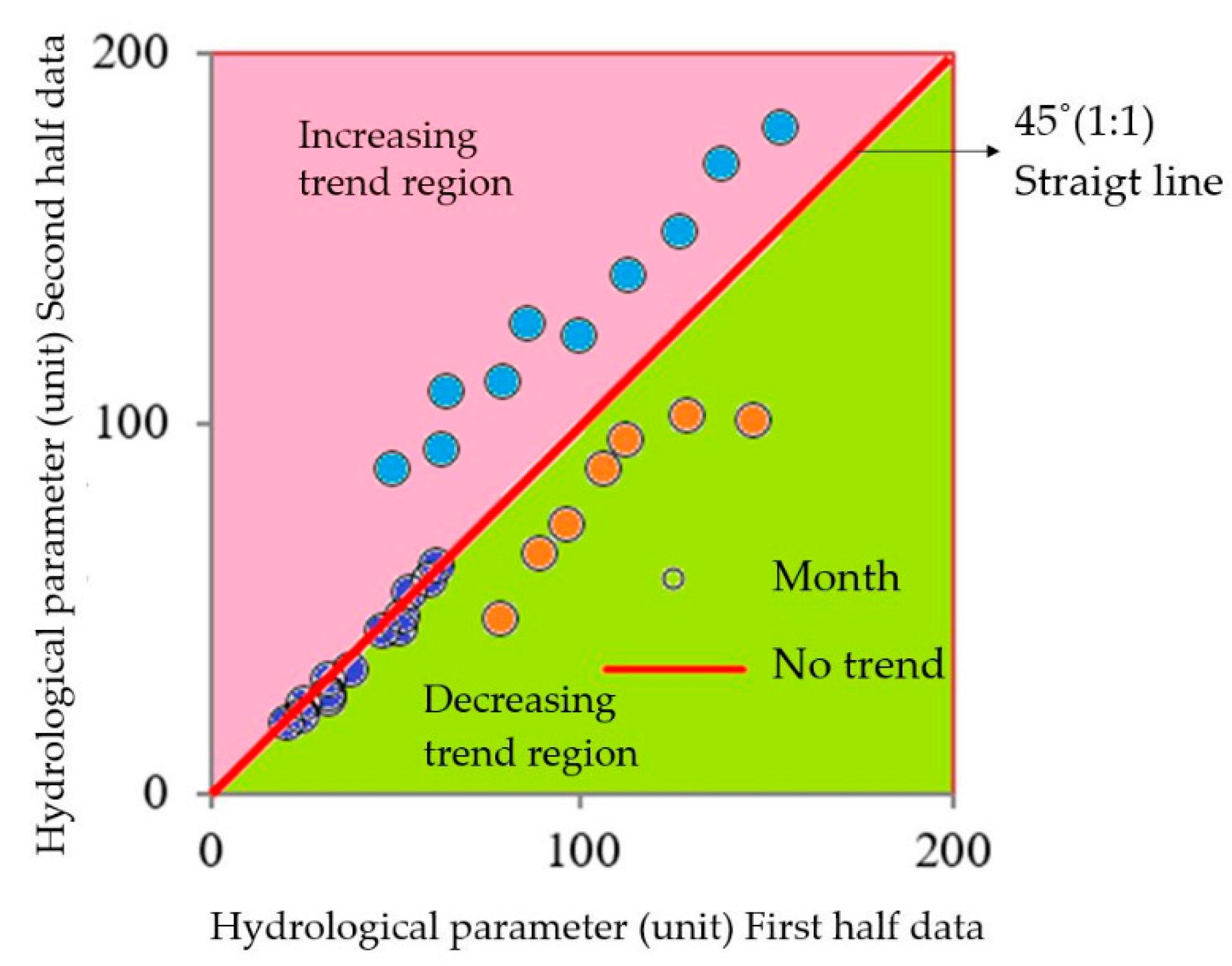
In this method, first, time series is divided into two halves. Each sub-series are sorted in an ascending manner. Then, the first sub-series (X_i) are located on the X-axis, and the other sub-series (X_j) are located on the Y-axis in the Cartesian coordinate system (Figure 2). If data are collected on the 1:1 (45°) straight line, it can be said that there is no trend (a trendless time series). If data are accumulated in the triangular area below the 1:1 (45°) straight line, there is a decreasing trend. If data are accumulated in the upper triangular area of the 1:1 (45°) straight line, there is an increasing trend [21,22,23]. Moreover, low, medium, and high values of a variable can be graphically evaluated with this method.

Sen developed a new statistical process using this method [23]; its steps are shown in Equations (8)–(12):

$$\mathrm{E}(\mathrm{s})=\frac{2}{\mathrm{n}}\left[\mathrm{E}({\overline{\mathrm{y}}}_2)-\mathrm{E}({\overline{\mathrm{y}}}_1)\right]$$

(8)

$${\mathsf{\sigma }}_{\mathrm{s}}^2=\frac{4}{{\mathrm{n}}^2}\left[\mathrm{E}({\overline{\mathrm{y}}}_2^2)-2\mathrm{E}({\overline{\mathrm{y}}}_2{\overline{\mathrm{y}}}_1)-\mathrm{E}({\overline{\mathrm{y}}}_1^2)\right]$$

(9)

$${\mathsf{\rho }}_{{\overline{\mathrm{y}}}_2{\overline{\mathrm{y}}}_1}=\frac{\mathrm{E}({\overline{\mathrm{y}}}_2{\overline{\mathrm{y}}}_1)-\mathrm{E}({\overline{\mathrm{y}}}_2)-\mathrm{E}({\overline{\mathrm{y}}}_1)}{{\mathsf{\sigma }}_{{\overline{\mathrm{y}}}_2}{\mathsf{\sigma }}_{{\overline{\mathrm{y}}}_1}}$$

(10)

$${\mathsf{\sigma }}_{\mathrm{s}}^2=\frac{2\sqrt{2}}{\mathrm{n}\sqrt{\mathrm{n}}}\mathsf{\sigma }\sqrt{(1-{\mathsf{\rho }}_{{\overline{\mathrm{y}}}_2{\overline{\mathrm{y}}}_1})}$$

(11)

$${\mathrm{CL}}_{(1-\mathsf{\alpha })}=0\pm {\mathrm{S}}_{\mathrm{critical}}{\mathsf{\sigma }}_{\mathrm{s}}$$

(12)

Where $\overline{\mathrm{y}}$₁, mean of the first data; $\overline{\mathrm{y}}$₂, mean of the second data; ρ, correlation between first and second data; s, slope value; n, number of data; σ, standard deviation of all data; σ_s, slope standard deviation; Z critical values in one-way hypothesis at 95% (for example) confidence level. Critical upper and lower values are established for hypothesis test limits Equation (12). If each station’s slope value s is outside the lower and upper confidence limits, the alternative hypotheses, H_a, is verified, indicating a trend (Yes) in time series. The type of trend is stated depending on the slope value (s) sign. Slope (s) can be positive or negative. While positive slope (+) indicates an increasing trend in time series, negative slope (−) shows a decreasing trend.

3. Results

A trend is defined as a significant decrease or increase in the variable measured over a time series. Since hydrological quantities (precipitation, pan evaporation, humidity, etc.) randomly change in time, special methods should be used to investigate the tendency to decrease or increase [20]. Trend analyses were conducted by using MK, MMK, LT, and ST methods. The MK, MMK, and ST methods used in the study are non-parametric tests, while LT is a parametric test. The results of MK, MMK, LT, and ST trends and their critical limits are given in

Table 3. Results of the MK method.

Station Name	Variable	MK Z Value	Z Critical Value (α = 10%)	MK Trend (α = 10%)	Z Critical Value (α = 5%)	MK Trend (α = 5%)	Z Critical Value (α = 1%)	MK Trend (α = 1%)
Ankara 17130	Temperature	1.151	±1.645	No	±1.96	No	±2.58	No
	Precipitation	0.639	±1.645	No	±1.96	No	±2.58	No
	Humidity	−2.436	±1.645	(−)	±1.96	(−)	±2.58	No
	Wind Speed	6.069	±1.645	(+)	±1.96	(+)	±2.58	(+)
	Sunshine D.	−0.973	±1.645	No	±1.96	No	±2.58	No
	Evaporation	−0.625	±1.645	No	±1.96	No	±2.58	No
	Cloud Cover	0.216	±1.645	No	±1.96	No	±2.58	No
Eymir Mogan	Lake Level	3.384	±1.645	(+)	±1.96	(+)	±2.58	(+)
	Lake Level	2.261	±1.645	(+)	±1.96	(+)	±2.58	No

(+): Increasing trend, (−): Decreasing trend.

,

Table 4. Results of the MMK method.

Station Name	Variable	MMK Z Value	Z Critical Value (α = 10%)	MMK Trend (α = 10%)	Z Critical Value (α = 5%)	MMK Trend (α = 5%)	Z Critical Value (α = 1%)	MMK Trend (α = 1%)
Ankara 17130	Temperature	1.306	±1.645	No	±1.96	No	±2.58	No
	Precipitation	0.664	±1.645	No	±1.96	No	±2.58	No
	Humidity	−2.148	±1.645	(−)	±1.96	(−)	±2.58	No
	Wind Speed	6.50	±1.645	(+)	±1.96	(+)	±2.58	(+)
	Sunshine D.	−0.842	±1.645	No	±1.96	No	±2.58	No
	Evaporation	−0.880	±1.645	No	±1.96	No	±2.58	No
	Cloud Cover	0.152	±1.645	No	±1.96	No	±2.58	No
Eymir Mogan	Lake Level	2.154	±1.645	(+)	±1.96	(+)	±2.58	No
	Lake Level	1.592	±1.645	No	±1.96	No	±2.58	No

(+): Increasing trend, (−): Decreasing trend.

,

Table 5. LT method results.

Station Name	Variable	t	Tcri (α = 10%)	Trend (α = 10%)	Tcri (α = 5%)	Trend (α = 5%)	Tcri (α = 1%)	Trend (α = 1%)
Ankara 17130	Temperature	1.107	1.652	No	1.971	No	2.344	No
	Precipitation	0.951	1.652	No	1.971	No	2.344	No
	Humidity	−2.54	1.652	(−)	1.971	(−)	2.344	(−)
	Wind Speed	6.651	1.652	(+)	1.971	(+)	2.344	(+)
	Sunshine D.	−1.20	1.652	No	1.971	No	2.344	No
	Evaporation	−0.58	1.656	No	1.977	No	2.353	No
	Cloud Cover	0.189	1.652	No	1.971	No	2.344	No
Eymir Mogan	Lake Level	4.026	1.652	(+)	1.971	(+)	2.344	(+)
	Lake Level	3.054	1.652	(+)	1.971	(+)	2.344	(+)

(+): Increasing trend, (−): Decreasing trend.

and

Table 6. ST method results.

Station Name	Variable	Slope, s	±Critical Limit (α = 10%)	±Critical Limit (α = 5%)	±Critical Limit (α = 1%)	Trend
Ankara 17130	Temperature	0.00688	0.00045	0.00058	0.00069	(+)
	Precipitation	0.02888	0.00415	0.00533	0.00635	(+)
	Humidity	−0.0394	0.00124	0.00159	0.00189	(−)
	Wind Speed	0.00313	0.00006	0.00008	0.00010	(+)
	Sunshine D.	−0.2644	0.00661	0.00848	0.01010	(−)
	Evaporation	−0.1775	0.01509	0.01937	0.02307	(−)
	Cloud Cover	0.00132	0.00010	0.00013	0.00015	(+)
Eymir	Lake Level	0.00199	0.00023	0.00029	0.00035	(+)
Mogan	Lake Level	0.00055	0.00006	0.00008	0.00009	(+)

(+): Increasing trend, (−): Decreasing trend.

, respectively. In

Table 7. Comparison of the results of the trend analyses.

Station Name	Variable	Confidence	MK	MMK	LT	ST
Ankara 17130	Temperature	α = 10%				ST
		α = 5%				ST
		α = 1%				ST
	Precipitation	α = 10%				ST
		α = 5%				ST
		α = 1%				ST
	Humidity	α = 10%	MK	MMK	LT	ST
		α = 5%	MK	MMK	LT	ST
		α = 1%			LT	ST
	Wind Speed	α = 10%	MK	MMK	LT	ST
		α = 5%	MK	MMK	LT	ST
		α = 1%	MK	MMK	LT	ST
	Sunshine Duration	α = 10%				ST
		α = 5%				ST
		α = 1%				ST
	Pan Evaporation	α = 10%				ST
		α = 5%				ST
		α = 1%				ST
	Cloud Cover	α = 10%				ST
		α = 5%				ST
		α = 1%				ST
Eymir	Lake Level	α = 10%	MK	MMK	LT	ST
		α = 5%	MK	MMK	LT	ST
		α = 1%	MK		LT	ST
Mogan	Lake Level	α = 10%	MK		LT	ST
		α = 5%	MK		LT	ST
		α = 1%			LT	ST

Yellow background: Decreasing; Blue background: Increasing trend.

, all the methods were compared according to their tendencies.

The results of the MK method are shown in Table 3. First, the MK test statistic S is calculated using Equation (2). Subsequently, the variance is computed using the number of data points with the help of Equation (3). Finally, the Mann-Kendall Z value is found with the help of Equation (4). This value is compared to two-way normal distribution Z critical values. In engineering studies, analyses are usually conducted at a 5% confidence level. The critical Z value at ±5% confidence level is ±1.96. Thus, there is a trend if the calculated Mann-Kendall Z value is greater than the Z critical value. Otherwise, it is concluded that the trend is not statistically significant at a 95% confidence level. The results in Table 3 show that while wind speed and lake levels have an increasing trend, the humidity values displayed a decreasing trend at a 95% confidence level. However, the trends for humidity and Mogan lake levels were not significant at a 99% confidence level.

The results of the MMK method are shown in Table 4. First, the MK test statistic S is calculated using Equation (2). Subsequently, the variance is computed with the help of Equations (5) and (6). Finally, the Mann-Kendall Z value is found with the help of Equation (4). This value is compared to the two-way normal distribution Z critical values. The results in Table 4 show that the wind speed values displayed an increasing trend at all confidence levels, the humidity values displayed a decreasing trend at 95% confidence level, and the Eymir Lake Level values displayed an increasing trend at 95% confidence level. However, Mogan lake levels were not significant at all confidence levels. In other words, although the levels of Lake Mogan tend to increase, the trend is not statistically significant.

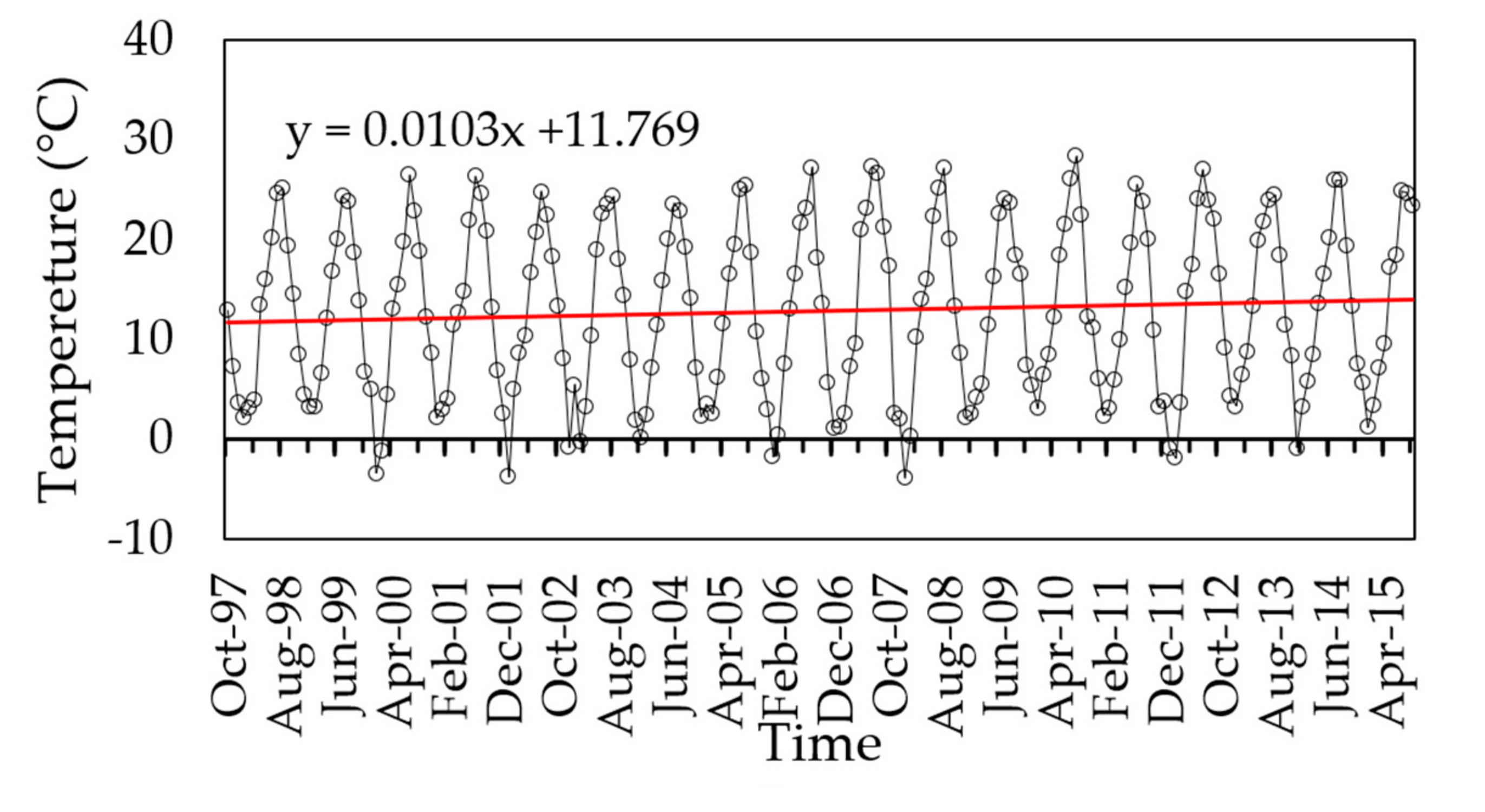
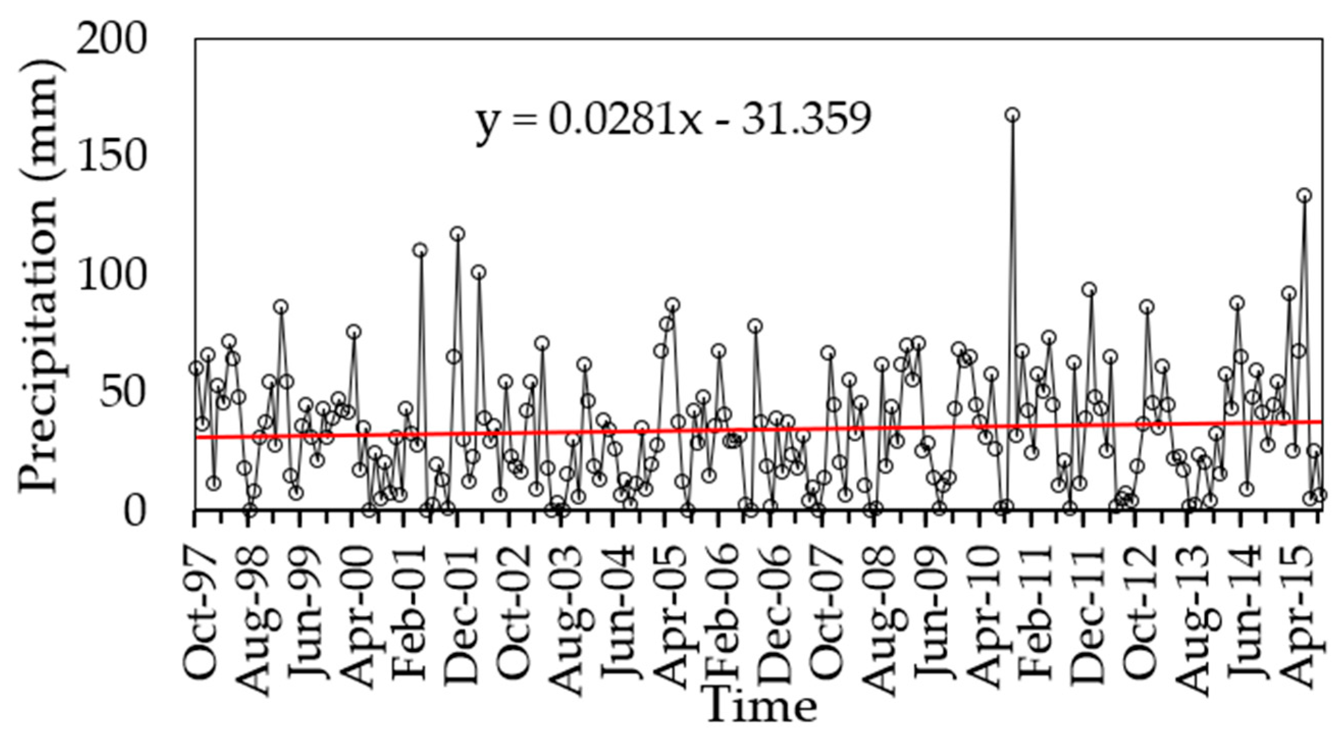
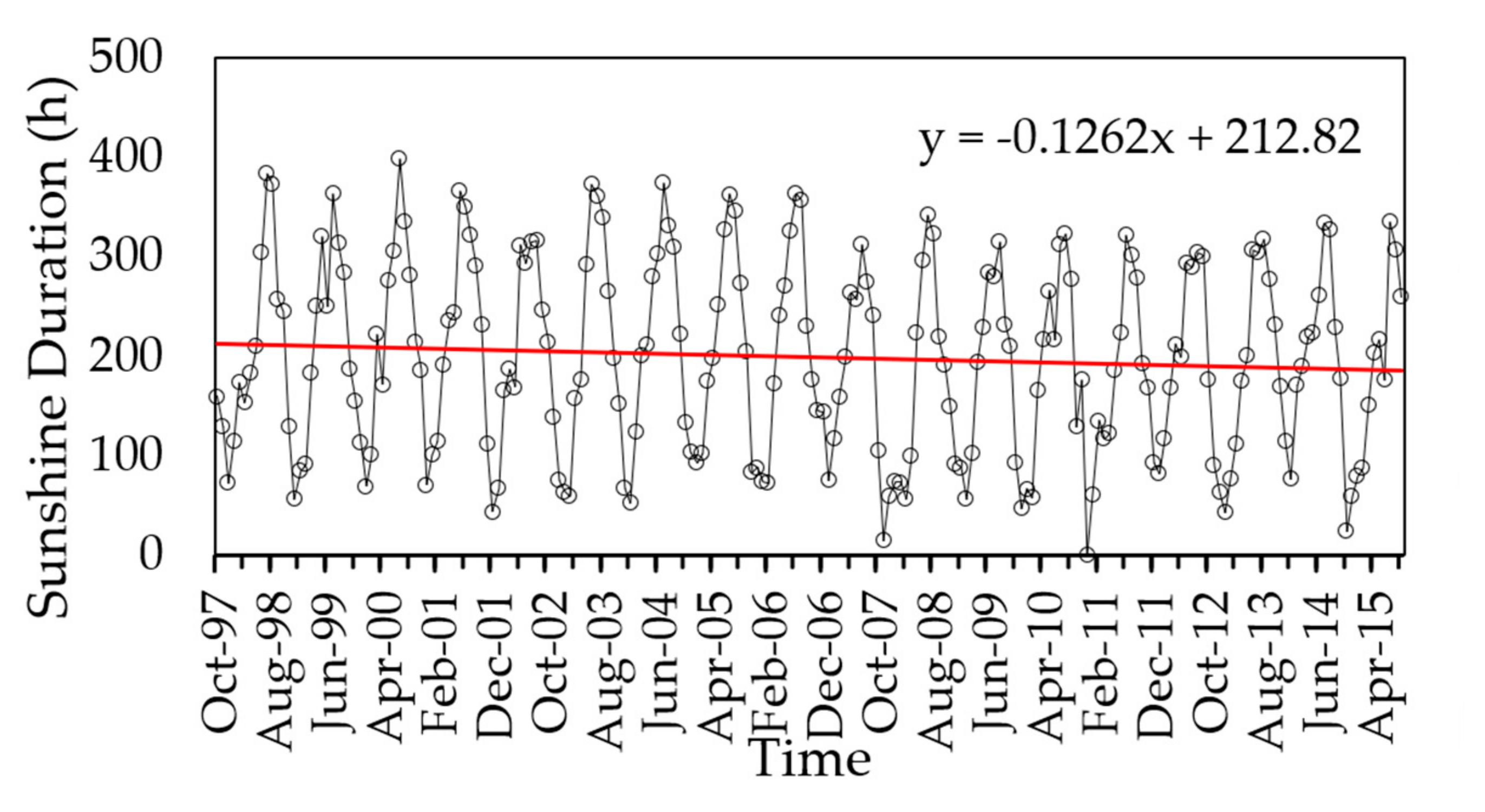
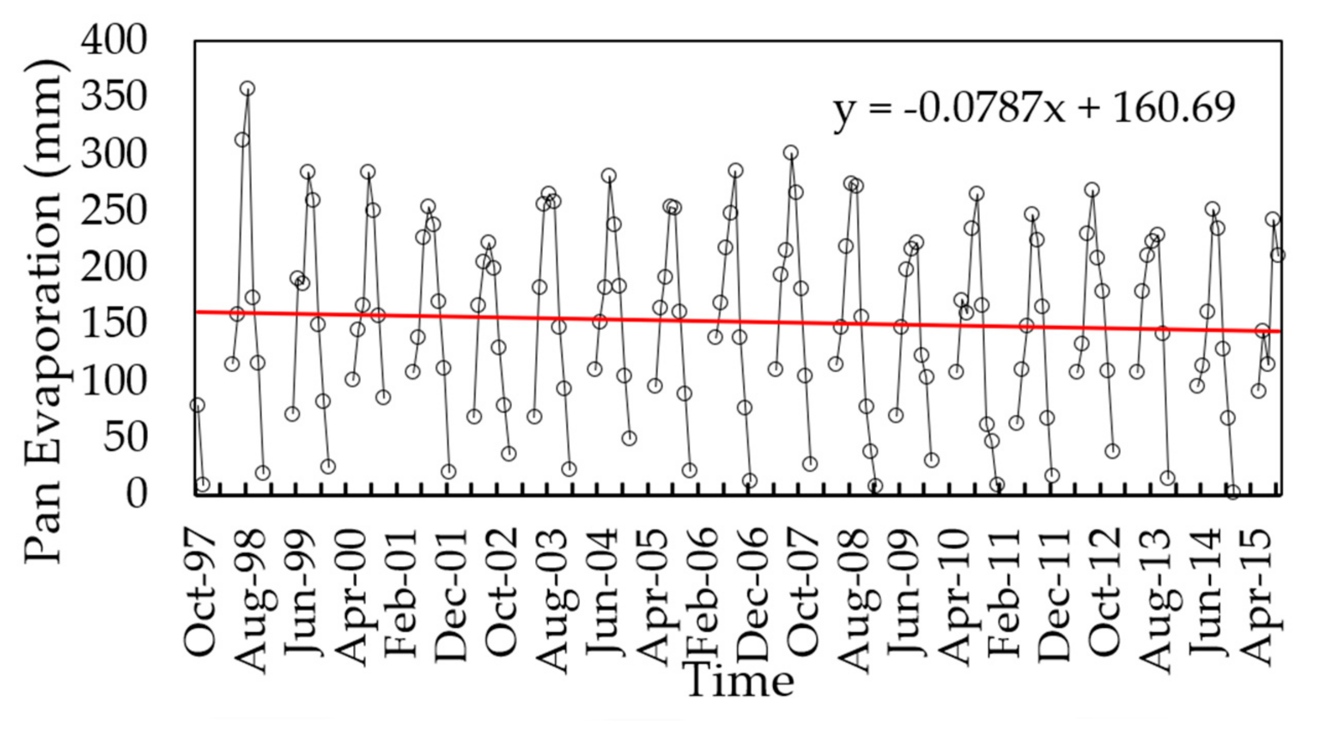
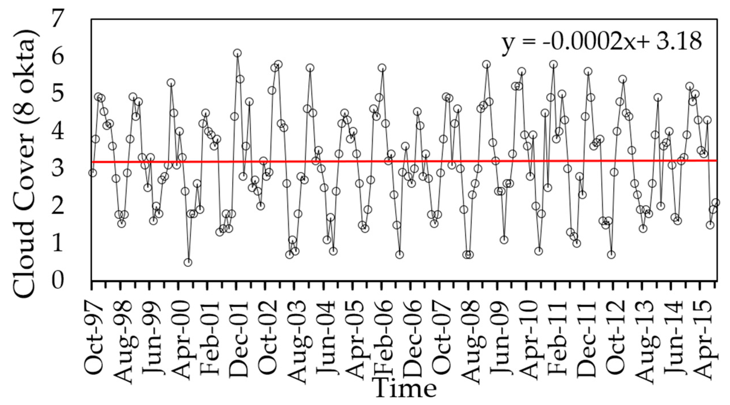
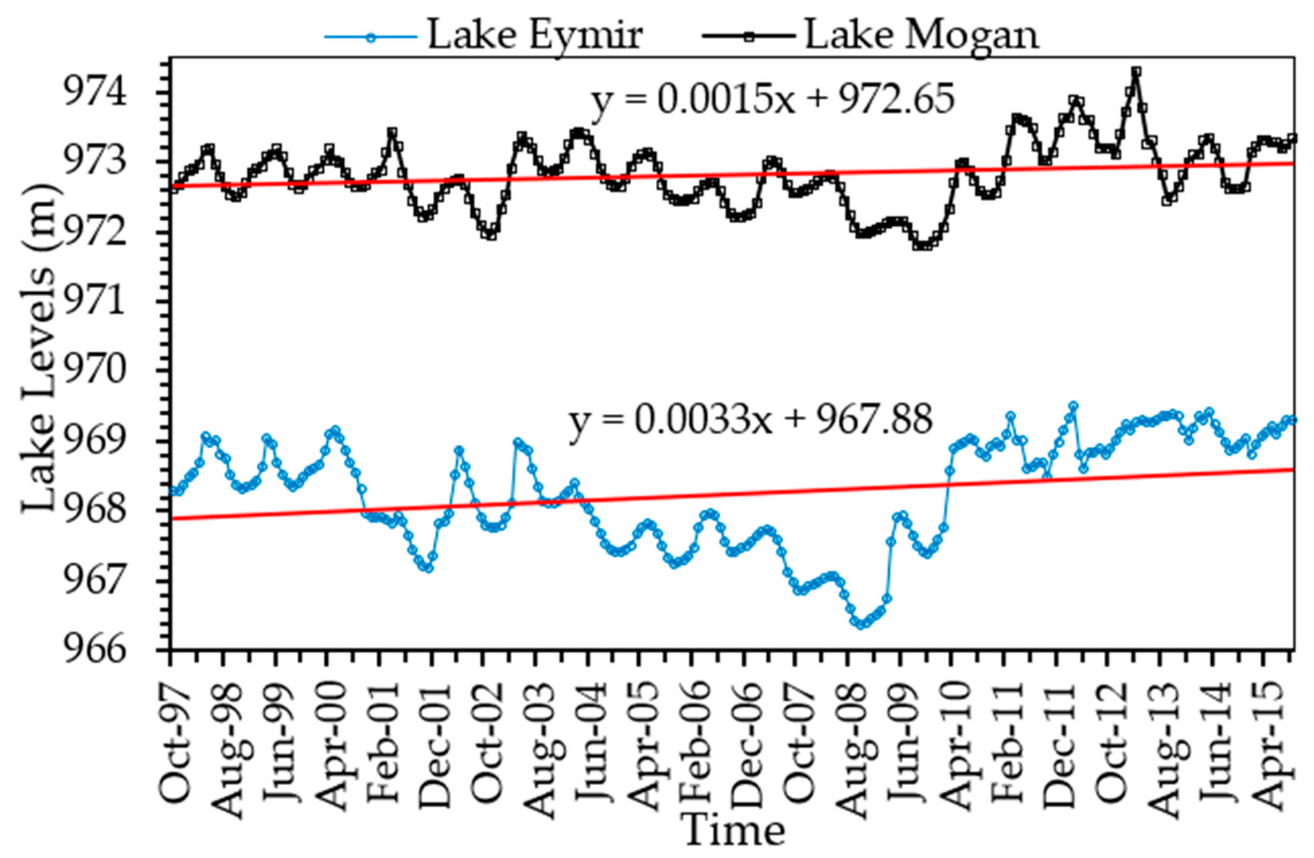
In the LT method, the regression equation is obtained by using the least-squares method according to the position and magnitude of the data in the time series. The β₁ value of the equation $\mathrm{Y}={\mathsf{\beta }}_0+{\mathsf{\beta }}_1\mathrm{X}$ indicates the slope of the equation. The t-statistics value of β₁ is calculated. Then the calculated t value is compared with the two-way critical value of the distribution of “t” at the selected confidence level. The “t” distribution is a special form of “Z” distribution and developed for small sample sizes. t critical values at ±5% confidence levels are ±1.971. Thus, if the calculated “t” value is greater than this value, there is a trend. Otherwise, it is concluded that the trend is not statistically significant. The results in Table 5 display decreasing trends for humidity and increasing trends for wind speed and lake levels at all confidence levels. Time series and linear trend analyses of all variables are given in Figure 3, Figure 4, Figure 5, Figure 6, Figure 7, Figure 8, Figure 9 and Figure 10.

In the ST method, the slope value “s” is calculated with the help of time series divided into equal parts Equation (8). This value is compared to the limit values (±CL) obtained by multiplying the calculated standard deviation by one-way normal distribution Z critical values (at specified confidence). The limit value is not a fixed number because the standard deviation of each variable is different Equation (12). The trend is not statistically significant if the limit value is greater than the slope value. If the limit value is smaller than the value of the slope, there is a trend and is in an ascending or descending direction depending on the sign. The results of the ST method are shown in Table 6 for various confidence levels. According to the ST results; temperature, precipitation, wind speed, cloud cover, and lake levels displayed increasing trends for all confidence levels. On the contrary, humidity, sunshine duration, and pan evaporation have shown decreasing trends at all confidence levels.

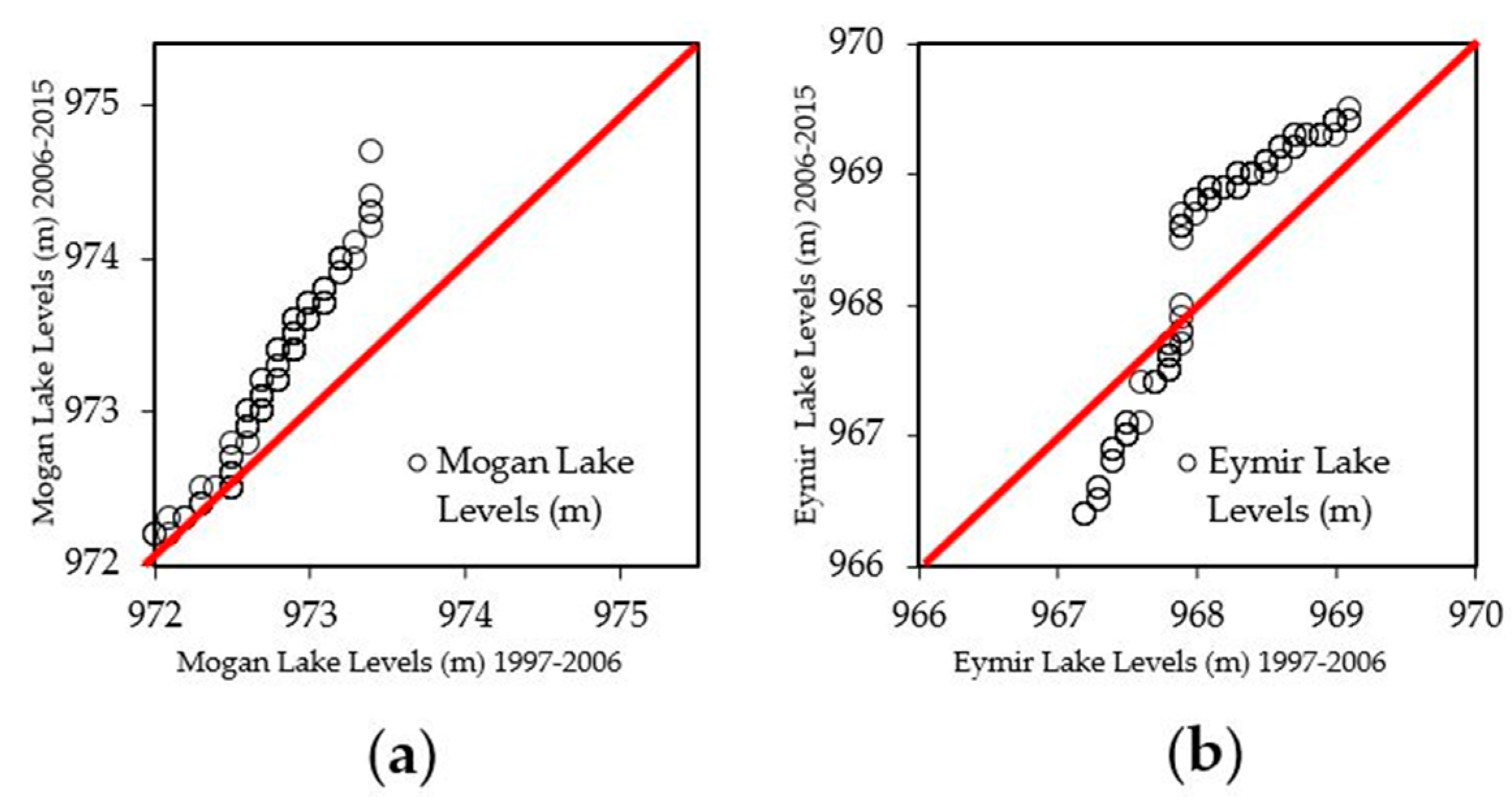
In the visualization of the ST results, data of Mogan lake levels in the second time series sorted according to the first time series fall into the upper triangular area, indicating an increasing trend (Figure 11a). In the case of Lake Eymir, while low values (967–968 m) of sorted data in the first time series versus second time series collected in the lower triangular area, indicating a decreasing trend, medium and high values (968–970 m) of sorted data collected in the upper triangular area, indicating an increasing trend (Figure 11b). The general trend region can be found by the average of first and second datasets. The averages of Lake Eymir’s first and second datasets are 968.14 m and 968.35 m, respectively. The averages of Lake Mogan’s first and second datasets are 972.78 m and 972.84 m, respectively. If the average of first and second data sets is equal, the average is located on the 1:1 (45°) straight line, indicating no trend. If the average of the first dataset is lower than the second dataset, the trend region is in the increasing area, according to the sorted data in the first data series. In the opposite situation, the trend region is in the decreasing part, according to the sorted data in the first data series. Thus, both lake levels’ general trends are in the increasing direction, according to the test results (Figure 11).

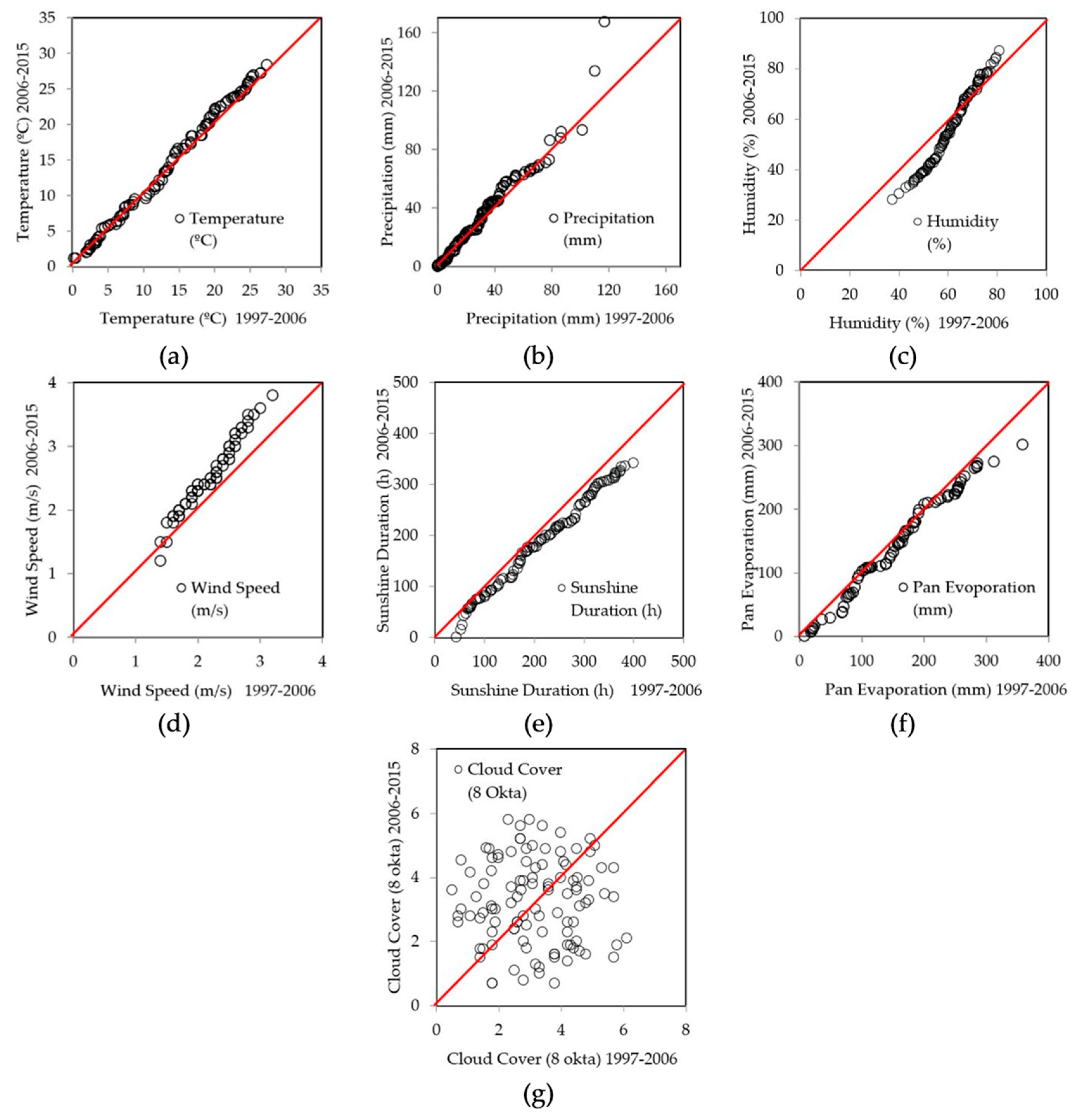
ST results of meteorological variables display the accumulation of precipitation, temperature, cloud cover, and wind speed data in the increasing trend region. However, the majority of humidity, sunshine duration, and pan evaporation data exist in the decreasing trend region (Figure 12), consistent with the statistical results given in Table 6.

4. Discussion

MATLAB programming language was used to perform the trend analyses. The overall evaluation and comparison of the trend test results for all four methods are summarized in Table 7. The results in Table 7 show that Eymir lake levels displayed statistically significant increasing trends in MK, MMK, LT, and ST methods at all confidence levels, except at the 99% confidence level in the MMK method. However, the Mogan lake levels showed statistically significant increasing trends in MK, LT, and ST methods, except at the 99% confidence level in the MK method. According to the MMK method, this trend is statistically insignificant for Mogan lake levels. The presence of strong autocorrelation in Mogan Lake levels has caused other methods to detect the trends significantly. The MMK method, which takes into account the effect of autocorrelation, differs from other methods in this aspect [13,24]. In view of meteorological variables, wind speed indicated significant increasing trends at all confidence levels in all four methods. On the contrary, significant decreasing trends in humidity were observed in all methods, except at the 99% confidence level for the MK and MMK tests. According to ST results; significant decreasing trends for the sunshine duration, pan evaporation, and humidity, and significant increasing trends at all confidence levels for temperature, precipitation, cloud cover, and wind speed were noticed.

The trend results implied that increasing precipitation and decreasing pan evaporation had resulted in increasing lake levels in both lakes. The results further demonstrated an inverse relationship between the trends of air temperature and pan evaporation, pointing out an apparent ‘Evaporation Paradox’ also observed in other locations. Decreases in pan evaporation over the last decades have been reported in many regions of the world associated with climate change [25,26,27,28]. The decrease in pan evaporation associated with the increasing air temperatures is called the “Pan Evaporation Paradox” [29]. Studies conducted in semi-arid regions point out that the combined contribution of cloud cover and relative humidity on pan evaporation is greater than that of temperature [30]. Thus, increased cloud cover offsets the increased pan evaporation because of temperature increase and relative humidity decrease. Our study shows that pan evaporation is a complex process for which all variables affecting pan evaporation should be taken into consideration in order to eliminate paradoxical observations, such as decreased pan evaporation with increased temperature as a result of global warming.

Comparison of trend analyses results from 96 monthly series (8 parameters × 4 methods × 3 confidence intervals) provided in Table 7 shows that significant trends (α = 10%, α = 5%, α = 1%) are detected in 7, 10, and 12 series using MMK, MK, and LT test, respectively. But 27 series show significant trends using the ST method, which indicate many significant trends (especially increasing trends for temperature, precipitation, cloud cover and decreasing trends for sunshine duration, and pan evaporation) that cannot be detected by LT, MK, or MMK test can be identified effectively by the ST method. Moreover, all significant trends that can be detected by the LT or MK test (10 series) can be effectively identified using the ST method. The test results using four methods indicates that ST method was very sensitive and superior to the LT, MK, and MMK test for the determination of the change in lake levels. This superior aspect of the ST method has been seen in many other studies in the literature [31,32,33,34]. In addition, all data ranges can be displayed graphically in the ST Cartesian coordinate system, so visual inspection and interpretation can also be made.

The increasing trends observed in lake levels over the period 1997–2015 were contrary to the predicted decreasing trends in lake levels using a lake-aquifer model [35], pointing out a significant difference over the precipitation and evaporation series used in the modeling work. The modeling work used precipitation and temperature series based on IPCC higher emission A2 and lower emission B1 scenarios, downloaded from the UNDP-supported research programme at Istanbul Technical University [36]. The results of these two scenarios predicted decreasing precipitation and increasing temperature for the City of Ankara over the period of 2004–2100. Consequently, the modeling results based on these series predicted decreasing lake levels over the period between 2004–2019, contrary to what has been observed over the same period. Therefore, the predictions of lake levels based on IPCC A2 and B1 emission scenarios cannot be considered accurate for the study area.

5. Conclusions

In the present study, the trends in water levels and meteorological variables affecting lake levels (average monthly pan evaporation, air temperature (°C), precipitation (mm), humidity (%), wind speed (m/s), sunshine duration (h), and cloud cover (8 okta)) over the Lakes Mogan and Eymir basin were analyzed using four methods: Mann-Kendall (MK), Modified Mann-Kendall (MMK), Sen Trend (ST), and Linear trend (LT) at 90%, 95%, and 99% confidence levels for the period 1997–2015.

The results show that three methods (MK, LT, ST) had an increasing trend in both lake levels at all confidence levels. While trend analyses of meteorological variables by Sen Test were significant at all tested variables and confidence levels, Mann-Kendall (MK) and Linear trend (LT) produced significant trends for only humidity and wind speed. When the results of MMK method are examined, it is seen that the trends are compatible with the MK and LT methods. Furthermore, Mogan lake levels, while showing an increasing tendency, is statistically insignificant in the MMK test due to the presence of autocorrelation in time series.

The trend analyses of the Sen Test gave increasing trends for temperature, wind speed, cloud cover, and precipitation; and decreasing trends for humidity, sunshine duration, and pan evaporation. These results show that increasing precipitation and decreasing pan evaporation resulted in increasing lake levels. When the trend methods are compared, the ST method was found to be more effective than other methods in determining the trend; it also allowed graphical interpretations with grouped data. The results of MK and LT method are very similar and trend directions are compatible. The MMK method, on the other hand, has been used successfully to detect trends when autocorrelation existed in the time series. The results further demonstrated an inverse relationship between the trends of air temperature and pan evaporation, pointing out an apparent “Evaporation Paradox” also observed in many other regions in the world. However, increasing cloud cover offsets the increased pan evaporation due to temperature increase and relative humidity decrease. Thus, pan evaporation is a complex process for which all variables affecting pan evaporation should be taken into consideration in order to eliminate paradoxical observations. Trend analyses of water level variations in Lakes Mogan and Eymir and meteorological variables will help to manage both lakes and associated ecosystems. Understanding the variation of water levels and the potential drivers can provide insights into lake conservation and management. Sustaining water at a proper level in both lakes is important for lake ecosystems and associated wetlands. Under the pressure of uncontrollable climatic variables, effective measures for sustainable integrated water resources management should be applied to preserve ecological integrity and ensure the water release and storage capacity of both lakes.

References

- Wantzen, K.M.; Rothhaupt, K.-O.; Mörtl, M.; Cantonati, M.; László, G.-T.; Fischer, P. Ecological effects of water-level fluctuations in lakes: An urgent issue. Hydrobiologia 2008, 613, 1–4. [Google Scholar] [CrossRef] [Green Version]
- Williamson, C.E.; Saros, J.E.; Vincent, W.F.; Smold, J.P. Lakes and reservoirs as sentinels, integrators, and regulators of climate change. Limnol. Oceanogr. 2009, 54, 2273–2282. [Google Scholar] [CrossRef]
- Beklioğlu, M.; Bucak, T.; Coppens, J.; Bezirci, G.; Tavsanoğlu, Ü.N.; Cakıroğlu, A.İ.; Levi, E.E.; Erdoğan, S.; Filiz, N.; Özkan, K.; et al. Restoration of eutrophic lakes with fluctuating water levels: A 20-year monitoring study of two inter-connected lakes. Water 2017, 9, 127. [Google Scholar] [CrossRef] [Green Version]
- Waylen, P.; Annear, C.; Bunting, E. Interannual hydroclimatic variability of the Lake Mweru basin, Zambia. Water 2019, 11, 1801. [Google Scholar] [CrossRef] [Green Version]
- McBean, E.; Motiee, H. Assessment of impact of climate change on water resources: A long term analysis of the Great Lakes of North America. Hydrol. Earth Syst. Sci. 2008, 12, 239–255. [Google Scholar] [CrossRef] [Green Version]
- Yuan, Y.; Zeng, G.; Liang, J.; Huang, L.; Hua, S.; Li, F.; Zhu, Y.; Wu, H.; Liu, J.; He, X.; et al. Variation of water level in Dongting Lake over a 50-year period: Implications for the impacts of anthropogenic and climatic factors. J. Hydrol. 2015, 525, 450–456. [Google Scholar] [CrossRef]
- Leira, M.; Cantonati, M. Effects of water-level fluctuations on lakes: An annotated bibliography. Hydrobiologia 2008, 613, 171–184. [Google Scholar] [CrossRef]
- Yagbasan, O.; Yazicigil, H.; Demir, V. Impacts of climatic variables on water-level variations in two shallow Eastern Mediterranean lakes. Environ. Earth Sci. 2017, 76, 575. [Google Scholar] [CrossRef]
- Büyükyildiz, M.; Yilmaz, V. Investigation of Water Level Changes of Some Lakes in Turkey. e-J. New World Sci. Acad. 2011, 6, 1061–1073. (In Turkish) [Google Scholar]
- Hu, M.; Sayama, T.; TRY, S.; Takara, K.; Tanaka, K. Trend analysis of hydroclimatic variables in the Kamo River Basin, Japan. Water 2019, 11, 1782. [Google Scholar] [CrossRef] [Green Version]
- Hamed, K.H. Trend detection in hydrologic data: The Mann-Kendall trend test under the scaling hypothesis. J. Hydrol. 2008, 349, 350–363. [Google Scholar] [CrossRef]
- Yu, Y.S.; Zou, S.; Whittemore, D. Non-parametric trend analysis of water quality data of rivers in Kansas. J. Hydrol. 1993, 150, 61–80. [Google Scholar] [CrossRef]
- Yue, S.; Pilon, P.; Phinney, B.; Cavadias, G. The influence of autocorrelation on the ability to detect trend in hydrological series. Hydrol. Process. 2002, 16, 1807–1829. [Google Scholar] [CrossRef]
- Davidson, R.; MacKinnon, J.G. Econometric Theory and Methods; Oxford University Press: New York, NY, USA, 2003; p. 768. [Google Scholar]
- Karabulut, M.; Cosun, F. Precipitation trend analyses in Kahramanmaraş. Coğrafi Bilimler Dergisi. 2009, 7, 65–83. (In Turkish) [Google Scholar]
- Ulke Keskin, A.; Beden, N.; Demir, V. Analysis of annual, seasonal and monthly trends of climatic data: A case study of Samsun. Nat. Sci. 2018, 13, 51–70. [Google Scholar] [CrossRef]
- Demir, V.; Zeybekoglu, U.; Beden, N.; Ulke Keskin, A. Homogeneity and trend analysis of long term temperatures in the Middle Black Sea Region. In Proceedings of the 13th International Congress on Advances in Civil Engineering, Izmir, Turkey, 12–14 September 2018; pp. 1–8. [Google Scholar]
- Mann, H.B. Non-parametric tests against trend. Econometrica 1945, 13, 245–259. [Google Scholar] [CrossRef]
- Kendall, M.G. Rank Correlation Methods; Charles Griffin Publishing: London, UK, 1975; p. 160. [Google Scholar]
- Helsel, D.R.; Hirsch, R.M. Statistical Methods in Water Resources. In Techniques of Water-Resources Investigations of the United States Geological Survey, Book 4, Hydrologic Analysis and Interpretation; Elsevier Publishers: Amsterdam, The Netherlands, 1992; p. 503. [Google Scholar]
- Sen, Z. Innovative trend analysis methodology. J. Hydrol. Eng. 2012, 17, 1042–1046. [Google Scholar] [CrossRef]
- Sen, Z. Trend identification simulation and application. J. Hydrol. Eng. 2014, 19, 635–642. [Google Scholar] [CrossRef]
- Sen, Z. Innovative trend significance test and applications. Theor. Appl. Climatol. 2017, 127, 939–947. [Google Scholar] [CrossRef]
- Hamed, K.H.; Ramachandra, A.R. A modified Mann-Kendall trend test for autocorrelated data. J. Hydrol. 1998, 204, 182–196. [Google Scholar] [CrossRef]
- Peterson, T.C.; Golubev, V.S.; Groisman, P.Y. Evaporation losing its strength. Nature 1995, 377, 687–688. [Google Scholar] [CrossRef]
- Thomas, A. Spatial and temporal characteristics of potential evapotranspiration trends over China. Int. J. Climatol. 2000, 20, 381–396. [Google Scholar] [CrossRef]
- Roderick, M.L.; Farquhar, G.D. The cause of decreased pan evaporation over the past 50 years. Science 2002, 298, 1410–1411. [Google Scholar] [PubMed]
- Liu, B.H.; Xu, M.; Henderson, M.; Gong, W.G. A spatial analysis of pan evaporation trends in China, 1955–2000. J. Geophys. Res. 2004, 109, D15102. [Google Scholar] [CrossRef] [Green Version]
- Brutsaert, W.; Parlange, M.B. Hydrologic cycle explains the evaporation paradox. Nature 1998, 396, 30. [Google Scholar] [CrossRef]
- Zhang, Q.; Wang, W.; Wang, S.; Zhang, L. Increasing trend of pan evaporation over the semiarid Loess Plateau under a warming climate. J. Appl. Meteorol. Climatol. 2016, 55, 2007–2020. [Google Scholar] [CrossRef]
- Güçlü, Y.S.; Dabanlı, I.; Şişman, E.; Şen, Z. Air quality (AQ) identification by innovative trend diagram and AQ index combinations in Istanbul megacity. Atmos. Pollut. Res. 2019, 10, 88–96. [Google Scholar] [CrossRef]
- Chandole, V.; Joshi, G.S.; Rana, S.C. Spatio-temporal trend detection of hydro-meteorological parameters for climate change assessment in Lower Tapi river basin of Gujarat state, India. J. Atmos. Sol. Terr. Phys. 2019, 195, 105130. [Google Scholar] [CrossRef]
- Wang, Y.; Xu, Y.; Tabari, H.; Wang, J.; Wang, Q.; Song, S.; Hu, Z. Innovative trend analysis of annual and seasonal rainfall in the Yangtze River Delta, eastern China. Atmos. Res. 2020, 231, 104673. [Google Scholar] [CrossRef]
- Zhou, Z.; Wang, L.; Lin, A.; Zhang, M.; Niu, Z. Innovative trend analysis of solar radiation in China during 1962–2015. Renew. Energy 2018, 119, 675–689. [Google Scholar] [CrossRef]
- Yagbasan, O.; Yazicigil, H. Assessing the impact of climate change on Mogan and Eymir Lakes’ levels in Central Turkey. Environ. Earth Sci. 2012, 66, 83–96. [Google Scholar] [CrossRef]
- Dalfes, H.N.; Karaca, M.; Sen, O.L. Climate change scenarios for Turkey. In Climate Change & Turkey-Impacts, Sectoral Analyses, Socio-Economic Dimensions; Çağlar, G., Ed.; United Nations Development Programme Turkey Office: Istanbul, Turkey, 2017. [Google Scholar]
Figure 1.
(a) Location of the study area. (b) Digital elevation map of the study area and location of the monitoring stations.
Figure 2.
Decreasing and increasing trends versus trend-free time series [16].
Figure 3.
Time series and linear trend analyses of temperature data between 1997 and 2015.
Figure 4.
Time series and linear trend analyses of precipitation data between 1997 and 2015.
Figure 5.
Time series and linear trend analyses of humidity data between 1997 and 2015.
Figure 6.
Time series and linear trend analyses of wind speed data between 1997 and 2015.
Figure 7.
Time series and linear trend analyses of sunshine duration data between 1997 and 2015.
Figure 8.
Time series and linear trend analyses of pan evaporation data between 1997 and 2015.
Figure 9.
Time series and linear trend analyses of cloud cover data between 1997 and 2015.
Figure 10.
Time series and linear trend analyses of lake levels between 1997 and 2015.
Figure 11.
ST graphics of lake levels: (a) Mogan Lake, (b) Eymir Lake.
Figure 12.
ST graphs of meteorological variables: (a) Temperature, (b) Precipitation, (c) Humidity, (d) Wind speed, (e) Sunshine duration, (f) Pan evaporation, (g) Cloud cover.