Can Soil Hydraulic Parameters be Estimated from the Stable Isotope Composition of Pore Water from a Single Soil Profile?

Abstract

Modeling water and solute transport in the vadose zone for groundwater resource management requires an accurate determination of soil hydraulic parameters. Estimating these parameters by inverse modeling using in situ observations is very common. However, little attention has been given to the potential of pore water isotope information to parameterize soil water transport models. By conducting a Morris and Sobol sensitivity analysis, we highlight the interest of combining water content and pore water isotope composition data in a multi-objective calibration approach to constrain soil hydraulic property parameterization. We then investigate the effect of the sampling frequency of the observed data used for model calibration on a synthetic case. When modeling is employed in order to estimate the annual groundwater recharge of a sandy aquifer, it is possible to calibrate the model without continuous monitoring data, using only water content and pore water isotopic composition profiles from a single sampling time. However, even if not continuous, multi-temporal data improve model calibration, especially pore water isotope data. The proposed calibration method was validated with field data. For groundwater recharge estimate studies, these results imply a significant reduction in the time and effort required, by avoiding long-term monitoring, since only one sampling campaign is needed to extract soil samples.

1. Introduction

Understanding water and solute movement in the vadose zone is fundamental to many environmental and natural resource issues. This includes the protection of groundwater, which is the main source of drinking water in many regions of the world [1,2,3], in terms of both quantity and quality. Numerical physically-based models are widely used to explore and predict water flow and solute transport in the vadose zone. The governing flow and transport equations are well-established, and a large number of analytical or numerical solutions have been published over the last four decades [4]. However, a number of numerical and conceptual difficulties remain to be solved, especially for field-scale processes subject to natural boundary conditions. This is typically the case for the estimation of soil hydraulic parameters, because of the pronounced spatial heterogeneity of the vadose zone [5].

Some of these parameters can be measured directly for soil samples in the laboratory. However, measured laboratory-scale properties have little relevance to describing field-scale water flow and transport processes under natural conditions [6,7]. This is due to spatial variability at the field scale which is not captured by limited sampling volumes, and to specific boundary conditions in the laboratory that differ from real-world conditions [8,9,10]. The inverse modeling approach is an established method that fits model simulations to observed data and results in effective parametrization, which lumps the subscale heterogeneity of the system and describes its behavior at the targeted scale [11]. A key question regarding the inverse modeling approach is whether the measurements are accurate enough and contain enough information to estimate the effective soil hydraulic parameters with the required accuracy.

The majority of field-scale inverse modeling studies have only used information on the water content (e.g., [12,13]). However, in situ observations of water content do not necessarily provide sufficient information to accurately parameterize field-scale soil hydraulic properties [14]. Combining different types of observed variables to calibrate water flow and transport models (e.g., water content and matric potential [15]; bromide concentration and water content [16]; water content and oxygen isotope composition [17]; water content and hydrogen isotope composition [18]; and water content, oxygen isotope composition, and matric potential [10]) has been found to improve parameterization.

In particular, water stable isotope (deuterium (²H) and oxygen-18 (¹⁸O)) profiles have been shown to provide valuable insights into hydrological processes in the vadose zone since several hydrological processes, such as infiltration [19], evaporation [20], and root water uptake [21], control the shape of the pore water-stable isotope profiles. The fact that stable isotopes are part of the water molecule, and are therefore extracted (without fractionation [22]) via root water uptake, is particularly helpful for constraining transpiration, which would not be possible with an artificial tracer. [18] demonstrated that water-stable isotope profiles, in combination with soil moisture time series, allow soil models to be calibrated and time-varying site-specific transit time distributions in the vadose zone to be derived.

To date, water content and pore water isotope composition profiles from a single sampling time have not been rigorously tested for their potential to calibrate soil hydraulic properties in the vadose zone in a humid climate. If possible, such an approach would reduce the time and effort required for long-term soil water content measurements, since only one sampling campaign would be necessary to obtain the soil samples required. The main objective of this study is to determine whether the inclusion of pore water isotope data allows a realistic parameterization of soil water transport models without the need for continuous monitoring data.

The METIS code [23], a vadose zone unsaturated/saturated transport model including isotope transport and isotopic fractionation due to evaporation, was used in this study to simulate soil water content and δ²H isotope data. A sensitivity analysis based on the methods of Morris [24] and Sobol [25] was performed to understand the interactions between soil hydraulic parameters and their impacts on modeled water content and isotope profiles and groundwater recharge calculation, and to highlight the interest of combining different observation types in model calibration. A synthetic case permitted insight into and a discussion of the performances of the calibration methods proposed here, compared with a calibration carried out using continuous monitoring data. Finally, the proposed calibration method was tested on field data. Using soil moisture and isotope profiles from a unique field campaign in a multi-objective approach to optimize model parameterization, a best set of soil hydraulic parameters was determined for two sites in southern Quebec, Canada. The accuracy of the parameterization for each site was assessed based on its ability to reproduce soil moisture and isotope profiles measured during a second campaign, one year later.

2. Materials and Methods

2.1. Site Description and Data Availability

The two sampling sites (SLA and SLB) were located in the Saint-Lawrence Lowlands, 60 km southwest of Montreal, in the Vaudreuil-Soulanges area (eastern Quebec, Canada). The study area has a humid climate with short, hot, and humid summers; cold and snowy winters; and rainy springs and autumns. The average annual precipitation in this area is 960 mm [26], with the average monthly temperature ranging from −11 to 23 °C [26]. The sites were located in a flat area in the southern part of Saint-Lazare (45°23′5.388″ N/74°11′50.316″ W), in the medium sands of the Saint-Lazare glacio-fluvial complex, which is a locally unconfined aquifer. The site SLA is located in grasslands 55 m from the site SLB, which is located in a pine forest. Further site characteristics are presented in

Table 1. Characteristics of the two study sites.

		SLA	SLB
Location		45°23′5.388″ N/74°11′50.316″ W	45°23′5.390″ N/74°11′50.320″ W
Elevation (m)		104	104
Geology		Cambrian formation	Cambrian formation
Soil depth (cm)	Horizon 1	0–20	0–30
	Horizon 2	20–200	30–200
Soil texture *	Horizon 1	Medium sand	Medium sand
	Horizon 2	Medium sand	Medium sand
Organic matter (%) **	Horizon 1	3	6
	Horizon 2	0	<1
Soil particle density (g cm−3)	Horizon 1	2.1	1.2
	Horizon 2	2.4	2.4
Land use		Grassland	Pine forest
Maximum rooting depth (cm)		10	20

* Texture classification system of Folk and Ward (1957) [29]. ** Large uncertainty exists.

.

At both sites, the unsaturated zone was sampled on 23 November 2017 and 9 November 2018. Approximately 800 g of soil samples was taken with a spatula, with a spacing of 5 cm between the soil surface to a 30 cm depth, and then 10 cm down to a 200 cm depth. Soil samples were stored in air-tight glass jars until water-stable isotope measurements were performed by laser spectrometry (TIWA-DLP-EP) at GEOTOP-UQAM using the direct vapor equilibration method [27]. The gravimetric water content and solid phase density were measured in the laboratory for the bulk samples.

Daily weather data (minimum and maximum temperature, precipitation, and relative humidity) with a 32 km grid spacing were obtained from the North American Regional Reanalysis (NARR) [28]. Monthly precipitation isotope composition values were measured at Mont-Saint Bruno (75 km from the study site) from January 2015 to November 2018.

A piezometer was installed in 2015 between the SLA and SLB sites. During the studied period (1 January 2016 to 31 December 2018), the water table level fluctuated between a 6.5 m and 4.5 m depth.

2.2. Model Description

2.2.1. Water Flow

Transient water flow within the unsaturated soil profile was simulated by numerically solving the Richards equation using the finite-element code, METIS (1D), developed by the Geosciences Department of MINES ParisTech [23]:

$$\mathrm{div}({\mathrm{K}}_{\mathrm{s}}{ \mathrm{K}}_{\mathrm{r}}\mathrm{grad} \mathrm{H})=\left(\mathrm{F} \mathrm{C}\left(\mathrm{h}\right)\right)\frac{\partial \mathrm{H}}{\partial \mathrm{t}} ,$$

(1)

where K_s is the saturated hydraulic conductivity (L T⁻¹); K_r is the relative hydraulic conductivity (-); H is the hydraulic head (L); F is the porosity (L³ L⁻³); and C(h) is the specific retention capacity specified by S, the saturation ratio (L³ L⁻³), and h, the matric head (L):

$$\mathrm{C}\left(\mathrm{h}\right)=\frac{\partial \mathrm{S}}{\partial \mathrm{h}}$$

(2)

The behavior of the unsaturated medium depends on two essential characteristics of the material: the relative permeability curve and the suction curve. These relationships are determined by the residual and maximal saturation ratio (S_min (L³ L⁻³) and S_max (L³ L⁻³), respectively); three empirical parameters defining the shape of the retention curves: α (L⁻¹), n (−), and m (−) (with m = 1 − 1/n); and K_s, the saturated hydraulic conductivity (L T⁻¹), following the Mualem–van Genuchten (MvG) model [30,31]:

$${\mathrm{K}}_{\mathrm{r}}\left(\mathrm{h}\right)= \sqrt{\frac{\mathrm{S}\left(\mathrm{h}\right)-{\mathrm{S}}_{\min }}{{\mathrm{S}}_{\max }-{\mathrm{S}}_{\min }}} {\left[1-{\left(1-{\left(\sqrt{\frac{\mathrm{S}\left(\mathrm{h}\right)-{\mathrm{S}}_{\min }}{{\mathrm{S}}_{\max }-{\mathrm{S}}_{\min }}}\right)}^{\frac{1}{\mathrm{n}}}\right)}^{\mathrm{n}}\right]}^2,$$

(3)

$$\frac{\mathrm{S}\left(\mathrm{h}\right)-{\mathrm{S}}_{\min }}{{\mathrm{S}}_{\max }-{\mathrm{S}}_{\min }}=\frac{1}{{\left[1+{\left(\mathsf{\alpha }\left|\mathrm{h}\right|\right)}^{\mathrm{n}}\right]}^{\mathrm{m}}.}$$

(4)

In order to account for root water uptake, a sink term was defined according to [32]. The required matric potential that describes the minimal pressure head for the root water uptake should be calculated using the Kelvin equation [33]. However, for sandy soil or gravel, due to numerical constraints, one needs to use high values. Here, the matric potential was set to −1000 cm. Root water uptake was parameterized by the site-specific rooting depth (Table 1) and a uniform root distribution.

Potential evapotranspiration (PET) was estimated using the Hargreaves and Samani formula [34] as a function of extraterrestrial radiation and daily maximum and minimum air temperature. As evaporation changes the isotopic composition of the pore water remaining in the soil by fractionation, whereas transpiration does not [22], potential evaporation and potential transpiration must be considered separately in the model. PET is therefore split into potential evaporation and potential transpiration according to Beer’s law [35], which is a function of the leaf area index (LAI) and the canopy radiation extinction factor (set to 0.463, as per [36]).

Snow is typical during the winter season in the study area. Snow cover was modeled using the two-parameter semi-distributed Snow Accounting Routine model, CEMANEIGE [37]. Precipitation during periods with temperatures of less than 0 °C was assumed to take the form of snow, and did not immediately infiltrate the soil. Snow melt was then simulated by assuming it to be proportional to the air temperature above 0 °C, using a degree-day snow melting constant of 0.5 mm day⁻¹ °C⁻¹ and a cold content factor of 0.1. Groundwater recharge was calculated as downward water flux (L T⁻¹) at the bottom of the profile.

2.2.2. δ²H Transport

In the METIS code, ²H transport in soil is calculated according to the widely used advection–dispersion model, with dispersivity (λ (L)) as the only parameter [38]. The absolute value of δ (in parts per thousand Vienna Standard Mean Ocean Water (VSMOW)) is used to represent the isotopic concentration. Isotopic enrichment due to fractionation processes during evaporation was included in the model based on the formulation introduced by Gonfiantini (1986) [39] for isotope mass balance, as follows:

$${\mathsf{\delta }}_{\mathrm{s}}={\mathsf{\delta }}^{\ast }+\left({\mathsf{\delta }}_{\mathrm{p}}-{ \mathsf{\delta }}^{\ast }\right){\left(1-\mathrm{f}\right)}^{\mathrm{m}},$$

(5)

where δ_S is the isotopic signal of the soil water in the upper centimeter, f is the fraction of evaporated water, ${\mathsf{\delta }}_{\mathrm{p}}$ is the isotopic signal of the water at the previous time step, ${\mathsf{\delta }}^{\ast }$ is the limiting isotopic enrichment factor, and m is the enrichment slope, as described below. For more details, see [40].

δ* is a function of air humidity, a; the isotopic composition of ambient air, δ_A; and a total enrichment factor, ε [41]:

$${\mathsf{\delta }}^{\ast }=\frac{\mathrm{a} \times { \mathsf{\delta }}_{\mathrm{A}}+ \mathsf{\epsilon }}{\mathrm{a} - \frac{\mathsf{\epsilon }}{100}} .$$

(6)

δ_A is calculated based on the stable isotopic signal of precipitation, ${\mathsf{\delta }}_{\mathrm{rain}},$ and the isotope fractionation factor, ε+, according to [42]

$${\mathsf{\delta }}_{\mathrm{A}}=\frac{{\mathsf{\delta }}_{\mathrm{rain}}+{ \mathsf{\epsilon }}^{+}}{{\mathsf{\alpha }}^{+}} ,$$

(7)

with ${\alpha }^{+}$ being the equilibrium isotope fractionation factor defined by Horita and Wesolowski (1994) [43].

The temperature-dependent equilibrium isotope fractionation factor, ε⁺, is defined as

$${\mathsf{\epsilon }}^{+}=\left({\mathsf{\alpha }}^{+}-1\right) \times 1000.$$

(8)

The total fractionation factor, ε, is equal to the sum of the equilibrium isotope fractionation factor, ε⁺, determined above (Equation (8)), and the kinetic isotope fractionation factor, ε_K, defined by Gat (1995) [44]:

$${\mathsf{\epsilon }}_{\mathrm{k}}=\left(1-\mathrm{a}\right) \times { \mathrm{C}}_{\mathrm{k}},$$

(9)

where C_k is the kinetic fractionation constant equal to 12.5‰ for δ²H.

The enrichment slope m is given by

$$\mathrm{m}=\frac{\mathrm{a}- \frac{\mathsf{\epsilon }}{1000}}{1-\mathrm{a}+ \frac{{\mathsf{\epsilon }}_{\mathrm{k}}}{1000}} .$$

(10)

2.2.3. Initial and Boundary Conditions

For all study sites, the depth of the soil profiles was set to 600 cm and discretized into 601 nodes. The profiles were divided into two different horizons (horizon 1 and horizon 2) according to the field observations (Table 1).

The results of steady-state simulations of water content and a constant pore water isotope composition, representing the weighted average concentration in precipitation (−85‰ for δ²H, Figure S1, in the supplementary material), were used as site-specific initial conditions. The modeled period extended from 1 January 2016 to 31 December 2018. The effect of the initial conditions on the calibration can be neglected, as a spin-up period of almost 2 years (1 January 2016 to 23 November 2017) was simulated prior to calibration.

The upper boundary condition was defined by variable atmospheric conditions that govern the loss of water and deuterium by evaporation, and the input of water due to infiltration and the accompanying flux concentrations of deuterium. The bottom boundary condition was set to zero-potential to represent the average water table level observed in the field.

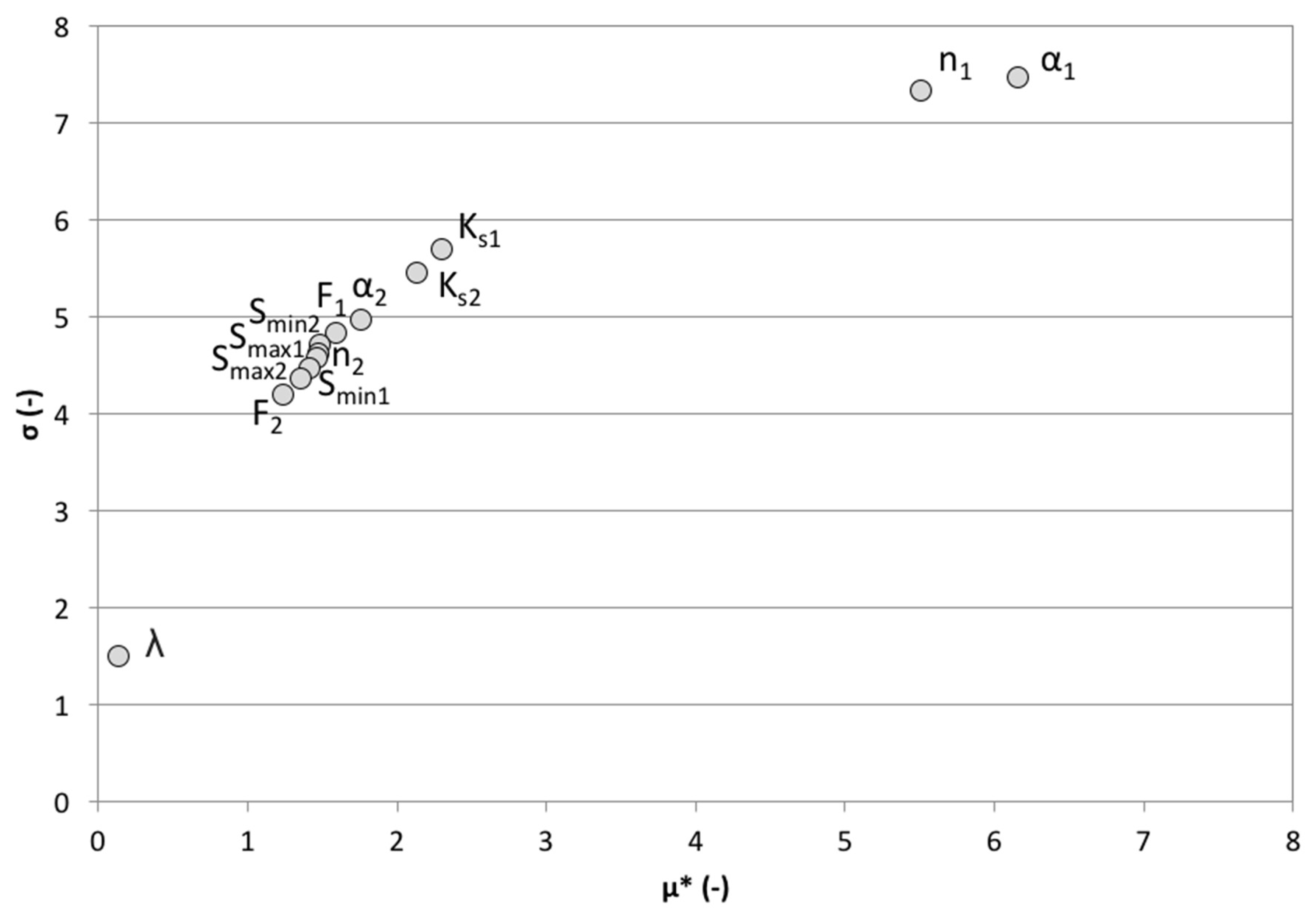
2.3. Sensitivity Analyses

Environmental optimization studies are often affected by the equifinality problem [45], whereby multiple sets of parameters can produce similar results. This problem is exacerbated with large numbers of parameters and when only limited information about their interactions and their effects on the output is available. In the METIS code, six parameters have to be optimized for each horizon of the soil profiles to simulate water flow in the unsaturated zone: S_min, S_max, α, n, and K_s, describing the water retention and hydraulic conductivity characteristics in accordance with the MvG model and F soil porosity. The dispersivity, λ, also has to be optimized to simulate δ²H value dispersion in soil. The same dispersivity value was assumed for both horizons [38].

Water and δ²H transport equations are known to be highly non-linear; however, little attention has been given to quantifying the influence of each parameter, individually and through interaction, on groundwater recharge estimates. To fill this gap, sensitivity analyses were performed in order to identify the most influential soil hydraulic parameters and their interactions, and to determine how these parameters affect groundwater recharge estimation. Additionally, in order to demonstrate if information contained in the isotope and water content profiles from a single sampling time are complementary in their abilities to optimize soil hydraulic parameters by inverse modeling, sensitivity analyses were performed to understand how soil hydraulic parameters affect the modeled water content and isotope profiles at a specific time.

Sensitivity analyses presented below were performed for a synthetic case. Simulated recharge, water content, and isotope profiles were obtained using the boundary conditions described above (Section 2.2.3) and the soil hydraulic parameters presented in

Table 2. Comparison of soil hydraulic parameters obtained using different types of data in the optimization procedure. The set of reference parameters is the “synthetic case”. To calibrate the model, the other cases rely on one water content profile at a single time (case 1); one water content profile and one pore water isotope composition profile at a same single time (case 2); monthly monitoring of the water content and pore water isotope composition at a 15 cm depth, plus one water content and one pore water isotope composition profile at a single time (case 3); and daily water content monitoring at 10, 20, 50, and 100 cm depths, plus one water content and pore water isotope composition profile at a single time (case 4).

		n	α	Ks	F	Smin	Smax	λ
		(-)	(m−1)	(m s−1)	(-)	(-)	(-)	(m)
Synthetic case	Horizon 1	2.00	5.00	1.00 × 10−3	0.40	0.02	0.60	0.01
	Horizon 2	3.00	10.00	1.00 × 10−4	0.35	0.05	0.55	0.01
Case 1	Horizon 1	1.78	4.97	2.33 × 10−3	0.32	0.12	0.54	0.01
	Horizon 2	2.37	21.36	8.63 × 10−3	0.23	0.09	0.29	0.01
Case 2	Horizon 1	1.31	8.91	2.94 × 10−3	0.37	0.05	0.51	0.01
	Horizon 2	2.12	27.48	7.61 × 10−3	0.37	0.08	0.60	0.01
Case 3	Horizon 1	1.46	10.49	2.69 × 10−4	0.39	0.01	0.50	0.01
	Horizon 2	2.37	23.80	1.25 × 10−4	0.20	0.04	0.54	0.01
Case 4	Horizon 1	1.46	10.49	2.69 × 10−4	0.39	0.01	0.50	0.01
	Horizon 2	2.37	23.80	1.25 × 10−4	0.20	0.04	0.54	0.01

, for a period of 3 years (1 January 2016 to 31 December 2018).

2.3.1. The Morris Method

In this study, the modified version of the Morris method proposed by [24] was used to investigate input soil hydraulic parameters to which groundwater recharge is most sensitive. The Morris method performs “One-At-a-Time” (OAT) analyses, whereby each parameter is varied one after another and the relative variation in model output (referred to as the Elementary Effect, E) is measured. Each parameter, X, is randomly selected in the input space, and the variation direction is also random. The repetition (r times) of OAT analyses allows the full input parameter space to be scanned. Along each trajectory, the so-called elementary effect of parameter X_j for the i-th repetition is defined as

$${\mathrm{E}}_{\mathrm{j}}^{\mathrm{i}}=\frac{\mathrm{Y}\left(\mathrm{X}+\Delta {\mathrm{e}}_{\mathrm{j}}\right)-\mathrm{Y}\left(\mathrm{X}\right)}{\Delta },$$

(11)

where Y is the model output with parameter set X, Δ is a value chosen in the range of {1/(p−1),..,1−1/p−1)} by the user, p is the number of discretization levels, and e_j is a vector of the canonical basis. [24] recommends that Δ equals p/2(p−1). For any X_j selected in the input space, X + Δe_j is always in the input space.

To assess the sensitivity of the input factors, two indices, σ and μ*, are computed as follows:

$${\mathsf{\mu }}_{\mathrm{j}}^{\ast }= \frac{1}{\mathrm{r}}{{\displaystyle \sum }}_{\mathrm{i}=1}^{\mathrm{r}}\left|{\mathrm{E}}_{\mathrm{j}}^{\mathrm{i}}\right|,$$

(12)

$${\mathsf{\sigma }}_{\mathrm{j}}= \sqrt{\frac{1}{\mathrm{r}}{{\displaystyle \sum }}_{\mathrm{i}=1}^{\mathrm{r}}{\left({\mathrm{E}}_{\mathrm{j}}^{\mathrm{i}}-\frac{1}{\mathrm{r}}{{\displaystyle \sum }}_{\mathrm{i}=1}^{\mathrm{r}}{\mathrm{E}}_{\mathrm{j}}^{\mathrm{i}}\right)}^2}.$$

(13)

µ_j^* estimates the overall impact of the parameter X_j on the model output, and σ_j measures the non-linear and/or interaction effects with other parameters.

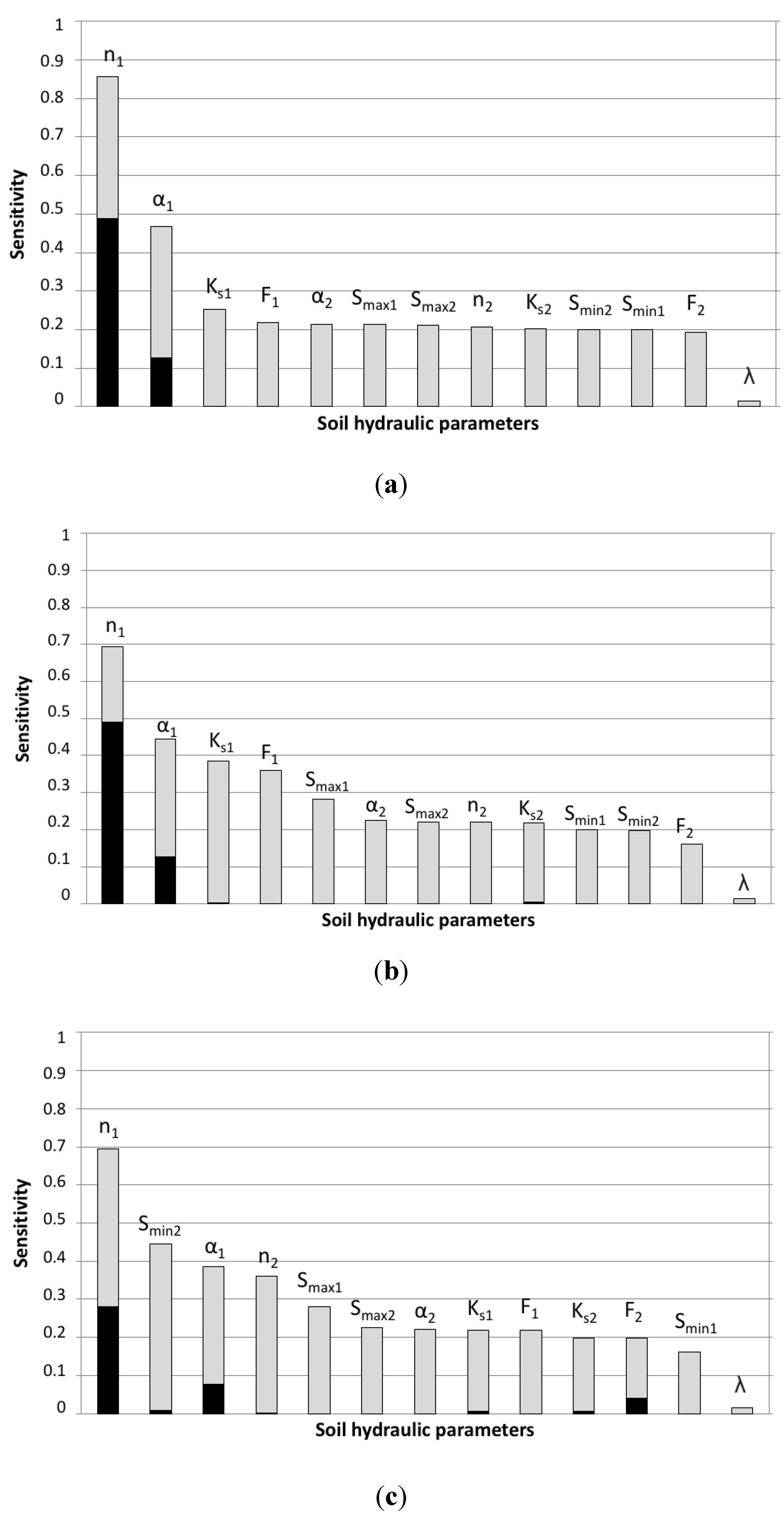
2.3.2. The Sobol Method

A modified version of the Sobol sensitivity analysis [46] was performed for the most influent input soil hydraulic parameters identified by the Morris method in order to quantify the amount of variance that each parameter contributes to the unconditional variance of the model output. These amounts are represented by Sobol’s sensitivity indices (SIs). The SIs give quantitative information on the variance associated with a single parameter or related to interactions of multiple parameters. For a more complete explanation of the Sobol method, please refer to Sobol (2001) [25]. Sobol’s sensitivity indices are expressed as follows:

$$\text{First-order} \mathrm{indices}:{\mathrm{S}}_{1,\mathrm{i}}= \frac{{\mathrm{V}}_{\mathrm{i}}}{\mathrm{V}} ,$$

(14)

$$\text{Second-order} \mathrm{indices}:{\mathrm{S}}_{\mathrm{i},\mathrm{j}}= \frac{{\mathrm{V}}_{\mathrm{ij}}}{\mathrm{V}} ,$$

(15)

$$\mathrm{Total} \mathrm{indices}:{\mathrm{S}}_{\mathrm{Ti}}={ \mathrm{S}}_{1,\mathrm{i}}+ {{\displaystyle \sum }}_{\mathrm{j}\ne \mathrm{i}}{\mathrm{S}}_{\mathrm{ij}} ,$$

(16)

where V_i is the variance associated with the ith parameter and V is the total variance.

The first order index, S_1,j, represents the individual variance contribution of the parameter X_i to the total unconditional variance, also referred to as the “main effect”. The second order index, S_i,j, explains the interaction effect between parameters X_i and X_j. The overall impact of parameter X_i, including the main effect and all its interactions with other parameters, is given by the total index S_Ti. If the sum of all first-order indices is less than 1, the model is non-additive.

Sobol sensitivity analysis was performed for groundwater recharge, which is ultimately the targeted output variable, as well as for soil water content and pore water isotope profiles simulated at a single sampling time, in order to investigate the benefit of combining soil water content and tracer data in the optimization procedure.

2.3.3. Implementation of the Sensitivity Analyses

The Python programming language and the Sensitivity Analysis Library (SALib) [47] in particular were used to conduct the sensitivity analyses. Sensitivity indices are calculated for scalar outputs obtained from objective functions. Here, the modified Kling–Gupta efficiency (KGE) index, as defined by [48], was used as the objective function (Equation (17)). This dimensionless index compares simulated and observed data with regards to their correlation (r), the ratio of their mean values (bias ratio, β), and the ratio of their coefficient of variation (variability ratio, γ) as follows:

KGE = 1 − [(1 − r )² +(1 − β)² +(1 − γ) ²]^0.5.

(17)

Values of the objective function are stored in a one-dimensional array for the subsequent computation of the sensitivity indices. If the METIS code needs to reduce the computation step to less than one second, it is considered to be non-convergent; the script then terminates the simulation and attributes a large negative value to the objective function (−100). The same negative value is attributed when the duration of the modeled groundwater recharge is shorter than one year, which indicates that the run was unsuccessful.

2.4. Model Calibration

2.4.1. Data Types

This study focuses on the type of data used for model calibration and the implications when using the model to predict groundwater recharge. Four data types have been tested here using different approaches:

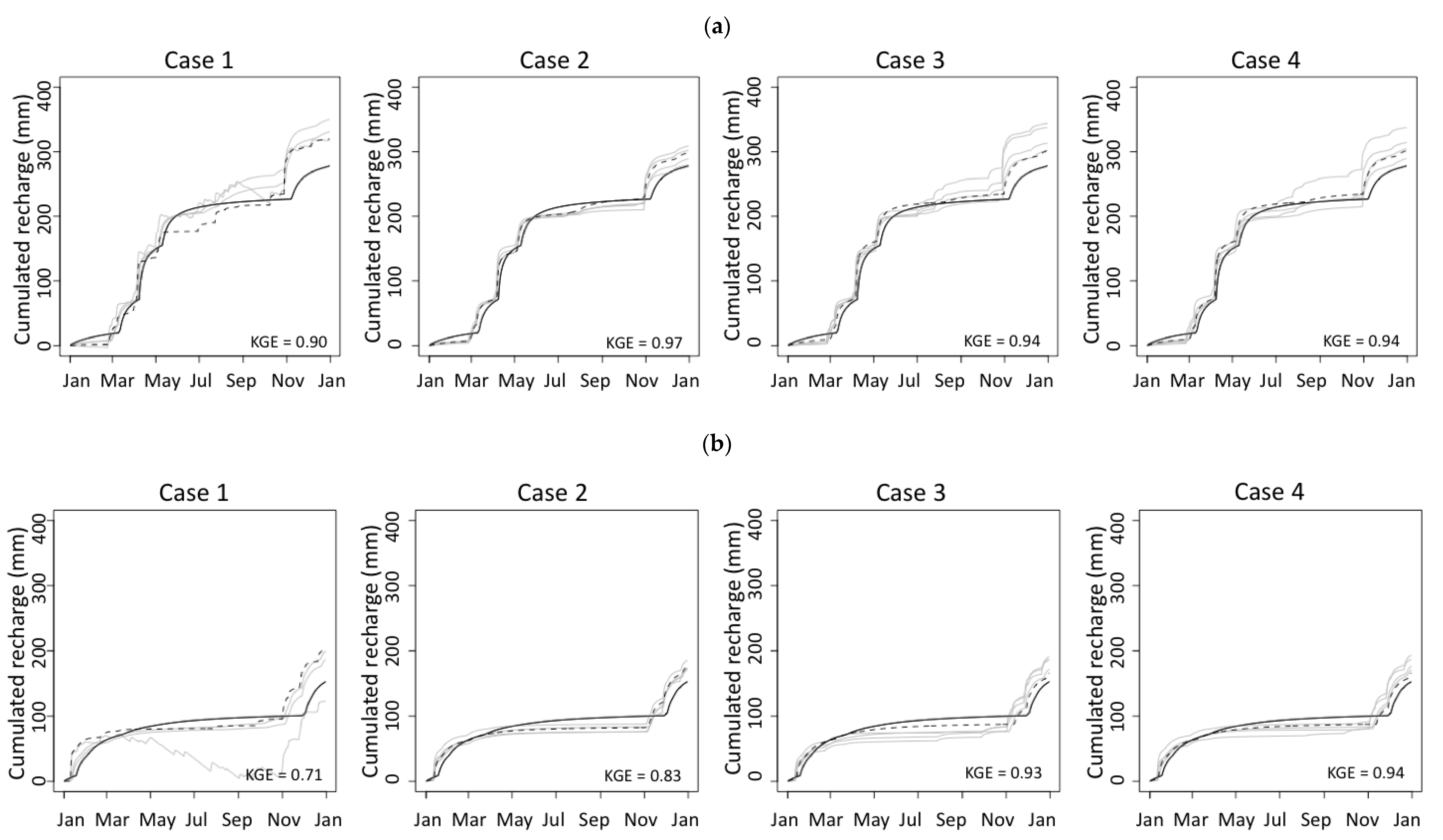
• The one-profile approach uses a single depth profile of the water content at a single sampling time (case 1) or one depth profile of both the water content and pore water isotope composition at a given time (case 2) to calibrate the soil hydraulic parameters. This approach does not require continuous monitoring data as it is only based on profiles at a given sampling time. Such a method facilitates model calibration by avoiding the time, cost, and effort associated with long-term soil water content measurements, since only one sampling campaign is needed to obtain the soil samples;
• The monthly approach (case 3) uses the monthly water content and pore water isotope composition at a 15 cm depth, plus one depth profile of both the water content and pore water isotope composition at a given time (as in case 2), to calibrate the soil hydraulic parameters;
• The daily approach (case 4) uses daily monitoring of the water content at four different depths (10, 20, 50, and 100 cm), and one depth profile of both the water content and pore water isotope composition at a single time to calibrate the soil hydraulic parameters. [18] used this approach.

As neither monthly water content or pore water isotope composition monitoring data from a 15 cm depth nor daily water content monitoring data from 10, 20, 50, and 100 cm depths were available for our study sites, we used the synthetic case to discuss the performances of the optimization procedures. Simulated water content and isotope profiles were obtained using the boundary conditions described above (Section 2.2.3) and the soil hydraulic parameters presented in Table 2, for a period of 3 years (1 January 2016 to 31 December 2108). These simulated data were subsampled with a spacing of 5 cm between the soil surface to a 30 cm depth, and then 10 cm down to a 200 cm depth. These subsampled data were used in place of observed data. The realism of the parameterization obtained with the different calibration approaches was assessed based on their abilities to reproduce observed groundwater recharge, both in terms of quantity and dynamics.

2.4.2. Multi-Objective Optimization Procedure

An optimization procedure was developed to calibrate soil hydraulic parameters of a two-layer model (i.e., α₁, n₁, S_min1, S_max1, K_s1, F₁, α₂, n₂, S_min2, S_max2, Ks₂, F₂, and λ) based on the difference between the measured and simulated soil moisture and pore water isotope composition. The Latin Hypercube Sampling (LHS) method [49] was used to sample soil hydraulic parameters in the 13-dimension parameter space. The range (min, max) for each parameter was chosen according to expert knowledge [21] and 5000 values were randomly chosen from within this range (Table 2). The LHS method ensures that parameter ranges are equally sampled and fully explored. Each computation is initiated with a different set of soil hydraulic parameters, and soil moisture and pore water isotope data are computed with these different parameter combinations. For each simulation, three KGE were calculated: soil moisture (KGE_θ), isotope data (KGE_c), and the average of both (KGE_tot). Sequential and simultaneous multi-objective approaches have already been tested elsewhere [10,18] and the simultaneous multi-objective approach was shown to be a time-efficient calibration procedure, resulting in a good representation of water flow and isotope transport. The set of soil hydraulic parameters leading to the best KGE_tot was retained.

3. Results and Discussion

3.1. Sensitivity Analyses

Morris sensitivity analysis method results produced for groundwater recharge (obtained from the synthetic case) are reported in Figure 1. To interpret the results by simultaneously taking into account both sensitivity measures, we used representation in the (μ*-σ) plane, which allows soil hydraulic parameters to be classified into three types: parameters having negligible effects, with small μ* and σ; parameters having non-linear effects and/or interactions with other parameters, with large μ* and σ; and parameters having linear and additive effects, with large μ* and small σ. Parameters α₁ and n₁ present particularly strong non-linear effects and/or interactions with other parameters. All factors with a high μ* value also have a high σ value, indicating that none of the parameters have a purely linear effect. λ is the only parameter exhibiting small μ* and σ values, meaning that it has a very limited effect on the output, and therefore can be fixed. Since all other soil hydraulic parameters exhibit significant μ* and σ values, it was not possible to fix these and thereby reduce the dimensionality of the problem without affecting the quality of the simulation. Five parameters therefore had to be optimized for each horizon of the soil profiles. λ was set to 1 cm [38].

Sobol’s first-order index, S₁, which represents the individual variance contribution of a given parameter to the total unconditional variance, and Sobol’s total index, S_T, which represents the total impact of a given parameter, including its main effect and all its interaction effects with other parameters, were calculated for the groundwater recharge calculated in the synthetic case (Figure 2a). Only the retention curve shape parameters n₁ and α₁ exhibit a high S₁ value, and thus have a significant direct influence on groundwater recharge variance. All the other soil hydraulic parameters have a first-order index of less than 1%, which indicates that their main effect on the output variance is negligible. The sum of all first-order indices is less than one, which means that the model is non-additive. Only 62% of the variance is attributable to the first-order effects, with interactions between soil hydraulic parameters playing a fundamental role. Almost 86% of the variance in simulated groundwater recharge is caused by n₁, either by variation in the parameter itself (49%) or by its interactions with other parameters. The effect of the second most influential parameter, α₁, represents only half of the n₁ effect (47%). It can be noted that all the other soil hydraulic parameters have a very low main effect, but a relatively high total effect. This indicates that they have a limited direct effect on the variance of the objective function, but an interaction effect with other parameters. All soil hydraulic parameters therefore influence the output variance either directly or through their interactions. No parameter other than dispersivity can be fixed without affecting the uncertainty of the output. 


The sensitivity analysis of the model reveals that the effect of horizon 1, the surface layer, strongly impacts the output. Within this layer, precipitation is partitioned into a vapor flux back into the atmosphere through evaporation. The accuracy of the upper boundary (e.g., precipitation and actual evaporation) and initial (e.g., water content and isotope content) conditions is therefore of great importance. However, these data are often not available or are associated with high uncertainties in outdoor experiments [50,51]. For example, various studies have shown that standard devices for precipitation measurement frequently underestimate the amount of rainfall [52,53], affecting the soil hydraulic property estimates [54]. [10] studied the impact of a less accurately defined upper boundary condition on simulated state variables (water content, matric potential, and δ¹⁸O) by comparing simulations that used daily precipitation measured with a rain gauge (tipping bucket method) with simulations in which precipitation was derived from lysimeter weights. The authors demonstrated that using less accurately defined boundary conditions clearly decreased the ability of the calibrated vadose zone model to simulate water content, matric potential, and drainage. Efforts are therefore needed to understand to what extent the collected records are consistent and representative of real field conditions.

Sobol’s indices were calculated for one water content (Figure 2b) and pore water isotope composition (Figure 2c) depth profile collected at a single time (obtained from the synthetic case). The Sobol sensitivity analysis performed for the water content profile (Figure 2b) and groundwater recharge (Figure 2a) showed similar results in terms of the order of the most influential soil hydraulic parameters, and the main and total effects. Sobol’s sensitivity analysis results for the isotope profile (Figure 2c) are significantly different. Even if n₁ remains the most influent parameter, S_min2, which plays a very minor role for the water content profile, is the second most influent parameter here. Inversely, Ks₁, which was the third most influent parameter for the water content profile, has only a minor influence on the isotope profile. Information contained in the isotope and water content profiles is therefore complementary in its abilities to optimize soil hydraulic parameters.

3.2. Model Parametrization

The synthetic case was used in order to test four data types for model calibration: one water content profile at a single sampling time (case 1); one water content profile and one pore water isotope composition profile at a single sampling time (case 2); monthly water content and pore water isotope composition monitoring at a 15 cm depth, plus one depth profile of both the water content and pore water isotope composition at a single time (case 3); and daily water content monitoring at 10, 20, 50, and 100 cm depths, plus one depth profile of both the water content and pore water isotope composition at a given time (case 4). Table 2 presents the best set of soil hydraulic parameters obtained for each calibration procedure, depending on the type of data used. n₁ appears to be well-estimated, which is consistent with the Sobol sensitivity analysis results. However, if we compare each set of soil hydraulic parameters with those of the “synthetic case”, we observe that no approach allows it to be accurately simulated, even if KGE_tot is superior to 0.9 in each case. This result is not surprising considering, on the one hand, the poor main effect of the parameters and their high interactions and, on the other hand, the relatively low number of sets of parameters tested (5000). Nonetheless, this highlights the existence of local minima and the difficulty of accurately calibrating soil models through a local inversion approach.

Cases 3 and 4 lead to the same best set of soil hydraulic parameters. Daily values of water content at different depths do not contain more information for the inversion procedure than one monthly measurement of the water content and pore water isotope composition in the first horizon.

It is difficult to determine which data type is most appropriate for groundwater recharge estimates when only looking at soil hydraulic parameter values. In

Table 3. Comparison of groundwater recharge values obtained for two simulation years (2017 and 2018) using different types of data in the optimization procedure. The set of reference soil hydraulic parameters is the “synthetic case”. To calibrate the model, the other cases rely on one water content profile at a single time (case 1); one water content profile and one pore water isotope composition profile at a same single time (case 2); monthly water content and pore water isotope composition monitoring at a 15 cm depth, plus one water content and pore water isotope composition profile at a single time (case 3); and daily water content monitoring at 10, 20, 50, and 100 cm depths, plus one water content and pore water isotope composition profile at a single time (case 4). Results are given in millimeters.

	Synthetic Case	Case 1	Case 2	Case 3	Case 4
2017	278	319	298	302	302
2018	152	201	177	166	166

, we compare the annual groundwater recharge values obtained through the different approaches for two simulation years (2017 and 2018) to the value obtained in the synthetic case. The use of pore water isotopic composition profile measurements for the calibration significantly improves the estimate accuracy. Comparing cases 1 and 2, the error for the annual value is reduced from 15% to 7% in 2017 and from 32% to 16% in 2018. The use of temporal data for calibration also improves the accuracy of the groundwater recharge estimates, but less so; error is reduced from 16% to 9% in 2018 and is in the same range of values for 2017 (7%) based on cases 2 and 3, respectively. However, we can observe an overestimation of groundwater recharge for each case. If modeling is undertaken with the objective of estimating annual recharge values, using only water content profile and pore water isotopic composition profile data to calibrate the model leads to consistent results, even if the use of temporal data still remains the best approach.

We were also interested in the dynamics of groundwater recharge. As the annual time step is most relevant for groundwater recharge studies, we present annual cumulative curves in Figure 3. For each case, the annual groundwater recharge cumulative curve obtained is compared with the target curve (i.e., obtained with the set of soil hydraulic parameters from the synthetic case). The groundwater recharge dynamics are well-reproduced in all the tested cases (KGE > 0.7). The two groundwater recharge periods (spring and autumn) can be clearly identified. However, groundwater recharge always appears to be overestimated in autumn, especially in 2017. This might be caused by two important precipitation events (40 and 32 mm) occurring in October and only 21 days apart. The use of pore water isotopic composition profile measurements for the calibration significantly improves the accuracy of the simulated dynamics (from 0.90 to 0.97 in 2017 and from 0.71 to 0.83 in 2018 based on cases 1 and 2). The use of temporal data for calibration does not systematically improve the accuracy of groundwater recharge dynamics. If modeling is undertaken with the objective of estimating annual recharge values and identifying the seasonality of groundwater recharge, using only water content and pore water isotopic composition profile to calibrate the model is a reliable approach. Nonetheless, if daily groundwater recharge dynamics are needed for the study, the situation is different: only calibration methods including temporal data lead to reliable results. This highlights the need to select the data used for calibration based on the specific modeling objective.

In order to quantify the spread of groundwater recharge values around the optimal value (i.e., that obtained using the set of soil hydraulic parameters leading to the greatest KGE_tot), we also present groundwater recharge curves obtained with the five best sets of parameters (all KGE_tot are above 0.9) in Figure 3. The narrowest spread of groundwater recharge estimates is obtained for case 2, which means that the model response is constrained enough and strengthens the argument that this approach is suitable for calibrating soil models.

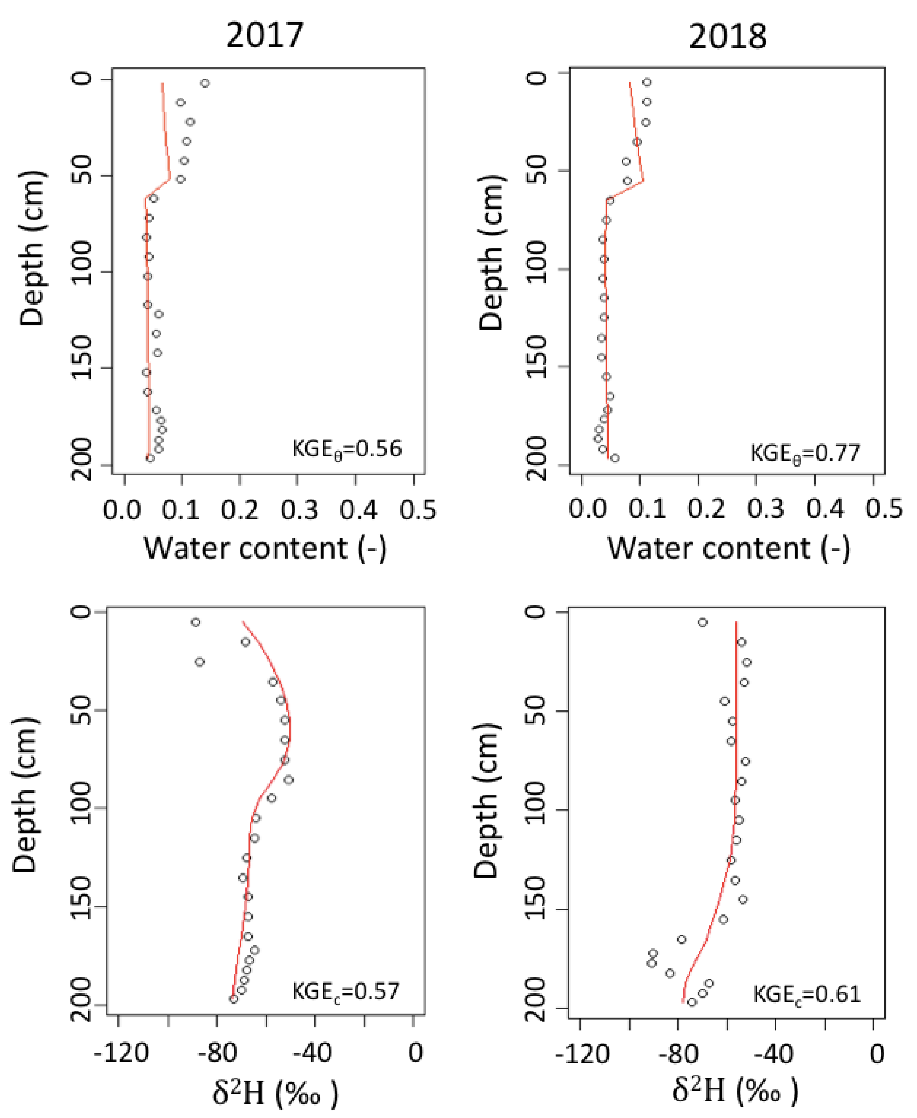
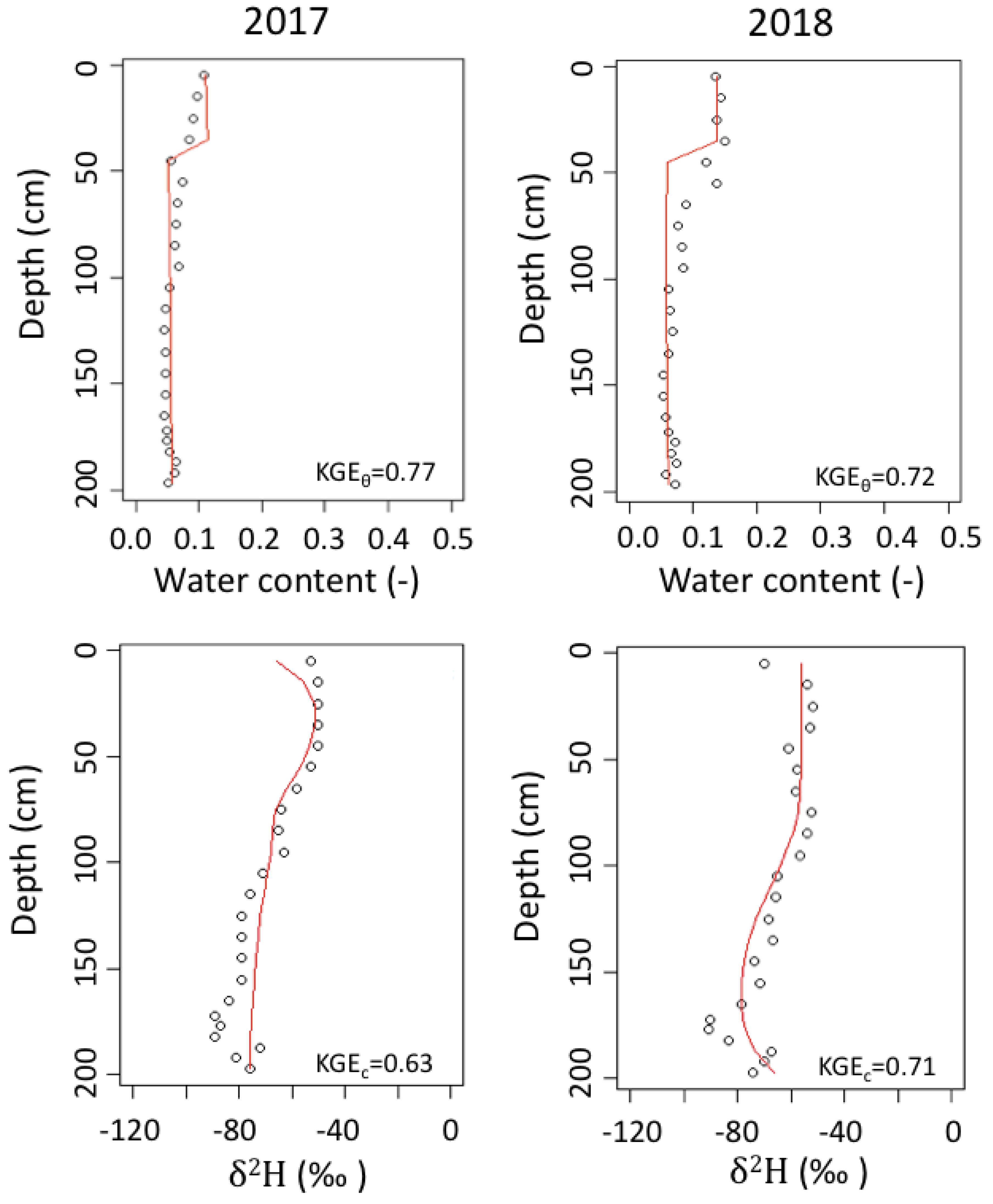
3.3. Field Case Study

Under real conditions, using one water content and pore water isotope composition depth profile from a single time to calibrate the model was also found to be a reliable approach in this work. Water content profiles (KGE_θ from 0.56 to 0.77) and δ²H profiles (KGE_c from 0.57 to 0.71) were satisfactorily reproduced (Figure 4 and Figure 5). The KGE_tot values that were obtained for the validation model period (i.e., 2018) are of the same order of magnitude as those for the calibration period (i.e., 2017), for sites SLA and SLB. For SLA, if the first three measurements (which represent the first 15 cm below the surface level) are not considered, the KGE_tot increases from 0.57 to 0.75 in 2017 and from 0.69 to 0.83 in 2018, mainly due to KGE_c increasing. We suspect that the depleted values measured at 5 and 15 cm depths correspond to two small snowfall events (the first totally melted and the second partially melted on SLA), which occurred on 19 November and 16 November 2017, respectively, a few days before soil profile sampling. The monthly collection of precipitation isotope data does not allow the conditions in the top centimeters of the soil profile to be accurately reproduced. With an increasing infiltration depth, water gets mixed with the pore water previously present in the soil, leading to the following loss of its initial isotopic signal and the convergence toward a mean value, which explains the better results obtained at a greater depth. For SLB, we do not observe this increase in KGE_c. If we look more closely at the pore water isotope profile (Figure 5), the two snowfall events mentioned above are not evident; rather, measurements in the upper 15 cm are very close to the average precipitation composition in November (δ²H = −75‰). SLB is located in a pine forest. Interception by the trees, and the needles and biomass cover on the soil could explain these results, by their not allowing small precipitation events to directly infiltrate into the soil.

The soil hydraulic parameters obtained for sites SLA and SLB are different for the two horizons considered (

Table 4. Best set of soil hydraulic parameters obtained for sites SLA and SLB.

		n	α	Ks	F	Smin	Smax	λ
		(-)	(m−1)	(ms−1)	(-)	(-)	(-)	(m)
SLA	Horizon 1	1.87	11.32	5.46 × 10−3	0.21	0.02	0.44	0.01
	Horizon 2	1.89	26.3	2.74 × 10−3	0.36	0.02	0.24	0.01
SLB	Horizon 1	1.51	20.35	8.26 × 10−3	0.28	0.04	0.54	0.01
	Horizon 2	2.16	10.61	9.49 × 10−3	0.39	0.04	0.37	0.01

), even if, for both sites, horizon 2 had no organic matter and the same granulometry. Vegetation affects the soil structure and its stability at different scales and through various direct and indirect mechanisms [55]. By penetrating the soil, roots form macropores which favor fluid transport. They also create failure zones, which contribute to fragmentation of the soil and the formation of aggregates, thus modifying soil hydraulic properties.

The mean annual groundwater recharge values obtained for sites SLA and SLB using the proposed method (

Table 5. Annual simulated groundwater recharge, evaporation, and transpiration values for sites SLA and SLB.

		Recharge	Evaporation	Transpiration
		(mm)	(mm)	(mm)
SLA	2017	429	307	117
	2018	261	220	75
SLB	2017	456	215	217
	2018	257	181	118

), 345 mm and 357 mm, respectively, are consistent with previous studies [24]. As expected, recharge values and the repartition between evaporation and transpiration are different between the sites due to differences in vegetation. The role of evaporation is greater at site SLA, which is located in grassland, and the role of transpiration is greater at site SLB, which is located in a pine forest.

4. Conclusions

In this study, we investigated the possibility of calibrating a soil water transport model to estimate groundwater recharge using only one water content and pore water isotope composition depth profile from a single sampling time. By conducting sensitivity analyses, we highlighted the difficulties in accurately calibrating the soil model. Indeed, the interactions between soil hydraulic parameters play a fundamental role, and various combinations can lead to similar groundwater recharge simulations. Combining water content and tracer data in a multi-objective calibration approach helped to constrain soil hydraulic property determination, as the influence of soil hydraulic parameters for the two types of data was found to differ. The value of pore water isotope information for appropriate soil water transport model parameterization was demonstrated. For sandy soils, accurate calibration is possible without temporally-continuous monitoring data, using only water content and pore water isotopic composition profiles measured on a single date. However, even if not continuous, multi-temporal data improve model calibration, especially pore water isotope data. Indeed, monthly water content and pore water isotope composition monitoring in the first horizon provides as much information as daily water content monitoring in both horizons. We therefore encourage field monitoring methods to develop in this direction. More generally, it is important that the choice of data used for soil hydraulic parameter calibration be made in accordance with the objectives of the model.

References

1. Aeschbach, W.; Gleeson, T. Regional strategies for the accelerating global problem of groundwater depletion. Nat. Geosci. 2012, 5, 853–861. [Google Scholar] [CrossRef]
2. Taylor, R.; Scanlon, B.; Doell, P.; Rodell, M.; van Beek, R.; Wada, Y.; Longuevergne, L.; Leblanc, M.; Famiglietti, J.S.; Edmunds, M.; et al. Ground water and climate change. Nat. Clim. Chang. 2013, 3, 322–329. [Google Scholar] [CrossRef] [Green Version]
3. Famiglietti, J. The global groundwater crisis. Nat. Clim. Chang. 2014, 4, 945–948. [Google Scholar] [CrossRef]
4. Farthing, M.W.; Ogden, F. Numerical Solution of Richards’ Equation: A Review of Advances and Challenges. Soil Sci. Soc. Am. J. 2017, 81, 1257–1269. [Google Scholar] [CrossRef] [Green Version]
5. Corwin, D.L.; Hopmans, J.; de Rooij, G.H. From Field- to Landscape-Scale Vadose Zone Processes: Scale Issues, Modeling, and Monitoring. Vadose Zo. J. 2006, 5, 129–139. [Google Scholar] [CrossRef]
6. Mermoud, A.; Xu, D. Comparative Analysis of Three Methods to Generate Soil Hydraulic Functions. Soil Tillage Res. 2006, 87, 89–100. [Google Scholar] [CrossRef]
7. Isch, A.; Montenach, D.; Hammel, F.; Ackerer, P.; Coquet, Y. A Comparative Study of Water and Bromide Transport in a Bare Loam Soil Using Lysimeters and Field Plots. Water 2019, 11, 1199. [Google Scholar] [CrossRef] [Green Version]
8. Ritter, A.; Hupet, F.; Muñoz-Carpena, R.; Lambot, S.; Vanclooster, M. Using inverse methods for estimating soil hydraulic properties from field data as an alternative to direct methods. Agric. Water Manag. 2003, 59, 77–96. [Google Scholar] [CrossRef]
9. Mertens, J.; Stenger, R.; Barkle, G.F. Multiobjective Inverse Modeling for Soil Parameter Estimation and Model Verification. Vadose Zo. J. 2006, 5, 917–933. [Google Scholar] [CrossRef]
10. Groh, J.; Stumpp, C.; Lücke, A.; Pütz, T.; Vanderborght, J.; Vereecken, H. Inverse Estimation of Soil Hydraulic and Transport Parameters of Layered Soils from Water Stable Isotope and Lysimeter Data. Vadose Zo. J. 2018, 17. [Google Scholar] [CrossRef] [Green Version]
11. Pachepsky, Y.; Smettem, K.; Vanderborght, J.; Herbst, M.; Vereecken, H.; Wösten, H. Reality and Fiction of Models and Data in Soil Hydrology. In Unsaturated-zone Modeling: Progress, Challenges and Applications; Feddes, R.A., de Rooij, G.H., van Dam, J.C., Eds.; Springer: New York, NY, USA, 2004; Volume 6, pp. 233–260. [Google Scholar]
12. Lu, X.; Jin, M.; van Genuchten, M.T.; Wang, B. Groundwater Recharge at Five Representative Sites in the Hebei Plain, China. Groundwater 2011, 49, 286–294. [Google Scholar] [CrossRef] [PubMed]
13. Wang, T.; Franz, T.E.; Yue, W.; Szilagyi, J.; Zlotnik, V.A.; You, J.; Chen, X.; Shulski, M.D.; Young, A. Feasibility analysis of using inverse modeling for estimating natural groundwater recharge from a large-scale soil moisture monitoring network. J. Hydrol. 2016, 533, 250–265. [Google Scholar] [CrossRef]
14. Wohling, T.; Vrugt, J.A.; Barkle, G.F. Comparison of Three Multiobjective Optimization Algorithms for Inverse Modeling of Vadose Zone Hydraulic Properties. Soil Sci. Soc. Am. J. 2008, 72, 305–319. [Google Scholar] [CrossRef] [Green Version]
15. Groh, J.; Puhlmann, H.; Wilpert, K. Calibration of a soil-water balance model with a combined objective function for the optimization of the water retention curve. Hydrol. Wasserbewirtsch. 2013, 57, 152–162. [Google Scholar]
16. Abbasi, F.; Simunek Jirka, J.; Feyen, J.; Shouse, P.J. Simultaneous Inverse Estimation of Soil Hydraulic and Solute Transport Parameters from Transient Field Experiments: Homogeneous Soil. Am. Soc. Agric. Eng. 2003, 46, 1085–1095. [Google Scholar] [CrossRef] [Green Version]
17. Stumpp, C.; Stichler, W.; Kandolf, M.; Šimůnek, J. Effects of Land Cover and Fertilization Method on Water Flow and Solute Transport in Five Lysimeters: A Long-Term Study Using Stable Water Isotopes. Vadose Zone J. 2012, 11. [Google Scholar] [CrossRef]
18. Sprenger, M.; Volkmann, T.H.M.; Blume, T.; Weiler, M. Estimating flow and transport parameters in the unsaturated zone with pore water stable isotopes. Hydrol. Earth Syst. Sci. 2015, 19, 2617–2635. [Google Scholar] [CrossRef] [Green Version]
19. Koeniger, P.; Leibundgut, C.; Link, T.; Marshall, J.D. Stable isotopes applied as water tracers in column and field studies. Org. Geochem. 2010, 41, 31–40. [Google Scholar] [CrossRef]
20. Zimmermann, U.; MüNnich, K.O.; Roether, W. Downward Movement of Soil Moisture Traced by Means of Hydrogen Isotopes. In Isotopes in Hydrology; IAEA, Isotopes in Hydrology: Vienna, Austria, 14–18 November 1966; International Atomic Energy Agency: Vienna, Austria, 1967; pp. 567–585. [Google Scholar]
21. Gehrels, J.C.; Peeters, J.E.M.; Vries, J.J.D.E.; Dekkers, M. The mechanism of soil water movement as inferred from 18O stable isotope studies. Hydrol. Sci. J. 1998, 43, 579–594. [Google Scholar] [CrossRef] [Green Version]
22. Souchez, R.; Lorrain, R.; Tison, J.L. Stable water isotopes and the physical environment. Belgeo. Revue Belge Géographie 2002, 2, 133–144. [Google Scholar] [CrossRef] [Green Version]
23. Goblet, P. Simulation D’écoulement et de Transport Miscible en Milieu Poreux et Fracturé; Manual: Fontainebleau, France, 2010. [Google Scholar]
24. Campolongo, F.; Cariboni, J.; Saltelli, A. An effective screening design for sensitivity analysis of large models. Environ. Model. Softw. 2007, 22, 1509–1518. [Google Scholar] [CrossRef]
25. Sobol, I.M. Global sensitivity indices for nonlinear mathematical models and their Monte Carlo estimates. Math. Comput. Simul. 2001, 55, 271–280. [Google Scholar] [CrossRef]
26. Larocque, M.; Meyzonnat, G.; Ouellet, M.A.; Graveline, M.H.; Gagné, S.; Barnetche, D.; Dorner, S. Projet de connaissance des eaux souterraines de la zone de Vaudreuil-Soulanges; Rapport Final déposé au Ministère du Développement durable, de l’Environnement et de la Lutte Contre les Changements Climatiques: Quebec, QC, Canada, 2015. [Google Scholar]
27. Mattei, A.; Barbecot, F.; Guillon, S.; Goblet, P.; Hélie, J.-F.; Meyzonnat, G. Improved accuracy and precision of water stable isotope measurements using the direct vapour equilibration method. Rapid Commun. Mass Spectrom. 2019, 33, 1613–1622. [Google Scholar] [CrossRef] [PubMed]
28. Mesinger, F.; DiMego, G.; Kalnay, E.; Mitchell, K.; Shafran, P.C.; Ebisuzaki, W.; Jović, D.; Woollen, J.; Rogers, E.; Berbery, E.H.; et al. North American Regional Reanalysis. Bull. Am. Meteorol. Soc. 2006, 87, 343–360. [Google Scholar] [CrossRef] [Green Version]
29. Folk, R.L.; Ward, W.C. Brazos River bar: a study in the significance of grain size parameters. J. Sediment. Petrol. 1957, 27, 3–26. [Google Scholar] [CrossRef]
30. Mualem, Y. A new model for predicting the hydraulic conductivity of unsaturated porous media. Water Resour. Res. 1976, 12, 513–522. [Google Scholar] [CrossRef] [Green Version]
31. Van Genuchten, M.T. A Closed Form Equation for Predicting the Hydraulic Conductivity of Unsaturated Soils 1. Soil Sci. Soc. Am. J. 1980, 44, 892–898. [Google Scholar] [CrossRef] [Green Version]
32. Feddes, R.A.; Kowalik, P.; Kolinska-Malinka, K.; Zaradny, H. Simulation of field water uptake by plants using a soil water dependent root extraction function. J. Hydrol. 1976, 31, 13–26. [Google Scholar] [CrossRef]
33. Šimůnek, J.; Šejna, M.; Saito, H.; Sakai, M.; van Genuchten, M.T. The HYDRUS-1D Software Package for Simulating the One-Dimensional Movement of Water, Heat, and Multiple Solutes in Variably-Saturated Media; University of California Riverside: Riverside, CA, USA, 2013. [Google Scholar]
34. Hargreaves, G.H.; Samani, Z.A. Estimating Potential Evapotranspiration. Appl. Eng. Agric. 1982, 1, 96–99. [Google Scholar]
35. Ritchie, J.A. Model for Predicting Evaporation From a Low Crop With Incomplete Cover. Water Resour. Res. 1972, 8, 1204–1213. [Google Scholar] [CrossRef] [Green Version]
36. Sutanto, S.; Wenninger, J.; Coenders-Gerrits, M.; Uhlenbrook, S. Partitioning of evaporation into transpiration, soil evaporation and interception: A comparison between isotope measurements and a HYDRUS-1D model. Hydrol. Earth Syst. Sci. 2012, 16, 2605–2616. [Google Scholar] [CrossRef] [Green Version]
37. Valéry, A. Modélisation Précipitations–Débit sous Influence Nivale: Elaboration d’un Module Neige et Evaluation sur 380 Bassins Versants. Ph.D. Thesis, AgroParisTech, Antony, France, 2010. [Google Scholar]
38. Vanderborght, J.; Vereecken, H. One-Dimensional Modeling of Transport in Soils with Depth-Dependent Dispersion, Sorption and Decay. Vadose Zone J. 2007, 6, 140–148. [Google Scholar] [CrossRef]
39. Gonfiantini, R. Chapter 3—Environmental isotopes in lake studies. In The Terrestrial Environment, B; Fritz, P., Fontes, J.C., Eds.; Handbook of Environmental Isotope Geochemistry; Elsevier: Amsterdam, The Netherlands, 1986; pp. 113–168. ISBN 978-0-444-42225-5. [Google Scholar]
40. Skrzypek, G.; Mydłowski, A.; Dogramaci, S.; Hedley, P.; Gibson, J.J.; Grierson, P.F. Estimation of evaporative loss based on the stable isotope composition of water using Hydrocalculator. J. Hydrol. 2015, 523, 781–789. [Google Scholar] [CrossRef] [Green Version]
41. Gat, J.R.; Levy, Y. Isotope hydrology of inland Sabkhas in the Bardawil area. Sinai. Limnol. Oceanogr. 1978, 23, 841–850. [Google Scholar] [CrossRef]
42. Gibson, J.J.; Birks, S.J.; Edwards, T.W.D. Global prediction of δA and δ2H-δ18O evaporation slopes for lakes and soil water accounting for seasonality. Glob. Biogeochem. Cycles 2008, 22, GB2031. [Google Scholar] [CrossRef]
43. Horita, J.; Wesolowski, D.J. Liquid-vapor fractionation of oxygen and hydrogen isotopes of water from the freezing to the critical temperature. Geochim. Cosmochim. Acta 1994, 58, 3425–3437. [Google Scholar] [CrossRef]
44. Gat, J.R. Stable Isotopes of Fresh and Saline Lakes BT—Physics and Chemistry of Lakes; Lerman, A., Imboden, D.M., Gat, J.R., Eds.; Springer: Berlin/Heidelberg, Germany, 1995; pp. 139–165. ISBN 978-3-642-85132-2. [Google Scholar]
45. Beven, K. A manifesto for the equifinality thesis. J. Hydrol. 2006, 320, 18–36. [Google Scholar] [CrossRef] [Green Version]
46. Saltelli, A. Sensitivity Analysis for Importance Assessment. Risk Anal. 2002, 22, 579–590. [Google Scholar] [CrossRef]
47. Usher, W.; Herman, J.; Mutel, C. SALib: Sensitivity Analysis Library in Python (Numpy). Contains Sobol, Morris, Fractional Factorial and FAST methods. 2015. Available online: http://SALib.github.io/SALib/ (accessed on 1 March 2019).
48. Kling, H.; Fuchs, M.; Paulin, M. Runoff conditions in the upper Danube basin under an ensemble of climate change scenarios. J. Hydrol. 2012, 424–425, 264–277. [Google Scholar] [CrossRef]
49. McKay, M.D.; Beckman, R.J.; Conover, W.J. A Comparison of Three Methods for Selecting Values of Input Variables in the Analysis of Output from a Computer Code. Technometrics 1979, 21, 239–245. [Google Scholar]
50. Vrugt, J.A.; ter Braak, C.J.F.; Clark, M.P.; Hyman, J.M.; Robinson, B.A. Treatment of input uncertainty in hydrologic modeling: Doing hydrology backward with Markov chain Monte Carlo simulation. Water Resour. Res. 2008, 44, W00B09. [Google Scholar] [CrossRef] [Green Version]
51. Mannschatz, T.; Dietrich, P. Model Input Data Uncertainty and Its Potential Impact on Soil Properties. In Sensitivity Analysis in Earth Observation Modelling; Petropoulos, G., Srivastava, P.K., Eds.; Elsevier: Oxford, UK, 2017; pp. 25–52. [Google Scholar]
52. Gebler, S.; Franssen, H.-J.; Pütz, T.; Post, H.; Schmidt, M.; Vereecken, H. Actual evapotranspiration and precipitation measured by lysimeters: A comparison with eddy covariance and tipping bucket. Hydrol. Earth Syst. Sci. 2015, 19, 2145–2161. [Google Scholar] [CrossRef] [Green Version]
53. Hoffmann, M.; Schwartengräber, R.; Wessolek, G.; Peters, A. Comparison of simple rain gauge measurements with precision lysimeter data. Atmos. Res. 2016, 174–175, 120–123. [Google Scholar] [CrossRef]
54. Peters-Lidard, C.; Mocko, D.M.; Garcia, M.; Santanello, J.; Tischler, M.A.; Susan Moran, M.; Wu, Y. Role of precipitation uncertainty in the estimation of hydrologic soil properties using remotely sensed soil moisture in a semiarid environment. Water Resour. Res. 2008, 44, W05S18. [Google Scholar] [CrossRef] [Green Version]
55. Angers, D.A.; Caron, J. Plant-induced Changes in Soil Structure: Processes and Feedbacks. Biogeochemistry 1998, 42, 55–72. [Google Scholar] [CrossRef]
Figure 1. Results of the Morris method sensitivity analysis for output groundwater recharge.
Water 12 00393 g001
Figure 2. Results of the Sobol method sensitivity analysis for different model outputs: (a) groundwater recharge (1096 days of simulation); (b) water content profile after 1044 days of simulation*; and (c) pore water isotope profile after 1044 days of simulation*. S1 is shown in black and ST is shown in gray. Soil hydraulic parameters are ranked by decreasing influence. * 1044 days of simulation correspond to 9 November 2018. Results were checked to be independent of the chosen day.
Water 12 00393 g002
Figure 3. Annual cumulated groundwater recharge values for 2017 (a) and 2018 (b). Results of the synthetic case are presented as continuous black lines. The five best sets of parameter results are presented as gray lines. Kling–Gupta efficiency (KGE) is calculated for the synthetic case results and the best set of soil hydraulic parameter results (black dashed line).
Water 12 00393 g003
Figure 4. Observed (circles) and simulated (lines) water content (top) and δ2H (bottom) soil profiles at site SLA, with the best parameter set.
Water 12 00393 g004
Figure 5. Observed (circles) and simulated (lines) water content (top) and δ2H (bottom) soil profiles at site SLB with the best parameter set.
Water 12 00393 g005