Nossana Spring (Northern Italy) under Climate Change: Projections of Future Discharge Rates and Water Availability


Dipartimento di Scienze della Terra “Ardito Desio”, Università degli Studi di Milano, 20133 Milan, Italy
*
Author to whom correspondence should be addressed.
Water 2020, 12(2), 387; https://doi.org/10.3390/w12020387
Submission received: 29 November 2019
/
Revised: 24 January 2020
/
Accepted: 28 January 2020
/
Published: 1 February 2020
(This article belongs to the Special Issue Hydroclimatic Variability at Local, Regional, and Global Scales)
Abstract
:Nossana represents an important pre-Alpine karst spring for drinking supply, sustaining a water distribution system serving 300,000 people. The goal of this study was to project Nossana discharges and evaluate potential supply limits for four future periods (2021–2040, 2041–2060, 2061–2080, 2081–2100). Bias-corrected Regional Climate Models (RCMs), part of the EURO-CORDEX experiment and forced by three emission scenarios (RCP2.6, RCP4.5, RCP8.5), were evaluated, statistically downscaled, and used as input in a calibrated rainfall-runoff model ensemble. For each emission scenario, the calibrated model ensemble considered three RCMs and ten rainfall-runoff parameterizations. Projected ensemble mean discharges are lower than observations (3%–23%) for all RCPs, though they do not show a clear trend between the four time periods. Days characterized by discharges lower than actual water demand are projected to decrease, except for the RCP8.5 emission scenarios and the period 2081–2100. Conversely, the same consecutive days are expected to increase after 2060 for all emission scenarios. These results reflect the projected precipitation trend, characterized by longer, drier summer periods and wetter autumns in comparison to today’s climate. Also, they indicate a possible need for alternative drinking water resources. The proposed methodology was demonstrated to deliver useful quantitative information for water management in the mid- long-term period.
1. Introduction
Karst springs play a fundamental role in large-scale human water supply, both from a strategic and socio-economic point of view [1]. Quantifying actual and future project spring discharges is extremely important to manage water resources in karstic areas, especially in view of the effects related to climate change. According to the Intergovernamental Panel on Climate Change (IPCC), the mean temperature is expected to increase globally throughout the 21st century, with a consequent increase in the frequency and magnitude of heat waves, drought periods and intense precipitation events in many regions of the world [2]. The prediction of the response to climate change in hydrogeological systems becomes vital, especially if exploited for drinking water supply [3] or the sustainability of groundwater dependent ecosystems [4].
The application of traditional groundwater flow models for the prediction of fractured media is complicated due to the duality of the flow systems [5]; this is particularly true for karst systems [6,7]. A typical karst system is formed by a fractured rock matrix, which includes both diagenetic rock micro pores and small fractures of tectonic origin, as well as a network of widely articulated karst conduits [1,8]. This dual nature leads to a hybrid flow behavior, Darcian within the rock matrix, and turbulence in the conduits. In addition, flow in the conduits can be assimilated to full pipe (pressurized) flow or to free surface flow, based on the channel saturation. Attempts to define physically based, distributed models incorporating some or all of these characteristics have been made by many authors [9,10,11,12,13,14,15]. However, the definition of a conceptual model that could depict the system heterogeneity reliably, in terms of both 3D geometry and parameterization, can be very data demanding, time consuming, and costly [16]. Speleological exploration (e.g., [17]) and artificial tracers (e.g., [18]) can furnish information on spring catchment areas and the main geometric properties of the karst system. Additional insights regarding different water sources and water residence time in the aquifer can be derived from natural tracer analyses, such as water isotopes, major ions, trace elements, and dissolved organic carbon (e.g., [19,20,21,22,23]). In-situ hydraulic methods, such as pumping tests, can provide knowledge on the degree of confinement of the aquifer and its quantitative parameters (e.g., [24,25]). Non-invasive geophysical methods can also be used to gather information on aquifer geometry and boundaries (e.g., electric and seismic methods, [26,27]), to identify major voids and conduits (e.g., gravimetric and geomagnetical methods, [28]), and to recognize preferential infiltration pathways (e.g., self-potential methods, [29]). In addition, to allow model calibration, a continuous monitoring of at least precipitation and spring discharge is essential [16].
When the main goal of the study concerns the response of a karst spring to meteorological events, the continuous monitoring of precipitation and discharge could suffice for a modeling setup. Input-output models can be used to relate the precipitation contribution to the outflow through empirical equations based on lumped parameters (e.g., [30,31]), neural networks (e.g., [32]), or input-response functions (e.g., [33,34]). An increasing number of studies involving such modelling approaches have been documented for karst environments in recent years (e.g., [35,36,37,38,39]). Due to the lack of physical processes representation, a limitation of these models concerns their loss of reliability if applied in conditions that largely differ from calibration [40,41]. Parameter transferability has been largely tested (e.g., [42,43,44]), suggesting an increase in simulation errors and uncertainties with increasing differences in mean rainfall. Also, performance losses appear larger when transferring parameters from wet to dry periods than vice versa. Vaze et al. [42] concluded that calibrated models could be used for climate change impact studies if mean rainfall changes between future and calibration periods fall within a −15% to +20% range.
Climate projections are derived from Global Circulation Models (GCMs) forced according to the representative concentration pathways (RCP, [45]) proposed by the IPCC [2]. Usually, these models are run at large horizontal resolutions (≥ 80 km) and are therefore not able to reproduce climate states at regional or local scales reliably [46]. To obtain climate projections at a finer resolution by reproducing the physics of the processes, dynamical downscaling through Regional Climate Models (RCMs) is performed (e.g., [47,48]). With the ongoing climate modeling experiments—for example, the Coordinated Regional Climate Downscaling Experiment (CORDEX, http://www.cordex.org/), WorldClim dataset project (http://www.worldclim.org/), and the Climate Change, Agriculture, and Food Security research program (CCAFS, http://ccafs-climate.org/downscaling/)—future climate projections are made available over several domains worldwide with a horizontal resolution of up to 12.5 km. Some studies (e.g., [49,50]) demonstrated that dynamical downscaling can be applied to achieve an even larger detail (≤4 km). However, these methods are computationally very intensive and often show performance losses over complex terrains [46,51]. The computationally inexpensive alternative is statistical downscaling, which provides a predictive framework of local conditions (with almost no bias with historical records) through statistical relationships with regional climatic aspects. The hypothesis is that the relationship between large-scale atmospheric circulation and local scale dynamics is constant [52,53,54]. Therefore, statistical downscaling allows for producing large ensembles of climate change projections for extended time periods [46,55].
The overarching goal of this study is to propose a methodological approach to evaluate possible variations in the discharge regime of a karst spring in basins affected by climate change. The selected study area is the hydrogeological basin of the Nossana Spring (northern Italy), which is heavily exploited for drinking water. Using a control data period covering 1998–2017, the specific objectives of this study are: (i) quantification of the expected changes in precipitation and temperature in the study area, for twenty-year periods till 2100, as resulting from the statistical downscaling of RCMs run under three RCPs (2.6, 4.5, 8.5); (ii) calibration and validation of a lumped-parameter model (GR4J with CemaNeige [56,57,58]) based on observed data; (iii) recognition of possible limits in the future utilization of the spring as a drinking supply based on simulated discharge and actual warning thresholds.
2. Study Area
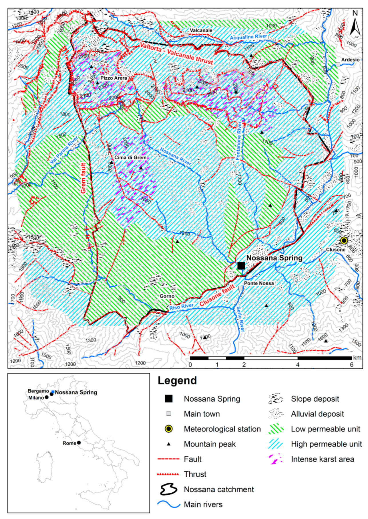
The Nossana Spring is located in the central Prealps of Seriana Valley, within the Lombardy Region of the Province of Bergamo (Northern Italy) (Figure 1). Its hydrogeological basin covers an area of about 80 km2 and is characterized by large differences in altitude, ranging from 474 m a.s.l. (Nossana Spring) to 2512 m a.s.l. (Pizzo Arera Mountain).
The spring is managed by the public company UniAcque S.p.A. and feeds the main local water distribution system, serving over 300,000 people. The observed mean annual discharge (1998–2017) is 3.77 m3 s−1. For the same period, the observed daily variability is extremely high, with values ranging from 0.55 m3 s−1 to 18.00 m3 s−1. In a single day, discharge varied up to 12 m3 s−1, suggesting high flow velocities characterizing the system.
To manage the water resource, UniAcque S.p.A. set two warning thresholds based on average water demand according to the period of the year (one threshold for the cold-wet season and one threshold for the hot-dry months). Below these discharge thresholds, there is a need to integrate the spring resources pumping water from deep wells in the Serio River Valley. This entails different issues, from costs increase to quality decrease. Moreover, nowadays the additional discharges are limited (0.50 m3 s−1). During wet, cold periods, the warning threshold is set at 1.32 m3 s−1; during dry, hot periods, the threshold is set at 1.52 m3 s−1. These two discharge rates include a share for UniAcque S.p.A. (0.80 and 1.00 m3 s−1, respectively) and a share for environmental flow and use of the downstream municipalities (0.52 m3 s−1). Water that is not used by UniAcque S.p.A. flows into the Serio River, the main watercourse of the Seriana Valley.
Many studies have defined a hypothetical hydrogeological catchment for the spring [59,60], considering the geological, geomorphological, and tectonic evidences of the area [61,62,63,64]. The karst massif that characterizes the area consists of calcareous and calcareous-silicoclastic series (medium-late Triassic). The main calcareous formation is represented by “Calcare di Esino” (middle-late Trias), constituted by deeply karstified massive or stratified limestone, with a maximum thickness of about 800 m. Karst evidences (e.g., dolines and tunnels) are mainly recognized in the western and north-eastern area of the basin. The late-Triassic marl formations with low permeability (Breno Formation, Metamorphic Bergamasco Limestone and Gorno Formation) link the massif to its southern, western, and eastern borders along the tectonic contacts with the Calcare di Esino formation. Three main fragile structures mark the limits of the massif along the northern side (“Valtorta-Valcanale thrust”), west side (“Grem fault”), and southeast side (“Clusone fault”). More specific geological information about the study area can be found in literature [63,65,66].
According to Vigna and Banzato [67], based on the geological and hydrographic characteristics described above, Nossana can be classified as a karst spring fed by a dominant drainage system. These systems are usually characterized by a high permeability, which is linked to a considerable karstification process. The outflow network is well-organized with a series of main natural tunnels and secondary conduits that rapidly discharge incoming infiltration water. The most important features are the very low or complete absence of a classic phreatic zone (indeed, the presence of a phreatic zone has not been verified for Nossana yet) and the very high flow velocity.
The climate of the study area is wet and temperate. According to data recorded at the meteorological station of Clusone (591 m a.s.l.), located at around 4 km east of Nossana Spring, rainfall is distributed throughout the year. Mean annual rainfall calculated for the period 1998–2017 is 1384 mm, with November as the wettest month (average of 160 mm) and January as the driest (average of 65 mm). May, June, October, and November yield similar amounts of rainfall. Conversely, the winter lowest values indicate a change from liquid (rainfall) to solid precipitation (snow/ice). Average monthly temperatures vary between 1.4 °C (January) and 21.7 °C (July), with an overall mean annual temperature of 11.5 °C. According to Köppen–Geiger climate classification [68], the climate of the area can be classified as Cfb; namely, temperate with a wet summer, the mean temperature of the warmest month below 22 °C, and at least four months above an average of 10 °C.
3. Data
Data used to perform the study were derived from three main sources. Daily spring discharge values (m3 s−1) were provided by UniAcque S.p.A. for the period 1998–2017. Observed daily precipitation (mm), minimum and maximum temperature (°C) time series (1998–2017) were downloaded for the Clusone meteorological station from the web portal of the Regional Agency for the Environment (ARPA Lombardia, https://www.arpalombardia.it/Pages/Meteorologia/Richiesta-dati-misurati.aspx). In addition, daily time series of precipitation, minimum temperature, and maximum temperature resulting from climate simulations were extracted for the period 1970 to 2100 from selected RCM model runs of the EURO-CORDEX database. The latter were accessed through the Earth System Grid Federation (ESGF https://esgf-data.dkrz.de). In detail, bias corrected RCM model runs available at 12.5 km resolution for all emission pathways (RCP2.6, RCP4.5, RCP8.5) were selected (Table 1). This selection was done to allow a robust and coherent comparison between the projected future emission pathways, which depend on the political and economic actions that will be undertaken to reduce greenhouse gas emissions. The RCP2.6 scenario foresees that emissions will be halved from the year 2050; for RCP 4.5 this target will be reached in 2080; while according to RCP8.5 emissions will continue to increase with today’s rate [2]. The constraint to have the same models for all the RCPs limited their number; however, they include two GCMs, three different ensemble runs, and two RCMs. All models were corrected for bias by the Swedish Meteorological and Hydrological Institute (SMHI) using a distribution-based scaling method [69] based on MESAN reanalysis data (1989–2010).
4. Methods
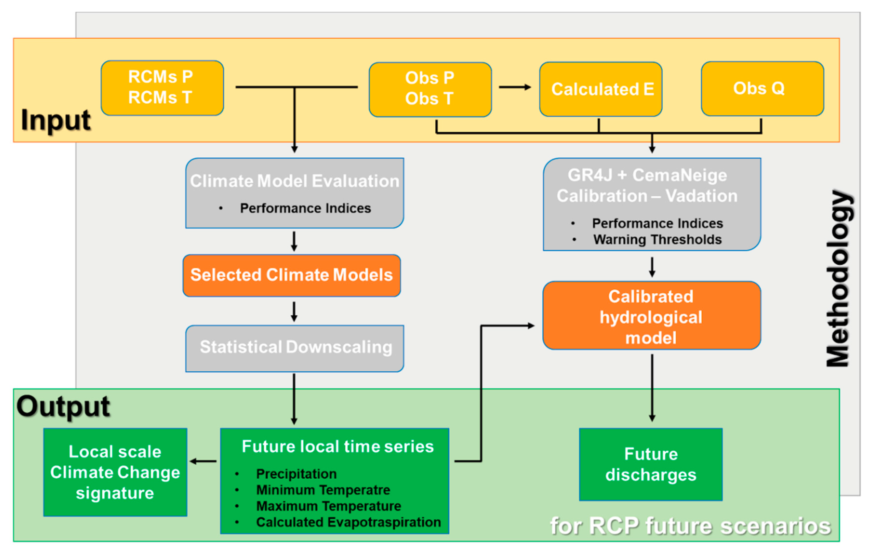
The study is based on four main steps, which are summarized in Figure 2. First, climate models are evaluated to verify their ability to reproduce the general climatology of the study area. Second, RCMs future projections are downscaled through statistical methods and local climate changes are evaluated. Third, observed time series of precipitation and temperature are used as input in a rainfall-runoff hydrologic model, which is calibrated and validated against observed discharge. Finally, the downscaled time series are used to feed the calibrated hydrologic model and possible changes in the spring discharge rate characteristics are analyzed.
4.1. Climate Models Evaluation
Daily time series of precipitation, minimum temperature, and maximum temperature were extracted for the three RCMs realizations and the three RCPs (total of nine combinations) from the grid cell where the Clusone meteorological station is located. The RCMs were evaluated by comparing their results for the control period (1998–2017) with the available observational data. Representative Concentration Pathways begin to diverge after 2005; therefore, between this date and the end of the control period, the same model, under different RCPs, could produce data with small differences. For this reason, the evaluation included all nine modeling combinations.
The evaluation consisted of the comparison of monthly rainfall and temperature climatology, and of the verification of their similarity through two performance indices. The selected indices were the Nash-Sutcliffe Efficiency (NSE—[70]) and the Mean Absolute Error (MAE). The RCMs were considered to be generally able to catch the local climatology for positive (>0.8) NSE values and MAE values lower than 20% of the mean monthly rainfall (temperature). The indices are calculated as:
where OBS refers to observations, MOD to modelled data, t indicates the time step (in this case the month), and N is the total number of time steps.
4.2. Statistical Downscaling
Precipitation and temperature data for the nine modeling combinations were statistically downscaled using a two-step approach, based on change factors and weather simulators (e.g., [71]). Assuming a stable climatology for twenty-year periods, the downscaling was performed for four time intervals (2021–2040; 2040–2060; 2061–2080; 2081–2100). Change factors [72] were calculated from daily modeled data, on a monthly (half-monthly) basis, for a selected set of rainfall (temperature) statistics, for each modeling combination and time period. For details on change factors calculation of different rainfall and temperature statistics, the reader can refer to Kilsby et al. [73]. Once calculated, change factors were applied to the same set of observed statistics to obtain values describing the local scale future behavior for each month of the year. These local scale, future statistics were used as inputs to fit a stochastic rainfall and temperature generator returning daily time series. Rainfall, minimum temperature, and maximum temperature time series were generated for each modeling combination and time interval.
4.2.1. Rainfall Generator
For future precipitation simulation, RainSim V3.1.1 [74] was used. RainSim is a rainfall generator software able to work in both single site and spatial-temporal mode. It is based on a Neymann-Scott Rectangular Pulses (NSRP) model [75,76], which manages rainfall occurrence and amount as a single process. Storms arrive as Poisson processes and each storm is characterized by a random number of rain cells, each having a certain origin delay time from the beginning of the storm, a certain duration, and a certain intensity. In single site mode—the one used in this study—to generate rainfall time series, RainSim needs to fit five internal parameters for each calendar month (Table 2). These parameters are fitted through an optimization function embedded in the software, which works based on a set of input statistics (e.g., for future periods those obtained from the change factor approach described in Section 4.2). For each month, seven statistics were used to fit the model: mean daily rainfall, daily variance, daily skew, lag-1 autocorrelation, probability of dry days (threshold 0.2 mm), probability of dry day to dry day transition, and probability of wet day to wet day transition.
4.2.2. Temperature Generator
To generate maximum and minimum temperature time series, the approach presented by Richardson [77] was adopted and implemented in the R software (www.r-project.org). The R-scripts were first developed by Camera et al. [78] and adjusted for this study. Temperature was modeled as a stochastic process with the daily mean and standard deviation conditioned on the wet and dry state of the day (threshold 0.2 mm). Richardson [77] proposed an approach in which residual time series are generated, so the first step consisted of computing the residuals for the minimum and maximum temperature time series recorded in Clusone. To do so, means and standard deviations of the 20-year time series were calculated for dry and wet days for each half-month. Going forward, a first-order Fourier series was fitted through these values, using the least squares method to obtain mean and standard deviation values for each calendar day (1–365) for both dry and wet states.
As in [77], a weak stationary generating process [79] was used to simulate time series. Only one residual time series was generated for each variable (minimum and maximum temperature) because in working with residuals the effect of the wet or dry state of the day was removed. Once the residuals time series were obtained, the daily values of minimum and maximum temperature were calculated multiplying the residual by the standard deviation and adding the mean, according to the state of day. Before back-transforming the generated residual time series into actual temperature values, standard deviation and mean were modified by applying the calculated change factors. In this way, the simulated future temperature time series were linked to the rainfall series previously generated.
4.2.3. Evaluation of the Local Climate Change Signature
A visual comparison between the monthly climatology calculated from observations and those derived from the generated time series was carried out for each time interval (2021–2040, 2041–2060, 2061–2080, 2081–2100) and RCP, to verify possible shifts in the general climate trend of the area. In addition, changes in mean annual precipitation and temperature were calculated. It was verified that mean annual rainfall changes projected by the statistical downscaling of every modelling combination fell between −15% and +20% in comparison to the control period. This is the range suggested by Vaze et al. [42] as a limit for a solid and reliable temporal transferability of lumped model parameter sets.
4.3. Hydrologic Modelling
To model the spring response to precipitation events, the daily rainfall-runoff (here applied as rainfall-discharge) four-parameter GR4J model (Génie Rural Journalier with 4 parameters, [56]), extended with the CemaNeige snow accounting routine [57,58,80], was applied. Model calibration, validation, and future discharge simulations were performed using the open-source AirGR 1.4.3.52 package [81,82] in the R 3.5.3 software (www.r-project.org). GR4J was selected since it is under continuous development and widely known (e.g., [83,84]), as well as being characterized by a parsimonious but flexible structure that allows for the simulation of complex catchments [85]. Also, it was already applied and verified in karst environments (e.g., [38,85,86]).
4.3.1. Model Description
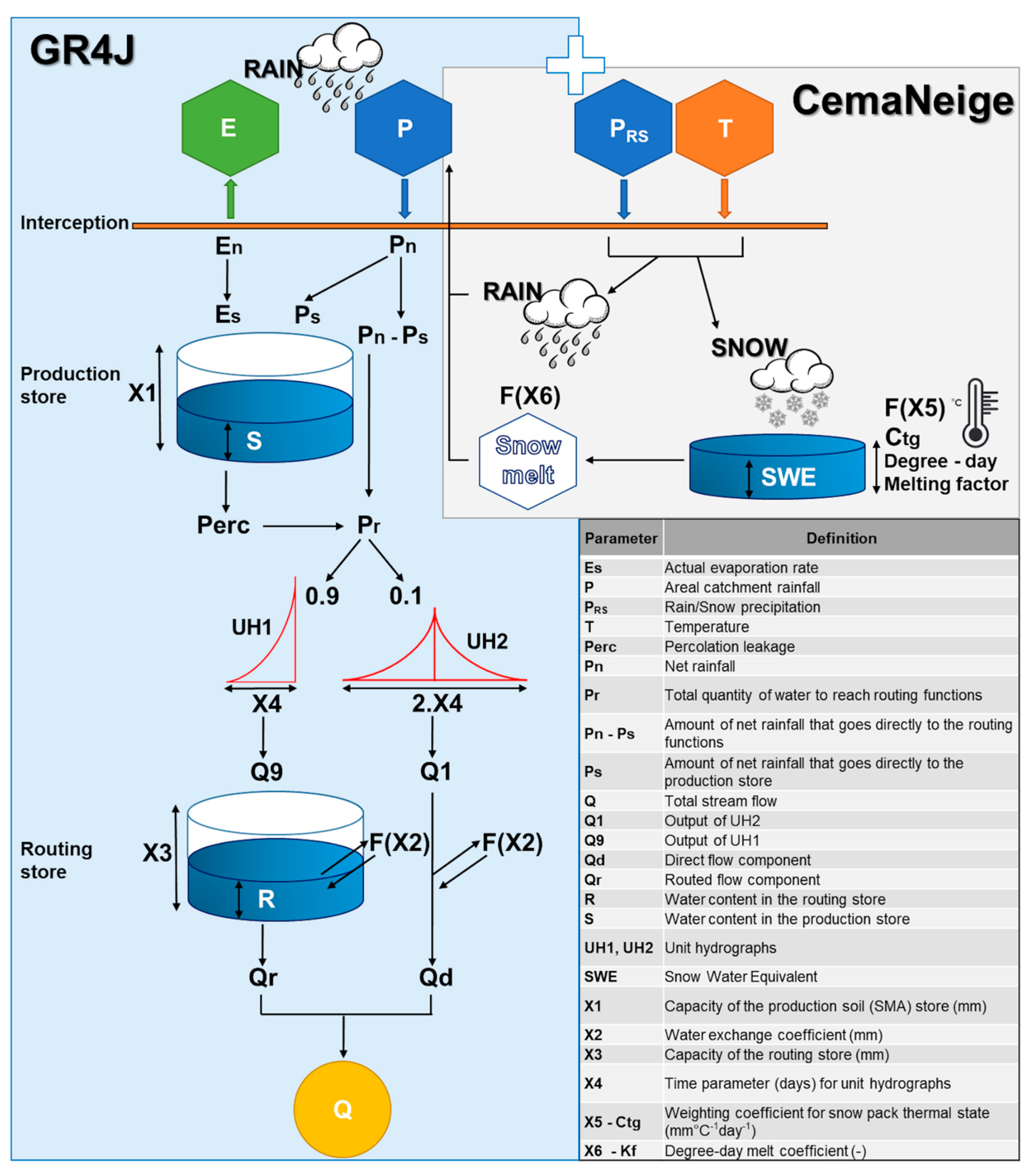
A schematic representation of the model is presented in Figure 3. Model inputs are time series of daily precipitation (P) and daily potential evapotranspiration (E). The model structure consists of two non-linear reservoirs, the production store and the routing store, a delay function element, and a groundwater exchange component. From the inputs, a net rainfall (Pn) or a net evapotranspiration (En) is calculated. In case of net evapotranspiration, a quantity Es (actual evapotranspiration) is subtracted from the production store. In case of net rainfall (Pn), this is split into two components. The first component (Ps) is added to the production store, while the second component is added to the release from the production store (Perc) to give a total amount Pr. Ps, Es, and Perc are defined as functions of the production store level (S) and of its maximum capacity (X1). Pr is then split into two fixed amounts; 0.9Pr is routed by the unit hydrograph HU1 so that a quantity Q9 enters the routing store, while 0.1Pr is routed through the unit hydrograph HU2 so that a quantity Q1 is available for fast drainage towards the basin outlet. The unit hydrographs are defined based on the model parameter X4. Before reaching the outlet, Q1 could lose or gain water from interactions with groundwater, resulting in Qd. Water is also released towards the basin outlet from the routing store (Qr) based on the store level (R), its maximum capacity (X3), and interactions with groundwater. The latter are controlled by the parameter X2 (exchange coefficient). The model output discharge (Q) is given by the sum of Qr and Qd. In a karst environment the roles played by the production store and the routing store could be assimilated to those of the rock matrix and the conduits, respectively.
The CemaNeige module allowed us to account for delays in the GR4J precipitation input, transforming part of the precipitation into snowfall and simulating snow melting according to temperature data and two parameters. Model inputs are daily precipitation, minimum temperature, and maximum temperature time series, which need to be referred to a specific elevation. In addition, the distribution of the elevations within the study area is necessary. Based on these data, with an internal routine, the model divides the study area in elevation layers of equal areas and the user can optionally define a mean annual snowfall value for each. For layers with median elevations lower than 1500 m a.s.l., CemaNeige partitions precipitation (PRS) into rainfall (RAIN) and snow (SNOW) as follows:
where Tmax and Tmin are daily maximum and minimum temperature, respectively. For layers with median elevations equal or higher to 1500 m a.s.l., the model calculates the rainfall fraction as follows:
The snow fraction is calculated according to Equation (4) in this case also. Melting is then controlled by temperature and the two model parameters: Kf [-], which is the degree-day melting factor, and Ctg [mm° C−1 day−1], namely the weighting coefficient for snowpack thermal state, which describes the thermal inertia of the accumulated snow. The higher is Kf, the larger is the snowmelt; the higher is Ctg, the later snow melts. Recently, Riboust et al. [80] presented a modified and extended version of the CemaNeige module to account for the melting heterogeneity of the snow. To do so, they enriched the model with two additional parameters to simulate hysteresis cycles with a linear model. The two extra parameters define the accumulation threshold at which the Snow Cover Area (SCA) equals 100% and the melting threshold at which the SCA drops below 100%. In this study, both the standard and the hysteretic CemaNeige modules were tested.
4.3.2. Model Calibration and Validation
Regarding the inputs, potential evapotranspiration was calculated using minimum and maximum temperature records applying the Hargreaves equation [87]. For the CemaNeige module, the elevation of the Clusone meteorological station (591 m a.s.l.) was specified as the reference one. Based on the elevation distribution within the study area, five equal area layers were created (458–882, 882–1222, 1222–1518, 1518–1789, 1789–2507 m a.s.l.). For each layer, the mean annual snowfall value (45 mm, 60 mm, 100 mm, 155 mm, 200 mm, respectively) was derived, in water equivalent, from the available national and regional snowfall maps [88,89]. For the conversion between snowfall and water equivalent, the conventional 10:1 water density to snow density proportion (1 cm of snow equals 1 mm of rainfall) was applied [90].
The observation period (1998–2017) was split into three intervals: two years for model spin-up (1998–1999) and nine years each for calibration and validation (2000–2008 and 2009–2017, respectively). Ten thousand random parameter sets were generated within the ranges specified in Table 3. The ranges of the GR4J parameters correspond to the 80% confidence intervals obtained by Perrin et al. [56] calibrating the model over 429 catchments worldwide. The ranges of the CemaNeige model parameters are those suggested by Ayzel et al. [91] for Kf and Ctg. For the accumulation threshold (X7–Tacc), the mean annual snowfall of the lower elevation layer was considered to be the maximum value of the range (minimum zero). For the melting threshold (X8–Tmelt), the maximum flexibility was given to the model. The model was run with each parameter set for both 2000–2008 and 2009–2017 periods. Only parameter sets returning, for both periods, a Kling-Gupta Efficiency (KGE, [92,93]) larger than 0.7 and a Nash-Sutcliffe Efficiency [70] calculated on logarithmic values (lNSE) larger than 0.5 were retained for future simulations. KGE was selected as one of the two performance indices since it is rather complete, addressing linear correlation (r), bias (β), and variability (γ) occurring between simulated and observed discharge values. Similarly, lNSE was selected because it is the most common evaluation index for hydrologic models and in its logarithmic formulation it gives particular importance to low flow values, which are of particular interest in this study for the exploitation of the spring for drinking supply. The formulation of KGE is presented below, while for lNSE the reader can refer to Equation (1).
with:
where μ is the mean flow rate [m3 s−1], and CV is the coefficient of variation [-].
In addition, the outputs of the model obtained with the calibrated and validated parameter sets were checked against two emergency discharge thresholds, counting the days, and the maximum number of consecutive days below those discharges. Modeled values were compared with observations.
4.4. Changes in Discharge Regimes at Nossana Karst Spring
To evaluate the changes in discharge regime at Nossana karst spring, the model was run in ensemble mode with all the calibrated and validated parameter sets, and the downscaled future time series of precipitation and temperature as input. The last two years of observations (2016–2017) were used as the spin-up period. Changes in discharge regimes were analyzed mainly in terms of low flow. Variations in the number of days and consecutive days below the warning thresholds were calculated. In addition, an analysis of the general sensitivity of the spring to climate change was carried out, analyzing variations in average discharges in relation to modifications in precipitation amounts, precipitation partitioning into rain and snow, and temperature.
5. Results
5.1. Climate Models Evaluation
The results of the RCMs evaluation are presented in Table 4. Regarding precipitation, Mod_1 (see Table 1) is the model that best responds under all three RCP scenarios (divergence after 2005). Its NSE values result higher than 0.65 and the normalized MAE values lower than 15%. The other two models show larger errors and a lower fit with the observed climatology but they are generally able to represent the precipitation annual cycle, too. In addition, all models can satisfactorily catch the minimum and maximum temperature monthly climatology. NSE values are all very high (>0.95), while normalized MAE values for mean temperature range between 4% and 7%. All models were considered suitable for statistical downscaling.
5.2. Statistical Downscaling—Local Climate Change Signature
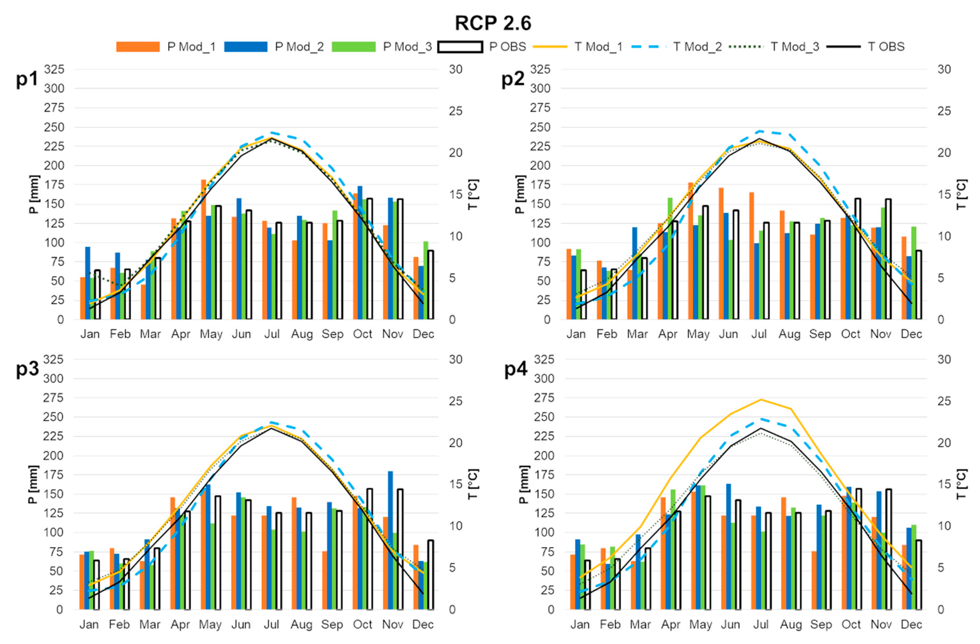
The results obtained from the statistical downscaling of the RCMs are presented by RCP scenario in twenty-year periods, to be consistent with observations (1998–2017). For convenience, the twenty-year periods 2021–2040, 2041–2060, 2061–2080, and 2081–2100 are defined as p1, p2, p3, and p4, respectively.
Projected changes in mean annual precipitation, for all models and RCPs, fall within the range suggested by Vaze et al. [42] for the application of rainfall-runoff models outside their calibration-validation conditions (Table 5). The only exception is the decrease (−18.5%) projected by Mod_1 for p2 and RCP4.5. In terms of temperature, mean annual changes range from 0.7 °C (RCP2.6, p1) to 5.8 °C (RCP8.5, p4). The actual occurrence of these changes would lead to a modification in the climatic regime of the area, according to the Köppen and Geiger classification [68]. The shift would be from Cfb to Cfa (i.e., a temperate climate characterized by wet summer and temperatures of the warmer month always higher than 22 °C). Except that for RCP8.5 and p4, the different RCMs usually agree in terms of projected temperature, while they show some differences in precipitation.
For the low emission scenario (RCP 2.6) (Figure 4), the monthly precipitation trend usually remains unchanged. Exceptions are January after 2040 and the spring season, both characterized by a slight increase in precipitation (15-20 mm). Also, Mod_1 projects a large increase of precipitation in May, for p1 and p2 (>25 mm), and an even larger decrease of precipitation in September (>50 mm), starting from p3. Temperatures in p1, p2, and p3 are projected to remain constant in the summer period, while showing a slight increase (around 1.0 °C) in the winter months. A strong increase in temperature is projected by Mod_1 in p4 for all the months of the year, up to a maximum of about 3 °C.
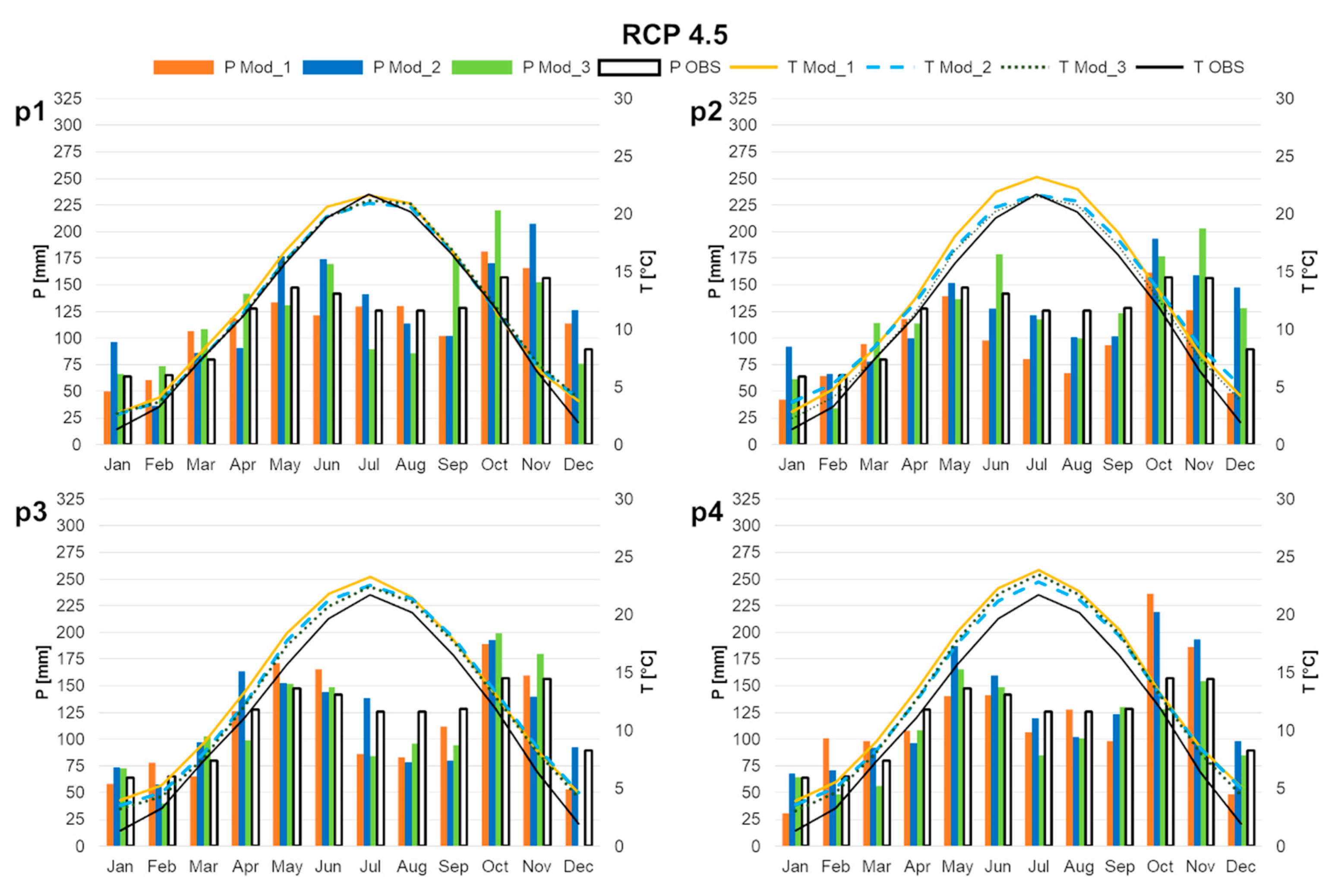
For the mid emission scenario (RCP4.5, Figure 5), in comparison to observations, the models (ensemble mean) project a slight increase in precipitation in the spring (around 20 mm, early spring in p1, shifting to May moving to p4), a marked decrease in the summer (up to 40 mm in August and 30 mm in September during p3), and another increase in autumn with peaks in October (around 40 mm in p3). The periods p2 and p3 are the most affected. Temperature trends are generally preserved, with a slightly higher increase observed in the winter months rather than in the summer period for p1 and p2. In the other two periods, changes appear quite homogeneous throughout the year, reaching up to approximately 2.5 °C.
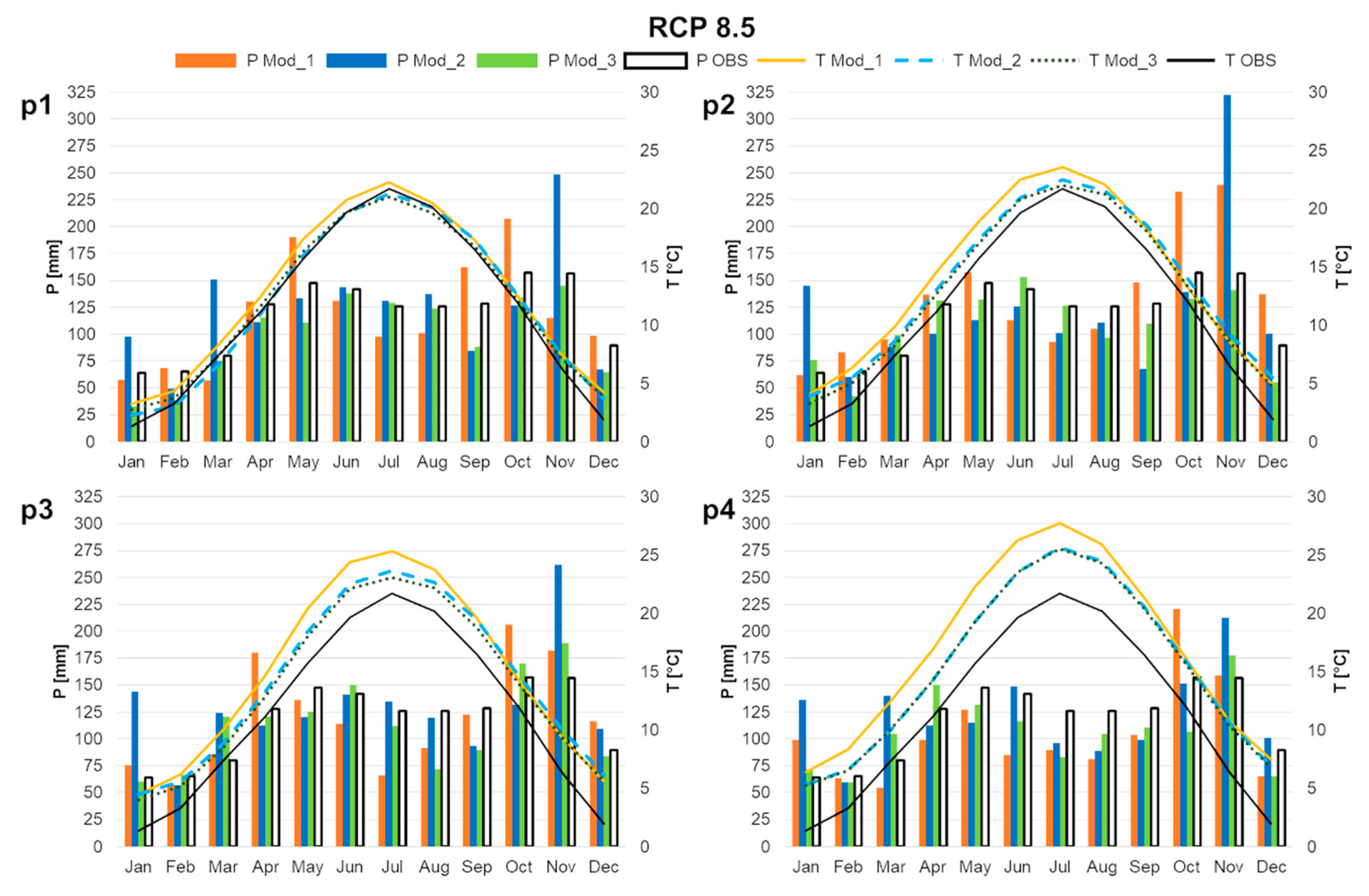
The precipitation regime of the high emission scenario (RCP8.5, Figure 6) shows large differences in comparison to observations and the other two scenarios, exhibiting an extreme autumn peak (up to 322 mm/month according to Mod_2 for November in p2), a precipitation increase in the winter months (particularly in January), and a marked decrease in the summer period (25 mm or more in July, August and September for all models in p4). Temperatures constantly increase from p1 to p4, when they show monthly values in the summer of up to 4.7 °C (ensemble mean) larger than in the control period.
5.3. Hydrologic Model Calibration and Validation
The calibration-validation procedure led to a recognition of ensembles of ten 6-parameter sets (GR4J and CemaNeige model) and eight 8-parameter sets (GR4J and CemaNeige with hysteresis) able to satisfy the established performance criteria. The ensemble of calibrated-validated sets for the 6-parameter model with the corresponding performance indices are presented in Table 6. Since no significant differences in the simulated discharges were found between the two snow modules (for conciseness the results obtained with hysteresis are not shown), the model with six parameters was preferred.
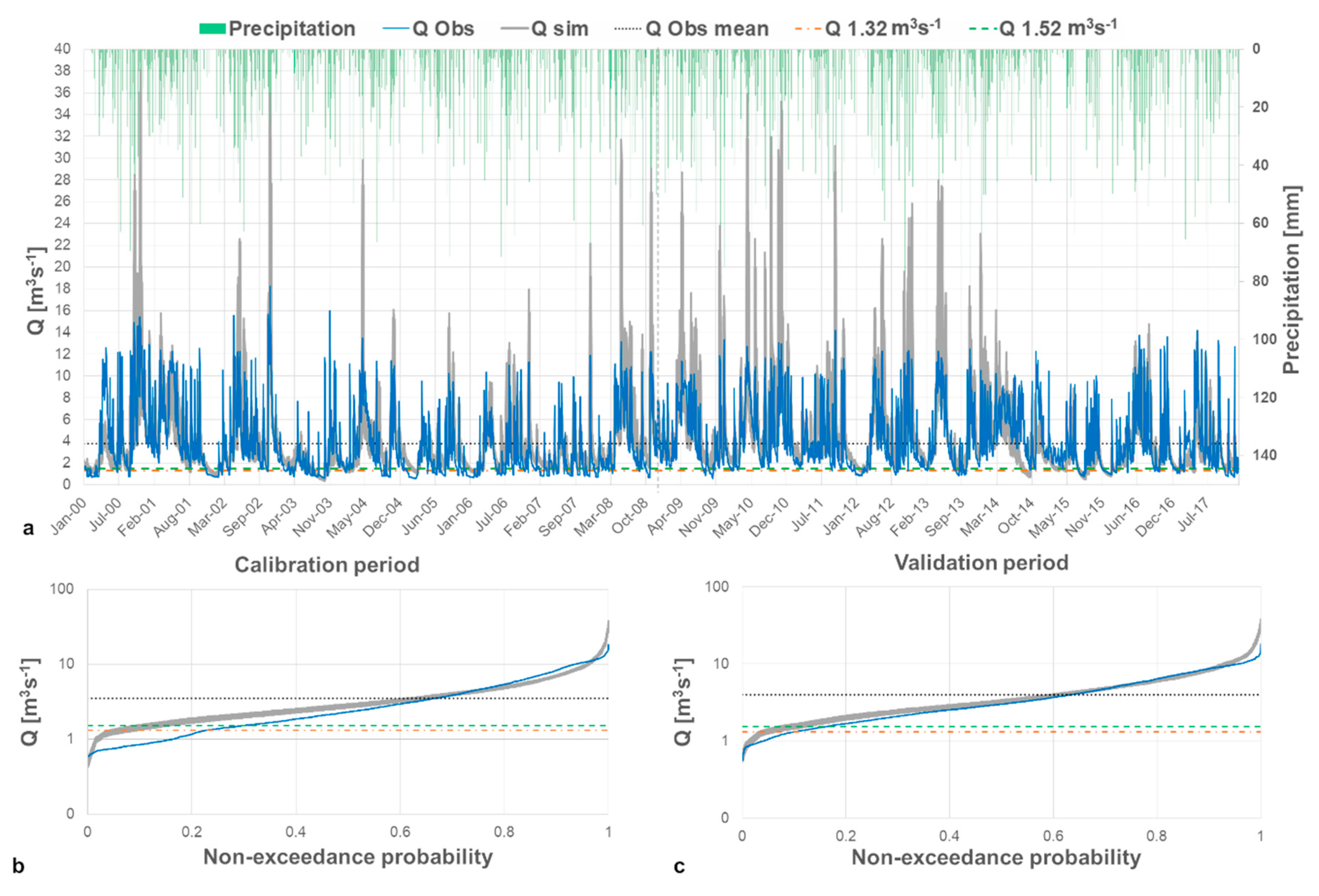
Simulated discharge time series for the calibration and validation periods are shown in Figure 7, together with the non-exceedance probabilities. From the hydrograph, simulated discharges seem to approximate low-flow observations well, while peak flows are generally overestimated. Low-flow non-exceedance probabilities are also somewhat overestimated, especially for the calibration period. This model behavior is underlined by the mean discharge values and number of days below the warning thresholds. During calibration, the simulated mean flow is on average 7.7% (9.2% for validation) higher than the observed flow (3.48 m3 s−1 and 4.00 m3 s−1 for calibration and validation, respectively). In terms of the number of days below the thresholds, the model ensemble underestimates observations in both calibration and validation period. For the calibration period, the days below the 1.32 m3 s−1 (1.52 m3 s−1) threshold are 758 (992), while for the model ensemble they range from 141 to 310 (307-513). Similarly, for the validation period there are 335 (522) observed days below the 1.32 m3 s−1 (1.52 m3 s−1) threshold, while the model ensemble simulates a number of days between 122 and 207 (216–391). The model ensemble returns better results in terms of the maximum number of consecutive days below the thresholds, which are slightly underestimated with the exception of the lower threshold during the calibration period. Specifically, for the calibration period and the 1.32 m3 s−1 (1.52 m3 s−1) threshold, this index is calculated as 10 (46) days for observations and 58–63 (35–44) days for the model ensemble. The consecutive number of days below the threshold can therefore be considered the most reliable parameter to evaluate the future behavior of the Nossana Spring and discuss its future management. It is an indicator of a critical period length, during which the service company could need additional water resources to meet the demand.
5.4. Changes in Discharge Regimes at Nossana Karst Spring
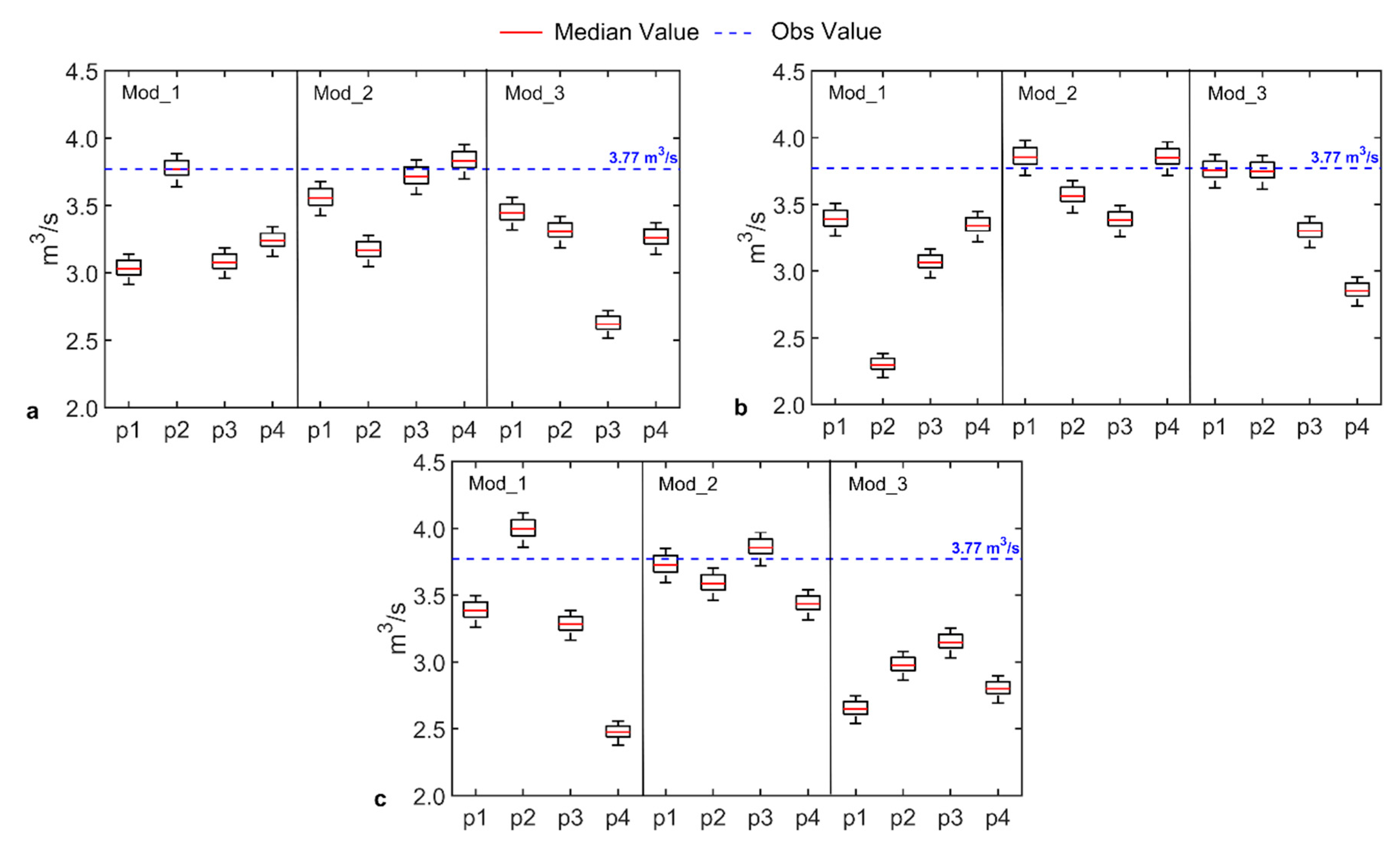
The distribution of simulated mean discharge rates for the rainfall-runoff model ensemble, presented by RCP scenario, RCM, and twenty-year period, is shown through the boxplots in Figure 8. Simulated thirty-member (RCM and rainfall-runoff) ensemble mean discharges are lower than the mean observed flow (3.77 m3 s−1) for every twenty-year period and RCP scenario, ranging from −3% (for p1 and RCP4.5) to −23% (for p4 and RCP8.5). However, a monotonous trend with time cannot be recognized. Also, the high emission scenario (RCP8.5) results in noticeably lower mean discharges than the other two RCPs only for p1 and p4.
Considering single RCPs, it is noted that the variability within the rainfall-runoff ensemble appears to be limited, while the variability between RCMs for the same period of time is much larger. Indeed, mean discharge values are strictly connected with mean annual rainfall amounts, which are extremely variable (see Table 5). For example, the mean annual rainfall decrease of 18.5% projected by Mod_2 for RCP4.5 and p2 corresponds to a 39% decrease in mean discharge. Similarly, the mean annual rainfall increase of 15.1% projected by Mod_1 for RCP8.5 and p2 corresponds to a 6% increase in mean discharge. However, although a decrease in mean annual rainfall is always closely related to a decrease in mean annual discharge, an increase in rainfall does not necessary lead to an increase in discharge. This lacking increase is related to a simultaneous increase in temperature and therefore evapotranspiration rates. As an example, for Mod_2 and RCP8.5, rainfall increases of about 6% and 5% (in p2 and p4) correspond to decreases in mean discharge of about 5% and 9%, respectively.
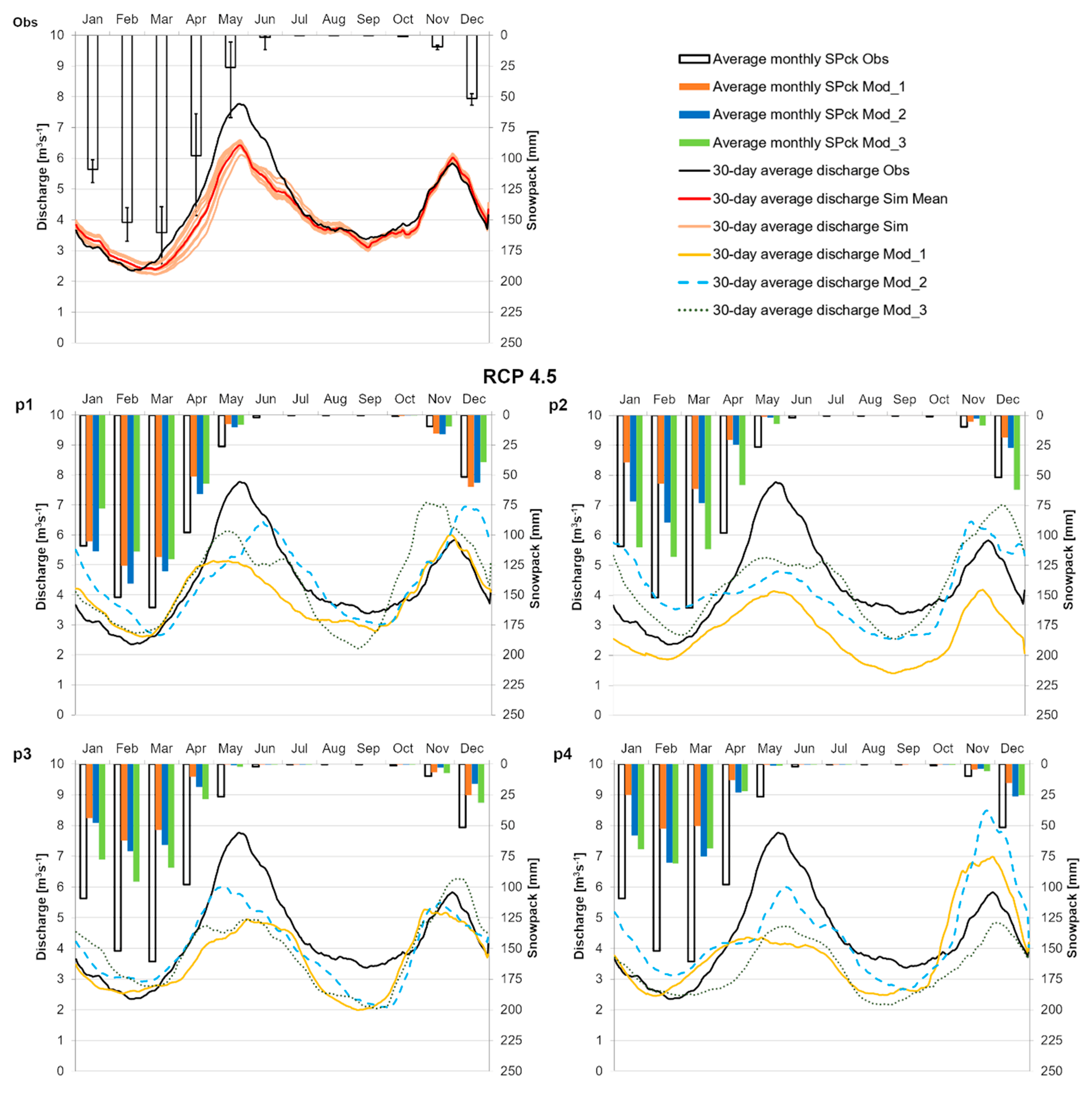
Figure 9 shows the relationships between the average snowpack thickness (expressed in snow water equivalent) and the 30-day average discharge in the Nossana basin, for the observation modelling period (2000–2017) and the four future periods under RCP 4.5. Under RCP 2.6 and RCP 8.5, the variables behave according to the same principles and thus they are not shown. First, Figure 9 shows that the model can reproduce the observed annual cycle of the 30-day discharge, with a slight underestimation of the peak occurring in May. The snowpack thickness is an output of the CemaNeige routine; no observed data are available, and so therefore it is possible that the snowpack thickness and the spring snowmelt are slightly underestimated. However, considering that April and May observed average precipitation is similar (Figure 5), the increase in the 30-day average discharge occurring during these two months is due to snowmelt. This dynamic is well represented by the model outputs. In future periods, the average thickness of the snowpack decreases with time, with similar relative paths in all months. Total precipitation in January, February, and March is not projected to decrease much (Figure 5), meaning that the relative future partitioning into rainfall and snow will favor the first. This reflects in 30-day discharges generally higher in all future intervals than during the observation period. Conversely, the 30-day discharge peak that used to occur in late May will be less pronounced and anticipated. In summer, the projected decreases in 30-day discharge are associated to both increasing temperature and decreasing precipitation (Figure 5). The 30-day discharge peaks projected for the autumn period (clearly evident in p1, p2, and p4) are mainly linked to increasing precipitation and only secondarily to increasing temperature, which affects precipitation partitioning. RCP 8.5 shows a similar annual trend in comparison to RCP 4.5 but average 30-day discharge during late spring and summer (May-September) are lower, up to an average of around 1.2 m3 s−1 (Mod_1 p4). In addition, in p4 the spring peak for Mod_1 disappears and similar average discharges occur from late January to mid-June. Conversely, the major difference between RCP 4.5 and RCP 2.6 is the absence, for the latter, of the discharge peak in autumn (related to an absence of precipitation peak, see Figure 4).
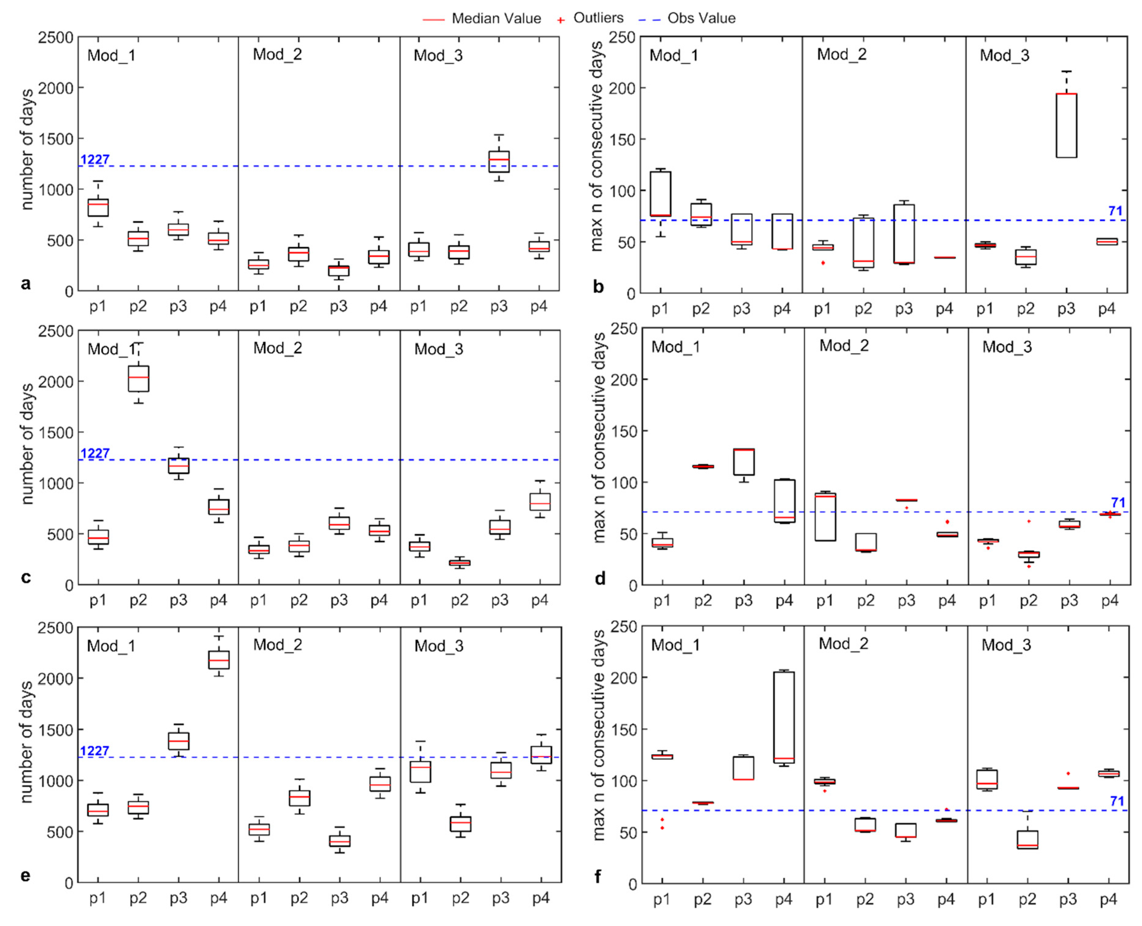
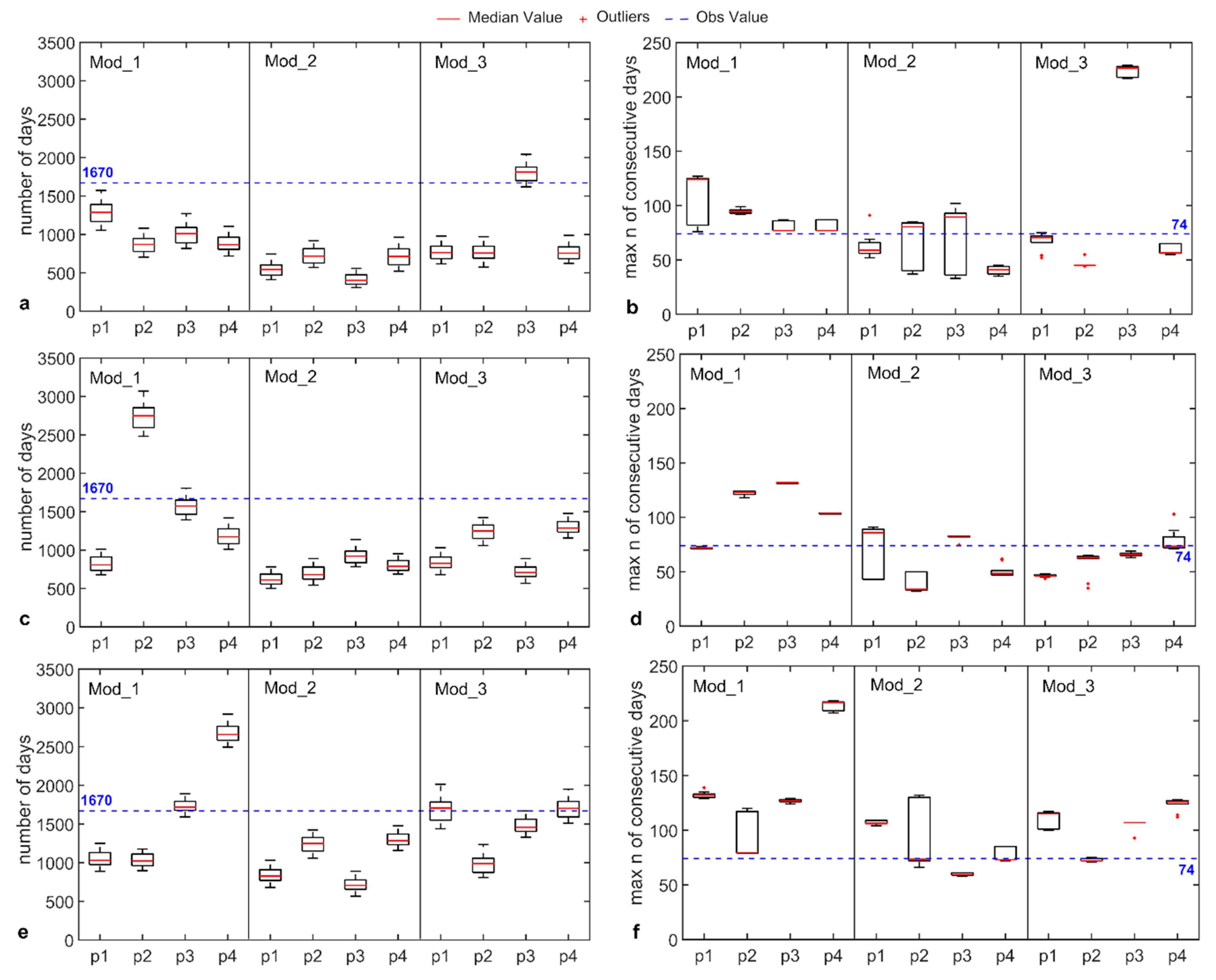
The boxplots in Figure 10 (Figure 11) show the distribution of the number of days and maximum number of consecutive days below the 1.32 m3 s−1 (1.52 m3 s−1) warning threshold for the rainfall-runoff model ensemble, presented by RCP scenario, RCM, and the twenty-year period. Variability within the rainfall-runoff ensemble appears larger for these indices rather than for the mean discharge. Especially for the consecutive number of days below the warning thresholds and dry period, single parameterizations lead to values with differences larger than 70% between each other.
In terms of ensemble mean, the number of days below the warning thresholds (both values) are projected to decrease in all cases, except for p4 under RCP8.5. Looking at single RCMs, there are few cases of simulations counting an increasing number of days below the warning thresholds, in comparison to observations, mainly related to Mod_1 and Mod_3 under RCP4.5 and RCP8.5. Under RCP2.6, only Mod_3 projects an increasing number of days below thresholds limited to p3.
Conversely, in terms of ensemble mean, the maximum number of consecutive days below the thresholds is projected to increase after 2060 for all emission scenarios (except p3, RCP2.6), although not all RCMs agree. The length of the longest period below the 1.32 m3 s−1 (1.52 m3 s−1) warning threshold can be as long as 36 (64) extra days. This trend is particularly evident for the 1.52 m3 s−1 warning threshold (Figure 11). However, this trend is particularly alarming for p4 since temperature is projected to increase from 1.0 °C to 5.8 °C (all RCPs and RCMs considered singularly), which will probably cause an increase in the water demand.
6. Discussion
Groppelli et al. [94,95] produced five future climate scenarios by statistical downscaling of three GCMs (2010–2060), forced under the A2 IPCC emission scenario [96], over the Oglio basin, the main valley east of the Seriana Valley. The A2 emission scenario, derived in the framework of 4th IPCC report [96], is somewhat comparable to RCP8.5, derived in the framework of the 5th IPCC report [2]. For the ten years around 2050 (in comparison to 1990–1999), they found an increase in mean annual temperature at 2000 m a.s.l. in the range 1.6–4.8 °C. At a lower elevation (around 600 m a.s.l.), for a comparable period (2041–2060) and scenario (RCP8.5), in this study a temperature increase in the range 1.8–2.8 °C was found. Larger increases could be expected only toward the end of the century (up to 5.8 °C). In terms of mean annual precipitation, Groppelli et al. [94,95] found variations between −15% and 40%, while in this study results suggest more limited changes (from −7% to 15%). The 18.5% decrease was obtained for the period 2041–2060, but under RCP4.5.
It is recognized that the selection of a rainfall-runoff modeling approach implies the assumption that the karst system will not undergo profound changes in the next 80 years, as pointed out by Hartmann et al. [16]. Specifically on the utilized rainfall-runoff model (GR4J with CemaNeige as snow accounting routing), it was found that the CemaNeige snow routine including hysteresis did not increase the performance of the model in terms of simulated discharge. This is in agreement with Riboust et al. [80], who found that accounting for hysteresis improved model simulations limited to snow cover area.
Gattinoni and Francani [60] calibrated a distributed equivalent porous media model (MODFLOW) for the simulation of Nossana Spring discharges and applied it to build spring depletion curves under variable recharge. The calibrated model and the depletion curves were then used to assess changes in spring behavior according to expected regional changes in temperature and precipitation, for the period 2080–2099 in comparison to 1980–1999, according to GCM forced under the A1B emission scenario [96]. All the models considered in their study suggested a decrease in mean annual precipitation (from 4% to 27%) and an increase in temperature (from 2.2 to 5.1 °C), which is in contrast with the results of this study obtained for the comparable RCP4.5 scenario (precipitation changes between −8% and 10%; temperature changes between 2.0 and 2.6 °C). However, due to the maximum expected precipitation decrease and evapotranspiration increase, they suggested a possible decrease in the spring discharge up to 40%, which is similar to the 39% decrease calculated in this study for the period 2041–2060 (Mod_2, see Figure 8b) for a precipitation decrease of 18.5% (Table 5) and a temperature increase of 2.1 °C. Gattinoni and Francani [60] also suggested that changes of the precipitation regime during the recharge season (March to November) are expected to have the largest influence on spring discharge. This is proven by the results of this study, which showed how the changes in precipitation partitioning between January and May will change the 30-day average discharge, anticipating and decreasing the observed late spring high flows. In addition, the projected rainfall decreases affecting the summer period (June to September) will reduce Nossana Spring discharges during this season. Higher recharge, in comparison to the recent past, can be expected in October, November, and December.
7. Conclusions
Climate change directly impacts the water cycle and consequently groundwater resources. Therefore, planning their management is essential for their protection and responsible use. In this study, a comprehensive methodological approach for the evaluation of future climate and discharge variations (up to 2100, in four twenty-year intervals) at Nossana karst spring was presented. The method is based on the statistical downscaling of three bias-corrected EURO-CORDEX RCMs forced by three different emission scenarios (RCP2.6, RCP4.5, RCP8.5) and the implementation of a rainfall-runoff model (GR4J) extended with a snow accounting routine (CemaNeige). Today, Nossana Spring is exploited by UniAcque S.p.A. for the supply of drinking water to 300,000 people (including the town of Bergamo). Simulated discharges were evaluated in terms of mean flow and in comparison to actual water demands (expressed as discharge warning thresholds), to provide projections that can be operationally useful to the service company.
Based on the presented results, the following can be concluded:
- The considered bias-corrected EURO-CORDEX RCMs have very good skills in reproducing observed temperature climatology (NSE > 0.95 and relative MAE < 10%) over the study area, while larger errors persist regarding precipitation (NSE between 0.25 and 0.65, relative MAE between 10% and 20%);
- According to the downscaled RCMs data, in comparison to 1998–2017, mean temperature will likely increase throughout the rest of the XXI century, from 0.7 °C in 2021–2040 (RCP4.5, Mod_2) to 5.8 °C in 2081–2100 (RCP8.5, Mod_1);
- Downscaled RCMs data do not show a clear trend in precipitation. For all twenty-year periods and RCP scenarios, there are single RCMs projecting increasing and decreasing rainfall (except 2021–2040, RCP2.6, all increasing). Variations in mean annual rainfall varies between −18.5% (2041–2060, RCP4.5, Mod_2) and 15.1% (2041–2060, RCP8.5, Mod_2);
- A pronounced decrease of precipitation is expected in the summer period after 2060, as most RCM-RCP combinations show;
- Mean discharges are generally projected to decrease in comparison to observed flow (3.77 m3 s−1) since changes in mean annual precipitation usually do not balance increases in evapotranspiration rates due to higher temperatures;
- Variability in the projected mean discharges is mainly linked to the meteorological input rather than the rainfall-runoff model parameterization;
- The maximum number of consecutive days below the warning thresholds was recognized as the best index to evaluate the spring low flow conditions;
- After 2060, the length of the periods with discharge lower than the warning thresholds is expected to increase. These periods could last up to 64 days (86%) longer than in 1998–2017.
The present study indicates that additional water resources might be needed to satisfy the population water demand in the Nossana Spring area, especially after 2060. Therefore, the presented approach can be considered useful to provide indications regarding the management of the resource in the mid- long-term period. In fact, UniAcque S.p.A. will soon start to investigate possible alternative sources for water supply. However, it is evident that the results include large uncertainties derived from the climate input variability, especially precipitation, and as new emission scenarios are produced, the study should be updated.
Furthermore, the study focused on the quantitative aspects of the spring behavior; however, it is possible that a change in the discharge regime could also influence the chemical-physical characteristics of the water and its quality. A chemical-isotopic monitoring of the spring could improve the conceptual model of the aquifer system and the knowledge of the system response. This would allow a refinement of the method, raising it to a qualitative and quantitative prevision of the resource behavior.
Author Contributions
Conceptualization, A.C., C.C. and G.P.B.; methodology, A.C., C.C; software, A.C., C.C.; formal analysis, A.C.; investigation, A.C., C.C.; resources, G.P.B.; data curation, A.C.; writing—original draft preparation, A.C.; writing—review and editing, C.C, G.P.B.; supervision, C.C., G.P.B.; funding acquisition, G.P.B. All authors have read and agreed to the published version of the manuscript.
Funding
This research was jointly funded by the framework agreement between UniAcque S.p.A. and Dipartimento di Scienze della Terra “Ardito Desio” and the Italian Ministry of Education (MIUR) through the project “Dipartimenti di Eccellenza 2017”.
Acknowledgments
Authors wish to thank Georgios Zittis, for his help and suggestions in the selection and processing of the EURO-CORDEX data, and Daniele Pedretti, for support with the language proofreading. In addition, authors would like to acknowledge the two anonymous reviewers, whose comments have contributed to increasing the quality of this manuscript.
Conflicts of Interest
The authors declare no conflict of interest.
References
- Bakalowicz, M. Karst groundwater: A challenge for new resources. Hydrogeol. J. 2005, 13, 148–160. [Google Scholar] [CrossRef]
- Core Writing Team; Pachauri, R.K.; Meyer, L.A. (Eds.) IPCC Climate Change 2014: Synthesis Report. Contribution of Working Groups I, II and III to the Fifth Assessment Report of the Intergovernmental Panel on Climate Change; IPCC: Geneva, Switzerland, 2014; p. 151. [Google Scholar]
- Liesch, T.; Wunsch, A. Aquifer responses to long-term climatic periodicities. J. Hydrol. 2019, 572, 226–242. [Google Scholar] [CrossRef]
- Kløve, B.; Ala-Aho, P.; Bertrand, G.; Gurdak, J.J.; Kupfersberger, H.; Kværner, J.; Muotka, T.; Mykrä, H.; Preda, E.; Rossi, P.; et al. Climate change impacts on groundwater and dependent ecosystems. J. Hydrol. 2014, 518, 250–266. [Google Scholar] [CrossRef]
- Pedretti, D.; Russian, A.; Sanchez-Vila, X.; Dentz, M. Scale dependence of the hydraulic properties of a fractured aquifer estimated using transfer functions. Water Resour. Res. 2016, 52, 5008–5024. [Google Scholar] [CrossRef] [Green Version]
- Scanlon, B.R.; Mace, E.R.; Barrett, E.M.; Smith, B. Can we simulate regional groundwater flow in a karst system using equivalent porous media models? Case study, Barton Springs Edwards aquifer, USA. J. Hydrol. 2003, 276, 137–158. [Google Scholar] [CrossRef]
- Worthington, S.R.H. Diagnostic hydrogeologic characteristics of a karst aquifer (Kentucky, USA). Hydrogeol. J. 2009, 17, 1665–1678. [Google Scholar] [CrossRef]
- Ford, D.; Williams, P. Karst Hydrogeology and Geomorphology; Wiley: Hoboken, NJ, USA, 2007. [Google Scholar]
- Zhang, B.; Lerner, D.N. Modeling of Ground Water Flow to Adits. Ground Water 2000, 38, 99–105. [Google Scholar] [CrossRef]
- Bauer, S.; Liedl, R.; Sauter, M. Modeling of karst aquifer genesis: Influence of exchange flow. Water Resour. Res. 2003, 39. [Google Scholar] [CrossRef]
- Liedl, R.; Hückinghaus, D.; Clemens, T.; Sauter, M.; Teutsch, G. Simulation of the development of karst aquifers using a coupled continuum pipe flow model. Water Resour. Res. 2003, 39. [Google Scholar] [CrossRef]
- Shoemaker, W.B.; Kuniansky, E.L.; Birk, S.; Bauer, S.; Swain, E.D. Documentation of a conduit flow process (CFP) for MODFLOW-2005Techniques and Methods. In U.S. Geologist Survival Technology Methods; U.S. Geological Survey: Reston, VA, USA, 2008; Book 6; 50p. [Google Scholar]
- Reimann, T.; Geyer, T.; Shoemaker, W.B.; Liedl, R.; Sauter, M. Effects of dynamically variable saturation and matrix-conduit coupling of flow in karst aquifers. Water Resour. Res. 2011, 47. [Google Scholar] [CrossRef]
- De Rooij, R.; Perrochet, P.; Graham, W. From rainfall to spring discharge: Coupling conduit flow, subsurface matrix flow and surface flow in karst systems using a discrete–continuum model. Adv. Water Resour. 2013, 61, 29–41. [Google Scholar] [CrossRef]
- Chang, Y.; Wu, J.; Jiang, G.; Liu, L.; Reimann, T.; Sauter, M. Modelling spring discharge and solute transport in conduits by coupling CFPv2 to an epikarst reservoir for a karst aquifer. J. Hydrol. 2019, 569, 587–599. [Google Scholar] [CrossRef]
- Hartmann, A.; Goldscheider, N.; Wagener, T.; Lange, J.; Weiler, M. Karst water resources in a changing world: Review of hydrological modeling approaches. Rev. Geophys. 2014, 52, 218–242. [Google Scholar] [CrossRef]
- Prelovšek, M.; Turk, J.; Gabrovšek, F. Hydrodynamic aspect of caves. Int. J. Speleol. 2008, 37, 11–26. [Google Scholar] [CrossRef]
- Goldscheider, N.; Meiman, J.; Pronk, M.; Smart, C. Tracer tests in karst hydrogeology and speleology. Int. J. Speleol. 2008, 37, 27–40. [Google Scholar] [CrossRef] [Green Version]
- Aquilina, L.; Ladouche, B.; Dörfliger, N. Water storage and transfer in the epikarst of karstic systems during high flow periods. J. Hydrol. 2006, 327, 472–485. [Google Scholar] [CrossRef]
- Barberá, J.A.; Andreo, B. Functioning of a karst aquifer from S Spain under highly variable climate conditions, deduced from hydrochemical records. Environ. Earth Sci. 2012, 65, 2337–2349. [Google Scholar] [CrossRef]
- Erőss, A.; Mádl-Szőnyi, J.; Surbeck, H.; Horváth, Á.; Goldscheider, N.; Csoma, A.É. Radionuclides as natural tracers for the characterization of fluids in regional discharge areas, Buda Thermal Karst, Hungary. J. Hydrol. 2012, 426, 124–137. [Google Scholar]
- Binet, S.; Joigneaux, E.; Pauwels, H.; Albéric, P.; Fléhoc, C.; Bruand, A. Water exchange, mixing and transient storage between a saturated karstic conduit and the surrounding aquifer: Groundwater flow modeling and inputs from stable water isotopes. J. Hydrol. 2017, 544, 278–289. [Google Scholar] [CrossRef] [Green Version]
- Brkić, Ž.; Kuhta, M.; Hunjak, T. Groundwater flow mechanism in the well-developed karst aquifer system in the western Croatia: Insights from spring discharge and water isotopes. Catena 2018, 161, 14–26. [Google Scholar] [CrossRef]
- Mace, R.E. Determination of Transmissivity from Specific Capacity Tests in a Karst Aquifer. Ground Water 1997, 35, 738–742. [Google Scholar] [CrossRef]
- Kresic, N. Hydraulic methods. In Methods in Karst Hydrogeology; Taylor and Francis/Balkema: London, UK, 2014; pp. 65–91. [Google Scholar]
- Šumanovac, F.; Weisser, M. Evaluation of resistivity and seismic methods for hydrogeological mapping in karst terrains. J. Appl. Geophys. 2001, 47, 13–28. [Google Scholar] [CrossRef]
- Andrade-Gómez, L.; Rebolledo-Vieyra, M.; Andrade, J.L.; López, P.Z.; Estrada-Contreras, J. Karstic aquifer structure from geoelectrical modeling in the Ring of Sinkholes, Mexico. Hydrogeol. J. 2019, 27, 2365–2376. [Google Scholar] [CrossRef]
- Kaufmann, G. Geophysical mapping of solution and collapse sinkholes. J. Appl. Geophys. 2014, 111, 271–288. [Google Scholar] [CrossRef]
- Jardani, A.; Revil, A.; Dupont, J.P. Self-potential tomography applied to the determination of cavities. Geophys. Res. Lett. 2006, 33. [Google Scholar] [CrossRef]
- Fleury, P.; Plagnes, V.; Bakalowicz, M. Modelling of the functioning of karst aquifers with a reservoir model: Application to Fontaine de Vaucluse (South of France). J. Hydrol. 2007, 345, 38–49. [Google Scholar] [CrossRef]
- Mazzilli, N.; Guinot, V.; Jourde, H.; Lecoq, N.; Labat, D.; Arfib, B.; Baudement, C.; Danquigny, C.; Soglio, L.D.; Bertin, D. KarstMod: A modelling platform for rainfall-discharge analysis and modelling dedicated to karst systems. Environ. Model. Softw. 2019, 122. [Google Scholar] [CrossRef] [Green Version]
- Kurtulus, B.; Razack, M. Modeling daily discharge responses of a large karstic aquifer using soft computing methods: Artificial neural network and neuro-fuzzy. J. Hydrol. 2010, 381, 101–111. [Google Scholar] [CrossRef]
- Denić-Jukić, V.; Jukić, D. Composite transfer functions for karst aquifers. J. Hydrol. 2003, 274, 80–94. [Google Scholar] [CrossRef]
- Long, A.J. RRAWFLOW: Rainfall-Response Aquifer and Watershed Flow Model (v1.15). Geosci. Model Dev. 2015, 8, 865–880. [Google Scholar] [CrossRef] [Green Version]
- Mudarra, M.; Hartmann, A.; Andreo, B. Combining Experimental Methods and Modeling to Quantify the Complex Recharge Behavior of Karst Aquifers. Water Resour. Res. 2019, 55, 1384–1404. [Google Scholar] [CrossRef]
- Sapač, K.; Medved, A.; Rusjan, S.; Bezak, N. Investigation of Low- and High-Flow Characteristics of Karst Catchments under Climate Change. Water 2019, 11, 925. [Google Scholar] [CrossRef] [Green Version]
- Sappa, G.; De Filippi, F.M.; Iacurto, S.; Grelle, G. Evaluation of Minimum Karst Spring Discharge Using a Simple Rainfall-Input Model: The Case Study of Capodacqua di Spigno Spring (Central Italy). Water 2019, 11, 807. [Google Scholar] [CrossRef] [Green Version]
- Sezen, C.; Bezak, N.; Bai, Y.; Šraj, M. Hydrological modelling of karst catchment using lumped conceptual and data mining models. J. Hydrol. 2019, 576, 98–110. [Google Scholar] [CrossRef]
- Sivelle, V.; Labat, D.; Mazzilli, N.; Massei, N.; Jourde, H. Dynamics of the Flow Exchanges between Matrix and Conduits in Karstified Watersheds at Multiple Temporal Scales. Water 2019, 11, 569. [Google Scholar] [CrossRef] [Green Version]
- Klemeš, V. Operational testing of hydrological simulation models. Hydrol. Sci. J. 1986, 31, 13–24. [Google Scholar] [CrossRef]
- Kuczera, G.; Mroczkowski, M. Assessment of hydrologic parameter uncertainty and the worth of multiresponse data. Water Resour. Res. 1998, 34, 1481–1489. [Google Scholar] [CrossRef]
- Vaze, J.; Post, D.; Chiew, F.; Perraud, J.-M.; Viney, N.; Teng, J. Climate non-stationarity—Validity of calibrated rainfall–runoff models for use in climate change studies. J. Hydrol. 2010, 394, 447–457. [Google Scholar] [CrossRef]
- Coron, L.; Andréassian, V.; Perrin, C.; Lerat, J.; Vaze, J.; Bourqui, M.; Hendrickx, F. Crash testing hydrological models in contrasted climate conditions: An experiment on 216 Australian catchments. Water Resour. Res. 2012, 48. [Google Scholar] [CrossRef] [Green Version]
- Le Coz, M.; Bruggeman, A.; Camera, C.; Lange, M.A. Impact of precipitation variability on the performance of a rainfall–runoff model in Mediterranean mountain catchments. Hydrol. Sci. J. 2016, 61, 507–518. [Google Scholar] [CrossRef] [Green Version]
- Meinshausen, M.; Smith, S.J.; Calvin, K.; Daniel, J.S.; Kainuma, M.L.T.; Lamarque, J.-F.; Matsumoto, K.; Montzka, S.A.; Raper, S.C.B.; Riahi, K.; et al. The RCP greenhouse gas concentrations and their extensions from 1765 to 2300. Clim. Chang. 2011, 109, 213. [Google Scholar] [CrossRef] [Green Version]
- Kreienkamp, F.; Paxian, A.; Früh, B.; Lorenz, P.; Matulla, C. Evaluation of the empirical–statistical downscaling method EPISODES. Clim. Dyn. 2019, 52, 991–1026. [Google Scholar] [CrossRef] [Green Version]
- Rummukainen, M. State-of-the-art with regional climate models. WIREs Clim. Chang. 2010, 1, 82–96. [Google Scholar] [CrossRef]
- Kotlarski, S.; Keuler, K.; Christensen, O.B.; Colette, A.; Déqué, M.; Gobiet, A.; Goergen, K.; Jacob, D.; Lüthi, D.; van Meijgaard, E.; et al. Regional climate modeling on European scales: A joint standard evaluation of the EURO-CORDEX RCM ensemble. Geosci. Model Dev. 2014, 7, 1297–1333. [Google Scholar] [CrossRef] [Green Version]
- Zittis, G.; Bruggeman, A.; Camera, C.; Hadjinicolaou, P.; Lelieveld, J. The added value of convection permitting simulations of extreme precipitation events over the eastern Mediterranean. Atmospheric Res. 2017, 191, 20–33. [Google Scholar] [CrossRef]
- Adhikari, A.; Hansen, A.J.; Rangwala, I. Ecological Water Stress under Projected Climate Change across Hydroclimate Gradients in the North-Central United States. J. Appl. Meteorol. Clim. 2019, 58, 2103–2114. [Google Scholar] [CrossRef]
- Haslinger, K.; Anders, I.; Hofstätter, M. Regional climate modelling over complex terrain: An evaluation study of COSMO-CLM hindcast model runs for the Greater Alpine Region. Clim. Dyn. 2013, 40, 511–529. [Google Scholar] [CrossRef]
- Benestad, R.E.; Hanssen-Bauer, I.; Chen, D. Empirical-Statistical Downscaling; World Scientific Publishing Company: Hoboken, NJ, USA; London, UK, 2008; ISBN 978-981-281-912-3. [Google Scholar]
- Piani, C.; Haerter, J.O.; Coppola, E. Statistical bias correction for daily precipitation in regional climate models over Europe. Theor. Appl. Climatol. 2010, 99, 187–192. [Google Scholar] [CrossRef] [Green Version]
- Gutiérrez, J.M.; San-Martín, D.; Brands, S.; Manzanas, R.; Herrera, S. Reassessing Statistical Downscaling Techniques for Their Robust Application under Climate Change Conditions. J. Clim. 2012, 26, 171–188. [Google Scholar] [CrossRef] [Green Version]
- Maraun, D.; Wetterhall, F.; Ireson, A.M.; Chandler, R.E.; Kendon, E.J.; Widmann, M.; Brienen, S.; Rust, H.W.; Sauter, T.; Themeßl, M.; et al. Precipitation downscaling under climate change: Recent developments to bridge the gap between dynamical models and the end user. Rev. Geophys. 2010, 48. [Google Scholar] [CrossRef]
- Perrin, C.; Michel, C.; Andréassian, V. Improvement of a parsimonious model for streamflow simulation. J. Hydrol. 2003, 279, 275–289. [Google Scholar] [CrossRef]
- Valéry, A.; Andréassian, V.; Perrin, C. ‘As simple as possible but not simpler’: What is useful in a temperature-based snow-accounting routine? Part 1—Comparison of six snow accounting routines on 380 catchments. J. Hydrol. 2014, 517, 1166–1175. [Google Scholar] [CrossRef]
- Valéry, A.; Andréassian, V.; Perrin, C. ‘As simple as possible but not simpler’: What is useful in a temperature-based snow-accounting routine? Part 2—Sensitivity analysis of the Cemaneige snow accounting routine on 380 catchments. J. Hydrol. 2014, 517, 1176–1187. [Google Scholar] [CrossRef]
- Chardon, M. La moyenne vallée du Serio: Étude morphologique. Méditerranée 1974, 17, 43–62. [Google Scholar] [CrossRef]
- Gattinoni, P.; Francani, V. Depletion risk assessment of the Nossana Spring (Bergamo, Italy) based on the stochastic modeling of recharge. Hydrogeol. J. 2010, 18, 325–337. [Google Scholar] [CrossRef]
- Curioni, G. Geologia: Geologia Applicata Delle Provincie Lombarde; U. Hoepli: Milan, Italy, 1877. [Google Scholar]
- Desio, A. Sull’origine della sorgente di Nossa e sulla tettonica dei dintorni. Atti Della Soc. Ital. Di Sci. Nat. 1943, 82, 141–150. [Google Scholar]
- Forcella, F.; Jadoul, F. Carta Geologica Della Provincia Di Bergamo Alla Scala 1:50.000 Con Relativa Nota Illustrativa; Assessorato all’Ambiente della Provincia di Bergamo: Bergamo, Italy, 2000; 313p. [Google Scholar]
- Zanchi, A.; D’Adda, P.; Zanchetta, S.; Berra, F. Syn-thrust deformation across a transverse zone: The Grem–Vedra fault system (central Southern Alps, N Italy). Swiss J. Geosci. 2012, 105, 19–38. [Google Scholar] [CrossRef]
- Jadoul, F.; Pozzi, R.; Pestrin, S. La sorgente Nossana: Inquadramento geologico e idrogeologico (Val Seriana, prealpi bergamasche). Riv. Mus. Civ. Sci. Nat. 1985, 9, 129–140. [Google Scholar]
- Jadoul, F.; Berra, F.; Bini, A.; Ferliga, C.; Mazzoccola, D.; Papani, L.; Piccin, A.; Rossi, R.; Rossi, S.; Trombetta, G.L. Note illustrative della carta geologica d’Italia alla scala 1:50.000. Foglio 077—Clusone; ISPRA: Rome, Italy, 2012. [Google Scholar]
- Vigna, B.; Banzato, C. The hydrogeology of high-mountain carbonate areas: An example of some Alpine systems in southern Piedmont (Italy). Environ. Earth Sci. 2015, 74, 267–280. [Google Scholar] [CrossRef]
- Peel, M.C.; Finlayson, B.L.; McMahon, T.A. Updated world map of the Köppen-Geiger climate classification. Hydrol. Earth Syst. Sci. 2007, 11, 1633–1644. [Google Scholar] [CrossRef] [Green Version]
- Yang, W.; Andréasson, J.; Graham, L.P.; Olsson, J.; Rosberg, J.; Wetterhall, F. Distribution-based scaling to improve usability of regional climate model projections for hydrological climate change impacts studies. Hydrol. Res. 2010, 41, 211–229. [Google Scholar] [CrossRef]
- Nash, J.E.; Sutcliffe, J.V. River Flow forecasting through conceptual models-Part I: A discussion of principles. J. Hydrol. 1970, 10, 282–290. [Google Scholar] [CrossRef]
- Camera, C.; Bruggeman, A.; Hadjinicolaou, P.; Michaelides, S.; Lange, M.A. Evaluation of a spatial rainfall generator for generating high resolution precipitation projections over orographically complex terrain. Stoch. Environ. Res. Risk Assess. 2017, 31, 757–773. [Google Scholar] [CrossRef]
- Prudhomme, C.; Reynard, N.; Crooks, S. Downscaling of global climate models for flood frequency analysis: Where are we now? Hydrol. Process. 2002, 16, 1137–1150. [Google Scholar] [CrossRef]
- Kilsby, C.; Jones, P.; Burton, A.; Ford, A.; Fowler, H.; Harpham, C.; James, P.; Smith, A.; Wilby, R. A daily weather generator for use in climate change studies. Environ. Model. Softw. 2007, 22, 1705–1719. [Google Scholar] [CrossRef]
- Burton, A.; Kilsby, C.; Fowler, H.; Cowpertwait, P.; O’Connell, P. RainSim: A spatial–temporal stochastic rainfall modelling system. Environ. Model. Softw. 2008, 23, 1356–1369. [Google Scholar] [CrossRef]
- Rodriguez-Iturbe, I.; Cox, D.R.; Isham, V. Some Models for Rainfall Based on Stochastic Point Processes. Proc. R. Soc. A Math. Phys. Eng. Sci. 1987, 410, 269–288. [Google Scholar]
- Cowpertwait, P.S.P.; Kilsby, C.G.; O’Connell, P.E. A space-time Neyman-Scott model of rainfall: Empirical analysis of extremes. Water Resour. Res. 2002, 38. [Google Scholar] [CrossRef]
- Richardson, C.W. Stochastic simulation of daily precipitation, temperature, and solar radiation. Water Resour. Res. 1981, 17, 182–190. [Google Scholar] [CrossRef]
- Camera, C.; Bruggeman, A.; Hadjinicolaou, P.; Pashiardis, S.; Lange, M.A. High Resolution Gridded Datasets for Meteorological Variables: Cyprus, 1980–2010 and 2020–2050; AGWATER Scientific Report 5; The Cyprus Institute: Nicosia, Cyprus, 2013; p. 77. [Google Scholar]
- Matalas, N.C. Mathematical assessment of synthetic hydrology. Water Resour. Res. 1967, 3, 937–945. [Google Scholar] [CrossRef]
- Riboust, P.; Thirel, G.; Le Moine, N.; Ribstein, P. Revisiting a Simple Degree-Day Model for Integrating Satellite Data: Implementation of Swe-Sca Hystereses. J. Hydrol. Hydromechanics 2019, 67, 70–81. [Google Scholar] [CrossRef] [Green Version]
- Coron, L.; Thirel, G.; Delaigue, O.; Perrin, C.; Andréassian, V. The suite of lumped GR hydrological models in an R package. Environ. Model. Softw. 2017, 94, 166–171. [Google Scholar] [CrossRef]
- Coron, L.; Delaigue, O.; Thirel, G.; Perrin, C.; Michel, C. airGR: Suite of GR Hydrological Models for Precipitation-Runoff Modelling (2019). Available online: https://CRAN.R-project.org/package=airGR (accessed on 25 June 2019).
- Le Moine, N.; Andréassian, V.; Perrin, C.; Michel, C. How can rainfall-runoff models handle intercatchment groundwater flows? Theoretical study based on 1040 French catchments. Water Resour. Res. 2007, 43. [Google Scholar] [CrossRef]
- Pushpalatha, R.; Perrin, C.; Le Moine, N.; Mathevet, T.; Andréassian, V. A downward structural sensitivity analysis of hydrological models to improve low-flow simulation. J. Hydrol. 2011, 411, 66–76. [Google Scholar] [CrossRef]
- Guinot, V.; Savéan, M.; Jourde, H.; Neppel, L. Conceptual rainfall-runoff model with a two-parameter, infinite characteristic time transfer function. Hydrol. Process. 2015, 29, 4756–4778. [Google Scholar] [CrossRef] [Green Version]
- Moussu, F.; Oudin, L.; Plagnes, V.; Mangin, A.; Bendjoudi, H. A multi-objective calibration framework for rainfall–discharge models applied to karst systems. J. Hydrol. 2011, 400, 364–376. [Google Scholar] [CrossRef]
- Hargreaves, G.H.; Samani, Z.A. Reference Crop Evapotranspiration from Temperature. Appl. Eng. Agric. 1985, 1, 96–99. [Google Scholar] [CrossRef]
- Consiglio Superiore Servizio Idrografico. Carta Della Precipitazione Nevosa Media Annua in Italia Nel Quarantennio 1921–1960; Ministero dei Lavori Pubblici: Rome, Italy, 1972.
- Centro Meteorologico Lombardo. Atlante Dei Climi E Dei Microclimi Della Lombardia; Grafica Sette: Brescia, Italy, 2011; 352p. [Google Scholar]
- Senese, A.; Maugeri, M.; Meraldi, E.; Verza, G.P.; Azzoni, R.S.; Compostella, C.; Diolaiuti, G. Estimating the snow water equivalent on a glacierized high elevation site (Forni Glacier, Italy). Cryosphere 2018, 12, 1293–1306. [Google Scholar] [CrossRef] [Green Version]
- Ayzel, G.; Varentsova, N.; Erina, O.; Sokolov, D.; Kurochkina, L.; Moreydo, V. OpenForecast: The First Open-Source Operational Runoff Forecasting System in Russia. Water 2019, 11, 1546. [Google Scholar] [CrossRef] [Green Version]
- Gupta, H.V.; Kling, H.; Yilmaz, K.K.; Martinez, G.F. Decomposition of the mean squared error and NSE performance criteria: Implications for improving hydrological modelling. J. Hydrol. 2009, 377, 80–91. [Google Scholar] [CrossRef] [Green Version]
- Kling, H.; Fuchs, M.; Paulin, M. Runoff conditions in the upper Danube basin under an ensemble of climate change scenarios. J. Hydrol. 2012, 424, 264–277. [Google Scholar] [CrossRef]
- Groppelli, B.; Bocchiola, D.; Rosso, R. Spatial downscaling of precipitation from GCMs for climate change projections using random cascades: A case study in Italy. Water Resour. Res. 2011, 47. [Google Scholar] [CrossRef]
- Groppelli, B.; Soncini, A.; Bocchiola, D.; Rosso, R. Evaluation of future hydrological cycle under climate change scenarios in a mesoscale Alpine watershed of Italy. Nat. Hazards Earth Syst. Sci. 2011, 11, 1769–1785. [Google Scholar] [CrossRef] [Green Version]
- Nakicenovic, N.; Swart, R.E. (Eds.) IPCC Emission Scenarios, a Special Report of Working Group III of the Intergovernmental Panel on Climate Change; Cambridge University Press: Cambridge, UK, 2000; p. 570. [Google Scholar]
Figure 1.
Geographical and geological setting of the study area.

Figure 2.
Flow chart summarizing the applied methodological approach.

Figure 3.
Schematic representation of the coupling between the GR4J hydrological model and the Cema-Neige snow accounting routine.
Figure 3.
Schematic representation of the coupling between the GR4J hydrological model and the Cema-Neige snow accounting routine.

Figure 4.
Comparison between the observed and projected monthly climatology for the three RCMs (Mod_1, Mod_2 and Mod_3, see Table 1) forced under RCP 2.6 for four twenty-year periods p1 is 2021−2040, p2 is 2041−2060, p3 is 2061−2080, and p4 is 2081−2100.
Figure 4.
Comparison between the observed and projected monthly climatology for the three RCMs (Mod_1, Mod_2 and Mod_3, see Table 1) forced under RCP 2.6 for four twenty-year periods p1 is 2021−2040, p2 is 2041−2060, p3 is 2061−2080, and p4 is 2081−2100.

Figure 5.
Comparison between the observed and projected monthly climatology for the three RCMs (Mod_1, Mod_2 and Mod_3, see Table 1) forced under RCP 4.5 for four twenty-year periods; p1 is 2021−2040, p2 is 2041−2060, p3 is 2061−2080, and p4 is 2081−2100.
Figure 5.
Comparison between the observed and projected monthly climatology for the three RCMs (Mod_1, Mod_2 and Mod_3, see Table 1) forced under RCP 4.5 for four twenty-year periods; p1 is 2021−2040, p2 is 2041−2060, p3 is 2061−2080, and p4 is 2081−2100.

Figure 6.
Comparison between the observed and projected monthly climatology for the three RCMs (Mod_1, Mod_2 and Mod_3, see Table 1) forced under RCP 8.5 for four twenty-year periods; p1 is 2021−2040, p2 is 2041−2060, p3 is 2061−2080, and p4 is 2081−2100.
Figure 6.
Comparison between the observed and projected monthly climatology for the three RCMs (Mod_1, Mod_2 and Mod_3, see Table 1) forced under RCP 8.5 for four twenty-year periods; p1 is 2021−2040, p2 is 2041−2060, p3 is 2061−2080, and p4 is 2081−2100.

Figure 7.
Comparison between observed and simulated (a) daily discharges for the period 1998–2017, (b) non-exceedance probabilities of daily flow rates for the calibration period (2000–2008), and (c) the validation period (2009–2017). In (b) and (c) daily flow rates are plotted on a logarithmic scale.

Figure 8.
Boxplots representing the distribution of the mean daily discharge values obtained from the rainfall-runoff ensemble when run with time series obtained from different RCMs (Mod_1, Mod_2, Mod_3, see Table 1) for four twenty-year periods (p1, 2021–2040; p2, 2041–2060; p3, 2061–2080; and p4, 2081–2100) under different emission scenarios (a) RCP2.6, (b) RCP4.5 and (c) RCP8.5.The 3.77 m3 s−1 line represents the observed (1998–2017) mean daily discharge.

Figure 9.
Average monthly snowpack thickness (SPck, in snow water equivalent) and 30-day average discharge for the observation modelling period (Obs, 2000–2017) and four future time intervals (p1, 2021–2040; p2, 2041–2060; p3, 2061–2080; and p4, 2081–2100) under RCP4.5. Error bars indicate minimum and maximum values as simulated by the ensemble members. Mod_1, Mod_2, and Mod_3 refer to outputs related to three different RCMs (see Table 1).

Figure 10.
Boxplots representing the distribution of the number of days (left) and maximum number of consecutive days (right) below the 1.32 m3 s−1 warning threshold obtained from the rainfall-runoff ensemble when run with time series obtained from different RCMs (Mod_1, Mod_2, Mod_3, see Table 1), for four twenty-year periods (p1, 2021–2040; p2, 2041–2060; p3, 2061–2080; and p4, 2081-2100), under different emission scenarios a, b) RCP2.6, c, d) RCP4.5 and e, f) RCP8.5. The 1227 and 71 lines represent the observed (1998–2017) values.

Figure 11.
Boxplots representing the distribution of the number of days (left) and maximum number of consecutive days (right) below the 1.52 m3 s−1 warning threshold obtained from the rainfall-runoff ensemble when run with time series obtained from different RCMs (Mod_1, Mod_2, Mod_3, see Table 1), for four twenty-year periods (p1, 2021–2040; p2, 2041–2060; p3, 2061–2080; and p4, 2081–2100), under different emission scenarios a, b) RCP2.6, c, d) RCP4.5 and e, f) RCP8.5. The 1670 and 74 lines represent the observed (1998–2017) values.


Table 1.
Summary of the climate model data sources used for this study.
| ID | Global Circulation Model | Ensemble Member | Regional Climate Model | Institution |
|---|---|---|---|---|
| Mod_1 | ICHEC-EC-EARTH | r12i1p1 | RCA4_v1 | Swedish Meteorological and Hydrological Institute (SMHI) |
| Mod_2 | MPI-ESM-LR | r2i1p1 | REMO2009_v1 | Max Planck Institute for Meteorology, Climate Service Center |
| Mod_3 | MPI-ESM-LR | r1i1p1 | REMO2009_v1 | Max Planck Institute for Meteorology, Climate Service Center |
Table 2.
RainSim parameters for time series generation in single site mode [74].
Table 2.
RainSim parameters for time series generation in single site mode [74].
| Parameter | Description | Units |
|---|---|---|
| λ−1 | Mean time between adjacent storm origins | [h] |
| β−1 | Mean waiting time for raincell origins after storm origin | [h] |
| η−1 | Mean duration of raincell | [h] |
| Ν | Mean number of raincells per storm | [-] |
| ξ−1 | Mean intensity of a raincell | [mm·h−1] |
Table 3.
Parameter ranges used to generate the random samples for model calibration and validation.
| GR4J | ||
|---|---|---|
| Parameter | Description | Calibration Range |
| X1 | Production store capacity [mm] | 100–1200 |
| X2 | Intercatchment exchange coefficient [mm/day] | −5–3 |
| X3 | Routing store capacity (mm) | 20–300 |
| X4 | Time constant of unit hydrograph (day) | 1.1–2.9 |
| CemaNeige | ||
| X5-Kf | Weighting coefficient of the snowpack thermal state [-] | 0–1 |
| X6-Ctg | Day-degree rate of melting [mm °C−1 day−1] | 0–10 |
| X7-Tacc | Accumulation threshold [mm] | 0–45 |
| X8-Tmelt | Fraction of annual snowfall defining the melt threshold [-] | 0–1 |
Table 4.
Performance statistics for the considered RCMs calculated in comparison with observed precipitation, minimum temperature, and maximum temperature monthly climatology. NSE is the Nash –Sutcliffe Efficiency coefficient, MAE the Mean Absolute Error and %MAE the normalized Mean Absolute Error. For RCMs name attribution, the reader can refer to Table 1.
| Precipitation | Tmin | Tmax | |||||||
|---|---|---|---|---|---|---|---|---|---|
| Model | NSE | MAE (mm) | %MAE | NSE | MAE (°C) | %MAE | NSE | MAE (°C) | %MAE |
| Mod_1 RCP 2.6 | 0.79 | 12.35 | 10.71 | 0.96 | 1.10 | 17.69 | 0.97 | 1.18 | 7.09 |
| Mod_1 RCP 4.5 | 0.66 | 14.97 | 12.97 | 0.97 | 1.00 | 17.19 | 0.97 | 1.08 | 6.48 |
| Mod_1 RCP 8.5 | 0.76 | 12.71 | 11.20 | 0.97 | 1.00 | 15.96 | 0.98 | 0.90 | 5.43 |
| Mod_2 RCP 2.6 | 0.31 | 19.81 | 17.16 | 0.97 | 0.90 | 14.20 | 0.97 | 0.99 | 5.95 |
| Mod_2 RCP 4.5 | 0.52 | 17.44 | 15.12 | 0.97 | 1.00 | 16.13 | 0.96 | 1.27 | 7.65 |
| Mod_2 RCP 8.5 | 0.31 | 22.90 | 19.85 | 0.97 | 0.90 | 15.42 | 0.96 | 1.28 | 7.66 |
| Mod_3 RCP 2.6 | 0.23 | 20.53 | 17.79 | 0.97 | 1.00 | 15.96 | 0.96 | 1.19 | 7.14 |
| Mod_3 RCP 4.5 | 0.37 | 17.17 | 14.88 | 0.98 | 0.80 | 12.79 | 0.97 | 0.99 | 5.95 |
| Mod_3 RCP 8.5 | 0.52 | 17.78 | 15.41 | 0.98 | 0.80 | 12.69 | 0.97 | 0.98 | 5.88 |
Table 5.
Relative changes (%) in mean annual precipitation, in comparison to observations (1998–2017), for the three RCMs (Mod_1, Mod_2, Mod_3, see Table 1) under different RCPs, for four future periods (p1, 2021–2040; p2, 2041–2060; p3, 2061–2080; p4, 2081–2100).
Table 5.
Relative changes (%) in mean annual precipitation, in comparison to observations (1998–2017), for the three RCMs (Mod_1, Mod_2, Mod_3, see Table 1) under different RCPs, for four future periods (p1, 2021–2040; p2, 2041–2060; p3, 2061–2080; p4, 2081–2100).
| RCP2.6 | RCP4.5 | RCP8.5 | |||||||
|---|---|---|---|---|---|---|---|---|---|
| Period | Mod_1 [%] | Mod_2 [%] | Mod_3 [%] | Mod_1 [%] | Mod_2 [%] | Mod_3 [%] | Mod_1 [%] | Mod_2 [%] | Mod_3 [%] |
| p1 | −3.8 | 2.7 | 2.4 | 1.6 | 9.4 | 7.1 | 1.7 | 6.3 | −14.1 |
| p2 | 6.6 | −5.2 | 0.7 | −18.5 | 3.4 | 6.8 | 15.1 | 5.9 | −6.9 |
| p3 | −4.4 | 5.4 | −13.4 | −3.0 | 0.9 | −0.7 | 2.5 | 11.0 | −2.4 |
| p4 | −4.4 | 8.3 | −2.0 | 2.2 | 9.7 | −8.4 | −10.4 | 4.8 | −7.9 |
Table 6.
Calibrated and validated parameter sets for the GR4J-CemaNeige model. KGE is the Kling–Gupta Efficiency, lNSE is the logarithmic Nash—Sutcliffe Efficiency, Cal indicates the calibration period (2000–2008), and Val indicates the validation period (2009–2017). For model parameters (X1–X6) see Table 3.
| Parameter Set | X1 | X2 | X3 | X4 | X5 | X6 | lNSE Cal | KGE Cal | lNSE Val | KGE Val |
|---|---|---|---|---|---|---|---|---|---|---|
| Set 1 | 1091.94 | 2.07 | 171.26 | 1.35 | 0.01 | 3.22 | 0.67 | 0.73 | 0.51 | 0.71 |
| Set 2 | 1078.07 | 2.81 | 226.15 | 1.32 | 0.18 | 4.38 | 0.66 | 0.72 | 0.51 | 0.72 |
| Set 3 | 1196.85 | 2.98 | 219.46 | 1.31 | 0.08 | 2.91 | 0.65 | 0.72 | 0.53 | 0.72 |
| Set 4 | 1187.37 | 2.53 | 188.70 | 1.34 | 0.18 | 2.06 | 0.64 | 0.72 | 0.52 | 0.71 |
| Set 5 | 1164.21 | 2.97 | 182.71 | 1.18 | 0.01 | 6.33 | 0.67 | 0.76 | 0.53 | 0.72 |
| Set 6 | 1075.06 | 2.50 | 207.87 | 1.30 | 0.05 | 3.10 | 0.66 | 0.72 | 0.52 | 0.71 |
| Set 7 | 1118.65 | 2.72 | 173.46 | 1.30 | 0.06 | 6.74 | 0.67 | 0.75 | 0.52 | 0.71 |
| Set 8 | 1146.42 | 2.38 | 144.62 | 1.30 | 0.04 | 3.74 | 0.68 | 0.76 | 0.54 | 0.71 |
| Set 9 | 1050.21 | 2.55 | 181.51 | 1.12 | 0.10 | 5.07 | 0.68 | 0.76 | 0.52 | 0.71 |
| Set 10 | 1158.85 | 2.74 | 176.41 | 1.46 | 0.15 | 5.89 | 0.67 | 0.75 | 0.52 | 0.71 |
© 2020 by the authors. Licensee MDPI, Basel, Switzerland. This article is an open access article distributed under the terms and conditions of the Creative Commons Attribution (CC BY) license (http://creativecommons.org/licenses/by/4.0/).
Share and Cite
MDPI and ACS Style
Citrini, A.; Camera, C.; Beretta, G.P. Nossana Spring (Northern Italy) under Climate Change: Projections of Future Discharge Rates and Water Availability. Water 2020, 12, 387. https://doi.org/10.3390/w12020387
AMA Style
Citrini A, Camera C, Beretta GP. Nossana Spring (Northern Italy) under Climate Change: Projections of Future Discharge Rates and Water Availability. Water. 2020; 12(2):387. https://doi.org/10.3390/w12020387
Chicago/Turabian StyleCitrini, Andrea, Corrado Camera, and Giovanni Pietro Beretta. 2020. "Nossana Spring (Northern Italy) under Climate Change: Projections of Future Discharge Rates and Water Availability" Water 12, no. 2: 387. https://doi.org/10.3390/w12020387
Note that from the first issue of 2016, this journal uses article numbers instead of page numbers. See further details here.