Selection of CMIP5 GCM Ensemble for the Projection of Spatio-Temporal Changes in Precipitation and Temperature over the Niger Delta, Nigeria

Abstract

Selection of a suitable general circulation model (GCM) ensemble is crucial for effective water resource management and reliable climate studies in developing countries with constraint in human and computational resources. A careful selection of a GCM subset by excluding those with limited similarity to the observed climate from the existing pool of GCMs developed by different modeling centers at various resolutions can ease the task and minimize uncertainties. In this study, a feature selection method known as symmetrical uncertainty (SU) was employed to assess the performance of 26 Coupled Model Intercomparison Project Phase 5 (CMIP5) GCM outputs under Representative Concentration Pathway (RCP) 4.5 and 8.5. The selection was made according to their capability to simulate observed daily precipitation (prcp), maximum and minimum temperature (Tmax and Tmin) over the historical period 1980–2005 in the Niger Delta region, which is highly vulnerable to extreme climate events. The ensemble of the four top-ranked GCMs, namely ACCESS1.3, MIROC-ESM, MIROC-ESM-CHM, and NorESM1-M, were selected for the spatio-temporal projection of prcp, Tmax, and Tmin over the study area. Results from the chosen ensemble predicted an increase in the mean annual prcp between the range of 0.26% to 3.57% under RCP4.5, and 0.7% to 4.94% under RCP 8.5 by the end of the century when compared to the base period. The study also revealed an increase in Tmax in the range of 0 to 0.4 °C under RCP4.5 and 1.25–1.79 °C under RCP8.5 during the periods 2070–2099. Tmin also revealed a significant increase of 0 to 0.52 °C under RCP4.5 and between 1.38–2.02 °C under RCP8.5, which shows that extreme events might threaten the Niger Delta due to climate change. Water resource managers in the region can use these findings for effective water resource planning, management, and adaptation measures.

1. Introduction

General circulation models (GCMs) are numerical representations of the atmosphere, ocean, and land surface processes developed based on physical laws and physical-based empirical relationships. GCM simulations are essential tools for assessing the impact of climate change for a range of human and natural systems [1]. The simulated GCM outputs are associated with uncertainties (e.g., due to model resolution, assumption, or calibration processes etc. [2,3,4,5,6,7,8,9,10]) that hinder GCM outputs from accurately projecting future climate at a regional or local level. To reduce these uncertainties, a subset of GCMs may be selected to caveat a given study area by excluding those with limited similarity to the observed climate [6,8,11,12,13]. These uncertainties can be minimized by a careful selection of an ensemble model for climate projection [14]. It is also practically not feasible to use all of the CMIP5 GCMs for climate change projection and impact assessment due to constraints in human and computational resources [15]. A small ensemble of more appropriate GCMs is selected for any region of interest by excluding those considered unrealistic in order to reduce the spread of uncertainties associated with GCM [11].

The selection of a GCM ensemble subset requires an approach tailored toward the efficacy of the model dependence or performance in climate projection impact analyses [16]. Existing methods generally follow two approaches: (i) the ‘past performance approach’, which is based on a GCMs’ ability to replicate historical climate but does not take into account the future projection [17], and (ii) the ‘envelope approach’, which selects GCMs according to their agreement in the future climate projections but does not consider a GCMs’ ability to replicate the past climate [18]. The combination of the past performance approach with the envelope method is referred to as the ‘hybrid approach’. The past performance approach produces better projections when employed for identifying an ensemble from a large pool of GCMs, suggesting that the past performance evaluation is a suitable approach because the ability of a GCM to simulate the past climatic conditions suggests it may also, therefore, be more likely to predict the future climate with increased accuracy [6,8,11,19].

A GCM ensemble produced by the past performance approach is usually assessed by comparing historical observed climatic variables with the simulated GCM variables over a baseline period [19]. Three algorithms known as ‘filters’, ‘wrappers’, and the ‘hybrid’ of filters and wrappers have been used by the past performance approach in the selection of the GCM subset by ranking the GCMs concerning a climate variable(s) based on their past performance [11,20]. These three algorithms are also referred to as ‘feature selection methods’. The filter’s algorithm selects an ensemble of GCMs based on their derived scores from various statistical tests such as correlation coefficient, significance tests, linear discriminant analysis, and information gain [21,22,23,24]; while the wrappers algorithm, in contrast, selects an ensemble of GCMs by employing iterative learning algorithms such as forward selection, recursive variable elimination, and greedy search [12,25]. Hybrids of filters and wrappers are used to identify better performing GCMs from an initially filtered ensemble of GCMs [12,26]. The major drawback of filters is that they ignore inter-dependencies among GCM output for a given variable and therefore, may select inappropriate GCMs for the ensemble. Wrappers are also computationally intensive and are also often found to choose the best set of GCMs due to overfitting of the regression model [11,12]. The hybrids of filters and wrappers are computationally less intensive when compared to wrappers, but were found to perform better when used on a large number of GCMs [11,15,27].

Many studies have been conducted to determine the performance of GCM outputs by employing various wrappers and filters with respect to gridded data, which include clustering hierarchy [14], weighted skill score [28], spectral analysis [29], Bayesian weighting [30], and information entropy [31]. Various statistical indicators such as correlation coefficients [22] have also been used for GCM evaluation, ranking, and selection. The disadvantage of using statistical indicators such as correlation coefficients is that their performance matrices are also mostly evaluated based on the mean climatic condition where the temporal variability of the climate is not given full attention [32].

Several studies have recently used feature selection methods in selecting the most suitable GCM ensemble subset for climate studies and projections in different areas around the world. Symmetrical uncertainty (SU) is a feature selection method that measures changes in entropy based on the concept of information entropy in other to assess the similarity or mutual information between GCM and the observed datasets [33,34,35]. The authors in [8] used SU in the selection of GCMs for the spatiotemporal forecast of changes in temperature of Iraq; [6,12] recently used SU in selecting, ranking, and assessing the performance of several GCMs in Pakistan; and [19] applied a combination of entropy gain (EG), gain ratio (GR), and a symmetrical uncertainty (SU) approach in screening the past performance and selection of rainfall GCMs in Nigeria. This study explored the use of symmetrical uncertainty feature selection methods in selecting and ranking the most suitable GCMs to form an ensemble GCM for prcp, Tmax, and Tmin projection in the Niger Delta part of Nigeria. The objective of this study was, therefore, to use symmetrical uncertainty algorithms in identifying the most suitable GCM ensemble from 26 CMIP5 GCMs in reconstructing the prcp, Tmax, and Tmin over the Niger Delta for reliable climate projection. The selected GCM ensemble was then used for the reliable prediction of climate for the Niger Delta, which is highly vulnerable to extreme climate events with large spatial and seasonal variability.

2. Materials and Methods

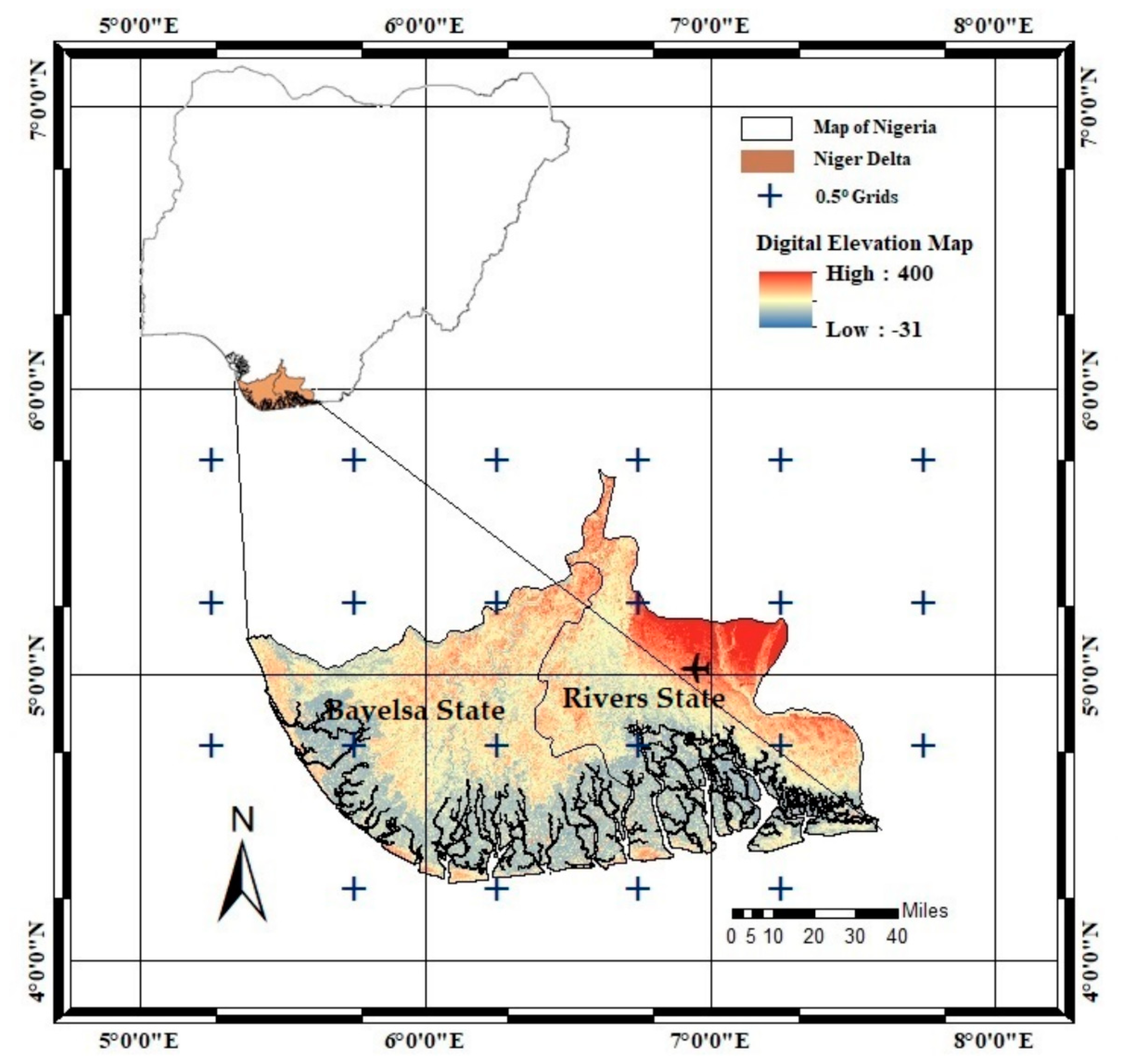
2.1. Description of the Study Area

The study area is located in the Niger Delta part of Nigeria and comprises Bayelsa and Rivers State (Figure 1). The area is a low lying coastal area drained by the Kwa-Ibo, Imo, Bonny, and Aba Rivers and their tributaries. The region has an equatorial climate toward the southern coast and subequatorial climate toward the northern tropical rainforest [36]. The elevation of the area under the influence of high coastal tides results in flooding, especially during the rainy season [37]. The area is characterized by typical tropical wet (March to October) and dry seasons (November to February) with a mean annual rainfall increasing from 2000 mm around the northern fringe to about 4500 mm around the coastal margin [38]. A short spell of the dry season, often referred to as the ‘August break’, caused by the deflection of the moisture-laden current, is often experienced in August or September [39].

The mean monthly temperatures are higher up to 26.67 °C around March/April and as low as 24.44 °C during July/August giving a small annual range of 2.73 °C. The mean relative humidity of the area is relatively high often reaching 90%, while the warm, wet southwesterly winds blow inland most of the year and the dust-laden, warm-dry northeasterly winds occasionally reach the coast for small periods of the year [40]. Recent studies have shown that during the last 20 years [41], a trend of an increase in prcp, Tmin and Tmax, and flood frequencies observed over the years in the Niger Delta due to global warming depicts a clear sign of climate change with a variable future climate over the region [42,43,44,45].

2.2. Data and Sources

2.2.1. Gridded Dataset

This study used the climate research unit (CRU) daily prcp, Tmax and Tmin datasets between the historic years of 1980 to 2005 over the Niger Delta part of Nigeria due to the scarcity of reliable long records of hydroclimatological station observations in the area. The CRU datasets are observation-based gridded prcp, Tmin and Tmax datasets, which are widely used because of their extensive spatial and temporal coverage extracted from the CRU version 4.01 global climate dataset [46,47,48]. They were found to be the best-fit datasets that replicated the distribution patterns, spatial, and temporal variability of the Niger Delta’s observed datasets [49]. The gridded datasets were re-gridded to a common spatial resolution of 0.5° × 0.5° following the agreed resolution of the GCMs. The daily CRU datasets were downloaded from (http://www.cru.uea.ac.uk) resulting in an equal number of grids (22 grids), which were spatially distributed across the study area. The observed station data had only one observation within the study area, with two other contributing stations outside the study area. The historic daily climate data (prcp, Tmin and Tmax) within the same grid locations that housed the observed meteorological station were downscaled to the station resolution. These datasets covered a time period of 1980–2005 for the historical period as the observed climate data; the GCM-simulated dataset covered the periods of 1950–2005 for the historical periods, and 2006–2099 for the future periods.

2.2.2. Coupled Model Inter-comparison Project Phase 5 (CMIP5) GCM Datasets

Twenty-six GCMs of ISI-MIP (Inter-Sectorial Impact Model Inter-Comparison Project) [50] models (

Table 1. General circulation models (GCMs) used in the study at 0.5° grid.

GCM No	GCM Name	Institute	Resolution
1	ACCESS1.3	Commonwealth Scientific and Industrial Research Organization–Bureau of Meteorology, Australia	1.9 × 1.2
2	CanCM4	Canadian Center for Climate Modelling and Analysis, Canada	2.8 × 2.8
3	CanESM2
4	CCSM4	National Centre for Atmospheric Research, USA	0.94 × 1.25
5	CMCC.CESM	Centro Euro-Mediterraneo sui Cambiamenti Climatici, Italy	0.7 × 0.7
6	CMCC.CMS		1.9 × 1.9
7	CNRM.CM5	Centre National de Recherches Météorologiques, Centre, France	1.4 × 1.4
8	CSIRO.Mk3.6.0	Commonwealth Scientific and Industrial Research Organization, Australia	1.9 × 1.9
9	CSIRO.Mk3L.1.2
10	GFDL.CM3	Geophysical Fluid Dynamics Laboratory, USA	2.5 × 2.0
11	GFDL.ESM2M
12	GISS.E2.H	NASA/GISS (Goddard Institute for Space Studies), USA	2.5 × 2.0
13	HadCM3	Met Office Hadley Centre, UK	1.9 × 1.2
14	HadGEM2.AO
15	HadGEM2.CC
16	HadGEM2.ES
17	INMCM4	Institute of Numerical Mathematics, Russia	2.0 × 1.5
18	IPSL.CM45A.LR	Institut Pierre Simon Laplace, France	2.5 × 1.3
19	IPSL.CM5A.MR		3.7 × 1.9
20	MIROC.ESM	The University of Tokyo, National Institute for Environmental Studies, and Japan Agency for Marine-Earth Science and Technology, Japan	2.8 × 2.8
21	MIROC.ESM.CHM
22	MIROC5		1.4 × 1.4
23	MPI.ESM.LR	Max Planck Institute for Meteorology, Germany	1.9 × 1.9
24	MPI.ESM.MR
25	MRI.CGCM3	Meteorological Research Institute, Japan	1.1 × 1.1
26	Noer.ESM1.M	Meteorological Institute, Norway	2.5 × 1.9

) and two carbon and other greenhouse, aerosols, etc., emission scenarios (RCP4.5 and RCP8.5) for the years (1980–2099) were downscaled for the basin in order to be consistent with the CRU dataset observations. The GCM data were obtained from the CMIP5 data portal website (http://pcmdi9.llnl.gov/). The GCMs were selected based on the availability of daily simulation for two representative concentration pathways (RCP), which were the RCP4.5 and RCP8.5 scenarios.

RCP4.5 is an intermediate pathway scenario that shows a good agreement with the latest policy of lower greenhouse gas emissions by the global community, while RCP8.5 is the business-as-usual scenario, which is consistent with a future that has no change in climate policy to reduce emissions [51]. Therefore, RCP4.5 and RCP8.5 were selected as these two scenarios can provide a possible complete range of impact. As the GCMs are available in different resolutions, all CMIP5 data were extracted and downscaled uniformly to the same spatial scale (0.5° × 0.5°) to reduce biases introduced by different resolutions for a fair comparison. This technique uses nearby areas to generate point output from each GCM at each grid point, thus providing a smooth interpolation that is widely used for the re-gridding of GCMs [48]. Table 1 gives an overview of the GCMs.

3. Methodology

The procedure for the identification and ranking of a subset of a GCM ensemble for simulation of the spatial and temporal projection of changes in rainfall and temperature for this study are outlined as follows:

• Extracting and re-gridding of the selected 26 GCM datasets and CRU gridded datasets to a spatial resolution of 0.5° × 0.5° was carried out.
• SU was then applied to evaluate and assess the association between the 26 GCMs and the CRU gridded observations (prcp, Tmax, and Tmin) at each of the 22 grid points of 0.5° × 0.5° resolution covering the study area (Figure 1), over the reference period 1980–2005.
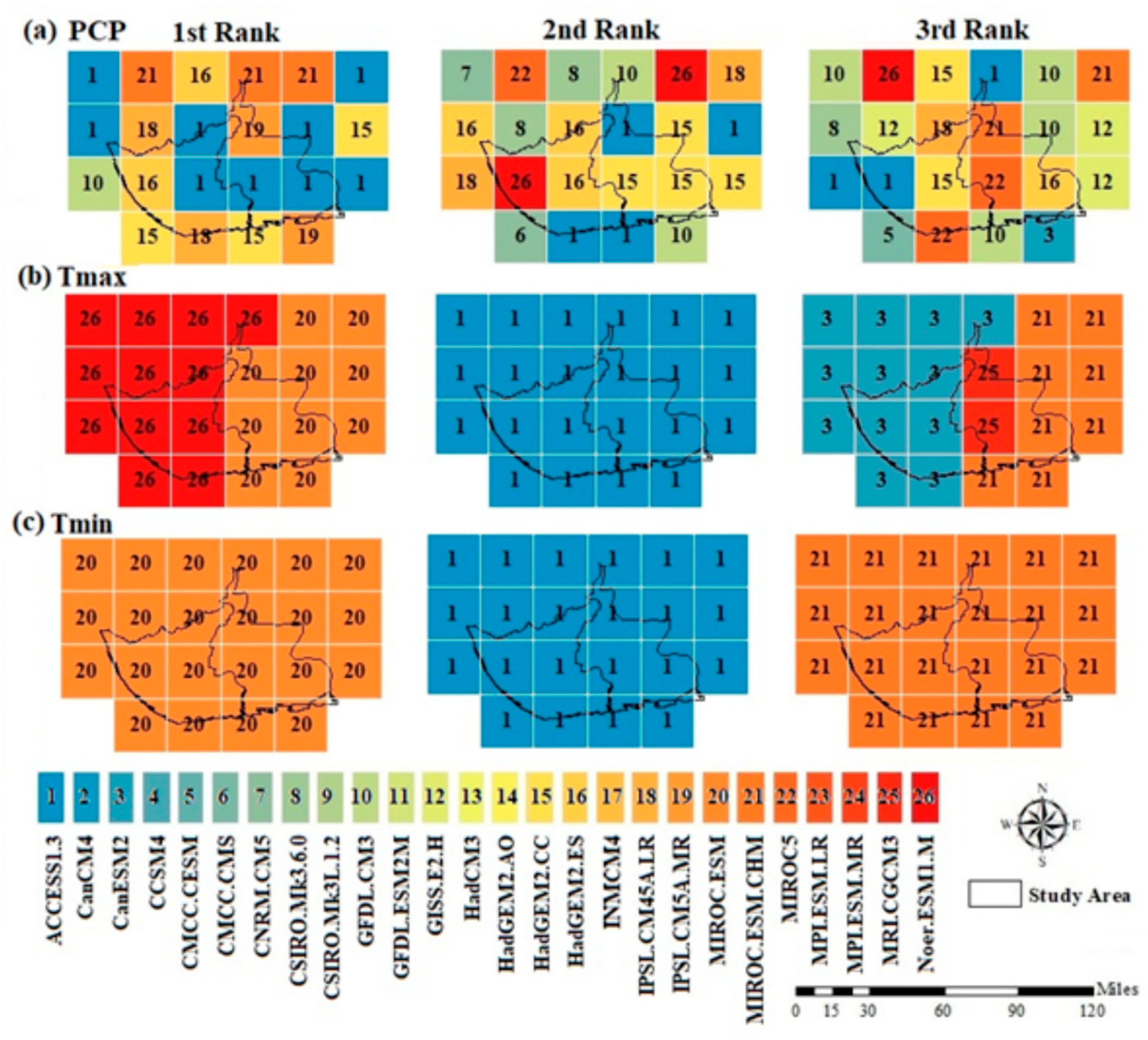
• The GCMs were then ranked based on the computed SU weight obtained at each grid points using the SU weighting technique, where a higher rank was given to GCMs with more weight in most of the grid points. A separate list of rank is prepared for each climatic variable (prcp, Tmax, and Tmin) and each gridded dataset (

  Table 2. Overall SU weights of GCMs and their ranks according to their ability to simulate the CRU prcp, Tmax, and Tmin datasets. The selected GCMs are shown in bold font.

  Ranks	GCMs	Prcp			Tmax			Tmin
  		SU	NSE	R2	SU	NSE	R2	SU	NSE	R2
  1	ACCESS1-3	0.28	0.58	0.81	0.15	0.67	0.84	0.09	0.86	0.55
  2	MIROC-ESM	0.14	0.63	0.84	0.10	0.87	0.44	0.12	0.62	0.49
  3	MIROC-ESM-CHM	0.15	0.69	0.56	0.11	0.86	0.86	0.02	0.50	0.58
  4	Noer-ESM1-M	0.13	0.57	0.82	0.14	0.82	0.89	0.05	0.38	0.48
  5	MIROC5	0.08	0.62	0.82	0.15	5.36	0.88	0.06	1.88	0.45
  6	HadGEM2-ES	0.19	0.59	0.81	0.03	0.88	0.91	0.02	0.54	0.53
  7	CanCM4	0.07	0.49	0.74	0.08	0.91	0.91	0.01	0.65	0.48
  8	MRI-CGCM3	0.06	0.55	0.78	0.11	0.70	0.87	0.03	0.48	0.51
  9	MPI-ESM-MR	0.06	0.35	0.78	0.05	0.75	0.87	0.02	0.49	0.51
  10	CMCC-CMS	0.08	0.55	0.78	0.11	0.63	0.79	0.04	0.31	0.45
  11	CNRM-CM5	0.10	0.44	0.73	0.07	0.64	0.81	0.01	0.28	0.51
  12	CanESM2	0.10	0.52	0.77	0.12	2.18	0.67	0.01	6.48	0.25
  13	IPSL-CM45A-LR	0.15	0.63	0.85	0.03	0.81	0.91	0	0.42	0.57
  14	HadGEM2-CC	0.21	0.58	0.82	0	0.90	0.90	0	0.63	0.45
  15	HadCM3	0.09	0.58	0.80	0	0.91	0.91	0	0.67	0.51
  16	CMCC-CESM	0.08	0.61	0.81	0.00	0.89	0.89	0	0.65	0.48
  17	IPSL-CM5A-MR	0.11	0.47	0.74	0	0.84	0.85	0	0.64	0.46
  18	GFDL-ESM2M	0.11	0.49	0.74	0.04	0.79	0.85	0	0.40	0.55
  19	CSIRO-Mk3L-1-2	0.05	0.31	0.60	0	0.89	0.89	0	0.68	0.53
  20	HadGEM2-AO	0.03	0.62	0.83	0	0.84	0.81	0	0.49	0.29
  21	GISS-E2-H	0.14	0.32	0.62	0	0.74	0.76	0	0.56	0.37
  22	MPI-ESM-LR	0.06	0.55	0.80	0	0.00	0.87	0	0.63	0.56
  23	CSIRO-Mk3-6-0	0.13	0.44	0.71	0.02	0.15	0.83	0	0.06	0.57
  24	INMCM4	0.05	0.42	0.68	0	0.60	0.69	0	0.54	0.42
  25	CCSM4	0.09	0.51	0.76	0	0.70	0.66	0	0.44	0.46
  26	GFDL-CM3	0.21	0.35	0.42	0	0.62	0.15	0	0.37	0.20

  The bold from numbers 1 to 12 is differentiating the best performed GCMs among the ranks.

  ).
• The overall GCM ranks were then derived (Equation (4)) considering all their ranks and the weights obtained at all 22 grids over the entire study area.
• The final ranks of all three datasets were determined based on the frequency of occurrence of each GCM to combine the overall ranks in order to obtain a single rank for each GCM valid for the entire study.
• For simplicity, the easiest and the most common method of bias correction was carried out for correction of the biases in the best-selected future GCM ensemble against the CRU gridded observations. The additive correction method was used for temperature bias correction while the multiplicative correction method was used to correct the biases in prcp for GCM simulations under the two RCP scenarios for the period 2010–2099.
• The ensemble of the best four performing GCMs was then used for the prediction of spatial, temporal, and seasonal changes in rainfall for three future periods (2010–2039, 2040–2069, and 2070–2099) against the historical period (1980–2005).

3.1. Model Selection Using Symmetrical Uncertainty

Symmetrical uncertainty (SU) is an information entropy-based filtering approach that measures the changes in entropy based on the concept of information entropy in order to assess the similarity or mutual information between the GCM and observed datasets [33,35]. The information entropy estimates the amount of information common between the two variables. For example, if P(X) and P(Y) are the probability density functions and P(X, Y) is the joint probability density function of A and B, then the entropy H between X and Y is given in Equation (1) below [35,52]:

$$H\left(X,Y\right)= {{\displaystyle \sum }}^{\text{}}P\left(X,Y\right)\log \frac{P\left(X,Y\right)}{P\left(X)\times P(Y\right)}$$

(1)

The relation of entropy and mutual information can then be used to solve the problem in different ways as follows; if H(X) denotes the entropy of X, then:

$$H\left(X\right)= -{{\displaystyle \int }}^{\text{}}P\left(X\right)\log \left(P\left(X\right)\right)dx$$

(2)

The common information between the two variables is estimated by H as the difference between the sum of the entropies. The amount by which the entropy of X decreases reflects additional information about X provided by Y, and is called information gain (IG), which is given by Equation (3) [53]. Information gain (IG) measures how much one random variable tells about another.

$$IG\left(X,Y\right)=H\left(X\right)-H\left(X,Y\right)$$

(3)

The H estimated using Equation (1) indicates the amount of mutual information between the observations and GCMs. If the variables are independent of each other, the IG is 0, while a higher value of IG indicates that the GCMs have a higher similarity to the gridded observations.

The IG is biased toward the variable having higher values. These biases are compensated for by dividing the IG value with the sum of the entropies of the random variables, which is referred to as SU. Therefore, SU provides an unbiased estimation of the degree of similarity or dissimilarity of a GCM with the corresponding observations regardless of the shape of the underlying distributions. The SU uses the following steps for GCM selection:

$$SU\left(X,Y\right)= 2\frac{IG\left(X,Y\right)}{H\left(X\right)+H\left(Y\right) }$$

(4)

where H(X) and H(Y) denotes the conditional entropies of X and Y, while H (X,Y) represents the joint entropy of X and Y, respectively. SU values vary between 0 and 1, where 1 refers to a perfect agreement between the observations and GCMs, while a value of 0 refers to no agreement between the observations and GCMs [54].

3.2. Ranking of GCMs Using the Weighting Method

Ranking of GCMs at a single grid point is a relatively simple task. However, assessment and classification of GCMs from multiple grid points become difficult as the exercise may display different degrees of accuracies at different grid points. This becomes more difficult when the underlying preference model, like weights assignable to different attributes for some parameters, are considered. To overcome these challenges, a technique that aggregates and combines information from different sources such as the weighting method [55], frequency of occurrence majority rule [56], and numerical averaging [13] can be employed. In this study, the ranks of the GCMs relating to each grid point were computed for each climate variable based on the computed SU weights for the 22 grid points, considering all 26 GCMs. These are then ranked based on the frequency of occurrence at different ranks [17].

Then, the overall weight (W_o) for each variable (i.e., P, Tmax, and Tmin) and each GCM was determined by multiplying the frequency of occurrence of each GCM at a particular rank with the computed SU weight corresponding to its rank and summing all the values obtained [12], as shown in Equation (5) below:

$$W_o=X_1\left(w_1\right)+X_2\left(w_2\right)+X_3\left(w_3\right)\dots \dots \dots +X_{28}\left(w_{28}\right)$$

(5)

where X represents the frequency of occurrence (e.g., X₁ corresponds to the frequency of occurrence of GCM at rank 1); w represents the weight corresponding to each rank; and Wo denotes the overall weight of each GCM.

The ensemble of the four top-ranked GCMs was then considered for the simulation of daily prcp, Tmax, and Tmin.

3.3. Bias Correction

Projected raw GCM typically contains biases when compared with observations [57]. Bias correction was carried out to correct the projected raw GCM output using the differences in the mean and variability between GCM and observed datasets. In this study, the biases in the daily time series of the variables (i.e., prcp, Tmin, and Tmax) from the four top-ranked GCM output were corrected using the easiest and the most common methods, which were the additive method for temperature and multiplicative method for prcp [48,58,59]. For temperature, the additive correction factor for each month was used, and the adjusted formula for modified daily temperature (Tmax and Tmin) is expressed in Equation (6).

$$T_{correcte{d}_{ij}}=T_{GC{M}_{ij}}+\left({\overline{T}}_{referenc{e}_{jk}}-{\overline{T}}_{GC{M}_{jk}}\right)$$

(6)

where T is the temperature; $\overline{T}$ is the long-term average temperature; and i, j, k are the day, month, and year counters, respectively. For prcp, a multiplicative correction factor for each month is used, and the modified daily rainfall is expressed in Equation (7):

$$P_{correcte{d}_{ij}}=P_{GC{M}_{ij}}\times \frac{{\overline{P}}_{referenc{e}_{jk}}}{{\overline{P}}_{GC{M}_{jk}}}$$

(7)

where P is the precipitation (mm day⁻¹), and $\overline{P}$ is the long-term average precipitation.

3.4. Performance Assessment

Performance of the ensemble from all 26 GCMs and 4 SU selected GCMs of prcp, Tmax, and Tmin were examined using the correlation coefficient (R²) (Equation (8)), Nash–Sutcliff efficiency (NSE) (Equation (9)), and root mean square error (RMSE) (Equation (10)), [60]. The correlation coefficient (R²) is a measure of how the ensemble GCMs are likely to be predicted by the model and is equivalent to the sample cross-correlation between ensemble GCMs and observed datasets, where the overbar denotes mean values.

$$R^2=\left[\frac{{{\displaystyle \sum }}_{i=1}^n\left(y_i-\overline{y}\right)\left(o_i-\overline{o}\right)}{\sqrt{\left[\left({{\displaystyle \sum }}_{i=1}^n{\left(y_i-\overline{y}\right)}^2\right)\left({{\displaystyle \sum }}_{i=1}^n{\left(o_i-\overline{o}\right)}^2\right)\right]}}\right]$$

(8)

where y and o are the predicted and observed values, respectively; and Nv is the number of target data used for testing.

The Nash–Sutcliff efficiency (NSE) indicates the goodness-of-fit of the simulated ensemble GCMs and observed data in line 1:1 and can range from −∞ to 1. NSE measures the predictive skill of a model relative to the mean of observations [60]. In this evaluation, the classification suggested by [61] is described as: NSE > 0.75 (model is appropriate and good); 0.36 < NSE < 0.75 (model is satisfactory); and NSE < 0.36 (model is unsatisfactory) was adopted.

$$NSE=1- \left[\frac{{{\displaystyle \sum }}_{i=1}^{n }{\left(Y_i^{obs}- Y_i^{sim}\right)}^2 }{{{\displaystyle \sum }}_{i=1}^n{(Y_i^{obs}-Y^{mean})}^2}\right]$$

(9)

where Y^iobs is the ith observation for the constituent being evaluated; Y^isim is the ith simulated value for the constituent being evaluated; Y^mean is the mean of observed data for the constituent being evaluated; and n is the total number of observations.

The root mean square error (RMSE) measures the global fitness of a predictive model.

$$RMSE= \sqrt{\frac{1}{n}{\displaystyle \sum }_{i=1}^n{\left(y_o-y_i\right)}^2}$$

(10)

where y and o are the observed and predicted values, respectively; and N_v is the number of target data used for testing.

4. Results and Discussion

4.1. Ranking of the GCMs

Time series GCM and CRU datasets for the period 1980–2005 were used to calculate the SU weights. The GCMs were then ranked according to the weight derived from the SU technique. The SU weights define the advantage of one GCM over the others in simulating the observations. The higher the coefficients, the better performance of the GCM of interest.

The overall scores attained by the GCMs over the entire study area was estimated using Equation (4), and the estimated scores for each GCM are shown in Table 2. In many cases, small SU weights were observed among the GCMs, mainly in prcp with zero weights, and in some cases observed in both Tmax and Tmin, which have also been reported in previous studies [17,62]. The smaller difference in SU values among the GCMs indicated that all GCMs performed well with a similar degree of accuracy in replicating observations.

4.2. Spatial Distribution of Top-Ranked GCMs

The SU filter was applied individually to the 26 GCM grid points (0.5° × 0.5°) for prcp, Tmax, and Tmin with CRU data over the study area. The spatial distribution of the GCM ensemble from the SU filter, which ranked as best, second-best, and third-best are shown in Figure 2a–c. The results obtained shows that ACCESS1.3 was found to be the best GCM in simulating prcp in the first rank, while no single GCM was found to dominate the study areas with prcp in the second and third rank. The spatial distribution of the SU GCMs shows that CSIRO.Mk3L.1.2 was found to dominate the first rank, IPSL.CM45A.LR was found to dominate the second rank, while GFDL.ESM2M was found to dominate the third rank in simulating both Tmax and Tmin GCMs over the entire study area. However, the distribution of SU GCMs shows that MIROC-ESM simulated both Tmax and Tmin in most of the study area.

Noer.ESM1-M was found to be the best in the western part of the area, while MIROC-ESM was found to be the best in the eastern part of the study area for the Tmax. ACCESS1.3 was also found to dominate the second rank for both Tmax and Tmin. No single GCM was found to dominate the study areas with prcp in the third rank. MIROC-ESM-CHM dominated the Tmin, while the CanESM2 was found to perform best in the western part of the area and MIROC.ESM.CHM was found to be the best in the southeastern part of the area for Tmax in the third rank.

4.3. Selection of GCM Ensemble

GCMs that can simulate both prcp, Tmax, and Tmin are considered more appropriate for climate change impact analysis [6,8]. Twelve GCM outputs (shown in bold) ranking from the best performing to the worst are summarized in Table 2; the SU filter shows that the top four performing GCMs were ACCESS1.3, MIROC-ESM, MIROC-ESM-CHM, and NorESM1-M. These results further verified [16], who suggested that GCMs should meet these criteria. The top four GCMs were selected according to their higher SU weight and common performance. Table 2 shows the overall GCMs ranks as well as their performances after bias correction in simulating the CRU prcp, Tmax, and Tmin obtained from the overall weights derived from SU coefficients. The overall scores can be treated independently as separate data points as each model is a myriad of discrete process representations.

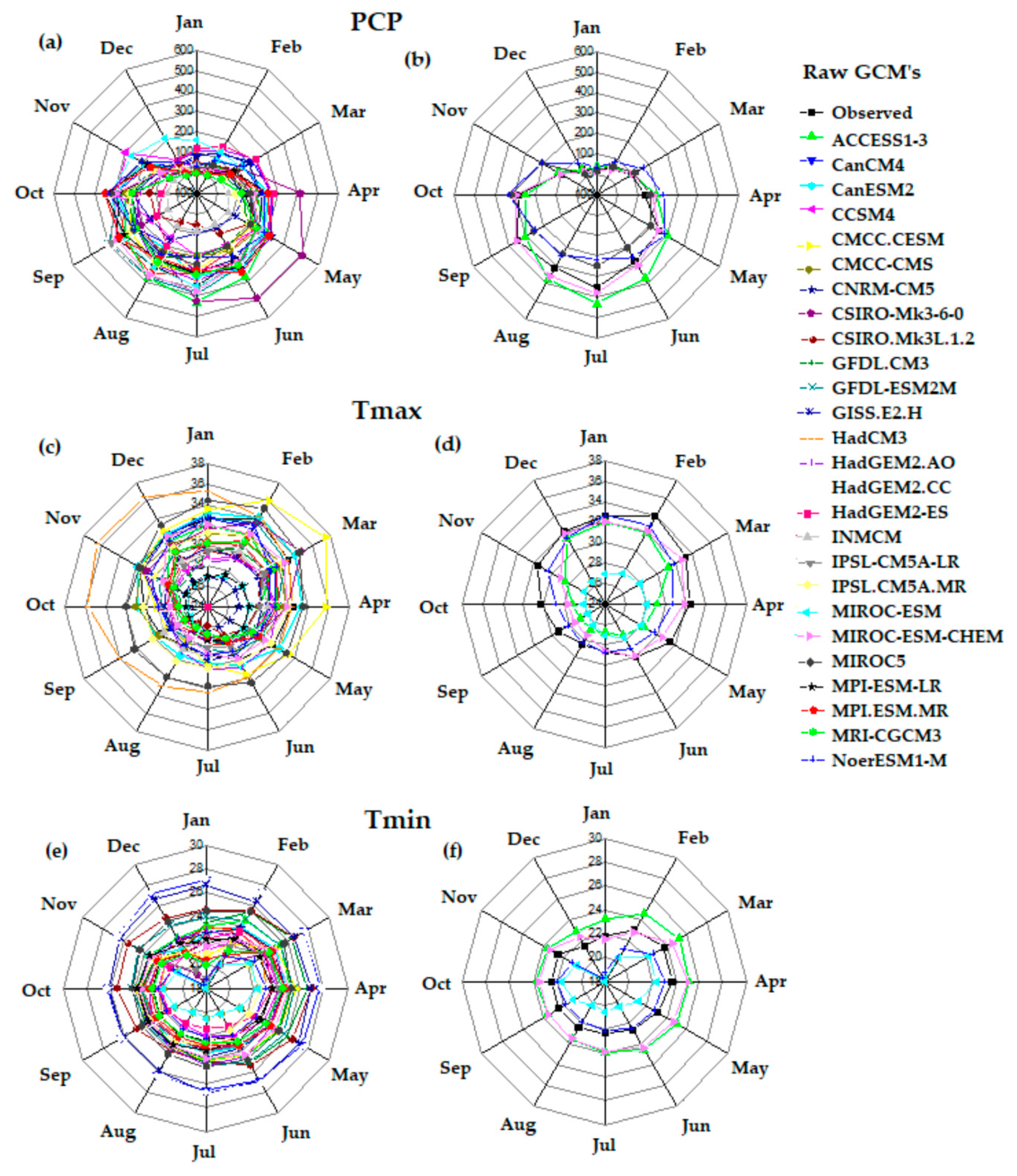
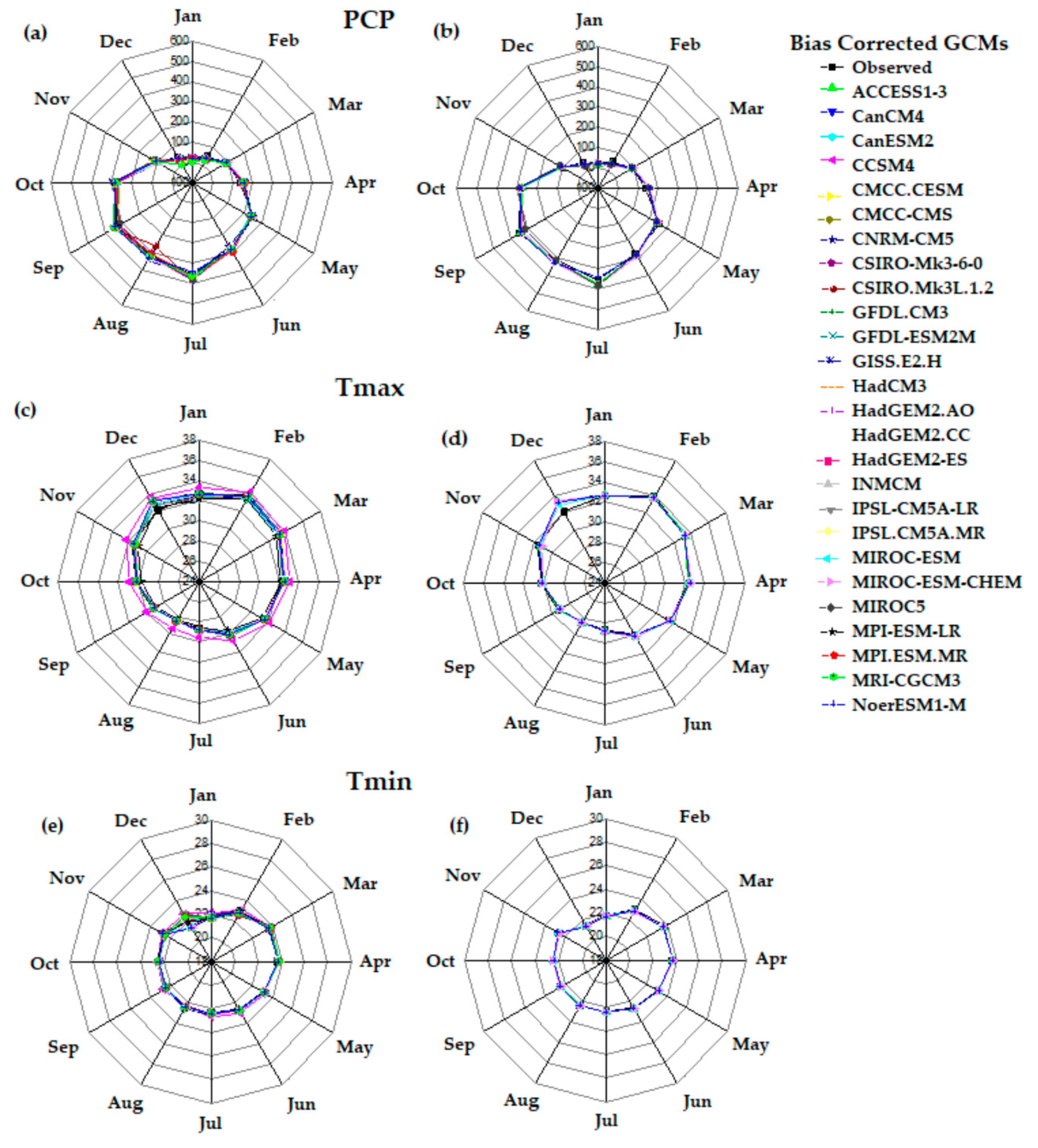
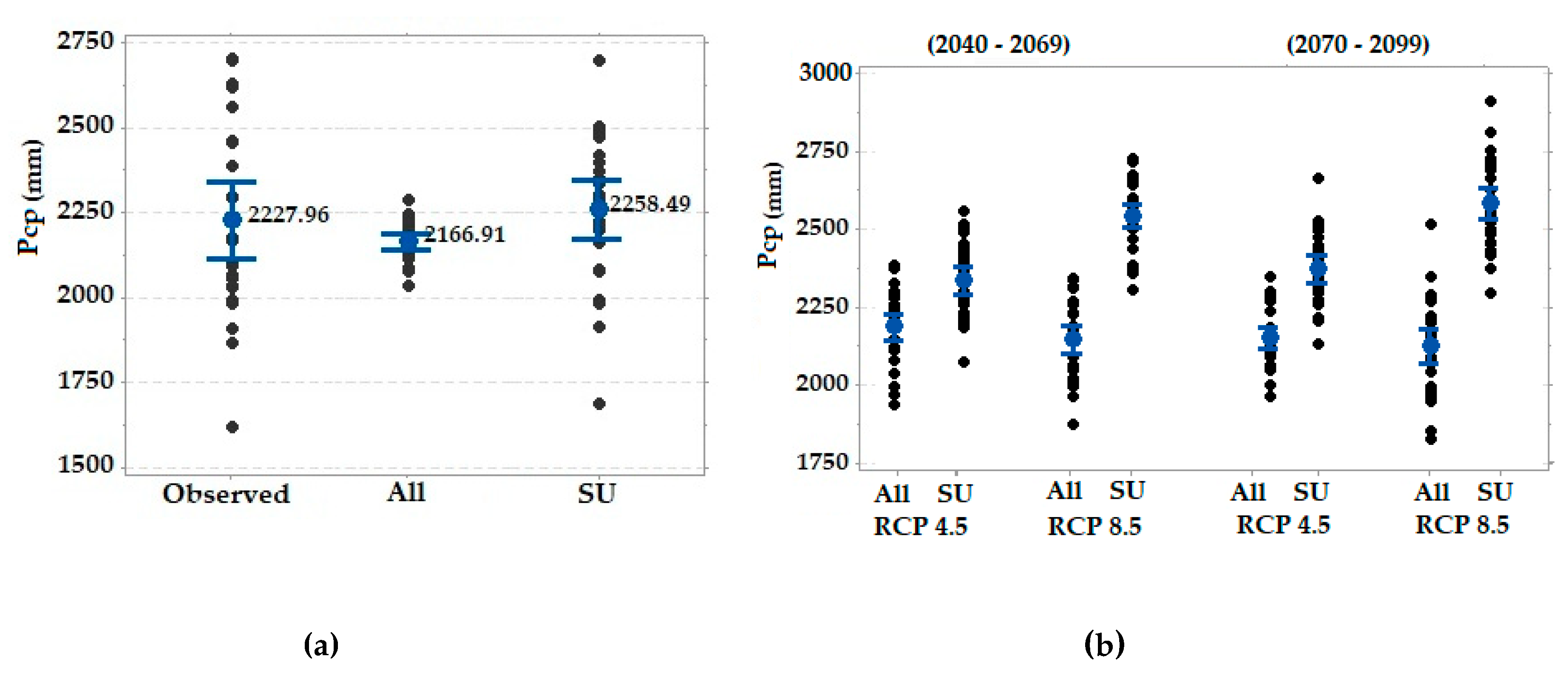
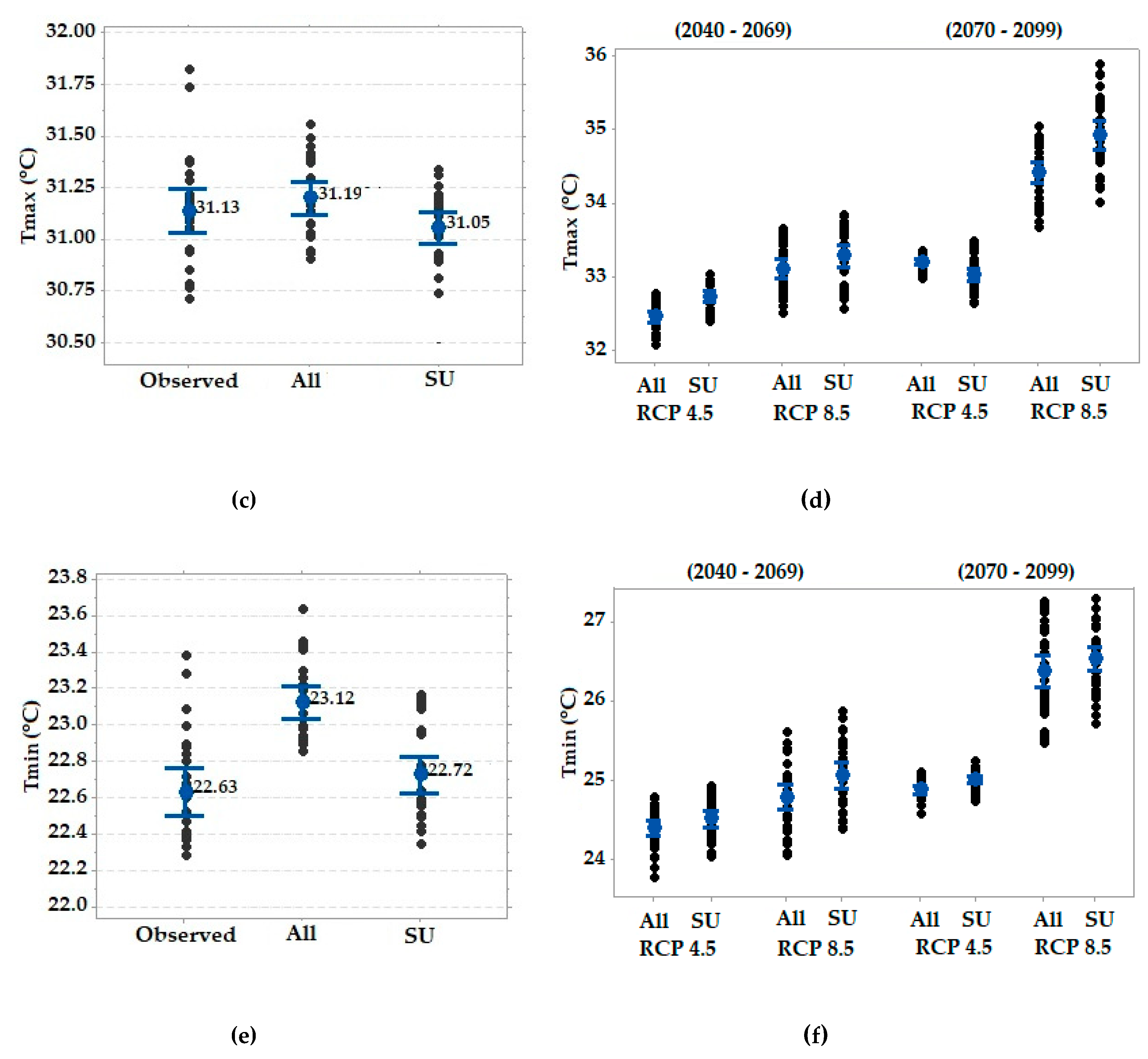
4.4. Ensemble Model Validation

The performance of the ensemble model at each grid point, for all 26 GCMs, four SU selected GCMs and CRU datasets were assessed by the coefficient of correlation (R²) and Nash–Sutcliff efficiency (NSE). As an example, the results obtained from the grid point in Port Harcourt is presented in

Table 3. Performance assessment of the GCM ensemble at the grid located in Port Harcourt.

Mean Annual	Observed		GCM Ensemble
			All	SU
Prcp (mm)	Sum	2227.95	2166.91	2255.49
	Mean	6.19	5.94	6.23
	RMSE	-	2.42	2.62
	NSE	-	0.58	0.62
	R2	-	0.86	0.83
Tmax (°C)	Mean	31.13	31.20	31.06
	RMSE	-	0.68	0.71
	NSE	-	1.00	1.00
	R2	-	0.92	0.92
Tmin (°C)	Mean	22.63	23.12	22.72
	RMSE	-	0.88	1.17
	NSE	-	1.00	1.00
	R2	-	0.64	0.62

. The results indicate that the ranking of GCMs assisted in identifying a better-performing GCM ensemble for the downscaling of simulations/projections and can be a possible way to produce more reliable hydroclimatic information at a finer spatial resolution and with reduced uncertainties.

Comparative plots of the mean monthly raw 26 GCMs and the four SU selected GCMs shown in Figure 3 show that the selected GCM outputs better matched the observed CRU datasets, which suggest a better performance after bias correction, as clearly proven in Figure 4. Results of the comparative analysis between the ensemble of all GCMs and the ensemble SU selected GCMs over the grid points as depicted in Table 3 showed a low RMSE with high NSE and R² values, which shows that the SU ensemble performed better in depicting the CRU datasets. The ensemble of all GCMs underestimated the sum (2166.91 mm) and the mean (5.94 mm) of CRU prcp (2227.95 mm and 6.19 mm), respectively. However, application of the SU filter in ensemble selection improved the results to a sum of 2255.49 mm and a mean of 6.23 mm. This trend was observed in all 22 grid points. A comparison of the mean values obtained at all the grid points for Tmax and Tmin confirmed the better performances of the SU model.

The seasonal averages of the bias-corrected 26 GCM output and the four selected models were compared to that of the CRU datasets in order to assess the performance of the downscaled model presented in Figure 4. The figures show that the selected GCMs better matched the CRU datasets after correcting the biases, which were assumed to indicate that they produced more realistic projections.

The obtained results were further validated using interval plots of changes in the annual averages of CRU datasets with the ensemble of all 26 GCMs and the four selected SU GCMs for prcp, Tmax, and Tmin (Figure 5). The changes and the levels of uncertainty were estimated using the RMSE and the 95% confidence band shows the spread of the uncertainties during the future periods. The results obtained indicated the efficiency of the SU ensemble models in GCM selection. Overall, the SU filter was found to perform well in improving GCM ensemble selection for simulating the sum and mean values in the region, as shown in Table 3.

The results showed a reproduction of the CRU observed datasets by the SU ensemble mean for Prcp, Tmax, and Tmin. This indicates that the SU ensemble selection approach can improve the accuracy in the projection by reducing uncertainties associated with individual GCMs.

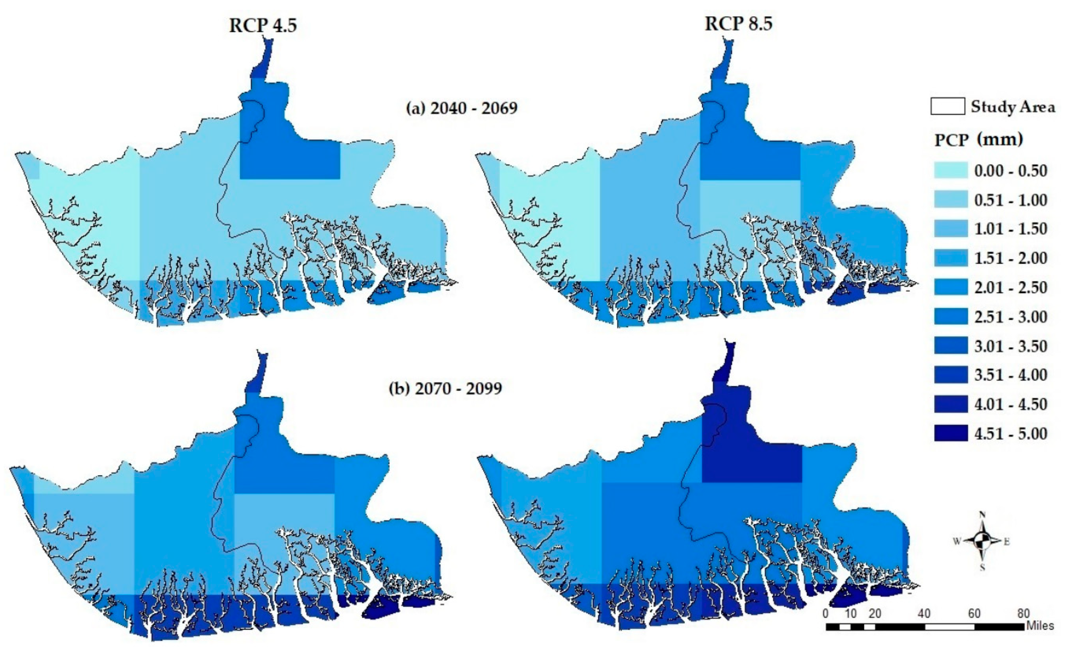
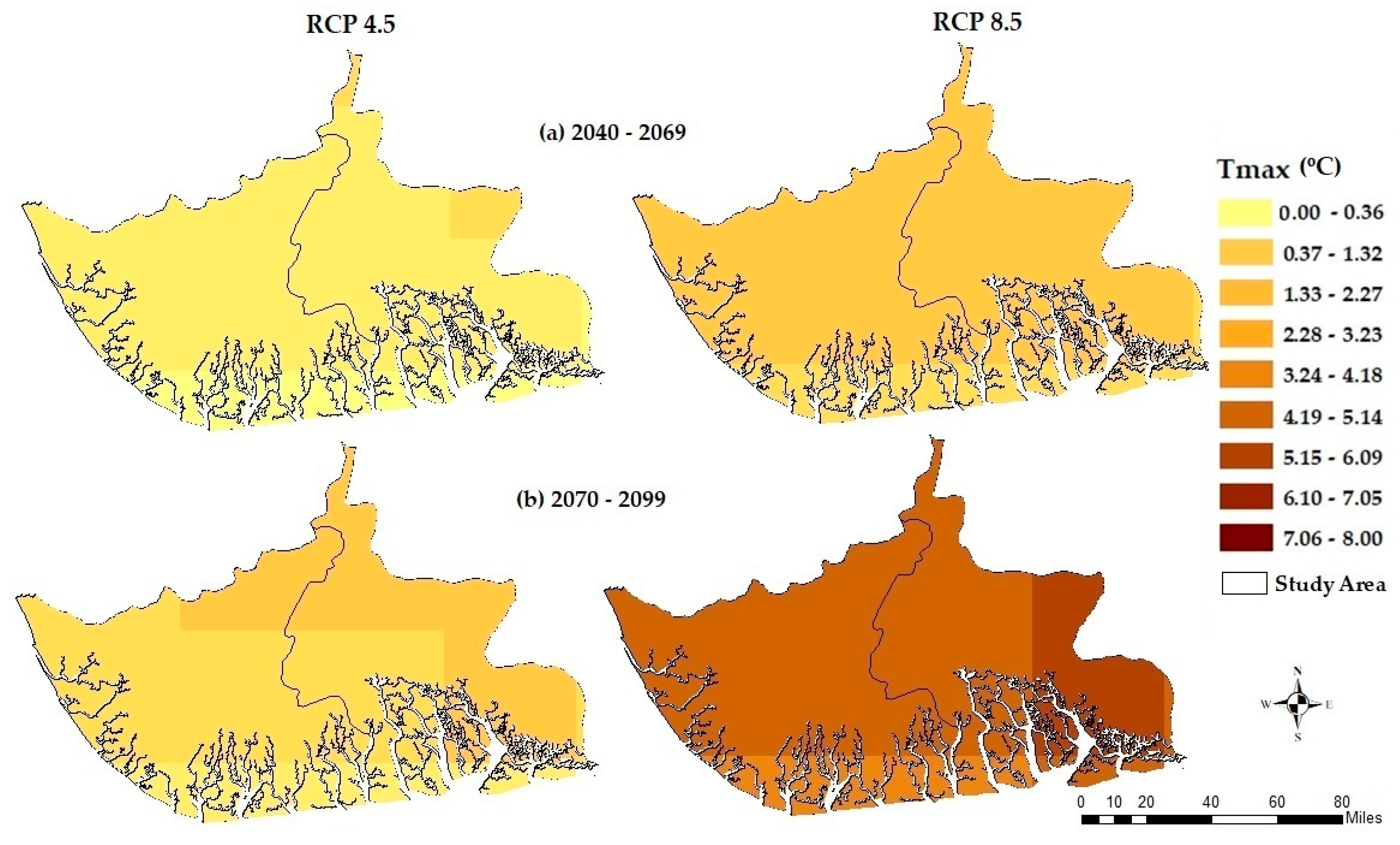
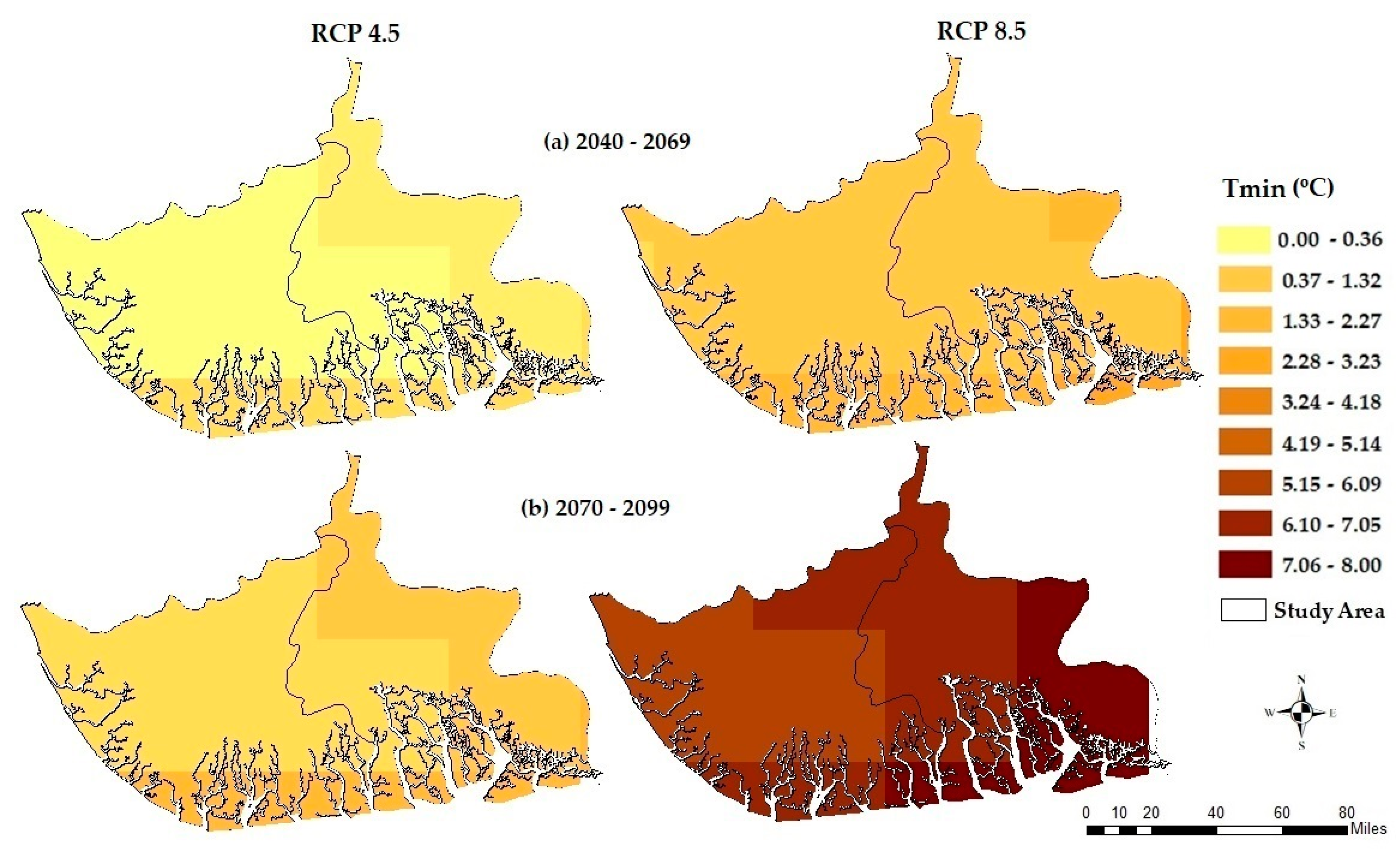
4.5. Spatial Changes in Mean Annual Prcp, Tmax, and Tmin

The SU selected GCM ensemble was used in this study to map the generated mean changes in Prcp, Tmax, and Tmin in the Niger Delta. To estimate these percentage changes, the averages of the CRU prcp, Tmax, and Tmin for the base period 1980–2005 at all grid points were subtracted from those of the projected prcp, Tmax, and Tmin for the different future periods, 2040–2069, and 2070–2099 as shown in Figure 6, Figure 7 and Figure 8 respectively.

Figure 6 shows the variation in prcp changes across the area. The coastal areas are generally projected to have the highest percentage of changes in prcp for all RCPs and future periods, while the northwestern part showed the lowest percentage changes. The changes in prcp ranged between 0.3% to 3.78% under RCP 4.5, and 1.62% to 4.74% under RCP8.5 for the period 2040–2069. During the period 2070–2099, a change between 0.26% to 3.57% under RCP4.5, and 0.7% to 4.94% under RCP8.5 was also projected across the study area.

The projected changes in annual Tmax and Tmin (Figure 7 and Figure 8) show an increasing trend across the study area for both future periods and RCPs. Tmax is projected to increase significantly by 3–8% (0.4 °C) under RCP4.5 and between 3.89-5.47% (1.25–1.79 °C) under RCP8.5 during the periods 2070–2099. Tmin is also expected to increase significantly by 0.31–2.52% (0.52 °C) under RCP4.5 and between 5.64–8.22% (1.38–2.02 °C) under RCP8.5 during the periods 2070–2099, as expected in response to greenhouse gases forcing, which is consistent with other parts of the world [63,64,65,66].

Based on the projected values of simulated climatic variables over the study area, the projected increase of this climate variable confirms the report of IPCC [1] as well as the studies by [36,67,68,69] in this region. These increase will further aggravate the vulnerability of the water quality, water resources, agricultural land, fisheries, and livestock in the Niger Delta coastal zone to climate change. The region might experience more extreme floods, which might threaten the livelihoods and socio-economic growth of the region, which might then also have a significant impact on Nigeria’s GDP as the primary source of the country’s revenue is the oil and gas from the study area.

5. Conclusions

A suitable set of GCM ensembles for simulating the spatio-temporal changes in both prcp, Tmin, and Tmax were selected based on their performances in simulating the observed CRU datasets using the symmetrical uncertainty (SU) filter using 26 GCM outputs under RCP4.5 and RCP8.5 emission scenarios. The study identified four GCMs, namely ACCESS1.3, MIROC-ESM, MIROC-ESM-CHM, and NorESM1-M as the most suitable set of GCMs for simulating both prcp, Tmax, and Tmin over the Niger Delta. Though several studies have been conducted to assess future changes in prcp, Tmax, and Tmin at global scales, only limited studies have been conducted in West Africa and Nigeria. This study, therefore, is the first attempt to employ a selection of suitable sets of daily GCMs to simulate both prcp, Tmin, and Tmax together for the spatiotemporal projection changes in the Niger Delta.

The findings of this study predicted an increase in both Tmin, Tmax, and prcp for both periods and RCPs. The predicted increase in future prcp and temperature is useful to inform all stakeholders of the need to regulate anthropogenic activities such as gas flaring, illegal refining of crude oil, and other petrochemical products, which release more CO₂ and other greenhouse gases into the atmosphere in this region. This study will be useful in sustainable environmental management in the extreme weather driven by emerging climate change in the coastal zones of the Niger Delta, Nigeria.

References

1. IPCC. Climate Change 2007: Impacts: Adaptation and Vulnerability: Contribution of Working Group II to the Fourth Assessment Report of the Intergovernmental Panel. 2007. Available online: https://doi.org/10.1256/004316502320517344 (accessed on 12 April 2019).
2. Northrop, P.J. A Simple, Coherent Framework for Partitioning Uncertainty in Climate Predictions. J. Clim. 2013, 26, 4375–4376. [Google Scholar] [CrossRef]
3. Ahmed, K.; Shahid, S.; Wang, X.; Nawaz, N.; Najeebullah, K. Evaluation of Gridded Precipitation Datasets over Arid Regions of Pakistan. Water 2019, 11. [Google Scholar] [CrossRef] [Green Version]
4. Sun, Q.; Miao, C.; Duan, Q.; Ashouri, H.; Sorooshian, S.; Hsu, K.L. A Review of Global Precipitation Data Sets: Data Sources, Estimation, and Intercomparisons. Rev. Geophys. 2018, 56, 79–107. [Google Scholar] [CrossRef] [Green Version]
5. Hijmans, R.J.; Cameron, S.E.; Parra, J.L.; Jones, P.G.; Jarvis, A. Very High Resolution Interpolated Climate Surfaces for Global Land Areas. Int. J. Climatol. 2005, 25, 1965–1978. [Google Scholar] [CrossRef]
6. Khan, N.; Shahid, S.; Ahmed, K.; Ismail, T.; Nawaz, N.; Son, M. Performance Assessment of General Circulation Model in Simulating Daily Precipitation and Temperature Using Multiple Gridded Datasets. Water 2018, 10. [Google Scholar] [CrossRef] [Green Version]
7. IPCC. Climate Change the IPCC Scientific Assessment. IPCC 1990, 414. [Google Scholar] [CrossRef] [Green Version]
8. Salman, S.A.; Shahid, S.; Ismail, T.; Ahmed, K.; Wang, X.J. Selection of Climate Models for Projection of Spatiotemporal Changes in Temperature of Iraq with Uncertainties. Atmos. Res. 2018, 213, 509–522. [Google Scholar] [CrossRef]
9. Chen, J.; Brissette, F.P.; Leconte, R. Uncertainty of Downscaling Method in Quantifying the Impact of Climate Change on Hydrology. J. Hydrol. 2011, 401, 190–202. [Google Scholar] [CrossRef]
10. Foley, A.M. Uncertainty in Regional Climate Modelling: A Review. Prog. Phys. Geogr. 2010, 34, 647–670. [Google Scholar] [CrossRef] [Green Version]
11. Lutz, A.F.; ter Maat, H.W.; Biemans, H.; Shrestha, A.B.; Wester, P.; Immerzeel, W.W. Selecting Representative Climate Models for Climate Change Impact Studies: An Advanced Envelope-Based Selection Approach. Int. J. Climatol. 2016, 36, 3988–4005. [Google Scholar] [CrossRef] [Green Version]
12. Ahmed, K.; Shahid, S.; Sachindra, D.A.; Nawaz, N.; Chung, E.S. Fidelity Assessment of General Circulation Model Simulated Precipitation and Temperature over Pakistan Using a Feature Selection Method. J. Hydrol. 2019, 573, 281–298. [Google Scholar] [CrossRef]
13. Lin, C.Y.; Tung, C.P. Procedure for Selecting GCM Datasets for Climate Risk Assessment. Terr. Atmos. Ocean. Sci. 2017, 28, 43–55. [Google Scholar] [CrossRef] [Green Version]
14. Knutti, R.; Masson, D.; Gettelman, A. Climate Model Genealogy: Generation CMIP5 and How We Got There. Geophys. Res. Lett. 2013, 40, 1194–1199. [Google Scholar] [CrossRef]
15. McSweeney, C.F.; Jones, R.G.; Lee, R.W.; Rowell, D.P. Selecting CMIP5 GCMs for Downscaling over Multiple Regions. Clim. Dyn. 2015, 44, 3237–3260. [Google Scholar] [CrossRef] [Green Version]
16. Abramowitz, G.; Herger, N.; Gutmann, E.; Hammerling, D.; Knutti, R.; Leduc, M.; Lorenz, R.; Pincus, R.; Schmidt, G.A. ESD Reviews: Model Dependence in Multi-Model Climate Ensembles: Weighting, Sub-Selection and out-of-Sample Testing. Earth Syst. Dyn. 2019, 10, 91–105. [Google Scholar] [CrossRef] [Green Version]
17. Srinivasa Raju, K.; Nagesh Kumar, D. Ranking General Circulation Models for India Using TOPSIS. J. Water Clim. Chang. 2015, 6, 288–299. [Google Scholar] [CrossRef] [Green Version]
18. Warszawski, L.; Frieler, K.; Huber, V.; Piontek, F.; Serdeczny, O.; Schewe, J. The Inter-Sectoral Impact Model Intercomparison Project (ISI–MIP): Project Framework. Proc. Natl. Acad. Sci. 2014, 111, 3228–3232. [Google Scholar] [CrossRef] [Green Version]
19. Shiru, M.S.; Shahid, S.; Chung, E.-S.; Alias, N.; Scherer, L. A MCDM-Based Framework for Selection of General Circulation Models and Projection of Spatio-Temporal Rainfall Changes: A Case Study of Nigeria. Atmos. Res. 2019, 225, 1–16. [Google Scholar] [CrossRef]
20. Chandrashekar, G.; Sahin, F. A Survey on Feature Selection Methods. Comput. Electr. Eng. 2014, 40, 16–28. [Google Scholar] [CrossRef]
21. Talavera, L. An Evaluation of Filter and Wrapper Methods for Feature Selection in Categorical Clustering. In International Symposium on Intelligent Data Analysis; Springer: Berlin, Germany, 2005; pp. 440–451. [Google Scholar]
22. Barfus, K.; Bernhofer, C. Assessment of GCM Capabilities to Simulate Tropospheric Stability on the Arabian Peninsula. Int. J. Climatol. 2015, 35, 1682–1696. [Google Scholar] [CrossRef]
23. Pierce, D.W.; Barnett, T.P.; Santer, B.D.; Gleckler, P.J. Selecting Global Climate Models for Regional Climate Change Studies. Proc. Natl. Acad. Sci. 2009, 106, 8441–8446. [Google Scholar] [CrossRef] [Green Version]
24. Ruan, Y.; Liu, Z.; Wang, R.; Yao, Z. Assessing the Performance of CMIP5 GCMs for Projection of Future Temperature Change over the Lower Mekong Basin. Atmosphere (Basel). 2019, 10, 93. [Google Scholar] [CrossRef] [Green Version]
25. Dudek, G. Tournament Searching Method to Feature Selection Problem. Lect. Notes Comput. Sci. (including Subser. Lect. Notes Artif. Intell. Lect. Notes Bioinformatics) 2010, 6114 LNAI, 437–444. [Google Scholar]
26. Hammami, D.; Lee, T.S.; Ouarda, T.B.M.J.; Le, J. Predictor Selection for Downscaling GCM Data with LASSO. J. Geophys. Res. Atmos. 2012, 117, 1–11. [Google Scholar] [CrossRef]
27. Sutha, K.; Tamilselvi, J. A Review of Feature Selection Algorithms for Data Mining Techniques. Int. J. Comput. Sci. Eng. 2015, 7, 63–67. [Google Scholar]
28. Perkins, S.E.; Pitman, A.J.; Holbrook, N.J.; McAneney, J. Evaluation of the AR4 Climate Models’ Simulated Daily Maximum Temperature, Minimum Temperature, and Precipitation over Australia Using Probability Density Functions. J. Clim. 2007, 20, 4356–4376. [Google Scholar] [CrossRef]
29. Jiang, X.; Waliser, D.E.; Xavier, P.K.; Petch, J.; Klingaman, N.P.; Woolnough, S.J.; Guan, B.; Bellon, G.; Crueger, T.; DeMott, C.; et al. Vertical Structure and Physical Processes of the Madden-Julian Oscillation: Exploring Key Model Physics in Climate Simulations. J. Geophys. Res. Atmos. 2015, 120, 4718–4748. [Google Scholar] [CrossRef]
30. Min, S.-K.; Hense, A. A Bayesian Assessment of Climate Change Using Multimodel Ensembles. Part II: Regional and Seasonal Mean Surface Temperatures. J. Clim. 2007, 20, 2769–2790. [Google Scholar] [CrossRef]
31. Shukla, J.; DelSole, T.; Fennessy, M.; Kinter, J.; Paolino, D. Climate Model Fidelity and Projections of Climate Change. Geophys. Res. Lett. 2006, 33, 3–6. [Google Scholar] [CrossRef] [Green Version]
32. Reichler, T.; Kim, J. How Well Do Coupled Models Simulate Today’s Climate? Bull. Am. Meteorol. Soc. 2008, 89, 303–311. [Google Scholar] [CrossRef]
33. Shannon, C.E. A Mathematical Theory of Communication. 2001, 5, 365–395. Available online: https://culturemath.ens.fr/sites/default/files/p3-shannon.pdf (accessed on 31 January 2020).
34. Ma, C.-W.; Ma, Y.-G. Shannon Information Entropy in Heavy-Ion Collisions. Prog. Part. Nucl. Phys. 2018, 99, 120–158. [Google Scholar] [CrossRef] [Green Version]
35. Singh, B.; Kushwaha, N.; Vyas, O.P. A Feature Subset Selection Technique for High Dimensional Data Using Symmetric Uncertainty. J. Data Anal. Inf. Process. 2014, 95–105. [Google Scholar] [CrossRef] [Green Version]
36. Matemilola, S.; Adedeji, O.H.; Elegbede, I.; Kies, F. Mainstreaming Climate Change into the EIA Process in Nigeria: Perspectives from Projects in the Niger Delta Region. Climate 2019, 7. [Google Scholar] [CrossRef] [Green Version]
37. Amadi, A.N. Impact of Gas-Flaring on the Quality of Rain Water, Groundwater and Surface Water in Parts of Eastern Niger Delta, Nigeria. J. Geosci. Geomatics 2014, 2, 114–119. [Google Scholar]
38. Adejuwon, J.O. Rainfall Seasonality in the Niger Delta Belt, Nigeria. J. Geogr. Reg. Plan. 2012, 5, 51–60. [Google Scholar]
39. Amadi, A.N.; Olasehinde, P.I.; Nwankwoala, H.O. Hydrogeochemistry and Statistical Analysis of Benin Formation in Eastern Niger Delta, Nigeria. Int. Res. J. Pure Appl. Chem. 2014, 4, 327–338. [Google Scholar] [CrossRef]
40. Ituen, E.U.; Alonge, A.F. Niger Delta Region of Nigeria, Climate Change and the Way Forward. In Proceedings of the Bioenergy Engineering, Bellevue, DC, USA, 11–14 October 2009. [Google Scholar]
41. Prince, C.; Mmom, P.C.M. Vulnerability and Resilience of Niger Delta Coastal Communities to Flooding. IOSR J. Humanit. Soc. Sci. 2013, 10, 27–33. [Google Scholar] [CrossRef]
42. Amangabara, G.; Obenade, M. Flood Vulnerability Assessment of Niger Delta States Relative to 2012 Flood Disaster in Nigeria. Am. J. Environ. Prot. 2015, 3, 76–83. [Google Scholar]
43. Ologunorisa, T.E.; Tersoo, T. The Changing Rainfall Pattern and Its Implication for Flood Frequency in Makurdi, Northern Nigeria. J. Appl. Sci. Environ. Manag. 2006, 10, 97–102. [Google Scholar] [CrossRef] [Green Version]
44. Ologunorisa, T.E.; Adeyemo, A. Public Perception of Flood Hazard in the Niger Delta, Nigeria. Environmentalist 2005, 25, 39–45. [Google Scholar] [CrossRef]
45. Tawari-fufeyin, P.; Paul, M.; Godleads, A.O. Some Aspects of a Historic Flooding in Nigeria and Its Effects on Some Niger-Delta Communities. Am. J. Water Resour. 2015, 3, 7–16. [Google Scholar]
46. Harris, I.; Jones, P.D.; Osborn, T.J.; Lister, D.H. Updated High-Resolution Grids of Monthly Climatic Observations - the CRU TS3.10 Dataset. Int. J. Climatol. 2014, 34, 623–642. [Google Scholar] [CrossRef] [Green Version]
47. Jones, P.D.; Harris, I.C. Climatic Research Unit (CRU) Time-Series Datasets of Variations in Climate with Variations in Other Phenomena. NCAS British Atmospheric Data Centre, 2008. Available online: http://catalogue.ceda.ac.uk/uuid/3f8944800cc48e1cbc29a5ee12d8542d (accessed on 13 June 2019).
48. Ashraf Vaghefi, S.; Abbaspour, N.; Kamali, B.; Abbaspour, K.C. A Toolkit for Climate Change Analysis and Pattern Recognition for Extreme Weather Conditions–Case Study: California-Baja California Peninsula. Environ. Model. Softw. 2017, 96, 181–198. [Google Scholar] [CrossRef]
49. Hassan, I.; Kalin, R.M.; White, C.J.; Aladejana, J.A. Evaluation of Daily Gridded Meteorological Datasets over the Niger Delta Region of Nigeria and Implication to Water Resources Management. Clim. Sci. SCRIP 2020. Available online: https://www.scirp.org/journal/paperinformation.aspx?paperid=97271 (accessed on 24 December 2019).
50. Hempel, S.; Frieler, K.; Warszawski, L.; Schewe, J.; Piontek, F. A Trend-Preserving Bias Correction—The ISI-MIP Approach. Earth Syst. Dyn. 2013, 4, 219–236. [Google Scholar] [CrossRef] [Green Version]
51. Wang, L.; Ranasinghe, R.; Maskey, S.; van Gelder, P.H.A.J.M.; Vrijling, J.K. Comparison of Empirical Statistical Methods for Downscaling Daily Climate Projections from CMIP5 GCMs: A Case Study of the Huai River Basin, China. Int. J. Climatol. 2016, 36, 145–164. [Google Scholar] [CrossRef]
52. Piao, M.; Piao, Y.; Lee, J.Y. Symmetrical Uncertainty-Based Feature Subset Generation and Ensemble Learning for Electricity Customer Classification. Symmetry (Basel). 2019, 11, 498. [Google Scholar] [CrossRef] [Green Version]
53. Adami, C. Information Theory in Molecular Biology. Phys. Life Rev. 2004, 1, 3–22. [Google Scholar] [CrossRef] [Green Version]
54. Shreem, S.S.; Abdullah, S.; Nazri, M.Z.A. Hybrid Feature Selection Algorithm Using Symmetrical Uncertainty and a Harmony Search Algorithm. Int. J. Syst. Sci. 2016, 47, 1312–1329. [Google Scholar] [CrossRef]
55. Roszkowska, E. Rank Ordering Criteria Weighting Methods-a Comparative Overview 2 5. Optimum. Stud. Ekon. 2013, 5, 65. [Google Scholar] [CrossRef]
56. Balinski, M.; Laraki, R. Majority Judgment vs. Majority Rule; Springer: Berlin Heidelberg, 2019; Available online: https://doi.org/10.1007/s00355-019-01200-x (accessed on 28 October 2019).
57. Mehrotra, R.; Sharma, A. Correcting for Systematic Biases in Multiple Raw GCM Variables across a Range of Timescales. J. Hydrol. 2015, 520, 214–223. [Google Scholar] [CrossRef]
58. Beyer, R.; Krapp, M.; Manica, A. A Systematic Comparison of Bias Correction Methods for Paleoclimate Simulations. Clim. Past Discuss. 2019, 1–23. [Google Scholar] [CrossRef]
59. Xu, Y. Hydrology and Climate Forecasting R Package for Data Analysis and Visualization. 2018. Available online: https://cran.r-project.org/web/packages/hyfo/vignettes/hyfo.pdf (accessed on 30 April 2019).
60. Moriasi, D.N.; Arnold, J.G.; Van Liew, M.W.; Bingner, R.L.; Harmel, R.D.; Veith, T.L. Model Evaluation Guidelines for Systematic Quantification of Accuracy in Watershed Simulations. Am. Soc. Agric. Biol. Eng. 2007, 50, 885–900. [Google Scholar]
61. Motovilov, Y.G.; Gottschalk, L.; Engeland, K.; Rodhe, A. Validation of a Distributed Hydrological Model against Spatial Observations. Agric. For. Meteorol. 1999, 99. [Google Scholar] [CrossRef]
62. Srinivasa Raju, K.; Sonali, P.; Nagesh Kumar, D. Ranking of CMIP5-Based Global Climate Models for India Using Compromise Programming. Theor. Appl. Climatol. 2017, 128, 563–574. [Google Scholar] [CrossRef]
63. Krinner, G.; Germany, F.; Shongwe, M.; Africa, S.; France, S.B.; Uk, B.B.B.B.; Germany, V.B.; Uk, O.B.; France, C.B.; Uk, R.C.; et al. Long-Term Climate Change: Projections, Commitments and Irreversibility. In Climate Change 2013-The Physical Science Basis: Contribution of Working Group I to the Fifth Assessment Report of the Intergovernmental Panel on Climate Change; Cambridge University Press: New York, NY, USA, 2013; pp. 1029–1136. [Google Scholar]
64. Expósito, F.J.; González, A.; Pérez, J.C.; Díaz, J.P.; Taima, D. High-Resolution Future Projections of Temperature and Precipitation in the Canary Islands. J. Clim. 2015, 28, 7846–7856. [Google Scholar] [CrossRef]
65. Rangwala, I.; Miller, J.R. Climate Change in Mountains: A Review of Elevation-Dependent Warming and Its Possible Causes. Clim. Change 2012, 114, 527–547. [Google Scholar] [CrossRef]
66. Martín, J.L.; Bethencourt, J.; Cuevas-Agulló, E. Assessment of Global Warming on the Island of Tenerife, Canary Islands (Spain). Trends in Minimum, Maximum and Mean Temperatures since 1944. Clim. Change 2012, 114, 343–355. [Google Scholar] [CrossRef]
67. Agumagu, O.; Todd, M. Modelling the Climatic Variability in the Niger Delta Region: Influence of Climate Change on Hydrology. Earth Sci. Clim. Chang. 2015, 6. [Google Scholar] [CrossRef] [Green Version]
68. Obroma Agumagu, O.A. Projected Changes in the Physical Climate of the Niger Delta Region of Nigeria. SciFed J. Glob. Warm. 2018. Available online: https://pdfs.semanticscholar.org/c5e7/17ebcd21acd09109553f3c11804f94ece611.pdf?_ga=2.9422967.312418545.1579023164-1793679239.1552909823 (accessed on 1 May 2019).
69. Ike, P.C.; Emaziye, P.O. An Assessment of the Trend and Projected Future Values of Climatic Variables in Niger Delta Region, Nigeria. 2012, 4, 165–170. Available online: https://www.researchgate.net/profile/Pius_Ike/publication/268202347_An_Assessment_of_the_Trend_and_Projected_Future_Values_of_Climatic_Variables_in_Niger_Delta_Region_Nigeria/links/5b008a9ba6fdccf9e4f56f9a/An-Assessment-of-the-Trend-and-Projected-Future-Values-of-Climatic-Variables-in-Niger-Delta-Region-Nigeria.pdf (accessed on 12 April 2019).
Figure 1. Map of the study area showing the spatial distribution of 0.5° × 0.5° grids.
Water 12 00385 g001
Figure 2. The spatial distribution of GCMs ranked best, second-best, and third-best position using a symmetrical uncertainty filter at different gird points for Prcp, Tmax, and Tmin over the Niger Delta.
Water 12 00385 g002
Figure 3. Monthly averages of CRU and raw datasets. (a) 26 Prcp, (b) 4 Prcp SU, (c) 26 Tmax, (d) 4 Tmax SU, (e) 26 Tmin, and (f) 4 Tmin SU GCM outputs for the historical period 1980–2005 at the grid point located in Port Harcourt.
Water 12 00385 g003
Figure 4. Monthly averages of CRU and bias corrected datasets. (a) 26 Prcp, (b) 4 Prcp SU, (c) 26 Tmax, (d) 4 Tmax SU, (e) 26 Tmin, and (f) 4 Tmin SU GCM outputs for the historical period 1980–2005 at the grid point located in Port Harcourt.
Water 12 00385 g004
Figure 5. Interval plots for the annual averages of CRU datasets with the ensemble of all 26 GCMs and the four SU selected GCMs for (a) Prcp (base period), (b) Prcp (future periods), (c) Tmax (base period), (d) Tmax (future periods), (e) Tmin (base period), and (f) Tmin (future periods) with 95% confidence interval at the grid located in Port Harcourt.
Water 12 00385 g005aWater 12 00385 g005b
Figure 6. Spatial distribution of percentage changes in average annual prcp, for periods (a) 2040–2069 and (b) 2070–2099 compared to the base period 1980–2005 for RCP4.5 and RCP8.5.
Water 12 00385 g006
Figure 7. Spatial distribution of percentage changes in average annual maximum temperature for periods (a) 2040–2069 and (b) 2070–2099 compared to the base period 1980–2005 for RCP4.5 and RCP8.5.
Water 12 00385 g007
Figure 8. Spatial distribution of percentage changes in average annual minimum temperature for periods (a) 2040–2069 and (b) 2070–2099 compared to the base period 1980–2005 for RCP4.5 and RCP8.5.
Water 12 00385 g008