Short-Term Multi-Objective Optimal Operation of Reservoirs to Maximize the Benefits of Hydropower and Navigation

Abstract
:1. Introduction
2. Navigation Capacity Evaluation
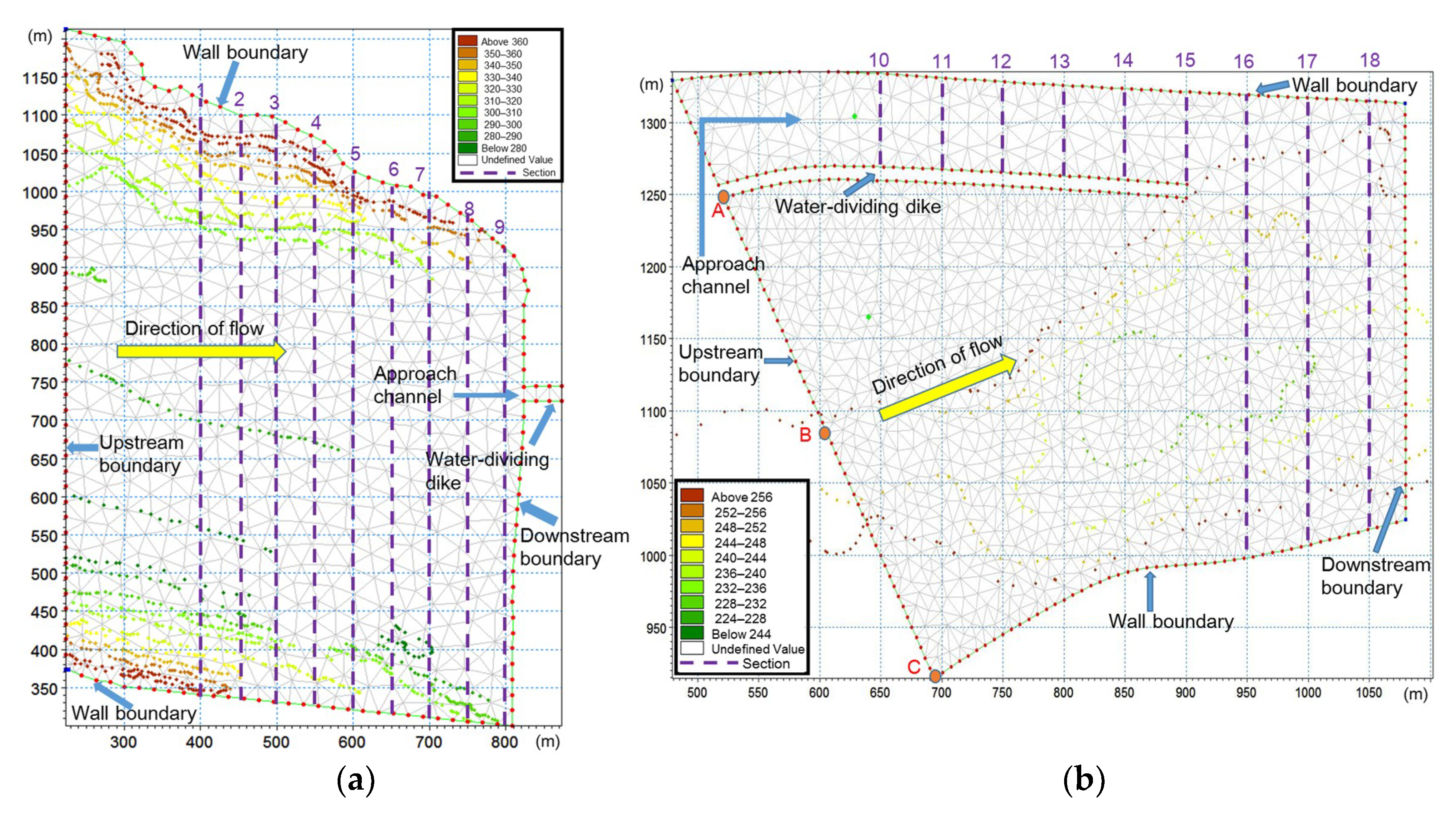
2.1. Hydrodynamic Model
2.2. Analysis of the Flow Velocity
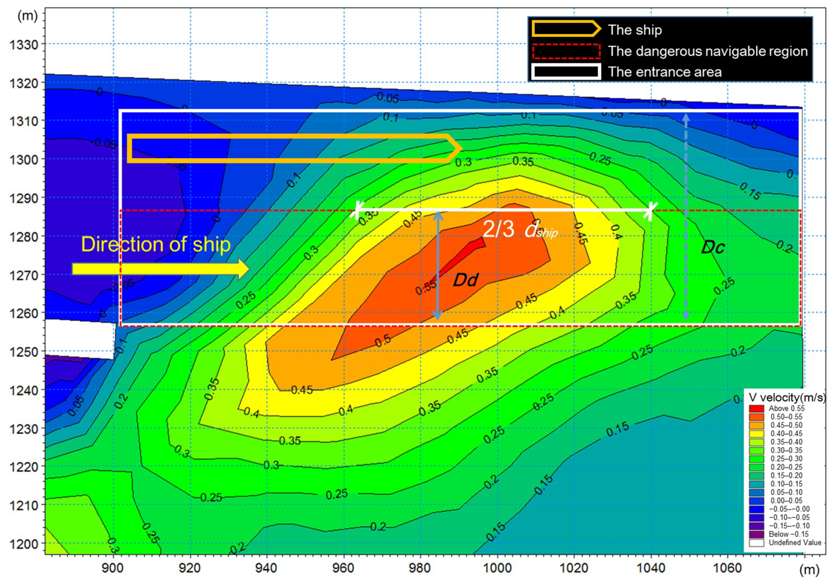
2.2.1. The Dangerous Navigation Area of Channel
2.2.2. The Navigation Capacity Considering the Flow Velocity ()
2.3. Analysis of the Variation of Water Level
3. Multi-Objective Reservoir Operation Model
3.1. Objective Function
3.1.1. Economic Objective: Maximizing the Daily Total Power Generation
3.1.2. Navigation Objective: Maximizing the Navigation Capacity
3.2. Constraints
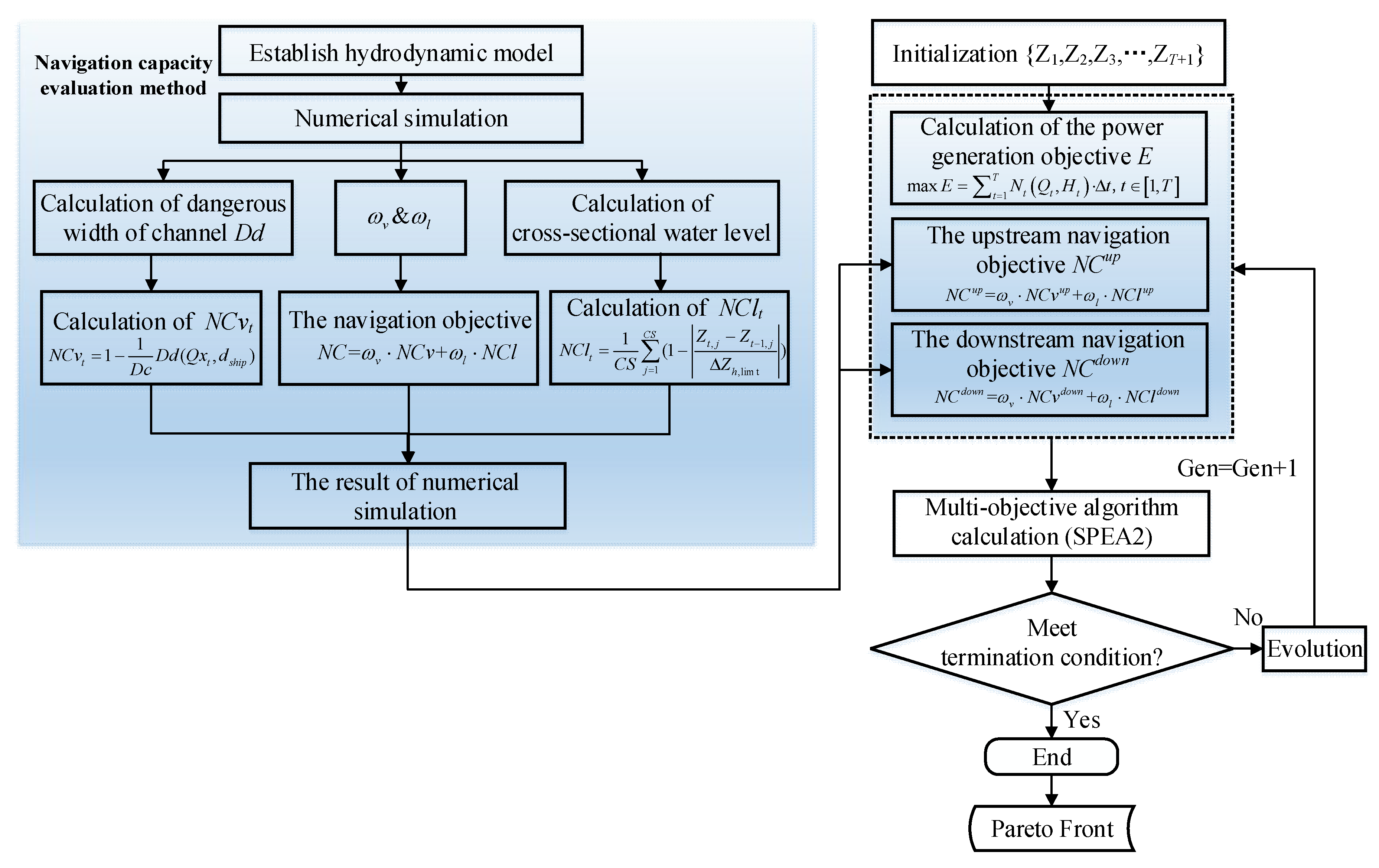
4. Methodology
- (1)
- When there are no individuals in the external archive set, the non-dominated solutions generated in the iteration are stored directly in the archive set;
- (2)
- If the newly generated individuals are dominated by the individuals in the archive set, the new individuals will be deleted. Conversely, individuals can be deleted from the original archive set and new individuals added to the archive set;
- (3)
- When the number of individuals in the archive set reaches the preset maximum capacity, the individuals with smaller crowding distance are deleted.
5. Case Study
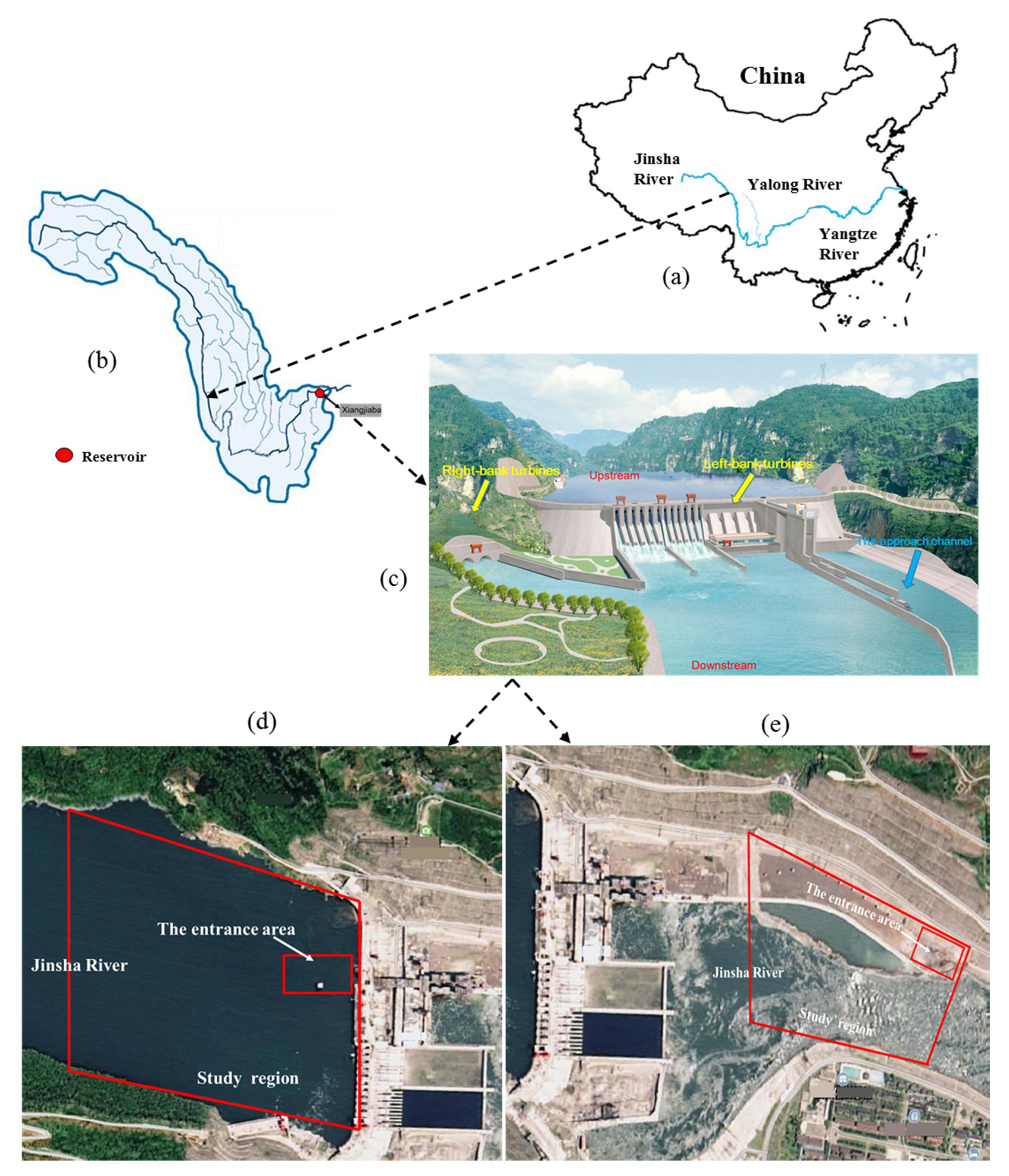
5.1. Case Description
5.2. Parameter Settings and Simulation Working Conditions
5.2.1. Model Parameter Setting
5.2.2. Simulation Working Conditions
5.3. Results
5.3.1. Numerical Simulation Results
- (1)
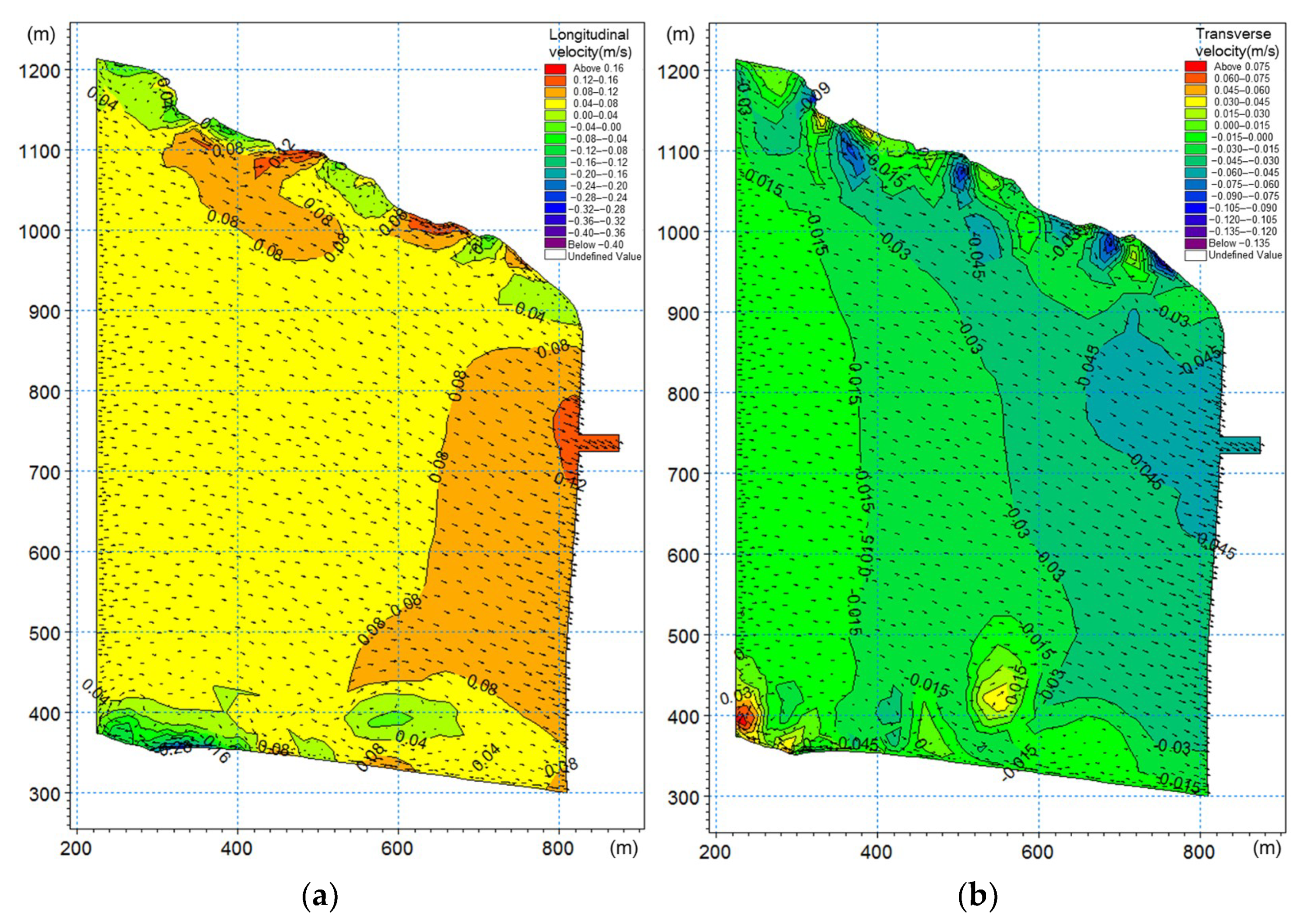
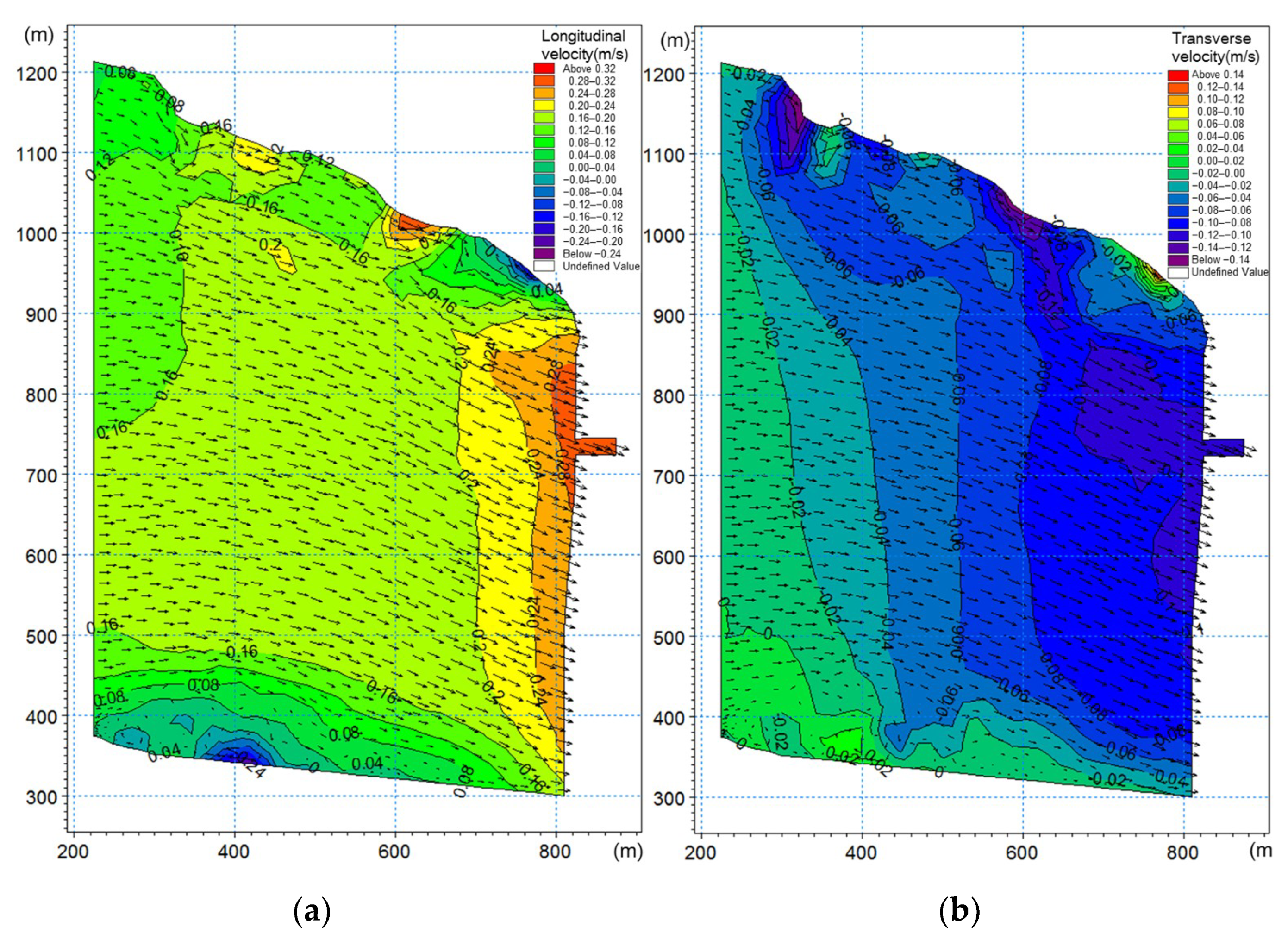
- The numerical simulation results of Condition P1 and Condition P2 are shown in Table 3, Figure 5, and Figure 6. It can be seen that the longitudinal velocity and transverse velocity of the upstream entrance area of approach channel satisfy the navigation requirements. Therefore, it can be inferred that the upstream navigation capacity () is less affected by the flow velocity. In this study case, is mainly related to the water level variation, and the formula for is expressed as follows:where: = 12 and = 1.5 m/h.
- (2)
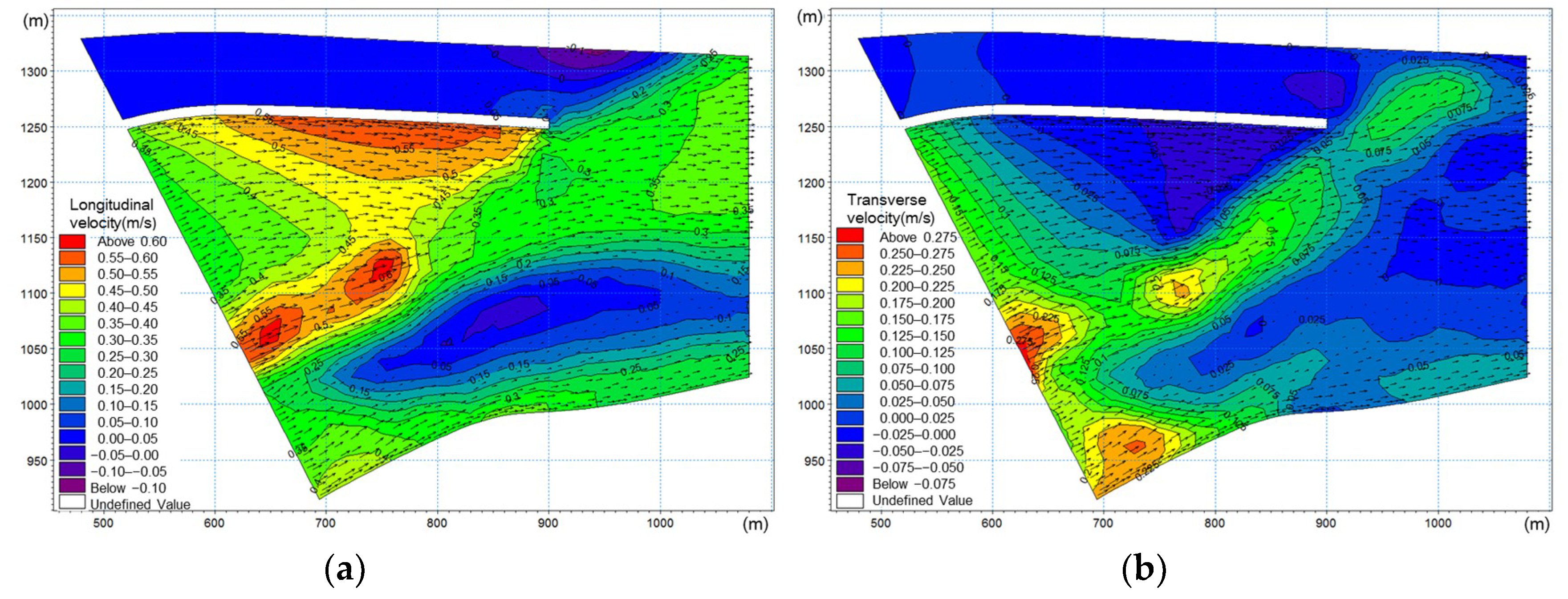
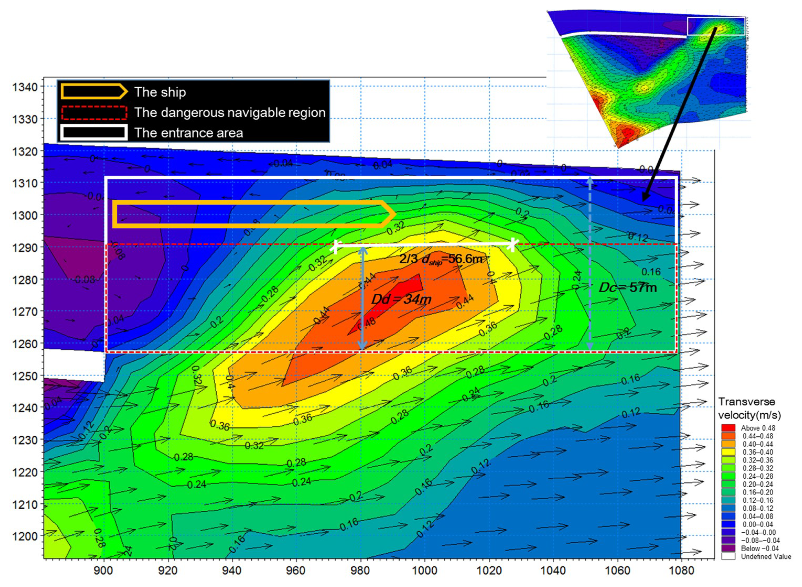
- The transverse velocity and longitudinal velocity in Condition P3 and the longitudinal velocity in the Condition P4 are all satisfied by the navigation requirement, as shown in Figure 7 and Table 3. However, the local transverse velocity exceeds the limit value of 0.3 m/s in the Condition P4, which seriously hinders the navigation in the entrance area of the approach channel. As a result, the transverse velocity is the most important factor affecting the downstream navigation, which is considered in this case.
- (1)
- For downstream navigation of XJB reservoir, when the discharge volume (less than 1700 m3/s) is relatively small, the downstream navigation capacity considering the flow velocity () of the three working conditions is the same ( = 1);
- (2)
- When the discharge volume is large (greater than 1700 m3/s), the is the poorest in Condition 1 (only left-bank turbines work), better in Condition 2 (all turbines work), and the best in Condition 3 (only right-bank turbines work).
5.3.2. Multi-Objective Model Results
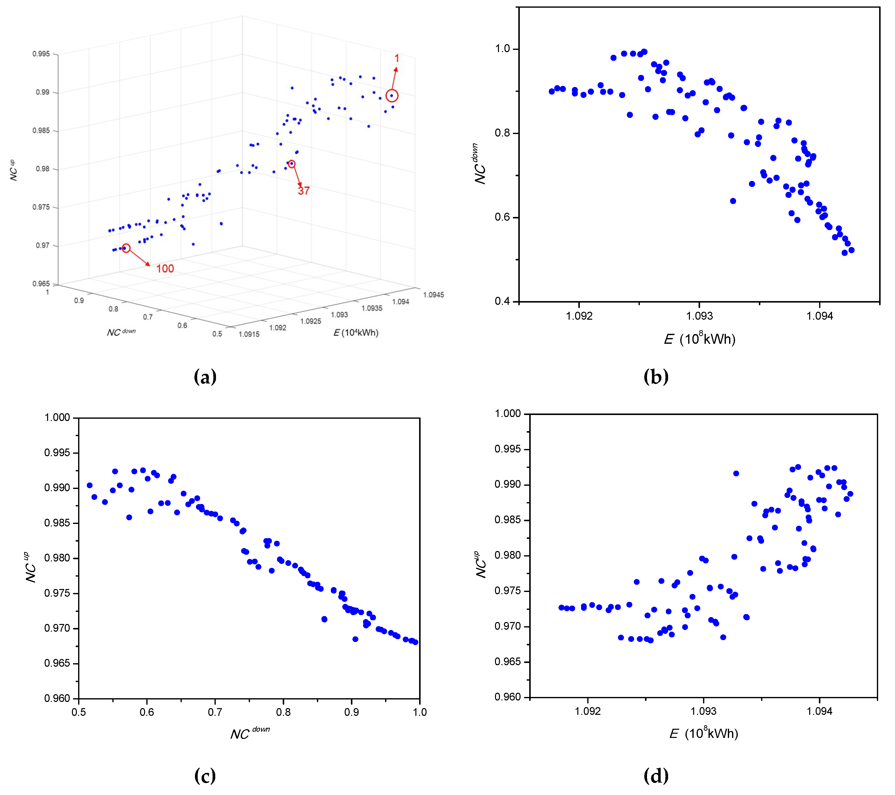
- (1)
- There is an obvious inverse relationship between the total power generation () and the downstream navigation capacity () from the results of Figure 10b. The larger the total power generation (), the smaller the downstream navigation capacity () in a day. The minimum value of is 0.52, and the maximum value is 0.99 with a growth of 90.38%, which varies greatly. At the same time, there is a drop of from the maximum value at 10,942.07 × 104 kWh to the minimum value at 10,925.44 × 104 kWh.
- (2)
- As shown in the Figure 10c, there is a certain inverse trend between the upstream navigation capacity () and the downstream navigation capacity (). When the upstream navigation capacity increases, the downstream navigation capacity declines. The minimum value of in all the schemes is 0.968, and the maximum value is 0.992 with a smaller growth compared to the change in .
- (3)
- Finally, it can be seen that the relationship between the total power generation () and the upstream navigation capacity () is not obvious shown in the Figure 10d. There is little interaction between these two elements.
5.4. Discussion
6. Conclusions
- (1)
- The proposed NCEM to evaluate the navigation capability is reasonable and effective, and can comprehensively analyze the influence of flow velocity and water level variation on navigation accurately.
- (2)
- The proposed multi-objective model can obtain a favorable Pareto frontier and explore the relationship between objectives. In the case study of the XJB reservoir, there is an obvious inverse relationship between power generation and the downstream navigation capacity. Also, the relationship between downstream navigation capacity and upstream navigation capability is inverse. However, there is little interaction between power generation and upstream navigation capability.
- (3)
- The results illustrate that the method and model are reasonable and effective, and also indicate that they can provide a series of favorable optimal operation schemes for the reservoir to obtain economic and navigational benefits.
Author Contributions
Funding
Acknowledgments
Conflicts of Interest
References
- Zhao, J.S.; Wang, Z.J.; Weng, W.B. Study on the holistic model for water resources system. Sci. China Ser. E-Eng. Mater. Sci. 2004, 47S, 72–89. [Google Scholar] [CrossRef]
- Cai, X.M.; McKinney, D.C.; Lasdon, L.S. Solving nonlinear water management models using a combined genetic algorithm and linear programming approach. Adv. Water Resour. 2001, 24, 667–676. [Google Scholar] [CrossRef]
- Wang, Y.; Zhou, J.; Mo, L.; Zhang, R.; Zhang, Y. Short-term hydrothermal generation scheduling using differential real-coded quantum-inspired evolutionary algorithm. Energy 2012, 44, 657–671. [Google Scholar] [CrossRef]
- Mo, L.; Lu, P.; Wang, C.; Zhou, J. Short-term hydro generation scheduling of Three Gorges-Gezhouba cascaded hydropower plants using hybrid MACS-ADE approach. Energy Convers. Manag. 2013, 76, 260–273. [Google Scholar] [CrossRef]
- Mahor, A.; Rangnekar, S. Short term generation scheduling of cascaded hydro electric system using novel self adaptive inertia weight PSO. Int. J. Electr. Power Energy Syst. 2012, 34, 1–9. [Google Scholar] [CrossRef]
- Barros, M.; Tsai, F.; Yang, S.L.; Lopes, J.; Yeh, W. Optimization of large-scale hydropower system operations. J. Water Resour. Plan. Manag. ASCE 2003, 129, 178–188. [Google Scholar] [CrossRef]
- Zhang, X.; Luo, J.; Sun, X.; Xie, J. Optimal reservoir flood operation using a decomposition-based multi-objective evolutionary algorithm. Eng. Optim. 2019, 51, 42–62. [Google Scholar] [CrossRef]
- Feng, Z.; Niu, W.; Zhou, J.; Cheng, C. Multi-objective operation optimization of a cascaded hydropower system. J. Water Resour. Plan. Manag. 2017, 143, 05017010. [Google Scholar] [CrossRef]
- Nilsson, O.; Sjelvgren, D. Hydro unit start-up costs and their impact on the short term scheduling strategies of Swedish power producers. IEEE Trans. Power Syst. 1997, 12, 38–43. [Google Scholar] [CrossRef]
- Cheng, C.; Liao, S.; Tang, Z.; Zhao, M. Comparison of particle swarm optimization and dynamic programming for large scale hydro unit load dispatch. Energy Convers. Manag. 2009, 50, 3007–3014. [Google Scholar] [CrossRef]
- Yuan, X.; Zhang, Y.; Wang, L.; Yuan, Y. An enhanced differential evolution algorithm for daily optimal hydro generation scheduling. Comput. Math. Appl. 2008, 55, 2458–2468. [Google Scholar] [CrossRef] [Green Version]
- Yuan, X.; Ji, B.; Chen, Z.; Chen, Z. A novel approach for economic dispatch of hydrothermal system via gravitational search algorithm. Appl. Math. Comput. 2014, 247, 535–546. [Google Scholar] [CrossRef]
- Castelletti, A.; Pianosi, F.; Restelli, M. A multiobjective reinforcement learning approach to water resources systems operation: Pareto frontier approximation in a single run. Water Resour. Res. 2013, 49, 3476–3486. [Google Scholar] [CrossRef] [Green Version]
- Wu, X.; Cheng, C.; Lund, J.R.; Niu, W.; Miao, S. Stochastic dynamic programming for hydropower reservoir operations with multiple local optima. J. Hydrol. 2018, 564, 712–722. [Google Scholar]
- Xie, M.; Zhou, J.; Li, C.; Lu, P. Daily generation scheduling of cascade hydro plants considering peak shaving constraints. J. Water Resour. Plan. Manag. 2016, 142, 04015072. [Google Scholar] [CrossRef]
- Kalumba, M.; Nyirenda, E. River flow availability for environmental flow allocation downstream of hydropower facilities in the Kafue Basin of Zambia. Phys. Chem. Earth 2017, 102, 21–30. [Google Scholar] [CrossRef]
- Shang, Y.; Li, X.; Gao, X.; Guo, Y.; Ye, Y.; Shang, L. Influence of daily regulation of a reservoir on downstream navigation. J. Hydrol. Eng. 2017, 22, 05017010. [Google Scholar] [CrossRef]
- Yang, Y.; Zhang, M.; Zhu, L.; Liu, W.; Han, J.; Yang, Y. Influence of large reservoir operation on water-levels and flows in reaches below dam: Case study of the Three Gorges Reservoir. Sci. Rep. 2017, 7, 15640. [Google Scholar] [CrossRef]
- Wagenpfeil, J.; Arnold, E.; Linke, H.; Sawodny, O. Modelling and optimized water management of artificial inland waterway systems. J. Hydroinformat. 2013, 15, 348–365. [Google Scholar] [CrossRef]
- Jia, T.; Zhou, J.; Liu, X. A daily power generation optimized operation method of hydropower stations with the navigation demands considered. MATEC Web Conf. 2018, 246, 01065. [Google Scholar] [CrossRef]
- Caris, A.; Limbourg, S.; Macharis, C.; van Lier, T.; Cools, M. Integration of inland waterway transport in the intermodal supply chain: A taxonomy of research challenges. J. Transp. Geogr. 2014, 41, 126–136. [Google Scholar] [CrossRef]
- Ceylan, H.; Bell, M.G.H. Genetic algorithm solution for the stochastic equilibrium transportation networks under congestion. Transp. Res. Part Methodol. 2005, 39, 169–185. [Google Scholar]
- Bugarski, V.; Bačkalić, T.; Kuzmanov, U. Fuzzy decision support system for ship lock control. Expert Syst. Appl. 2013, 40, 3953–3960. [Google Scholar] [CrossRef]
- Bierwirth, C.; Meisel, F. A survey of berth allocation and quay crane scheduling problems in container terminals. Eur. J. Oper. Res. 2010, 202, 615–627. [Google Scholar] [CrossRef]
- Ji, B.; Yuan, X.; Yuan, Y. Orthogonal design-based NSGA-III for the optimal lockage co-scheduling problem. IEEE Trans. Intell. Transp. Syst. 2017, 18, 2085–2095. [Google Scholar]
- Ji, B.; Yuan, X.; Yuan, Y.; Lei, X.; Fernando, T.; Lu, H.H. Exact and heuristic methods for optimizing lock-quay system in inland waterway. Eur. J. Oper. Res. 2019, 277, 740–755. [Google Scholar]
- Yuan, X.; Ji, B.; Yuan, Y.; Wu, X.; Zhang, X. Co-scheduling of lock and water–land transshipment for ships passing the dam. Appl. Soft Comput. 2016, 45, 150–162. [Google Scholar]
- Ackermann, T.; Loucks, D.P.; Schwanenberg, D.; Detering, M. Real-time modeling for navigation and hydropower in the River Mosel. J. Water Resour. Plan. Manag. ASCE 2000, 126, 298–303. [Google Scholar]
- Wang, J.; Zhang, Y. Short-Term optimal operation of hydropower reservoirs with unit commitment and navigation. J. Water Resour. Plan. Manag. ASCE 2012, 138, 3–12. [Google Scholar] [CrossRef]
- Ma, C. Fast optimal decision of short-term dispatch of Three Gorges and Gezhouba cascade hydropower stations with navigation demand considered. Syst. Eng. Theory Pract. 2013, 33, 1345–1350. (In Chinese) [Google Scholar]
- Liu, Y.; Qin, H.; Mo, L.; Wang, Y.; Chen, D.; Pang, S.; Yin, X. Hierarchical flood operation rules optimization using multi-objective cultured evolutionary algorithm based on decomposition. Water Resour. Manag. 2018, 33, 337–354. [Google Scholar] [CrossRef]
- Nithiarasu, P.; Zienkiewicz, O.C.; Sai, B.; Morgan, K.; Codina, R.; Vazquez, M. Shock capturing viscosities for the general fluid mechanics algorithm. Int. J. Numer. Methods Fluids 1998, 28, 1325–1353. [Google Scholar] [CrossRef]
- Casulli, V.; Walters, R.A. An unstructured grid, three-dimensional model based on the shallow water equations. Int. J. Numer. Methods Fluids 2000, 32, 331–348. [Google Scholar] [CrossRef]
- Erpicum, S.; Pirotton, M.; Archambeau, P.; Dewals, B.J. Two-dimensional depth-averaged finite volume model for unsteady turbulent flows. J. Hydraul. Res. 2014, 52, 148–150. [Google Scholar] [CrossRef]
- Kuiry, S.N.; Pramanik, K.; Sen, D. Finite volume model for shallow water equations with improved treatment of source terms. J. Hydraul. Eng. ASCE 2008, 134, 231–242. [Google Scholar] [CrossRef]
- Lu, W.L.; Chen, Z.Q. Study on navigational flow conditions of port areas and connection sections of navigation buildings. Southwest Highw. 2008. (In Chinese) [Google Scholar] [CrossRef]
- Feng, Y.; Zhou, J.; Mo, L.; Yuan, Z.; Zhang, P.; Wu, J.; Wang, C.; Wang, Y. Long-term hydropower generation of cascade reservoirs under future climate changes in Jinsha River in southwest China. Water 2018, 10, 235. [Google Scholar] [CrossRef]
- Wen, X.; Zhou, J.; He, Z.; Wang, C. Long-term scheduling of large-scale cascade hydropower stations using improved differential evolution algorithm. Water 2018, 10, 383. [Google Scholar] [CrossRef]
- Chang, L.; Chang, F. Multi-objective evolutionary algorithm for operating parallel reservoir system. J. Hydrol. 2009, 377, 12–20. [Google Scholar] [CrossRef]
- Zhao, T.T.G.; Zhao, J.S. Improved multiple-objective dynamic programming model for reservoir operation optimization. J. Hydroinformat. 2014, 16, 1142–1157. [Google Scholar] [CrossRef]
- Zitzler, E.; Laumanns, M.; Thiele, L. SPEA2: Improving the strength pareto evolutionary algorithm. ETH Zur. Res. Collect. 2001. [Google Scholar] [CrossRef]
- Deb, K.; Pratap, A.; Agarwal, S.; Meyarivan, T. A fast and elitist multiobjective genetic algorithm: NSGA-II. IEEE Trans. Evol. Comput. 2002, 6, 182–197. [Google Scholar] [CrossRef] [Green Version]
- Zhou, J.; Lu, P.; Li, Y.; Wang, C.; Yuan, L.; Mo, L. Short-term hydro-thermal-wind complementary scheduling considering uncertainty of wind power using an enhanced multi-objective bee colony optimization algorithm. Energy Convers. Manag. 2016, 123, 116–129. [Google Scholar] [CrossRef]
- Lai, X.; Li, C.; Zhang, N.; Zhou, J. A multi-objective artificial sheep algorithm. Neural Comput. Appl. 2018. [Google Scholar] [CrossRef]
- Wang, W.; Li, C.; Liao, X.; Qin, H. Study on unit commitment problem considering pumped storage and renewable energy via a novel binary artificial sheep algorithm. Appl. Energy 2017, 187, 612–626. [Google Scholar] [CrossRef]
- Li, C.; Wang, W.; Chen, D. Multi-objective complementary scheduling of hydro-thermal-RE power system via a multi-objective hybrid grey wolf optimizer. Energy 2019, 171, 241–255. [Google Scholar] [CrossRef]


| Characteristics of Water Level (m) | Installed Capacity/MW | Minimum Power/MW | Flow Velocity (m/s) | |||||
|---|---|---|---|---|---|---|---|---|
| Dead Water Level | The Normal Height | umax1 (m/s) | vmax2 (m/s) | |||||
| 370 | 380 | 6400 | 1800 | 12,000 | 1200 | 2.0 | 0.3 | 1.5 |
| Condition | Discharge | Working Turbines | UBL 1 | Simulation |
|---|---|---|---|---|
| 1 | Symmetric flow | All turbines | AC | Preliminary simulation and elaborate simulation |
| 2 | Asymmetric flow | Four left-bank turbines | AB | Asymmetric flow simulation |
| 3 | Asymmetric flow | Four right-bank turbines | BC | Asymmetric flow simulation |
| Model | Condition | UBC 1 | DBC 2 | u (m/s) 4 | v (m/s) 4 | UBL |
|---|---|---|---|---|---|---|
| Q (m3/s) 3 | Z (m) 3 | |||||
| Upstream | P1 | 9880 | 380 | 0.08–0.12 | 0.04–0.05 | —— |
| P2 | 9970 | 370 | 0.16–0.28 | 0.02–0.10 | —— | |
| Downstream | P3 | 1200 | 265.8 | 0.05–0.35 | 0.025–0.125 | AC |
| P4 | 12,000 | 277.25 | 0.50–2.00 | 0.3 (locally) | AC |
| No. | UBC | DBC | Dd | Cross-Sectional Water Level | ||||||||
|---|---|---|---|---|---|---|---|---|---|---|---|---|
| Qx | No. 10 | No. 11 | No. 12 | No. 13 | No. 14 | No. 15 | No. 16 | No. 17 | No. 18 | |||
| 1 | 1200 | 265.8 | 0 | 265.80 | 265.80 | 265.80 | 265.80 | 265.80 | 265.80 | 265.80 | 265.80 | 265.80 |
| 2 | 1700 | 266.7 | 0 | 266.72 | 266.72 | 266.72 | 266.72 | 266.72 | 266.72 | 266.72 | 266.72 | 266.72 |
| 3 | 2200 | 267.6 | 0 | 267.56 | 267.56 | 267.56 | 267.56 | 267.56 | 267.56 | 267.56 | 267.56 | 267.56 |
| 4 | 2700 | 268.3 | 0 | 268.29 | 268.29 | 268.29 | 268.29 | 268.29 | 268.29 | 268.29 | 268.29 | 268.29 |
| 5 | 3200 | 269.0 | 0 | 269.00 | 269.00 | 269.00 | 269.00 | 269.00 | 269.00 | 269.00 | 269.00 | 269.00 |
| 6 | 3700 | 269.6 | 0 | 269.63 | 269.63 | 269.63 | 269.63 | 269.63 | 269.63 | 269.63 | 269.63 | 269.63 |
| 7 | 4200 | 270.2 | 25 | 270.24 | 270.24 | 270.24 | 270.24 | 270.24 | 270.24 | 270.24 | 270.24 | 270.24 |
| 8 | 4700 | 270.8 | 28 | 270.82 | 270.82 | 270.82 | 270.82 | 270.82 | 270.82 | 270.82 | 270.82 | 270.82 |
| 9 | 5200 | 271.3 | 31 | 271.35 | 271.35 | 271.35 | 271.35 | 271.35 | 271.35 | 271.35 | 271.35 | 271.35 |
| 10 | 5700 | 271.8 | 34 | 271.84 | 271.84 | 271.84 | 271.84 | 271.84 | 271.84 | 271.84 | 271.84 | 271.84 |
| 11 | 6200 | 272.3 | 36 | 272.32 | 272.32 | 272.32 | 272.32 | 272.32 | 272.31 | 272.31 | 272.31 | 272.31 |
| 12 | 6700 | 272.8 | 37 | 272.77 | 272.77 | 272.77 | 272.77 | 272.77 | 272.77 | 272.76 | 272.76 | 272.75 |
| 13 | 7200 | 273.2 | 38 | 273.21 | 273.21 | 273.21 | 273.21 | 273.21 | 273.21 | 273.20 | 273.20 | 273.19 |
| 14 | 7700 | 273.6 | 40 | 273.64 | 273.64 | 273.64 | 273.64 | 273.64 | 273.64 | 273.63 | 273.63 | 273.62 |
| 15 | 8200 | 274.1 | 41 | 274.07 | 274.07 | 274.07 | 274.07 | 274.07 | 274.07 | 274.06 | 274.06 | 274.05 |
| 16 | 8700 | 274.5 | 42 | 274.49 | 274.49 | 274.49 | 274.49 | 274.49 | 274.49 | 274.48 | 274.48 | 274.47 |
| 17 | 9200 | 274.9 | 43 | 274.92 | 274.92 | 274.92 | 274.92 | 274.92 | 274.92 | 274.91 | 274.91 | 274.90 |
| 18 | 9700 | 275.3 | 43.5 | 275.34 | 275.34 | 275.34 | 275.34 | 275.34 | 275.34 | 275.33 | 275.32 | 275.31 |
| 19 | 10,200 | 275.8 | 43.6 | 275.77 | 275.77 | 275.77 | 275.77 | 275.77 | 275.77 | 275.76 | 275.75 | 275.74 |
| 20 | 10,700 | 276.2 | 43.7 | 276.19 | 276.19 | 276.19 | 276.19 | 276.19 | 276.19 | 276.18 | 276.17 | 276.16 |
| 21 | 11,200 | 276.6 | 43.8 | 276.60 | 276.60 | 276.60 | 276.60 | 276.60 | 276.59 | 276.59 | 276.58 | 276.57 |
| 22 | 11,700 | 277.0 | 43.9 | 277.02 | 277.02 | 277.02 | 277.02 | 277.02 | 277.01 | 277.01 | 277.00 | 276.98 |
| 23 | 12,000 | 277.3 | 44.5 | 277.27 | 277.27 | 277.27 | 277.27 | 277.27 | 277.26 | 277.26 | 277.25 | 277.23 |
| No. | UBC | DBC | Cross-Sectional Water Level | ||||||||
|---|---|---|---|---|---|---|---|---|---|---|---|
| I | No. 1 | No. 2 | No. 3 | No. 4 | No. 5 | No. 6 | No. 7 | No. 8 | No. 9 | ||
| 1 | 5000 | 380.0 | 380.03 | 380.03 | 380.02 | 380.02 | 380.02 | 380.01 | 380.01 | 380.01 | 380.00 |
| 2 | 5000 | 379.5 | 379.50 | 379.50 | 379.50 | 379.50 | 379.50 | 379.50 | 379.50 | 379.50 | 379.50 |
| 3 | 5000 | 379.0 | 379.00 | 379.00 | 379.00 | 379.00 | 379.00 | 379.00 | 379.00 | 379.00 | 379.00 |
| 4 | 5000 | 378.5 | 378.50 | 378.50 | 378.50 | 378.50 | 378.50 | 378.50 | 378.50 | 378.50 | 378.50 |
| 5 | 5000 | 378.0 | 378.00 | 378.00 | 378.00 | 378.00 | 378.00 | 378.00 | 378.00 | 378.00 | 378.00 |
| 6 | 5000 | 377.5 | 377.50 | 377.50 | 377.50 | 377.50 | 377.50 | 377.50 | 377.50 | 377.50 | 377.50 |
| 7 | 5000 | 377.0 | 377.00 | 377.00 | 377.00 | 377.00 | 377.00 | 377.00 | 377.00 | 377.00 | 377.00 |
| 8 | 5000 | 376.5 | 376.50 | 376.50 | 376.50 | 376.50 | 376.50 | 376.50 | 376.50 | 376.50 | 376.50 |
| 9 | 5000 | 376.0 | 376.00 | 376.00 | 376.00 | 376.00 | 376.00 | 376.00 | 376.00 | 376.00 | 376.00 |
| 10 | 5000 | 375.5 | 375.50 | 375.50 | 375.50 | 375.50 | 375.50 | 375.50 | 375.50 | 375.50 | 375.50 |
| 11 | 5000 | 375.0 | 375.00 | 375.00 | 375.00 | 375.00 | 375.00 | 375.00 | 375.00 | 375.00 | 375.00 |
| 12 | 5000 | 374.5 | 374.50 | 374.50 | 374.50 | 374.50 | 374.50 | 374.50 | 374.50 | 374.50 | 374.50 |
| 13 | 5000 | 374.0 | 374.00 | 374.00 | 374.00 | 374.00 | 374.00 | 374.00 | 374.00 | 374.00 | 374.00 |
| 14 | 5000 | 373.5 | 373.50 | 373.50 | 373.50 | 373.50 | 373.50 | 373.50 | 373.50 | 373.50 | 373.50 |
| 15 | 5000 | 373.0 | 373.00 | 373.00 | 373.00 | 373.00 | 373.00 | 373.00 | 373.00 | 373.00 | 373.00 |
| 16 | 5000 | 372.5 | 372.50 | 372.50 | 372.50 | 372.50 | 372.50 | 372.50 | 372.50 | 372.50 | 372.50 |
| 17 | 5000 | 372.0 | 372.00 | 372.00 | 372.00 | 372.00 | 372.00 | 372.00 | 372.00 | 372.00 | 372.00 |
| 18 | 5000 | 371.5 | 371.50 | 371.50 | 371.50 | 371.50 | 371.50 | 371.50 | 371.50 | 371.50 | 371.50 |
| 19 | 5000 | 371.0 | 371.00 | 371.00 | 371.00 | 371.00 | 371.00 | 371.00 | 371.00 | 371.00 | 371.00 |
| 20 | 5000 | 370.5 | 370.50 | 370.50 | 370.50 | 370.50 | 370.50 | 370.50 | 370.50 | 370.50 | 370.50 |
| 21 | 5000 | 370.0 | 370.00 | 370.00 | 370.00 | 370.00 | 370.00 | 370.00 | 370.00 | 370.00 | 370.00 |
| Scheme | (104 kWh) | Scheme | (104 kWh) | ||||
|---|---|---|---|---|---|---|---|
| 1 | 10,942.07743 | 0.516103 | 0.990381 | 40 | 10,934.87 | 0.775069 | 0.982459 |
| 2 | 10,942.65972 | 0.522835 | 0.988732 | 41 | 10,938.68 | 0.776607 | 0.981775 |
| 3 | 10,942.33743 | 0.538384 | 0.988012 | 42 | 10,933.95 | 0.778997 | 0.982459 |
| 4 | 10,942.11842 | 0.550021 | 0.989657 | 43 | 10,937.91 | 0.783004 | 0.978221 |
| 5 | 10,941.27857 | 0.553263 | 0.992386 | 44 | 10,934.97 | 0.790506 | 0.982092 |
| … | … | … | … | … | … | … | … |
| 35 | 10,939.44119 | 0.742237 | 0.981028 | 96 | 10,922.86 | 0.979242 | 0.968444 |
| 36 | 10,939.48026 | 0.745708 | 0.980875 | 97 | 10,925.08 | 0.987635 | 0.96826 |
| 37 | 10,938.9987 | 0.750805 | 0.979485 | 98 | 10,924.49 | 0.989242 | 0.968253 |
| 38 | 10,938.77714 | 0.758043 | 0.979526 | 99 | 10,923.75 | 0.989259 | 0.968254 |
| 39 | 10,938.71673 | 0.763488 | 0.978766 | 100 | 10,925.44 | 0.99352 | 0.968062 |
© 2019 by the authors. Licensee MDPI, Basel, Switzerland. This article is an open access article distributed under the terms and conditions of the Creative Commons Attribution (CC BY) license (http://creativecommons.org/licenses/by/4.0/).
Share and Cite
Jia, T.; Qin, H.; Yan, D.; Zhang, Z.; Liu, B.; Li, C.; Wang, J.; Zhou, J. Short-Term Multi-Objective Optimal Operation of Reservoirs to Maximize the Benefits of Hydropower and Navigation. Water 2019, 11, 1272. https://doi.org/10.3390/w11061272
Jia T, Qin H, Yan D, Zhang Z, Liu B, Li C, Wang J, Zhou J. Short-Term Multi-Objective Optimal Operation of Reservoirs to Maximize the Benefits of Hydropower and Navigation. Water. 2019; 11(6):1272. https://doi.org/10.3390/w11061272
Chicago/Turabian StyleJia, Tianlong, Hui Qin, Dong Yan, Zhendong Zhang, Bin Liu, Chaoshun Li, Jinwen Wang, and Jianzhong Zhou. 2019. "Short-Term Multi-Objective Optimal Operation of Reservoirs to Maximize the Benefits of Hydropower and Navigation" Water 11, no. 6: 1272. https://doi.org/10.3390/w11061272