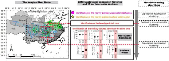
Using Real-Time Data and Unsupervised Machine Learning Techniques to Study Large-Scale Spatio–Temporal Characteristics of Wastewater Discharges and their Influence on Surface Water Quality in the Yangtze River Basin

Abstract

Most worldwide industrial wastewater, including in China, is still directly discharged to aquatic environments without adequate treatment. Because of a lack of data and few methods, the relationships between pollutants discharged in wastewater and those in surface water have not been fully revealed and unsupervised machine learning techniques, such as clustering algorithms, have been neglected in related research fields. In this study, real-time monitoring data for chemical oxygen demand (COD), ammonia nitrogen (NH₃-N), pH, and dissolved oxygen in the wastewater discharged from 2213 factories and in the surface water at 18 monitoring sections (sites) in 7 administrative regions in the Yangtze River Basin from 2016 to 2017 were collected and analyzed by the partitioning around medoids (PAM) and expectation–maximization (EM) clustering algorithms, Welch t-test, Wilcoxon test, and Spearman correlation. The results showed that compared with the spatial cluster comprising unpolluted sites, the spatial cluster comprised heavily polluted sites where more wastewater was discharged had relatively high COD (>100 mg L⁻¹) and NH₃-N (>6 mg L⁻¹) concentrations and relatively low pH (<6) from 15 industrial classes that respected the different discharge limits outlined in the pollutant discharge standards. The results also showed that the economic activities generating wastewater and the geographical distribution of the heavily polluted wastewater changed from 2016 to 2017, such that the concentration ranges of pollutants in discharges widened and the contributions from some emerging enterprises became more important. The correlations between the quality of the wastewater and the surface water strengthened as the whole-year data sets were reduced to the heavily polluted periods by the EM clustering and water quality evaluation. This study demonstrates how unsupervised machine learning algorithms play an objective and effective role in data mining real-time monitoring information and highlighting spatio–temporal relationships between pollutants in wastewater discharges and surface water to support scientific water resource management.

1. Introduction

Except in the most highly developed countries, most worldwide wastewater is treated inadequately before being released to the environment, with negative consequences for human health, economic productivity, the quality of freshwater resources, and ecosystems. In many cases, a large volume of the wastewater that is legally discharged to decaying and/or poorly-maintained sewerage networks, both combined and separate, never actually reaches a treatment plant. Much is lost en route because of broken pipes, or ends up in surface water drains, and may pollute watercourses [1]. In China, factories prefer to be located beside rivers so that they have easy access to water and the generated wastewater can be easily discharged to the water environment, mostly without adequate treatment. For example, more than 400,000 chemical enterprises, nearly half of the country’s total, are located along the middle and lower reaches of the Yangtze River [2]. In 2014, China implemented a national strategy to develop the Yangtze River Economic Belt, which accounts for more than 40% of both the national population and GDP and stretches from Yunnan Province in the southwest of China to Shanghai in the east, to boost development in riverside regions and provide new stimuli for China’s slowing economy and, at the same time, to restore and protect the environment [2,3]. Based on the assumption that the enterprises along the river are a major source of pollution, the strategy required that, to protect the river environment, all the petrochemical enterprises and sewage outlets in environmentally-sensitive areas along the Yangtze River should be closed by the end of June 2018 and that all illegal petrochemical enterprises that had high pollutant emissions and were within a 1-km radius of the Yangtze River should be closed by the end of 2018 [4]. Because of a lack of data and few methods, however, there is no clear picture of how much these enterprises contributed to the river pollution or about how the pollutants in wastewater discharges from specific economic activities are related to the surface water quality in the same region.

Traditionally, when modelling water environments, urban water systems and river basins have been treated separately [5], and factory wastewater has generally been considered in urban systems and not in rural river basins [6]. Because of a lack of spatial and temporal data, the relationships between point and non-point pollutant sources and water quality have only been studied at the microscale in the past [7,8]. Luckily, at present, more data are available and data-driven approaches and statistical (or numerical) models are now playing an increasingly important role in water management, so that environmental decision support systems (EDSSs) are more reliable and are capable of coping with real-world environmental systems [9,10,11]. Numerous researchers have analyzed real-time data to support the management of urban water and water supplies in developed countries [12,13,14,15], but this approach has not often been used to manage large rural watersheds or wastewater [16,17].

Clustering algorithms, as established unsupervised machine learning models, have been used to analyze data from a wide range of disciplines, such as gene expression data in biology and stock market financial data [18,19], yet have been rarely applied to the water environment due to the lack of data [11,20,21,22,23]. The partition-based, hierarchical, and density-based algorithms are all popular spatial clustering methods [24]. From the partition-based spatial clustering algorithms, the partitioning around medoids (PAM) algorithm uses a greedy search, which is faster than an exhaustive search, and is more robust to noise and outliers than k-Means because it minimizes a sum of pairwise dissimilarities instead of the sum of squared Euclidean distances. Therefore, PAM is an ideal spatial clustering technique for geographical data mining [25]. The expectation–maximization (EM) and k-means algorithms belong to the top 10 data mining algorithms identified by the IEEE International Conference on Data Mining (ICDM) in December 2006 [26] and have been increasingly popular in machine learning [27]. As the k-means algorithm has limitations, including that it will falter whenever the data is not well described by reasonably separated spherical balls and it has difficulties in handling noisy data, or outliers [21,26], the k-means algorithm seems ill suited to research on environmental pollution with abnormally high concentrations of pollutants, which might be highly informative outliers. Moreover, the EM algorithm assigns each data object to a cluster according to the mean of the feature values in that cluster. Its steps of calculation and assignment repeat iteratively until the objective function obtains the required precision [28]. Low-dimensional data can be analyzed successfully with the EM clustering algorithm, and this approach is particularly useful when the only data available for training a probabilistic model are incomplete [11,18,28,29]. Therefore, the EM algorithm, as an improvement of k-means, is an ideal unsupervised machine learning method for clustering pollution conditions [30,31] and has been proven as objective and efficient in evaluating surface water quality of the Yangtze river in China in our earlier study [11]. Wastewater generating factories are important potential pollution point sources of surface water in rivers and their effects on bad surface water quality need further study. To our knowledge, however, these source–sink relationship studies on water environment management in large river basins have not been studied by using unsupervised machine learning techniques yet.

In this study, real-time monitoring data for COD, NH₃-N, and pH in wastewater discharges from seven administrative regions (ARs, they are provinces or municipalities of China) in the Yangtze River Basin (YRB); geographical and administrative data; information about the wastewater-generating factories in the Yangtze River Basin (YRB); and real-time data for COD, NH₃-N, pH, and DO from 18 surface water sections (sites) in the YRB that are part of the national monitoring program were obtained for 2016 and 2017. The PAM and EM clustering algorithms were used to (a) spatially divide the YRB wastewater-generating factories and YRB monitoring sites, (b) identify sites in the YRB that were heavily polluted and unpolluted and examine the differences in sources of pollutants at these sites, (c) identify heavily polluted and unpolluted wastewater and economic activities in the YRB, and (d) explore the spatio–temporal characteristics of pollutants in industrial discharges and surface water. The aims of the study were to develop unsupervised machine learning techniques and numeric methods that could be applied to real-time data about wastewater and the water environment to determine how industrial point sources influence surface water in the same region and to support and improve water resource management to be more objective and reliable.

2. Material and Methods

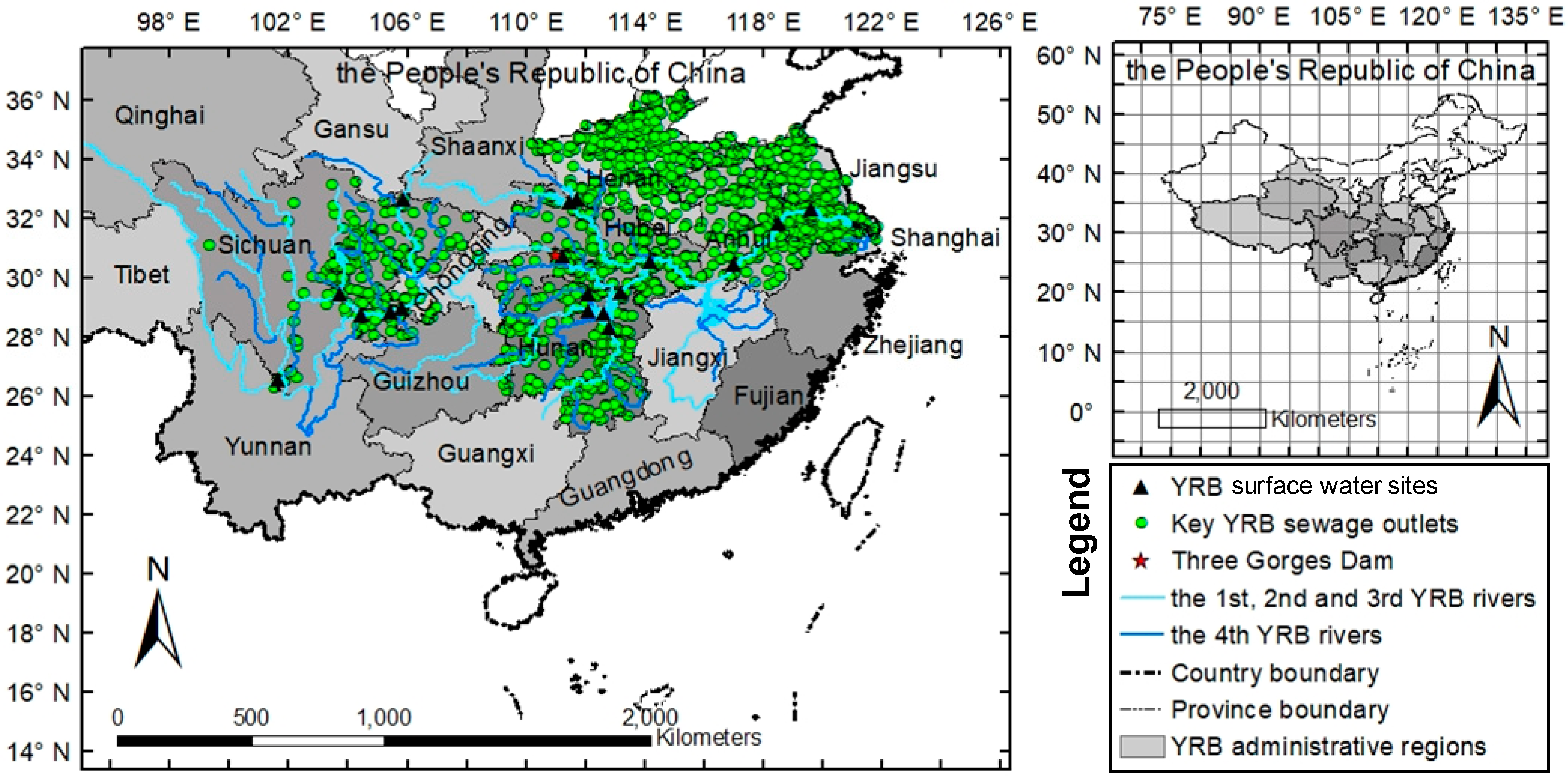
2.1. Study Area, Monitoring Surface Water Sites, and Monitored Sewage Outlets

The Yangtze River, which is 6380 km long, is the longest river in Asia and the third-longest in the world. The river flows entirely within one country, drains one-fifth of the land area of the People’s Republic of China, and its river basin is home to nearly one-third of the country’s population [32,33]. There are 21 surface water sections (sites) that are part of a national monitoring program with real-time monitoring data in the Yangtze River Basin (YRB), but only 18 sites are located in the 7 ARs—Sichuan Province (SC), Chongqing Municipality (CQ), Hunan Province (HuN), Hubei Province (HB), Henan Province (HeN), Anhui Province (AH), and Jiangsu Province (JS)—that published monitoring data of pollutants in wastewater discharges from sewage outlets of industrial factories online in 2016 and 2017 (Figure 1, Table S1). Therefore, the 7 ARs were chosen to study their wastewater generating factories where the Yangtze River mainly goes through. In 2016 and 2017, there were 2386 monitored sewage outlets from the 2213 factories (some wastewater-generating factories each had more than one sewage outlet) of the 7 ARs with monitoring wastewater discharge data published online (Figure 1, Table S1). The sewage outlets and their factories were called the YRB sewage outlets and the YRB wastewater-generating factories separately for succinct expression with their incomplete river basin information. These factories were the key pollution sources as part of a national monitoring network according to their big wastewater discharge loads above the limit of 500 thousand ton year⁻¹ in the screening principles released by the State Environmental Protection Administration, China’s top environmental watchdog [34].

2.2. Wastewater-Generating Economic Activities in the YRB in 2016 and 2017

Chinese economic activities are classified using the “Industrial classification for national economic activities in China” (No. GB/T 4754-2017, the IC document) [35]. This IC document corresponds with the UN International standard industrial classification of all economic activities (the ISIC document) [36]. The IC and the ISIC documents classify economic data according to the type of activity carried out by an economic unit and define an industry as a set of production units engaged primarily in the same or similar productive economic activities. Their classifications mainly facilitate the collection and reporting of statistics about industrial activities in different categories. There were 2213 factories belonging to 41 industrial classes in the IC document and wastewater discharge data was published online from the 6 YRB ARs (CQ, HuN, HB, HeN, AH and JS) in 2016 (1700 factories) and from the 7 YRB ARs, including SC, in 2017 (2178 factories) (Figure S1, Table S2).

2.3. Monitoring Methods and Data Sources

Monitoring stations with automatic analyzers that provide real-time water quality data have been established across China in recent years to support watershed management and help control pollutant discharges [37,38]. The real-time data generally comprise four indicators of water quality, namely pH, dissolved oxygen (DO), permanganate index for chemical oxygen demand (COD_Mn), and ammonia nitrogen (NH₃-N), and other parameters are not included in the real-time data sets published online. Real-time data about the sources of pollutant discharges are released on internet platforms, which means that regulations are enforced transparently [34]. Data for water quality indicators, such as chemical oxygen demand (COD determined by the potassium dichromate method, also called COD_Cr), NH₃-N, pH, and other industry-specific pollutants, are monitored automatically by companies that generate wastewater and have been increasingly published online since 2015 in China. Only COD, NH₃-N, and pH are monitored in real time in all economic activities.

For surface water at the YRB sites, the monitoring data of COD (COD_Mn), NH₃-N, DO, and pH were collected from the weekly reports on the automatic monitoring data of national water quality published online (http://www.cnemc.cn/sssj/szzdjczb/) and the real-time data were collected from the online open system of real-time automatic monitoring data of national surface water quality (http://123.127.175.45:8082/) [39,40]. The monitoring frequency of one real-time sample was four hours.

For wastewater discharged from the YRB sewage outlets, the monitoring data of COD (COD_Cr), NH₃-N, and pH and the geographical, administrative, and industrial information of their wastewater-generating factories were collected from online open monitoring information planforms of the specially monitored enterprises of the 7 ARs. The monitoring data publishing frequencies of one sample included one or more times per two hours, one or more times per day, one or more times per week, and one or more times per month.

2.4. Models and Algorithms

2.4.1. Clustering Algorithms

The partitioning around medoids (PAM) clustering algorithm, also simply referred to as k-medoids, is the most common realization of k-medoid clustering [41]. The k-medoids clustering is very similar to k-means, and the major difference between them is that while a cluster is represented with its center in the k-means algorithm, it is represented with the object closest to the center of the cluster in the k-medoids clustering. The k-medoids clustering is more robust than k-means in the presence of outliers. To deal with the high run time cost of PAM, the CLARA algorithm (Clustering large applications) is used to enhance PAM by drawing multiple samples of data, applying PAM on each sample, and then returning the best clustering [41,42]. This enhanced PAM method was used to classify the spatial distribution of sites and wastewater-generating factories as point sources with their latitudes and longitudes as input data. The number of clusters was estimated by the optimum average silhouette width (asw) [43].

The expectation–maximization (EM) clustering algorithm is an iterative method to find the maximum likelihood or maximum a posteriori (MAP) estimates of parameters in statistical models depending on the unobserved latent variables [29]. An integrated approach to finite Gaussian mixture modelling (GMM) [44], with functions that combine model-based hierarchical clustering, the EM algorithm for mixture estimation, and several tools for model selection (EM clustering for short), was used and proposed by different names based on different input data sets in this study (Table S3). The GMM assumes a (multivariate) Gaussian distribution for each component, i.e., f_k(x; θ_k) ∼ N(µ_k, Σ_k). Thus, clusters are ellipsoidal, centered at the mean vector, µ_k, and with other geometric features, such as volume, shape, and orientation, determined by the covariance matrix, Σ_k. Parsimonious parameterizations of the covariance matrices can be obtained by means of an Eigen-decomposition of the form, Σ_k = λ_kD_kA_kD_k^T, where λ_k is a scalar controlling the volume of the ellipsoid, A_k is a diagonal matrix specifying the shape of the density contours with det(A_k) = 1, and D_k is an orthogonal matrix which determines the orientation of the corresponding ellipsoid. In the multivariate setting, the volume, shape, and orientation of the covariances can be constrained to be equal or variable across groups. Thus, 18 possible models with different geometric characteristics can be specified. The Bayesian information criterion (BIC) was selected as the model identification criteria [44]. The Mclust model with the covariance parameterization and a specific number (k) of mixing components which had the highest BIC value was identified as the best EM model and the k value was identified as the best number of clusters (Table S3). The YRB sites were clustered based on the yearly means of COD, NH₃-N, pH, and DO in surface water in 2016 (EM_SA Method) and 2017 (EM_SB Method). The EM_SA Method was the same as the EM_Y Method in our previous study [11]. The YRB sewage outlets were clustered based on the yearly means of COD, NH₃-N, and pH in wastewater discharges and the EM models used were named EM_A Method (COD, NH₃-N, and pH data in 2016 were input), EM_B Method (COD and NH₃-N data in 2016 were input), EM_C Method (COD, NH₃-N, and pH data in 2017 were input), or EM_D Method (COD and NH₃-N data in 2017 were input). Wastewater discharge weeks were also clustered based on weekly means of COD, NH₃-N, and pH in wastewater in a specific cluster of sewage outlets from the clustering results above-mentioned and it was named the EM_E Method for the 2016 data and named the EM_F Method for the 2017 data. The monitoring weeks of surface water quality at a specific YRB site was lastly clustered based on weekly means of COD, NH₃-N, and DO in the surface water and it was named the EM_SC Method for the 2016 data and the EM_SD Method for the 2017 data.

2.4.2. Significance Tests with Confidence Intervals

As nonparametric statistical methods, the Student’s t-test with the Welch approximation to the degrees of freedom to estimate the variance (Welch t-test) and Wilcoxon rank sum and signed rank test (Wilcoxon test, also known as the Mann–Whitney test) are robust two-sample tests for general data sets, including data sets with unequal sample sizes and nonhomogeneity of variances [45]. Considering the data sets in our study had unequal sample sizes and nonhomogeneity of variances, the Welch t-test and Wilcoxon test were separately performed to test the difference significance between annual pollutant means and medians in the wastewater discharged from all the YRB sewage outlets and in the surface water at the 18 YRB sites in 2016 and 2017 in different clusters and to evaluate the clustering results. Our null hypothesis is that the annual means or medians of pollutants in different clusters are statistically equal. Confidence intervals of the Welch t-test and Wilcoxon test were offered for more information.

2.4.3. Correlation Analyses

Considering that the data sets in our study did not statistically obey normal distribution by the normal distribution test, correlation analyses between the daily means of the four monitoring indicators in surface water and wastewater were performed by the Spearman correlation to study their temporal relationships. Significance levels were reported as non-significant (p > 0.05) and significant (p < 0.05).

2.4.4. Software Application

The models and algorithms above were done and visualized and standard deviations (SDs) and coefficient of variation (CVs) were calculated by the Microsoft Excel 2016 and the RStudio (Version 1.0.153 with R 3.4.1, RStudio, Boston, MA, USA) and the geographical distributions were visualized by the ArcMap 10.2.2 (Esri, Redlands, CA, USA).

3. Results and Discussion

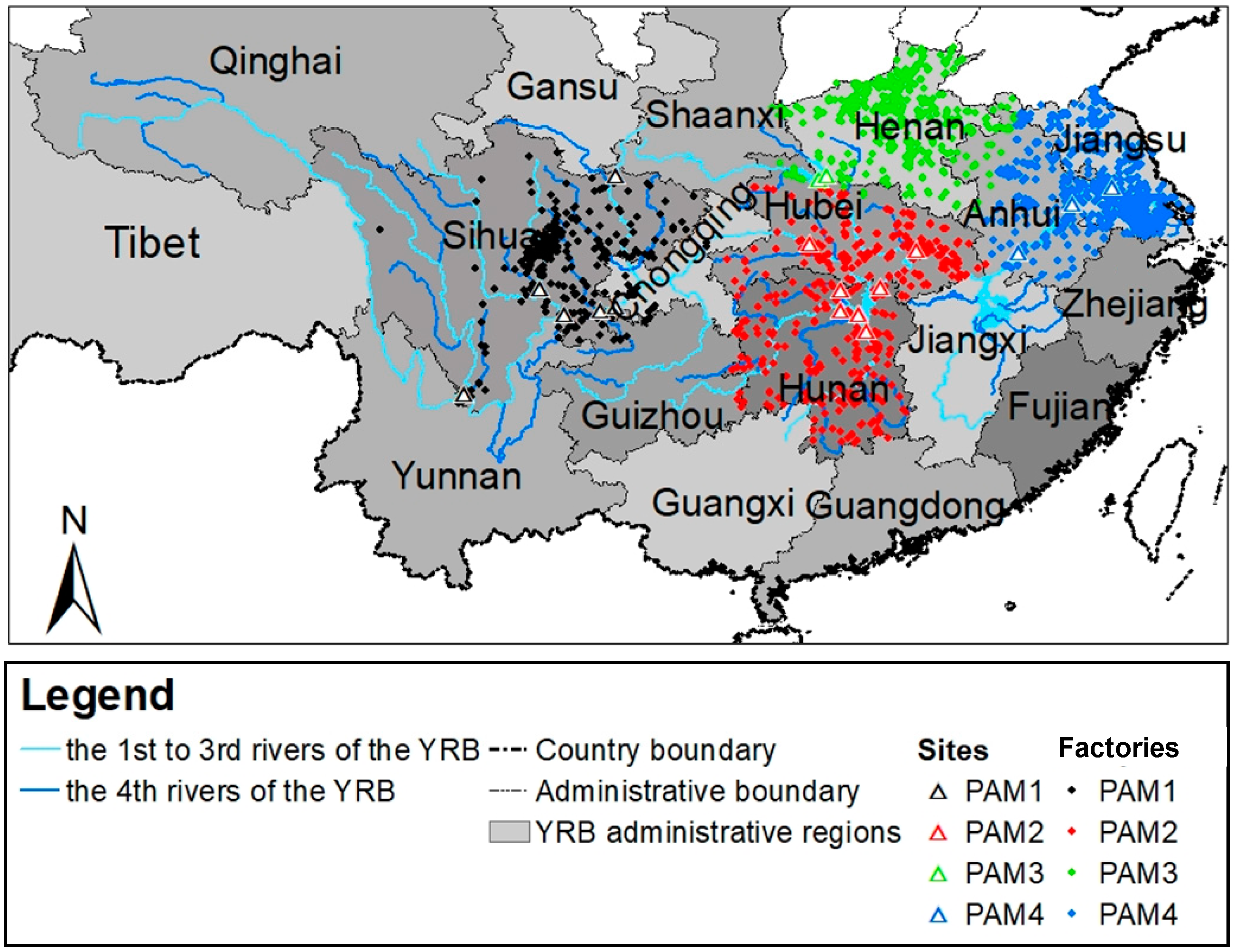
3.1. Spatial Zoning of the Wastewater-Generating Factories and the Surface Water Sites in the YRB Using the PAM Clustering

The 18 surface water quality sites and the 2213 wastewater-generating factories (occupying 2386 monitored sewage outlets) in the YRB were classified spatially into four PAM clusters (Figure 2, Table S4), based on their latitudes and longitudes and the number of clusters estimated by the optimum average silhouette width (asw = 0.6154, Table S3). Wastewater-generating factories and surface water sites in SC, CQ, HuN, HeN, AH, and JS ARs were mainly in the same spatial PAM clusters; HB was split between two PAM clusters, with 302 factories and 2 sites (HB1 and HB3) in PAM2 and 20 factories and 1 site (HB2) in PAM3 (Table S4). The spatial clusters were generally consistent with the provincial boundaries. Apart from the HuB2 site and several factories in AH, HB, and JS, surface water sections and wastewater-generating factories in the same AR were generally clustered in the same PAM cluster.

The latitudes and longitudes of the YRB surface water sites and YRB wastewater discharges were also clustered by hierarchical and DBSCAN (Density-based spatial clustering of applications with noise) algorithms besides the PAM method. The results showed that only the PAM method returned with consistent clusters and was proven to be a robust spatial clustering method for a huge dataset. The PAM clustering has also been researched as a robust method before and compared with other spatial clustering methods, such as k-means and DBSCAN [46]. Sewage outlets from all wastewater-generating factories through the whole administrative region of each province or municipality in the YRB were considered together, because the information published online about river basins and wastewater discharge regulations was either limited or unclear (see online open monitoring information platforms of the specially monitored enterprises of the 7 ARs). Factories that discharge wastewater are supervised together at the provincial level in China and wastewater discharged within a specific province needs to be analyzed together, regardless of whether it is clearly indicated in the YRB or not. Therefore, the PAM clustering, as a robust spatial clustering algorithm for big data, provides an objective method for spatial zoning the source-sink of pollutants in the water system of a large river basin under unsupervised conditions. The pollutant concentrations and water quality of the wastewater discharged and surface water in the same or different spatial PAM clusters were compared and the spatial distributions of heavily polluted wastewater discharges and surface water monitoring sites were also examined below.

3.2. Identification of Heavily Polluted and Unpolluted Wastewater and Surface Water in the YRB Using EM Clustering

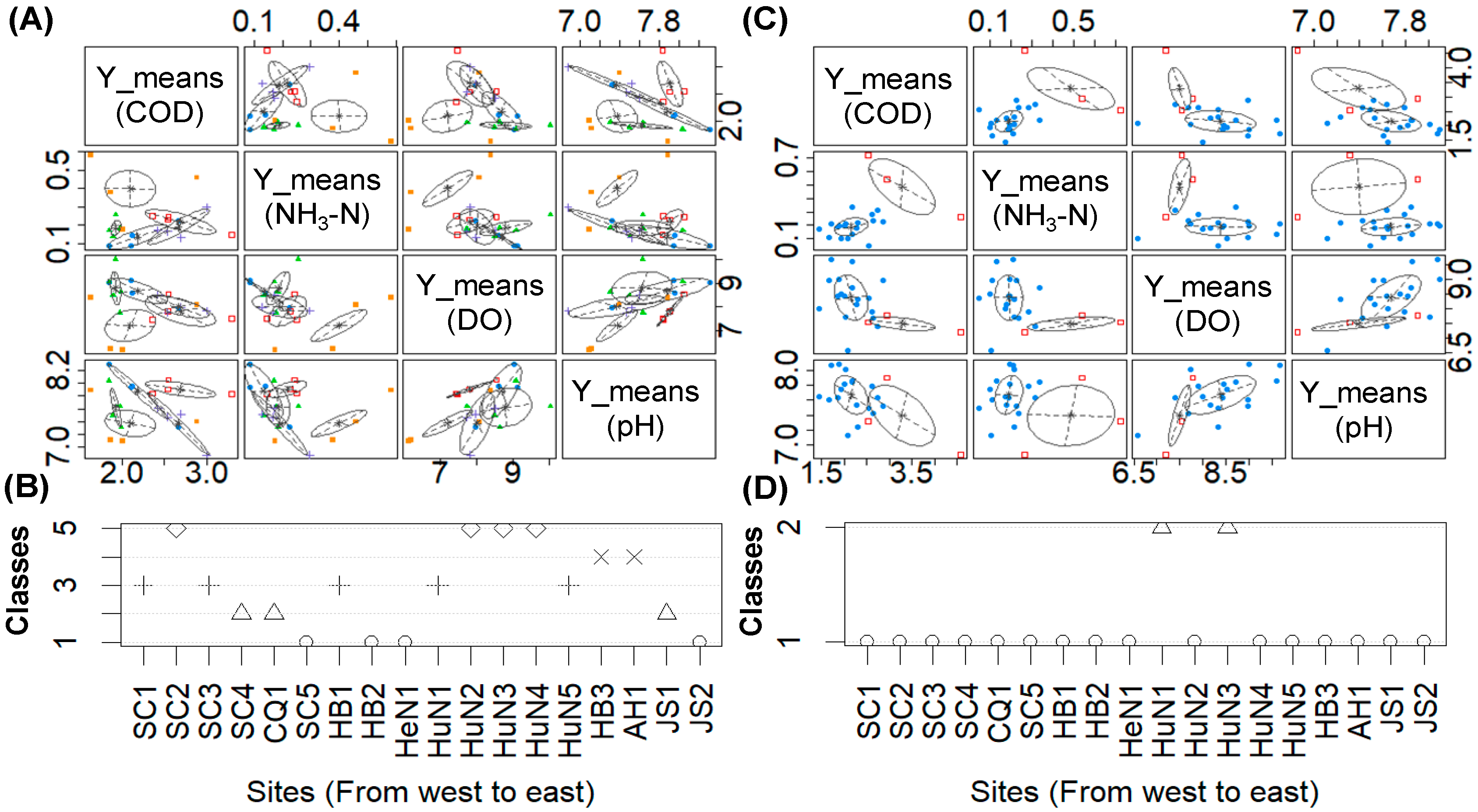
3.2.1. Identification of Heavily Polluted and Unpolluted Surface Water Sections in the YRB Using EM Clustering and Weekly Water Quality Data

Using the yearly means of COD, NH₃-N, DO, and pH for 2016 (Figure 3A,B, Table S5), the 18 sites were classified into 5 EM algorithm classes, namely EM1, EM2, EM3, EM4, and EM5, by the Mclust EEV (ellipsoidal, equal volume, and shape) model (EM_SA, Table S3). Class EM_SA_1 contained sites that had relatively low annual average concentrations of NH₃-N and relatively high annual average DO concentrations, including SC5, HB2, HeN1, and JS2. Class EM_SA_5 comprised sites that had relatively high annual averages of NH₃-N and relatively low annual averages of DO, including SC2, HuN2, HuN3, and HuN4. Using the yearly means of the four monitoring indicators in 2017 (Figure 3C,D, Table S5), the 18 sites were classified into two EM algorithm classes, EM1 and EM2, by Mclust EEV (EM_SB, Table S3). Class EM_SB_2 included HuN1 and HuN3 and had relatively high annual average COD and NH₃-N concentrations and relatively low annual average DO concentrations.

Some HuN sites belonged to the same spatial PAM cluster (PAM2) and the same EM cluster (EM5 in 2016 and EM2 in 2017) and had relatively low unpolluted weekly percentages. The HB2 and HeN1 sites belonged to the same spatial PAM cluster (PAM3) and the same EM cluster (EM1 in 2016 and 2017) and had weeks that were 100% unpolluted in both 2016 and 2017. Therefore, the HuN3 site, which had relatively poor water quality in both 2016 and 2017, was identified as heavily polluted (the HPS site) and HuB2 and HeN1, with relatively good water quality, were identified as unpolluted (the UPS sites). The HuB2 and HeN1 sites are in Danjiangkou Reservoir (Table S1), which is the main water source of the middle route of the South-to-North Water Diversion Project (MR-SNWDP) and supplies water to Beijing, Tianjin, and more than 130 other cities in northern China. Therefore, the water quality in the Danjiangkou Reservoir is extremely important for the safety of the drinking water in those cities [47]. The surface water quality was good through 2016 and 2017, thanks to the increased attention given to environment protection since around 2014 [48,49].

Similarly, results from hierarchical clustering with the Ward.D method (Figure S2) showed that the HuN3 site was clustered in heavily polluted sites and HuB2 and HeN1 were clustered in the unpolluted sites. The water quality assessments also showed that HuN had more sites and weeks with polluted water quality (lower than the national polluted standard limits [11]) than the other ARs both in 2016 and 2017 (the lowest unpolluted week percentages were 75.5% at the HuN4 site in 2016 and 90.6% at the HuN3 site in 2017) and the HuB2 and HeN1 sites had no polluted weeks either in 2016 or 2017 (Figure S3, Table S5). Therefore, it is reasonable to identify HuN3 as the heavily polluted site and HuB2 and HeN1 as unpolluted sites. Overall, the EM clustering (combine the EM algorithm with model-based hierarchical clustering) plays an efficient role in water quality classifications and pollution identification under unsupervised conditions, offers a good clustering choice in the visualization and understanding of the pollution distribution of surface water, and gives a feasible replacement of k-means [21], which has also been proven as efficient before [11].

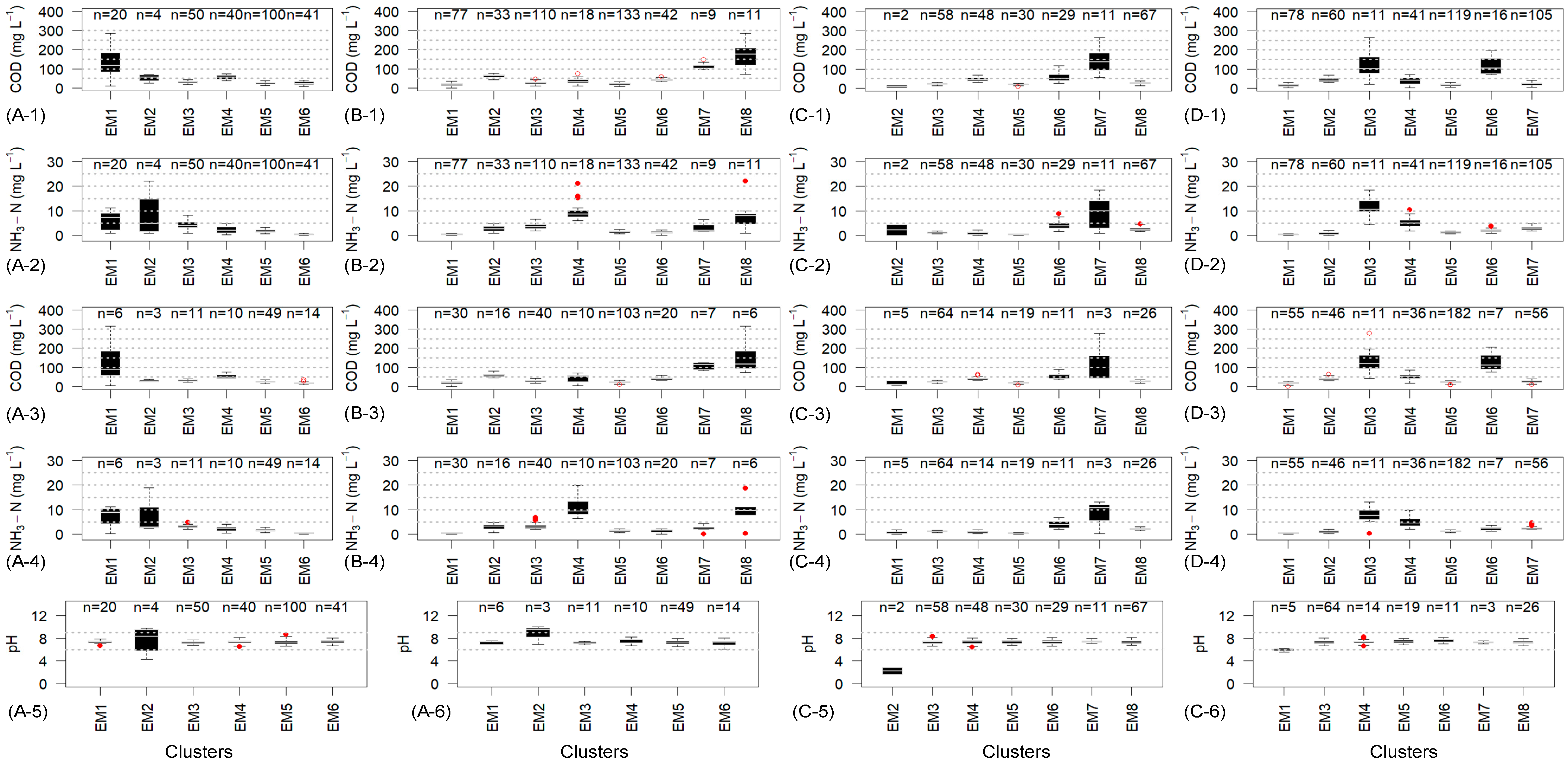
3.2.2. Identification of Heavily Polluted and Unpolluted Wastewater Discharges in the YRB Using EM Clustering

The EM_A method classified the YRB sewage outlets into six clusters, EM1 to EM6, based on the yearly means of COD, NH₃-N, and pH in the wastewater discharges in 2016 by Mclust VVI (diagonal, varying volume, and shape) model (Figure 4A, Table S3). Cluster EM_A_1 represented the sewage outlets with high COD (with median values exceeding 100 mg L⁻¹, the same below) and NH₃-N (greater than 6 mg L⁻¹) concentrations while Cluster EM_A_2 represented those with pH values below 6 or greater than 9. The EM_B method classified the sewage outlets into eight clusters, EM1 to EM8, based on the yearly means of COD and NH₃-N in 2016 by the Mclust VVI model (Figure 4B, Table S3). Cluster EM_B_8 represented the outlets with high COD (greater than 170 mg L⁻¹) and NH₃-N (greater than 8 mg L⁻¹) concentrations and cluster EM_B_4 represented those with high NH₃-N concentrations (greater than 8 mg L⁻¹). The EM_C method classified the sewage outlets into eight clusters in 2017 by the Mclust VVI model (Figure 4C, Table S3). Cluster EM_C_7 represented the outlets with COD concentrations greater than 150 mg L⁻¹ and NH₃-N concentrations greater than 9 mg L⁻¹ and cluster EM2 represented those with pH values below 6 or over 9. The EM_D method classified the sewage outlets into seven clusters in 2017 by the Mclust VVI model (Figure 4D, Table S3). Cluster EM_D_3 represented the sewage outlets with COD concentrations greater than 140 mg L⁻¹ and NH₃-N concentrations greater than 9 mg L⁻¹ and cluster EM6 represented those with COD concentrations greater than 100 mg L⁻¹.

The results showed that EM clustering successfully separated wastewater discharges with relatively high values of COD and NH3-N or abnormal pH (<6 or >9) from the ones with relatively low values of COD and NH3-N and normal pH (6–9). Of the sewage outlets, 9.8%, 1.7%, 3.4%, and 4.7% were in clusters EM_A_1, EM_A_2, EM_B_4, and EM_B_8 in 2016 while 4.9%, 5.1%, and 3.4% were in clusters EM_C_7, EM_D_3, and EM_D_6 in 2017, respectively (Table S6). The wastewater discharged from these outlets was identified as heavily polluted (the HPW clusters) and had relatively high annual mean COD (clusters EM_A_1, EM_B_8, EM_C_7, EM_D_3, and EM_D_6) and NH₃-N (clusters EM_A_1, EM_B_4, EM_B_8, EM_C_7, and EM_D_3) concentrations and posed the highest pollution risk to the nearby water environment (Figure 4). In total, 20.2%, 25.8% 16.4%, and 25.3% of the sewage outlets in clusters EM_A_6, EM_B_1, EM_C_5, and EM_D_1, respectively (Table S6). The wastewater discharged from these outlets had relatively low yearly mean COD and NH₃-N concentrations and was considered unpolluted wastewater (the UPW clusters) with the least pollution risk to the water environment (Figure 4).

Input variables have impacts on the clustering results and many researchers have used different methods to check to what extent clusterings were dominated by certain (continuous, ordinal, or nominal) variables [43]. Therefore, the three monitoring indicator variables of COD, NH₃-N, and pH and the two monitoring indicator variables of COD and NH3-N were both chosen as input data of the EM clustering algorithms and the results were assembled to identify the heavily polluted wastewater discharges, in case of a pH impact on the clustering. There were many fewer outlets in the EM_A and EM_C clusters, based on three monitoring indicators (COD, NH₃-N, and pH), than in the EM_B and EM_D clusters, based on two monitoring indicators (COD and NH₃-N), because there were no data monitored or published online about the pH of the wastewater discharged from 56.8% to 58.4% of the YRB sewage outlets (Table S6, see online open monitoring information planforms of the specially monitored enterprises of the seven ARs).

These sewage outlets were clustered without considering discharge loads, industrial permits for the related effluent standards, or information about whether the wastewater went to public sewers or directly to the environment. However, the EM clustering results based on only the pollutant concentrations in wastewater can still indicate the degree of pollution risk of the wastewater discharges. Because the wastewater discharges considered in this study came from economic activities that are published online and are enforced by the Chinese government, their discharge capacities are considered to contribute most to the pollution risk out of all the wastewater-generating economic activities [34]. Moreover, 61.9% of industrial wastewater is not treated to safe levels in China and this poorly-treated wastewater may directly contribute to the surface water pollution. Its contribution to the pollution can be calculated using a flow-weighted average from the industries who meet their permits divided by the total flow excluding direct discharges to the environment [50]. Therefore, the pollutant concentrations in wastewater discharged from all economic activities and all sewage outlets should be analyzed together. Overall, the EM clustering applied in surface water quality evaluation can also provide an efficient and objective method in heavily polluted wastewater identification under unsupervised conditions. The economic activities generating these heavily polluted wastewater were explored and compared with the ones generating unpolluted wastewater below.

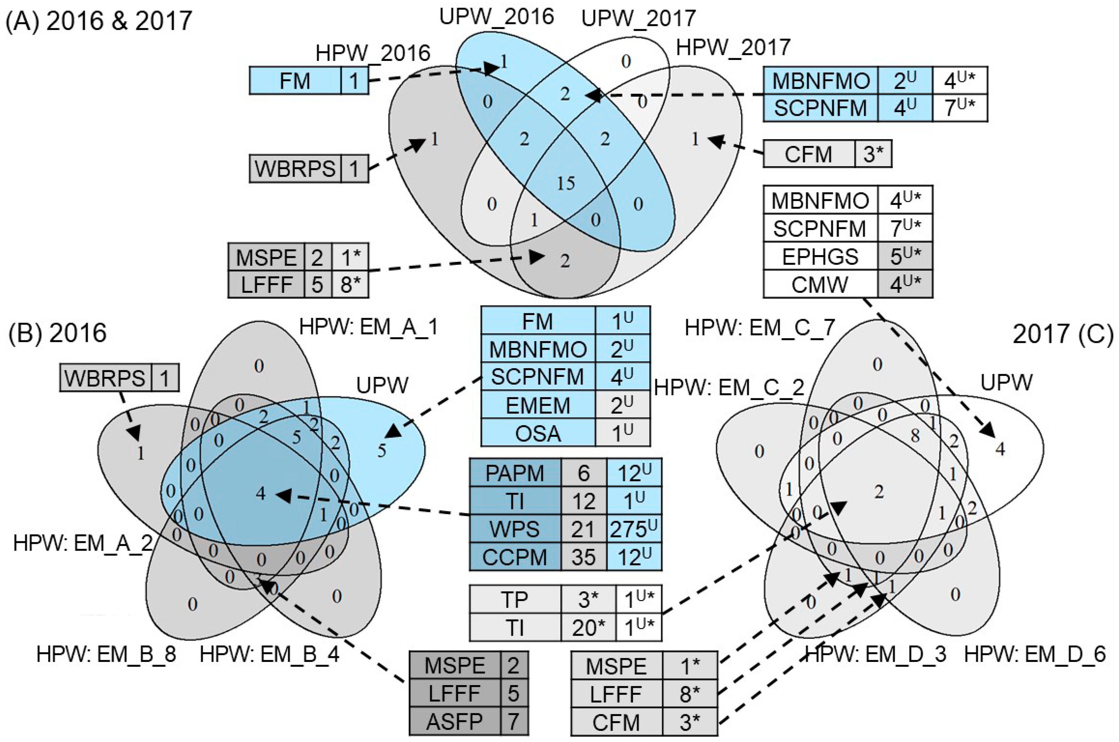
3.2.3. Analyses of Heavily Polluted and Unpolluted Economic Activities in the YRB

All economic activities in the UPW_2017 cluster were in other clusters in the meantime (Figure 5). Industry FM (manufacture of furniture) only appeared in the UPW_2016 cluster with only one JS factory. Industry WBRPS (wood processing and products of wood, bamboo, rattan, palm, and straw) only appeared in HPW_2016 with only one HB factory and industry CFM (manufacture of chemical fibers) only appeared in HPW_2017 with three factories in the provinces of AH and HeN. Industries MBNFMO (mining and beneficiation of non-ferrous metal ores) and SCPNFM (smelting, calendaring, and processing of non-ferrous metals) both appeared in clusters UPW_2016 and UPW_2017. Industries EPHGS (electric power and heat generation and supply) and CMW (coal mining and washing) belonged to the HPW cluster in 2016 and turned into the UPW cluster in 2017, indicating less polluted risk. Industries EMEM (manufacture of electrical machinery and equipment) and OSA (other service activities) belonged to UPW in 2016 and turned into HPW in 2017, indicating more polluted risk.

The industrial classes, namely CCPM (manufacture of chemicals and chemical products, I_26), WPS (water production and supply, I_46), and TI (textile industry, I_17), had the most sewage outlets in the HPW clusters in both 2016 and 2017, and they belonged to divisions 20, 36, 37, and 13 of the ISIC document, respectively (Table S7). The three industrial classes were included in the top 10 industrial classes ranking the numbers of factories in each industry (Figure S1, Table S2). The WPS factories appeared in both the HPW and UPW clusters. The concentration ranges of the pollutants in their wastewater discharges were large (COD: 5.1–215.1 mg L⁻¹; NH₃-N: 0.1–26 mg L⁻¹) and the discharge limits for the factories were different (COD: 30–500 mg L⁻¹; NH₃-N: 1.5–100 mg L⁻¹). The information shows that they were not all municipal wastewater treatment factories but that some were in specific industrial parks. Therefore, the classification should be improved with a thorough consideration of environmental effects, so that it is more accurate and disaggregated and the analytical and policy needs of the sector can be more closely matched [51]. To date, China has mainly concentrated on petrochemical enterprises and sewage outlets in environmentally sensitive areas along the Yangtze River [4]. There are, however, electrical machinery and equipment factories, classified as EMEM, in the SC province that discharge acidic wastewater with pH values between 0.8 and 2.8, with more than 75% of the values over the industrial standard limit in 2017. Some service activities in JS classified as OSA had high average annual COD concentrations in 2017 (92.0 mg L⁻¹, more than 77.6 mg L⁻¹ in 2016) and should be examined to determine how their potential to pollute nearby rivers can be reduced. Overall, the EM clustering makes it possible to explore the whole-basin polluted distribution of wastewater discharges from all economic activities together from an objective perspective in a large river basin.

3.3. Differences in the Pollutants in Wastewater and Economic Activities between the Heavily Polluted and Unpolluted Zones in the YRB

3.3.1. Differences in the Pollutant Concentrations in the Heavily Polluted Wastewater Discharges between the Heavily Polluted and Unpolluted Zones and Analyses of the Economic Activities in the YRB

As shown by the spatial PAM clustering (see Section 3.1), the PAM2 zone with HuN3 was identified as heavily polluted (the HPZ zone) and the HPW sewage outlets (see Section 3.2.2) in PAM2 were identified as possible point sources for the heavily polluted site, HuN3. The PAM3 zone with sites HB2 and HeN1 was identified as unpolluted (the UPZ zone) and the HPW sewage outlets were thought to be related to sites HB2 and HeN1, which were unpolluted. The pollutants in the wastewater discharged in the PAM2 zone were analyzed and compared with the wastewater discharged in PAM3.

Based on the EM clustering in Section 3.2.2, pollutant concentrations in different EM clusters (the HPW and UPW clusters) of the YRB sewage outlets in the HPZ and UPZ for 2016 and 2017 were compared (Figure 6). The EM_A and EM_B classification results for 2016 showed that the HPW in 2016 included 20 sewage outlets with high COD (median of 115.8 mg L⁻¹) and NH₃-N (median of 7.2 mg L⁻¹) (EM_A_1), 4 with abnormal pH values (from 4.25 to 9.76) (EM_A_2), 11 sewage outlets with high COD (174.4 mg L⁻¹) and NH₃-N (8.0 mg L⁻¹) (EM_B_EM8), and 18 with high NH₃-N (8.6 mg L⁻¹) (EM_B_EM4) in the HPZ, while the UPW in 2016 included 6 from EM_A_1 with median COD and NH₃-N values of 87.6 and 8.8 mg L⁻¹, respectively, 3 from EM_A_2 with pH values between 6.95 and 9.98, 6 from EM_B_8 (median COD: 116.5 mg L⁻¹; median NH₃-N: 9.6 mg L⁻¹), and 10 from EM_B_4 (median NH₃-N: 9.4 mg L⁻¹). The HPW in 2017 included 2 sewage outlets with low pH (2.25) (EM_C_2), 11 with high COD (137.3 mg L⁻¹) and NH₃-N (9.9 mg L⁻¹) (EM_C_7), 11 with high COD (median: 100.8 mg L⁻¹) and NH₃-N (median: 10.6 mg L⁻¹) (EM_D_EM3), and 16 with high COD (104.8 mg L⁻¹) (EM_D_6), while the UPW in 2017 included 3 from EM_C_7 (median COD: 43.1 mg L⁻¹, median NH₃-N: 10.8 mg L⁻¹), 11 from EM_D_3 (median COD: 120.2 mg L⁻¹, median NH₃-N: 7.5 mg L⁻¹), and 7 from EM_D_6 (COD: 112.8 mg L⁻¹).

The yearly means of COD and NH₃-N in all the wastewater discharges in the same cluster were different from their medians (

Table 1. Summary data for the weekly means of COD and NH₃-N in the YRB wastewater in the different clusters in 2016 and 2017.

Year	Pollutant	EM_PAM Cluster	Sample Number	Yearly Mean (mg L−1)	Yearly Median (mg L−1)	Welch t-Test P	Wilcoxon Test P	Welch t-Test T	Wilcoxon Test T	Weekly Means
										MAX (mg L−1)		MIN (mg L−1)	SD (mg L−1)	CV
2016	COD	HPW_PAM2	1072	120.7	99.3	(−14.8, 8.4) /	(−5.5, 11.5) /	(−6.2, 6.5)	(−9.4, 1.5)	489.6	0.0		82.6	0.68
		HPW_PAM3	347	123.9	84.6			(−26.5, −2.9)	(−36.5, −18.5)	490.2	4.9		99.4	0.80
		UPW_PAM2	4021	19.4	16.8	(−2.2, 0.8) /	(−3.4, −2.2) *	(2.9, 4.0)	(2.0, 2.9)	324.5	0.0		13.4	0.69
		UPW_PAM3	1235	20.9	20.4			(2.3, 3.6)	(2.3, 3.5)	61.5	0.0		10.0	0.48
	NH3-N	HPW_PAM2	1590	6.9	5.9	(−0.3, 0.6) /	(−0.3, 0.4) /	(−2.0, −0.8)	(−1.4, −0.5)	30.0	0.0		5.9	0.86
		HPW_PAM3	888	6.8	5.1			(−1.4, −0.1)	(−1.4, −0.1)	28.6	0.1		5.8	0.85
		UPW_PAM2	4040	0.5	0.3	(−0.1, −0.0) *	(−0.1, −0.0) *	(−0.0, 0.0)	(0.0, 0.0)	9.2	0.0		0.5	1.13
		UPW_PAM3	1189	0.5	0.4			(−0.0, 0.0)	(−0.0, 0.0)	5.7	0.0		0.5	1.02
2017	COD	HPW_PAM2	1242	120.6	99.8	(−24.7, −11.4) *	(−24.9, −13.1) *	/	/	451.6	1.4		71.9	0.60
		HPW_PAM3	765	138.6	124.2			*	*	486.5	0.0		75.2	0.54
		UPW_PAM2	3426	16.0	14.8	(−2.4, −1.5) *	(−3.0, −2.2) *	*	*	153.6	0.0		9.5	0.60
		UPW_PAM3	2324	17.9	17.6			*	*	73.3	0.0		7.9	0.44
	NH3-N	HPW_PAM2	676	8.3	7.1	(0.1, 1.5) *	(−0.2, 1.0) /	*	*	29.9	0.0		6.8	0.82
		HPW_PAM3	434	7.5	6.8			*	*	29.2	0.0		5.6	0.75
		UPW_PAM2	3410	0.5	0.3	(−0.1, −0.0) *	(−0.1, −0.0) *	/	*	6.8	0.0		0.5	1.14
		UPW_PAM3	2273	0.5	0.4			/	/	6.4	0.0		0.5	0.96

Note: The superscript ^P represents the Welch t−test and Wilcoxon test between clusters PAM2 and PAM3. The superscript ^T represents the Welch t-test and Wilcoxon test between 2016 and 2017, the numbers in parentheses represent the 95% confidence intervals, asterisk (*) represents p < 0.05 and slash (/) represents p > 0.05.

) and the data sets of weekly pollutant concentration means in each cluster were not statistically normally distributed, with unequal sample sizes and nonhomogeneous variances. Application of the Wilcoxon test showed that the yearly medians of COD and NH₃-N were larger in the HPW_PAM2 cluster than in the HPW_PAM3 cluster in 2016, but the difference was not significant. Application of the Welch t-test and the Wilcoxon test showed that the yearly means and medians of NH₃-N were larger in the HPW_PAM2 cluster than in the HPW_PAM3 cluster in 2017, but the differences were not significant. Although the yearly means and medians of COD and NH₃-N were smaller in the UPW_PAM2 cluster than in the UPW_PAM3 cluster in both 2016 and 2017, the maximum weekly means of COD and NH₃-N were all larger in the UPW_PAM2 cluster than in the UPW_PAM3 cluster in both 2016 and 2017 (Table 1 and Figure S4). The yearly means and medians of COD in HPW_PAM3 and NH₃-N in HPW_PAM2 and HPW_PAM3 were significantly larger in 2017 than in 2016, while the yearly means and medians of COD in UPW_PAM2 and UPW_PAM3 were significantly lower in 2017 than in 2016.

Anomaly identification and extreme pollution are important to the water environment management [52,53]. Besides yearly means and medians, the wastewater generation factories with the maximum 2016 and 2017 weekly means of COD and NH₃-N discharges in the PAM2 and PAM3 clusters were also identified. The maximum weekly mean COD in 2016 (489.6 mg L⁻¹) in the HPW_PAM2 cluster belonged to an outlet from a CCPM factory that produced nitrogen fertilizer in the HB province, and in the HPW_PAM3 cluster, a TI factory in the HeN province reached a maximum of 490.2 mg L⁻¹ in 2016, close to the wastewater inlet limit of 500 mg L⁻¹ of the industrial park sewage treatment plant. In 2017, the maximum COD discharging weekly means in the HPW_PAM2 (451.6 mg L⁻¹) and HPW_PAM3 (486.5 mg L⁻¹) clusters were from factories that manufactured starches and starch products belonging to the industry of the processing of agricultural and sideline foods (ASFP) in the HB and AH provinces, respectively. The NH₃-N weekly mean concentration reached a maximum in wastewater discharged from the HB HPW_PAM2 factory (30.0 mg L⁻¹), which produced nitrogen fertilizer and was classified as CCPM, in both 2016 and 2017. Extremely high COD values greater than 500 mg L⁻¹ were recorded in wastewater discharged from the AH HPW_PAM3 factory in December 2017, and were attributed to an instrument failure in the online monitoring system, which was published on the self-monitoring network platform. This discharge was conveyed to the industrial park sewage treatment plant for further treatment (which was also published on the self-monitoring network platform) and so the high concentration does not indicate the true risk and this anomaly needed to be labeled markedly with the real-time data correlation in advance on the network platform. Therefore, the EM clustering results helped to concentrate on the anomalies that happened due to some special reasons, such as monitoring problems, other than actual pollution activities.

Overall, while the COD or NH₃-N concentrations in the wastewater discharged in the HPZ (both in the HPW and UPW clusters) were not significantly higher than those in the UPZ, the wastewater from the sewage outlets in the HPZ tended to be more acidic, and had higher COD and NH₃-N concentrations (the UPW had higher maximum weekly means of pollutants) than that in the UPZ. The data for wastewater discharged in the YRB extended from 2016 to 2017 and the number of sewage outlets with relatively high COD concentrations increased from 2016 to 2017 while those with relatively high NH₃-N concentrations decreased. It is concluded that the simple yearly means and medians of the discharge pollutants from all the factories in a specific cluster may obscure the differences between the clusters and heavily polluted wastewater identification with anomaly detection is necessary so sample numbers and extremums from real-time monitoring data need to be considered thoroughly as evidence for pollution hot spots.

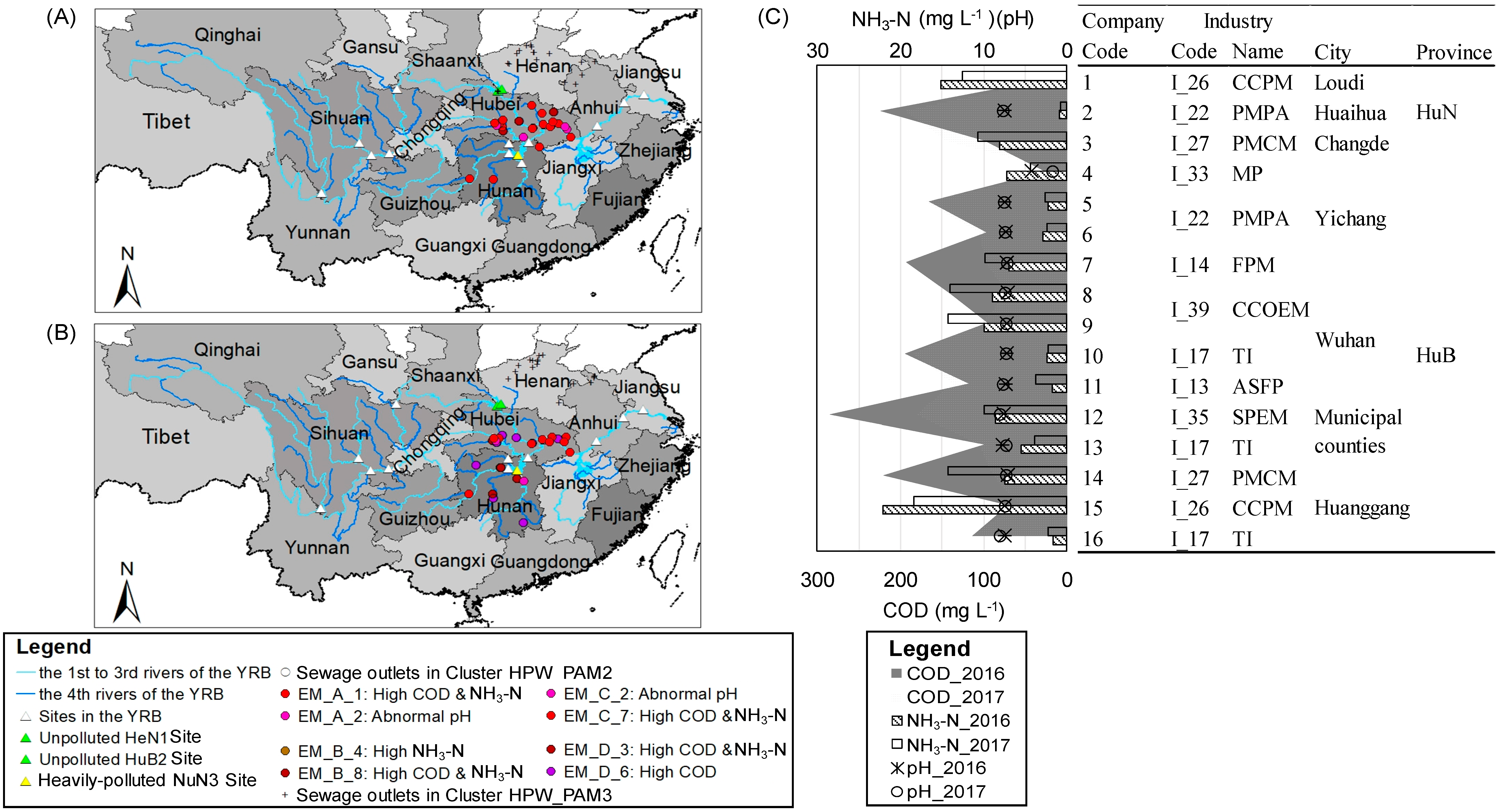
3.3.2. Geographical, Administrative, and Economic Distributions of Heavily Polluted Wastewater Discharges in the Heavily Polluted and Unpolluted Zones in the YRB

Sewage outlets with heavily polluted wastewater discharges (HPW) are marked in Figure 7A,B. In 2016, there were 37 HPW factories in 7 cities in HuN and 10 districts in HB belonging to 14 industrial classes; of these, 12 HPW factories manufactured chemicals and chemical products (CCPM) (Table S8). In 2017, there were 27 factories in 7 cities in HuN and 5 districts in HB belonging to 12 industrial classes, 5 of which were from PMCM (Table S9). The HPW numbers decreased from 26 to 17 in HB and from 11 to 10 in HuN from 2016 to 2017, and it seemed HB had stricter policies on water pollution management than HuN. About 1061 km of the Yangtze’s course runs through central China’s HB province, the most of any province. This province has approved an action plan for reducing pollution and protecting the environment along the Yangtze [4], which may have contributed to the improved water quality in 2017. Xinhua reported that secret pollution discharges were found in several chemical industry parks along the Yangtze in HuN, which indicates that the current law enforcement there is not sufficiently tough [2].

Most PAM3 factories with heavily polluted wastewater (HPW_PAM3) in 2016 and 2017 were not really located in the YRB (Figure 7A,B), according to their geographic positions and details of the factories published online. Two factories in HB that were in the HPW_PAM3 cluster were less than 5 km from HuB2 in the YRB. The concentrations of NH₃-N (9.0–11.2 mg L⁻¹) and/or COD (94.9 mg L⁻¹) in the wastewater discharged from these factories in 2016 were high; for 2017, there was no information about the discharges from one of the factories online, while the COD (60.4 mg L⁻¹) and NH₃-N (5.6 mg L⁻¹) concentrations in the wastewater from the other were not classified in the HPW clusters. Therefore, the risks of pollution from the main point sources to the river in the UPZ were lower in 2017, which shows that to protect the MR-SNWDP drinking water source, wastewater management has improved considerably [48].

There were 16 factories (3 in HuN and 13 in HB) in the HPW_PAM2 cluster in both 2016 and 2017 (Figure 7C). The COD values in the wastewater discharged from their sewage outlets were lower in 2017 than 2016, but the NH₃-N concentrations in the wastewater were similar for both years. Two WPS factories in HB and one WPS factory in HuN were clustered in HPW (cluster EM_B_2) in 2016 and had relatively high annual mean NH₃-N (6.0–11.2 mg L⁻¹) concentrations in their discharge. These factories were not in HPW in 2017 and their discharge had lower NH₃-N values (0.3–6.2 mg L⁻¹). The NH₃-N concentrations in discharges from the two factories in HB exceeded the limit more than 50% of the time in 2016 but only 20% of the time in 2017. Overall, the quality of the wastewater discharged in the HPZ was better in 2017 than in 2016 (http://news.cnhubei.com/). However, the simple yearly means and medians of the discharge pollutants from all the factories in a specific cluster could not show this improvement in wastewater management without the identification of heavilypolluted wastewater discharges in specific factories.

Of the 41 wastewater-generating industrial classes in the YRB, a total of 15 (14 in 2016 and 12 in 2017, Table S7) discharged wastewater with relatively high COD and NH₃-N concentrations, regardless of their discharge limits or discharge standards for each industry [54,55,56,57]. Even from factories in the same industrial class, different wastewater outlets executed different discharge standards with different discharge limits of a specific pollutant. Therefore, no matter whether the standards are exceeded, the discharge concentrations from all economic activities should be considered together. Overall, the PAM spatial clustering and EM water quality clustering were combined to make possible an exploration of the pollution distribution differences in the wastewater discharges from all economic activities together from an objective perspective between the heavily polluted zone with heavily polluted surface water sites and the unpolluted zone with unpolluted surface water sites in a large river basin.

3.4. Temporal Variations in the Pollution Characteristics and Relationships between Heavily Polluted Wastewater Discharges and Surface Water in the Heavily Polluted YRB Zone

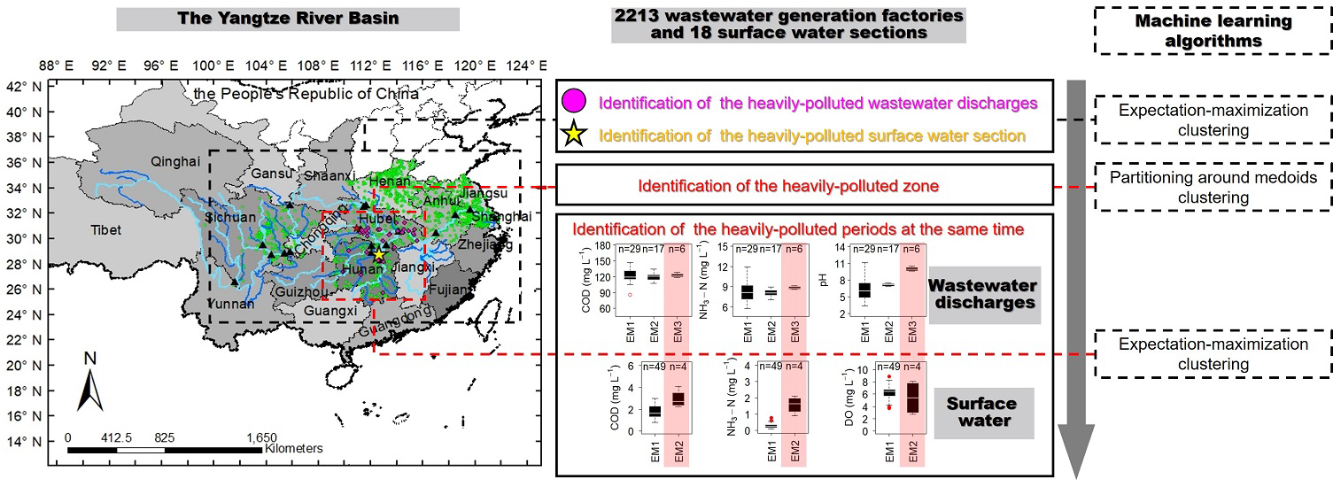
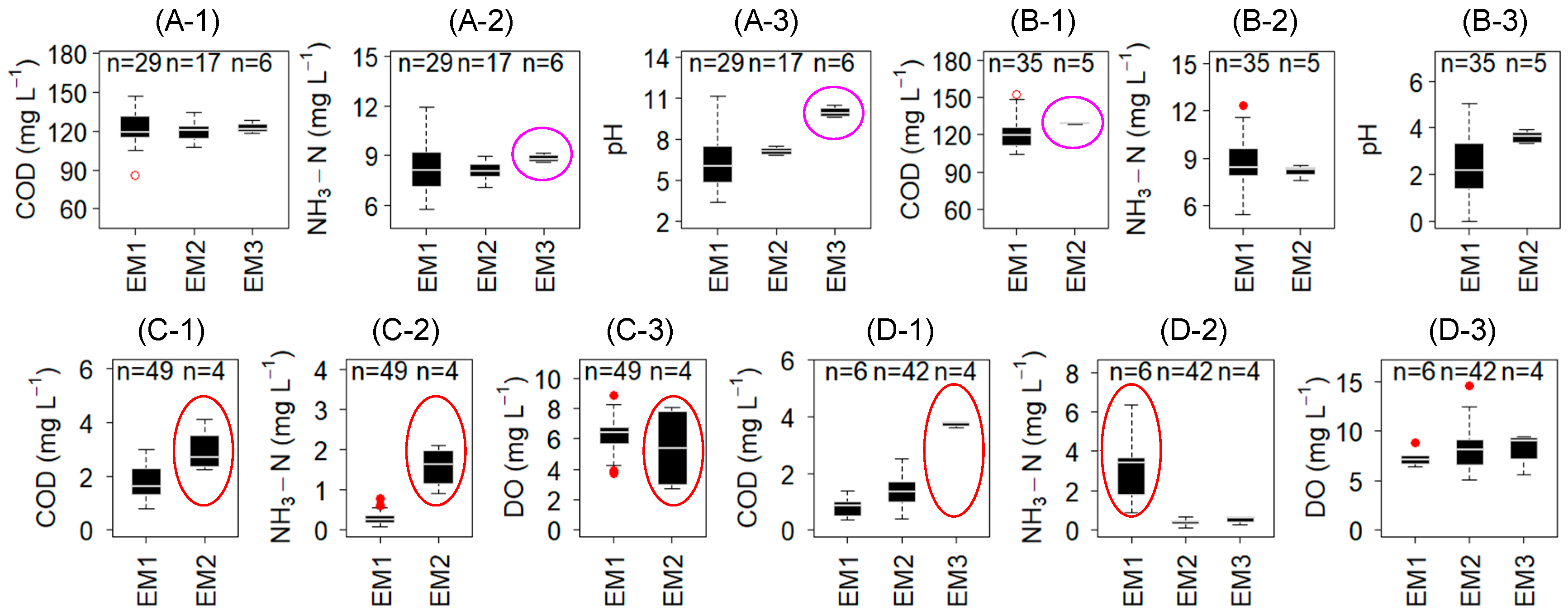
3.4.1. Identification of Heavily Polluted Periods Using EM Clustering Based on Weekly Data for Heavily Polluted Wastewater Discharges and Heavily Polluted Surface Water in the Heavily Polluted YRB Zone

The weekly means of COD, NH₃-N, and pH in wastewater from the HPW_PAM2 sewage outlets in the HPZ were analyzed with the EM clustering method by the Mclust VVI model in 2016 (EM_E) and by Mclust VEI (diagonal, equal shape) model in 2017 (EM_F) (Table S3). The results showed that the weekly medians of NH₃-N (8.74 mg L⁻¹, Welch t-test: p < 0.05, Wilcoxon test: p < 0.05) and pH (9.9, Welch t-test: p < 0.05, Wilcoxon test: p < 0.05) were significantly higher in weeks 15, 18, 19, 20, 22, and 23 (the second quarter) in 2016 in cluster EM3, based on the EM_E method, and the weekly medians of COD (129.6 mg L⁻¹, Welch t-test: p < 0.05, Wilcoxon test: p < 0.05) were significantly higher in weeks 2, 5, 8, 11, and 29 (the first and third quarters) in 2017 in the EM2 cluster, based on the EM_F method (Figure 8A,B), than in the other weeks. The acidic wastewater at the HPW_PAM2 sewage outlets (pH < 6) throughout all of 2017 was mainly from the two outlets in the EM_C_2 cluster (see Section 3.3.1, Figure 6C-5).

The EM clustering results from HuN3 by the Mclust VEI model in 2016 (EM_SC) and by the Mclust EVI (diagonal, equal volume, varying shape) model (EM_SD) (Table S3) showed that the weekly medians of COD (2.68 mg L⁻¹) and NH₃-N (1.62 mg L⁻¹) were relatively high, while those of DO (5.38 mg L⁻¹) were relatively low, in weeks 26, 27, 48, and 49 (June, July, November, and December) in 2016 in the EM2 cluster, based on the EM_SC method, and the weekly medians of COD (3.80 mg L⁻¹) were relatively high in weeks 9, 10, 11, and 27 (February, March, June, and July) in the EM3 cluster and the weekly medians of NH₃-N (3.41 mg L⁻¹) were relatively high in weeks 32, 35, 36, 37, 39, and 48 (August, September, and November) of 2017 in the EM1 cluster, based on the EM_SD method (Figure 8C,D).

The water at HuN3 was polluted and was classified as worse than the national polluted standard limits [11] from weeks 25 to 32 and week 48 (June, July, August, and November) in 2016 and in weeks 35, 36, 37, 39, and 48 (August and September) in 2017 (Figure S3). Overall, the water quality at HuN3 was relatively poor in the second quarter of 2016, when the DO was relatively low, and in the third quarter of 2017, when the NH₃-N was relatively high. Wastewater outlets in the same spatial region were characterized by relatively high NH₃-N concentrations and high pH values in the second quarter of 2016 and high COD concentrations in the third quarter of 2017. The second quarter of 2016 and the third quarter of 2017 could be identified as heavily polluted periods both in surface water and wastewater discharges in the heavily polluted YRB zone. Clusters of weekly water quality in surface water illustrate more details of seasonal pollution variations in rivers [8,47] and clusters of weekly pollutant discharges give more temporal information of point sources to aid decision-making in pollution control and water resource management.

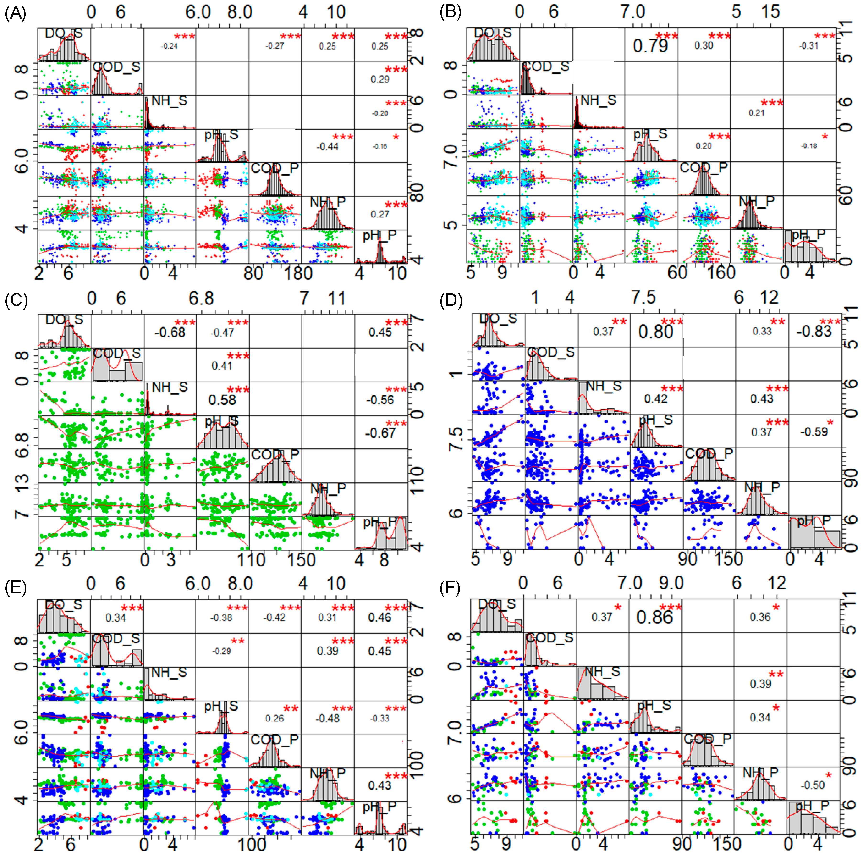
3.4.2. Temporal Correlations between Heavily Polluted Surface Water and Heavily Polluted Wastewater Discharges in the Heavily Polluted YRB Zone

Results from the Spearman correlation analyses (Figure 9, most data did not statistically obey normal distribution by the normal distribution test) showed the temporal correlation of the daily means of COD, NH₃-N, pH, and DO between surface water at the HPS_HuN3 and wastewater discharges in the HPW clusters in the same HPZ. In 2016, the daily mean DO at HuN3 was significantly correlated with COD (−0.27, p < 0.001) in HPW wastewater discharges. The daily mean DO, COD, NH₃-N, and pH at HuN3 were significantly correlated with the pH in the HPW_PAM2 wastewater discharge (DO_S: 0.25, p < 0.001; COD_S: 0.29, p < 0.001; NH _S: −0.20, p < 0.001; pH_S: −0.16, p < 0.05) (Figure 9A). The daily mean NH₃-N in 2017 at HuN3 was significantly and positively correlated with the HPW_PAM2 wastewater (0.21; p < 0.001) (Figure 9B).

The site samples and wastewater discharge samples in the second quarter of 2016 and the third quarter of 2017 with heavily polluted wastewater discharges and surface water (see Section 3.4.1) were also analyzed for temporal correlations (Figure 9C,D). In the second quarter of 2016, the daily mean DO, NH₃-N, and pH values at HuN3 were significantly correlated with the pH in the HPW_PAM2 wastewater discharge (DO_S: 0.45, p < 0.001; p < 0.001; NH _S: −0.56, p < 0.001; pH_S: −0.67, p < 0.001) (Figure 9C). The daily mean NH₃-N in the third quarter of 2017 at HuN3 was significantly and positively correlated with the HPW_PAM2 wastewater (0.43; p < 0.001) (Figure 9D), and the correlation coefficient was larger than 0.21 from the whole year data set. The site samples and wastewater discharge samples in 2016 and 2017 with polluted surface water (monitoring indicators over the national polluted standard limits [11]) were also analyzed for temporal correlations (Figure 9E,F). The samples occurred mainly in the second and third quarters of 2016 and 2017 (marked in green and blue colors). The daily mean DO in the polluted water at HuN3 was significantly correlated with COD (−0.42, p < 0.001) in HPW wastewater discharges in 2016 and the daily mean NH₃-N in the polluted water at HuN3 was significantly correlated with NH₃-N (0.39, p < 0.001) in HPW wastewater discharges in 2017 (Figure 8D). Their correlation coefficient absolute values were larger than 0.27 and 0.21 from the whole year data set, separately.

The DO daily means in the surface water at HuN3 had a stronger significant and negative correlation with the NH₃-N daily means in the surface water in the second quarter of 2016 (−0.68 > −0.27, p < 0.001, Figure 9C) but had a stronger significant and positive correlation with the NH3-N daily means in polluted wastewater discharges (0.31 > 0.25, p < 0.001, Figure 9E) than those from the whole year data sets, and there were no significant correlations between NH3-N in the surface water and in the wastewater discharges. This negative correlation between DO and NH3-N in surface water mainly existed in the samples with low DO concentrations (<5 mg L⁻¹, Figure 9C) and can be explained by the biological activities between dissolved oxygen and reduced ammonia nitrogen in surface water and more sophisticated chemical and biological processes happening from the wastewater discharges (as a source of pollutants) to the surface water (as a sink of pollutants) [58]. In contrast to the 2016 samples with low DO concentrations, in the 2017 data set, the daily mean NH₃-N had significate and positive correlations with the daily mean DO in the surface water in the third quarter and in the polluted periods of 2017 (Figure 9D,F). This is because DO generally had higher concentrations (>5 mg L⁻¹) in 2017 than 2016, indicating a different redox environment, where dissolved oxygen and ammonia had different effect mechanisms on each other with different biological or chemical activities [59]. Moreover, ammonia nitrogen in the wastewater discharges had a higher positive correlation with that in the surface water in 2017 than in 2016 (Figure 9C–F), which should draw the attention to the economic activities with ammonia production.

Overall, correlations between dissolved oxygen/ammonia nitrogen in surface water and organic matters (indicated by COD)/ammonia nitrogen strengthened as the whole-year data sets were reduced to the heavily polluted periods by the EM clustering and water quality evaluation based on weekly data. These temporal correlations show that the bad water quality at HuN3 and the wastewater discharges in the same spatial region were more than coincidental. Management of the pollutants from the point (sewage, sullage, and industrial effluent, etc.) and non-point (urban and rural runoff, etc.) sources are equally important for sustainable management of water resources [8,22,60]. In order to achieve good water quality in rivers, the point sources should be identified and the problematic or ineffective sewage treatment plants should be located and upgraded [61]. More real-time data from wastewater generation factories offers more chances for accurate identification of heavily polluted point sources and heavily polluted periods and unsupervised machine learning techniques, such as clustering algorithms, offer more objective and efficient methods for spatiotemporal pollution identification. The Ministry of Ecology and Environment (known as the State Environmental Protection Administration before September 2018), China’s top environmental watchdog, implemented a three-year action plan in 2018 to clamp down on environmental offenses, including fabrication of and interference with monitoring data [62]. Therefore, the discharge data from the self-monitoring network platform of each company that is published online is available and helpful but needs to be verified further to be more valid if it is to be used to support management.

4. Conclusions

Spatial clustering algorithms, such as the partitioning around medoids (PAM) algorithm, and water quality clustering algorithms, such as the expectation–maximization (EM) algorithm, could be combined as unsupervised machine learning techniques for the identification of heavily polluted wastewater discharges from all economic activities and heavily polluted surface water in a large river basin and for the exploration of their source–sink spatio–temporal relationships to offer more objective and reliable methods to support water resource management.

More than 33% of the industrial classes of wastewater-generating economic activities discharged effluent with high COD and NH₃-N concentrations, regardless of the discharge limits outlined in the discharge standards for pollutants for each industrial class. The results also showed that some wastewater-generating factories in each industry did not follow the discharge standards of their industry and tended to use the highest discharge limits (for COD or NH₃-N) from either older or integrated wastewater discharge standards (see the self-monitoring network platform of each company). In cases where concentrations of pollutants in discharges are above the standards, the high discharge pollutant concentrations in all wastewater-generating industrial classes should be considered together, regardless of the discharge limits or the company-specific standards.

The quality of both the surface water and wastewater discharges was bad in the same spatial region in the YRB in some periods in 2016 and 2017. The fact that the surface water and wastewater discharges were both of low quality at the same time in the same geographical region should be of interest to water resource managers. Also, the spatial and temporal characteristics of pollution should be studied as the GDP grows and economic activities change in the large river basin. The factors that connect the surface water and the wastewater discharges should be studied using data with higher spatial and temporal resolutions and dynamic source–sink synergy mechanisms should be studied further with some prediction models, such as an artificial neural network and support vector machine, in the future [63,64,65].

References

1. UN-Water. The United Nations World Water Development Report, 2017: Wastewater: The Untapped Resource; UNESCO CLD: Paris, France, 2017. [Google Scholar]
2. Xinhua. China Battles Chemical Pollution along Yangtze. Available online: http://english.mep.gov.cn/News_service/media_news/201610/t20161011_365297.shtml (accessed on 30 August 2018).
3. Xinhua. China Releases Yangtze Environmental Protection Plan. Available online: http://english.mep.gov.cn/News_service/media_news/201707/t20170724_418374.shtml (accessed on 30 August 2018).
4. MEP, P.R.C. Cleaner, Greener Yangtze on the Agenda. Available online: http://english.mep.gov.cn/News_service/media_news/201712/t20171229_428830.shtml (accessed on 30 August 2018).
5. Bach, P.M.; Rauch, W.; Mikkelsen, P.S.; McCarthy, D.T.; Deletic, A. A critical review of integrated urban water modelling Urban drainage and beyond. Environ. Mod. Softw. 2014, 54, 88–107. [Google Scholar] [CrossRef]
6. Beck, M.B.; Reda, A. Identification and application of a dynamic-model for operational management of water-quality. Water Sci. Technol. 1994, 30, 31–41. [Google Scholar] [CrossRef]
7. Liu, R.M.; Xu, F.; Zhang, P.P.; Yu, W.W.; Men, C. Identifying non-point source critical source areas based on multi-factors at a basin scale with SWAT. J. Hydrol. 2016, 533, 379–388. [Google Scholar] [CrossRef]
8. Wu, Y.; Chen, J. Investigating the effects of point source and nonpoint source pollution on the water quality of the East River (Dongjiang) in South China. Ecol. Indic. 2013, 32, 294–304. [Google Scholar] [CrossRef]
9. Cortés, U.; Sànchez-Marrè, M.; Ceccaroni, L.; R-Roda, I.; Poch, M. Artificial intelligence and environmental decision support systems. Appl. Intell. 2000, 13, 77–91. [Google Scholar] [CrossRef]
10. Eggimann, S.; Mutzner, L.; Wani, O.; Schneider, M.Y.; Spuhler, D.; de Vitry, M.M.; Beutler, P.; Maurer, M. The Potential of Knowing More: A Review of Data-Driven Urban Water Management. Environ. Sci. Technol. 2017, 51, 2538–2553. [Google Scholar] [CrossRef] [PubMed] [Green Version]
11. Di, Z.; Chang, M.; Guo, P. Water Quality Evaluation of the Yangtze River in China Using Machine Learning Techniques and Data Monitoring on Different Time Scales. Water 2019, 11, 339. [Google Scholar] [CrossRef]
12. Rauch, W.; Urich, C.; Bach, P.M.; Rogers, B.C.; de Haan, F.J.; Brown, R.R.; Mair, M.; McCarthy, D.T.; Kleidorfer, M.; Sitzenfrei, R.; et al. Modelling transitions in urban water systems. Water Res. 2017, 126, 501–514. [Google Scholar] [CrossRef] [PubMed]
13. Romero, J.M.P.; Hallett, S.H.; Jude, S. Leveraging big data tools and technologies: Addressing the challenges of the water quality sector. Sustainability 2017, 9, 19. [Google Scholar] [CrossRef]
14. Chini, C.M.; Stillwell, A.S. The state of us urban water: Data and the energy-water nexus. Water Resour. Res. 2018, 54, 1796–1811. [Google Scholar] [CrossRef]
15. Rui, Y.H.; Fu, D.F.; Minh, H.D.; Radhakrishnan, M.; Zevenbergen, C.; Pathirana, A. Urban Surface Water Quality, Flood Water Quality and Human Health Impacts in Chinese Cities. What Do We Know? Water 2018, 10, 18. [Google Scholar] [CrossRef]
16. Borah, D.K.; Ahmadisharaf, E.; Padmanabhan, G.; Imen, S.; Mohamoud, Y.M. Watershed models for development and implementation of total maximum daily loads. J. Hydrol. Eng. 2019, 24, 18. [Google Scholar] [CrossRef]
17. Meyer, A.M.; Klein, C.; Funfrocken, E.; Kautenburger, R.; Beck, H.P. Real-time monitoring of water quality to identify pollution pathways in small and middle scale rivers. Sci. Total Environ. 2019, 651, 2323–2333. [Google Scholar] [CrossRef] [PubMed]
18. Fan, J.; Han, F.; Liu, H. Challenges of big data analysis. Natl. Sci. Rev. 2014, 1, 293–314. [Google Scholar] [CrossRef] [PubMed]
19. Aghabozorgi, S.; Seyed Shirkhorshidi, A.; Ying Wah, T. Time-series clustering—A decade review. Inform. Syst. 2015, 53, 16–38. [Google Scholar] [CrossRef]
20. Hill, D.J.; Minsker, B.S. Anomaly detection in streaming environmental sensor data: A data-driven modeling approach. Environ. Mod. Softw. 2010, 25, 1014–1022. [Google Scholar] [CrossRef]
21. Mandel, P.; Maurel, M.; Chenu, D. Better understanding of water quality evolution in water distribution networks using data clustering. Water Res. 2015, 87, 69–78. [Google Scholar] [CrossRef]
22. Osmi, S.F.C.; Malek, M.A.; Yusoff, M.; Azman, N.H.; Faizal, W.M. Development of river water quality management using fuzzy techniques: A review. Int. J. River Basin Manag. 2016, 14, 243–254. [Google Scholar] [CrossRef]
23. Zou, H.; Zou, Z.; Wang, X. An Enhanced K-Means Algorithm for Water Quality Analysis of The Haihe River in China. Int. J. Environ. Res. Public Health 2015, 12, 14400–14413. [Google Scholar] [CrossRef]
24. Li, D.; Wang, S.; Li, D. Spatial Data Mining: Theory and Application; Springer: Berlin, Germany, 2015; p. 329. [Google Scholar]
25. Zhang, Q.; Couloigner, I. A new and efficient k-medoid algorithm for spatial clustering. In Proceedings of the Computational Science and Its Applications—ICCSA 2005, Singapore, 9–12 May 2005; Springer: Berlin, Germany, 2015; pp. 181–189. [Google Scholar]
26. Wu, X.; Kumar, V.; Ross Quinlan, J.; Ghosh, J.; Yang, Q.; Motoda, H.; McLachlan, G.J.; Ng, A.; Liu, B.; Yu, P.S.; et al. Top 10 algorithms in data mining. Knowl. Inf. Syst. 2008, 14, 1–37. [Google Scholar] [CrossRef]
27. Brunton, S.L.; Kutz, J.N. Data-Driven Science and Engineering: Machine Learning, Dynamical Systems, and Control; Cambridge University Press: Cambridge, UK, 2019. [Google Scholar]
28. Dempster, A.P.; Laird, N.M.; Rubin, D.B. Maximum likelihood from incomplete data via the EM algorithm. J. R. Stat. Soc. B Ser. B Meth. 1977, 39, 1–22. [Google Scholar] [CrossRef]
29. Do, C.B.; Batzoglou, S. What is the expectation maximization algorithm? Nat. Biotechnol. 2008, 26, 897. [Google Scholar] [CrossRef] [PubMed]
30. Adler, J. R in a Nutshell: A Desktop Quick Reference; O’Reilly Media, Inc.: Sebastopol, CA, USA, 2010. [Google Scholar]
31. Omar, S.; Ngadi, A.; Jebur, H.H. Machine learning techniques for anomaly detection: An overview. Int. J. Comput. Appl. 2013, 79. [Google Scholar] [CrossRef]
32. Editorial Committee of Encyclopedia of rivers and lakes in China. In Section of Changjiang River Basin; China Water & Power press: Beijing, China, 2010; Volume 1, p. 510.
33. Wikipedia. Yangtze. Available online: https://en.wikipedia.org/wiki/Yangtze (accessed on 30 August 2018).
34. General Office MEP. Ministry of Environmental Protection, the People’s Republic of China, Beijing, China, 2015. Available online: http://www.mee.gov.cn/gkml/hbb/bgt/201602/t20160204_329897.htm (accessed on 2 September 2018).
35. GAQSIQ, P.R.C.; SA, P.R.C. Industrial Classification for National Economic Activities, Vol. GB/T 4754-2017; General Administration of Quality Supervision, Inspection and Quarantine and Standardization Administration, the People’s Republic of China: Beijing, China, 2017; p. 222.
36. UN-DESA-SD. Series M No. 4/Rev.4, Department of Economic and Social Affairs, Statistics Division, 2008. Available online: https://unstats.un.org/unsd/publication/seriesm/seriesm_4rev4e.pdf (accessed on 30 August 2018).
37. General Office MEP; Ministry of Environmental Protection. 2016 Report on the State of the Environment in China; Ministry of Environmental Protection: Beijing, China, 2016.
38. Wang, X.P.; Zhang, F.; Kung, H.T.; Ghulam, A.; Trumbo, A.L.; Yang, J.Y.; Ren, Y.; Jing, Y.Q. Evaluation and estimation of surface water quality in an arid region based on EEM-PARAFAC and 3D fluorescence spectral index: A case study of the Ebinur Lake Watershed, China. Catena 2017, 155, 62–74. [Google Scholar] [CrossRef]
39. China National Environmental Monitoring Centre. Weekly Reports on National Surface Water Quality Automatic Monitoring; China National Environmental Monitoring Centre: Beijing, China, 2016; Available online: http://www.cnemc.cn/sssj/szzdjczb/ (accessed on 1 February 2018).
40. China National Environmental Monitoring Centre. Real-Time Data on National Surface Water Quality Automatic Monitoring Publishing System; China National Environmental Monitoring Centre: Beijing, China, 2016; Available online: http://58.68.130.147/# (accessed on 1 February 2018).
41. Zhao, Y. R and Data Mining: Examples and Case Studies; Academic Press: Cambridge, MA, USA, 2012. [Google Scholar]
42. Schubert, E.; Rousseeuw, P.J. Faster k-Medoids Clustering: Improving the PAM, CLARA, and CLARANS Algorithms. arXiv 2018, arXiv:1810.05691. [Google Scholar]
43. Hennig, C.; Liao, T.F. How to find an appropriate clustering for mixed-type variables with application to socio-economic stratification. J. R. Stat. Soc. Ser. C (Appl. Stat.) 2013, 62, 309–369. [Google Scholar] [CrossRef] [Green Version]
44. Scrucca, L.; Fop, M.; Murphy, T.B.; Raftery, A.E. mclust 5: Clustering, classification and density estimation using gaussian finite mixture models. R J. 2016, 8, 289. [Google Scholar] [CrossRef] [PubMed]
45. Hollander, M.; Wolfe, D.A.; Chicken, E. Nonparametric Statistical Methods, 3rd ed.; John Wiley & Sons: Hoboken, NJ, USA, 2015; p. 751. [Google Scholar]
46. Cortez, B.; Carrera, B.; Kim, Y.-J.; Jung, J.-Y. An architecture for emergency event prediction using LSTM recurrent neural networks. Expert Syst. Appl. 2018, 97, 315–324. [Google Scholar] [CrossRef]
47. Chen, P.; Li, L.; Zhang, H.B. Spatio-Temporal Variations and Source Apportionment of Water Pollution in Danjiangkou Reservoir Basin, Central China. Water 2015, 7, 2591–2611. [Google Scholar] [CrossRef] [Green Version]
48. People’s Daily & China.org.cn. Biggest Water Transfer Project Ever Benefits 100 mln in China. Available online: http://english.mee.gov.cn/News_service/media_news/201706/t20170622_416491.shtml (accessed on 1 September 2018).
49. Wilson, M.; Li, X.-Y.; Ma, Y.-J.; Smith, A.; Wu, J. A review of the economic, social, and environmental impacts of China’s South–North Water Transfer Project: A sustainability perspective. Sustainability 2017, 9, 1489. [Google Scholar] [CrossRef]
50. World Health Organization. 2018. Available online: https://www.who.int/water_sanitation_health/monitoring/coverage/wastewater-country-files/en/ (accessed on 18 January 2019).
51. UN-Water GLAAS. Trackfin Initiative: Tracking Financing to Sanitation, Hygiene and Drinking-Water at National Level: Guidance Document; World Health Organization: Geneva, Switzerland, 2017. [Google Scholar]
52. Deng, W.H.; Wang, G.Y. A novel water quality data analysis framework based on time-series data mining. J. Environ. Manag. 2017, 196, 365–375. [Google Scholar] [CrossRef] [PubMed]
53. Hou, D.B.; Liu, S.; Zhang, J.; Chen, F.; Huang, P.J.; Zhang, G.X. Online Monitoring of Water-Quality Anomaly in Water Distribution Systems Based on Probabilistic Principal Component Analysis by UV-Vis Absorption Spectroscopy. J. Spectrosc. 2014, 2014, 150636. [Google Scholar] [CrossRef]
54. MEP, P.R.C.; GAQSIQ, P.R.C. Discharge Standard of Water Pollutants for Ammonia Industry, Vol. GB 13458-2013; Ministry of Environmental Protection and General Administration of Quality Supervision, Inspection and Quarantine: Beijing, China, 2013; p. 8.
55. MEP, P.R.C.; GAQSIQ, P.R.C. Discharge standards of water pollutants for dyeing and finishing of textile industry, Vol. GB 4287-2012; Ministry of Environmental Protection and General Administration of Quality Supervision, Inspection and Quarantine: Beijing, China, 2012; p. 9.
56. MEP, P.R.C.; GAQSIQ, P.R.C. GAQSIQ, P.R.C. Discharge Standard of Water Pollutants for Starch Industry, Vol. GB25461-2010; Ministry of Environmental Protection and General Administration of Quality Supervision, Inspection and Quarantine: Beijing, China, 2010; p. 10.
57. MEP, P.R.C.; GAQSIQ, P.R.C. Discharge Standard of Pollutants for Municipal Wastewater Treatment Plant, Vol. GB 18918-2002; State Environmental Protection Administration and General Administration of Quality Supervision, Inspection and Quarantine: Beijing, China, 2003; p. 12.
58. Cun, C.; Vilagines, R. Time series analysis on chlorides, nitrates, ammonium and dissolved oxygen concentrations in the Seine river near Paris. Sci. Total Environ. 1997, 208, 59–69. [Google Scholar] [CrossRef]
59. EPA, U.S. Aquatic Life Ambient Water Quality Criteria for Ammonia—Freshwater 2013; Office of Water, U.S. EPA: Washington, DC, USA, 2013. Available online: https://www.epa.gov/sites/production/files/2015-08/documents/aquatic-life-ambient-water-quality-criteria-for-ammonia-freshwater-2013.pdf (accessed on 15 May 2018).
60. Zhou, P.; Huang, J.; Pontius, R.G.; Hong, H. New insight into the correlations between land use and water quality in a coastal watershed of China: Does point source pollution weaken it? Sci. Total Environ. 2016, 543, 591–600. [Google Scholar] [CrossRef] [PubMed]
61. Al-Mamun, A.; Zainuddin, Z.J.I.E.J. Sustainable river water quality management in Malaysia. IIUM Eng. J. 2013, 14. [Google Scholar] [CrossRef]
62. Ministry of Environmental Protection. The 2018 National Working Conference on Environmental Protection Held in Beijing. Available online: http://english.mep.gov.cn/About_MEE/leaders_of_mee/liganjie/Activities_lgj/201802/t20180213_431467.shtml (accessed on 30 August 2018).
63. Alizadeh, M.J.; Kavianpour, M.R.; Danesh, M.; Adolf, J.; Shamshirband, S.; Chau, K.-W. Effect of river flow on the quality of estuarine and coastal waters using machine learning models. Eng. Appl. Comput. Fluid Mech. 2018, 12, 810–823. [Google Scholar] [CrossRef] [Green Version]
64. Olyaie, E.; Banejad, H.; Chau, K.-W.; Melesse, A.M. A comparison of various artificial intelligence approaches performance for estimating suspended sediment load of river systems: A case study in United States. J. Environ. Monit. Manag. 2015, 187, 189. [Google Scholar] [CrossRef] [PubMed]
65. Shamshirband, S.; Jafari Nodoushan, E.; Adolf, J.E.; Abdul Manaf, A.; Mosavi, A.; Chau, K.-W. Ensemble models with uncertainty analysis for multi-day ahead forecasting of chlorophyll a concentration in coastal waters. Eng. Appl. Comput. Fluid Mech. 2019, 13, 91–101. [Google Scholar] [CrossRef]
Figure 1. The 18 surface water sites that were part of the national monitoring program and the 2386 sewage outlets from the 2213 factories that were part of the national monitoring network in the 7 administrative regions (ARs) in the Yangtze River Basin YRB (YRB) in 2016 and 2017.
Water 11 01268 g001
Figure 2. Spatial partitioning around medoids (PAM) clustering of the 18 surface water sites and the 2213 wastewater-generating factories (also their 2386 monitored sewage outlets) in the Yangtze River Basin in 2016 and 2017.
Water 11 01268 g002
Figure 3. Classification of the 18 YRB surface water sites in 2016 (A,B) and 2017 (C,D) by expectation–maximization (EM) clustering based on the yearly means (Y_means) of chemical oxygen demand (COD), ammonia nitrogen (NH3-N), pH, and DO. Data distribution (A,C) and geographical distribution (B,D). (The different shapes and colors in Figure 3A,C and diamonds, x crosses, crosses, triangles, and circles in Figure 3B,D indicate different EM clusters.).
Water 11 01268 g003
Figure 4. Data distribution vs. classifications of the YRB sewage outlets using EM clustering and the yearly means of COD, NH3-N, and pH in wastewater discharged in 2016 (A: the EM_A method and B: the EM_B method) and 2017 (C: the EM_C method and D: the EM_D method) (different shapes and colors indicate different EM clusters).
Water 11 01268 g004
Figure 5. Economic activities and numbers of heavily polluted and unpolluted YRB wastewater-generating factory clusters calculated with different clustering algorithms in 2016 (A) and 2017 (B) (In figures, the acronyms represent the cluster names and the numbers represent the number of industrial classes in each cluster. In tables, the acronyms represent the industrial class names and the numbers represent the number of factories in each industry in each cluster. The superscript U represents the number of factories in the UPW (unpolluted wastewater) clusters and the superscript * represents the number of factories in the 2017 clusters).
Water 11 01268 g005
Figure 6. Yearly mean concentrations of COD, NH3-N, and pH vs. EM classifications of the YRB sewage outlets in the HPZ (heavily polluted zone) (sewage outlets in the PAM2 cluster by the PAM clustering: A-1, A-2, A-5, B-1, B-2, C-1, C-2, C-5, D-1, and D-2) and the UPZ (unpolluted zone) (sewage outlets in the PAM3 cluster by the PAM clustering: A-3, A-4, A-6, B-3, B-4, C-3, C-4, C-6, D-3, and D-4) using the EM clustering from 2016 and 2017. (A and B: the classifications of sewage outlets using the EM_A and EM_B methods in Table S3 for 2016; C and D: the classifications of sewage outlets using the EM_C and EM_D methods in Table S3 for 2017; n represents the number of wastewater outlets.).
Water 11 01268 g006
Figure 7. Geographical distribution of sewage outlets with heavily polluted wastewater discharges in the HPZ (heavily polluted zone) with heavily polluted surface water sites and in the UPZ (unpolluted zone) with unpolluted surface water sites in the YRB in 2016 (A) and in 2017 (B) and the yearly means of COD, NH3-N, and pH in the heavily polluted wastewater discharged from the same YRB factories in the HPZ in 2016 and 2017 and their industrial classes and administrative regions (C).
Water 11 01268 g007
Figure 8. EM clustering classifications of discharge weeks of the YRB heavily polluted sewage outlets in the HPZ (heavily polluted zone) based on the weekly means of COD, NH3-N, and pH in wastewater in 2016 (A1–3, EM_E method) and 2017 (B1–3, EM_F method) and EM clustering classifications of monitoring weeks at the HuN3 site (one of the heavily polluted surface water sections in HuN province) based on the weekly means of COD, NH3-N, and DO in surface water in 2016 (C1–3, EM_SC method) and 2017 (D1–3, EM_SD method) (a lowercase n in Figure 8A2–4 and Figure 8B2–4 represents the number of weekly samples in a specific cluster. The weeks heavily polluted by wastewater discharges are marked by pink ovals and the weeks heavily polluted by surface water are marked by red ovals.).
Water 11 01268 g008
Figure 9. Spearman correlation analyses between each pair of daily means of COD, NH3-N, pH, and DO in surface water at HuN3 and in the HPW wastewater discharges in the HPZ zone in 2016. (A: daily samples in the whole year; C: daily samples in the second quarter; E: daily samples with polluted water at HuN3) and 2017 (B: daily samples in the whole year; D: daily samples in the second quarter; F: daily samples with polluted water at HuN3). (DO_S, COD_S, NH_S, and pH_S represent DO, COD, NH3-H, and pH in surface water at HuN3. COD_P, NH_P, and pH_P represent COD, NH3-H, and pH in the HPW discharge wastewater. In the rectangle, figures below the diagonal: points represent daily samples; the point colors represent different quarters of the year: red (the 1st quarter), green (the 2nd quarter), blue (the 3rd quarter), and cyan (the 4th quarter); the red curves represent the fitted curve. In the rectangle, figures above the diagonal: the numbers represent Spearman correlation coefficients between each two variables; the font sizes represent the coefficient value sizes; * represents p < 0.05; ** represents p < 0.01; *** represents p < 0.001. The diagonal figures with gray rectangles represent frequency distribution histograms of each variable.).
Water 11 01268 g009