Contribution of Biological Effects to the Carbon Sources/Sinks and the Trophic Status of the Ecosystem in the Changjiang (Yangtze) River Estuary Plume in Summer as Indicated by Net Ecosystem Production Variations

Abstract
:1. Introduction
2. Materials and Methods
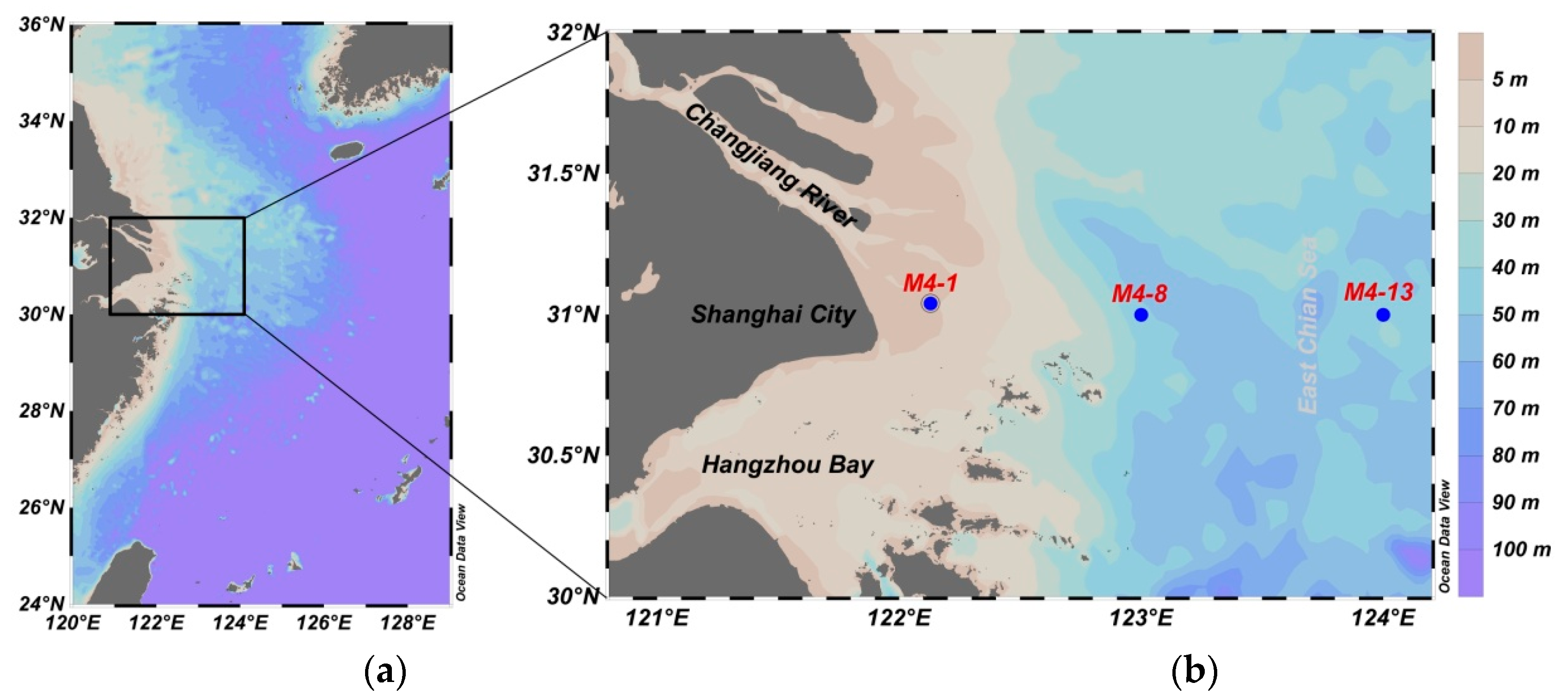
2.1. Study Area
2.2. Sampling Collection
2.3. Hydrographic Measurements
2.4. Mass Balance Model Based on Separating pCO2-Controlling Processes
2.5. Error Analysis
3. Results
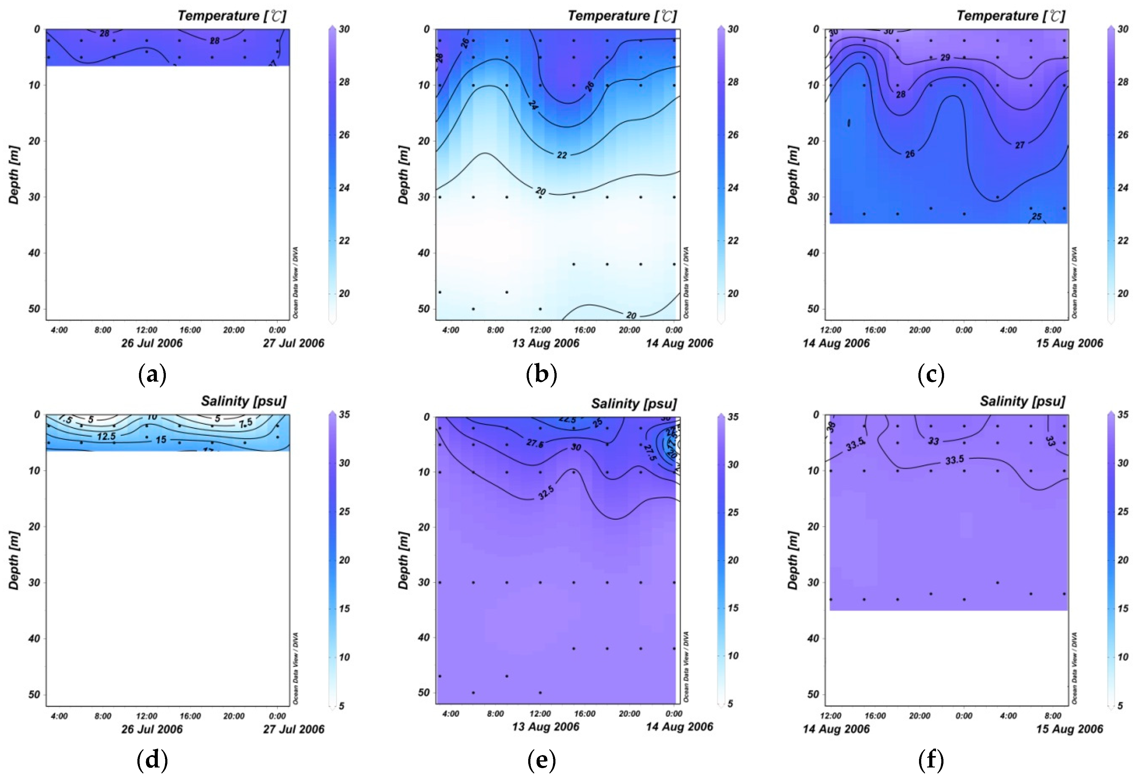
3.1. 24 Hourly Variations in Temperature and Salinity
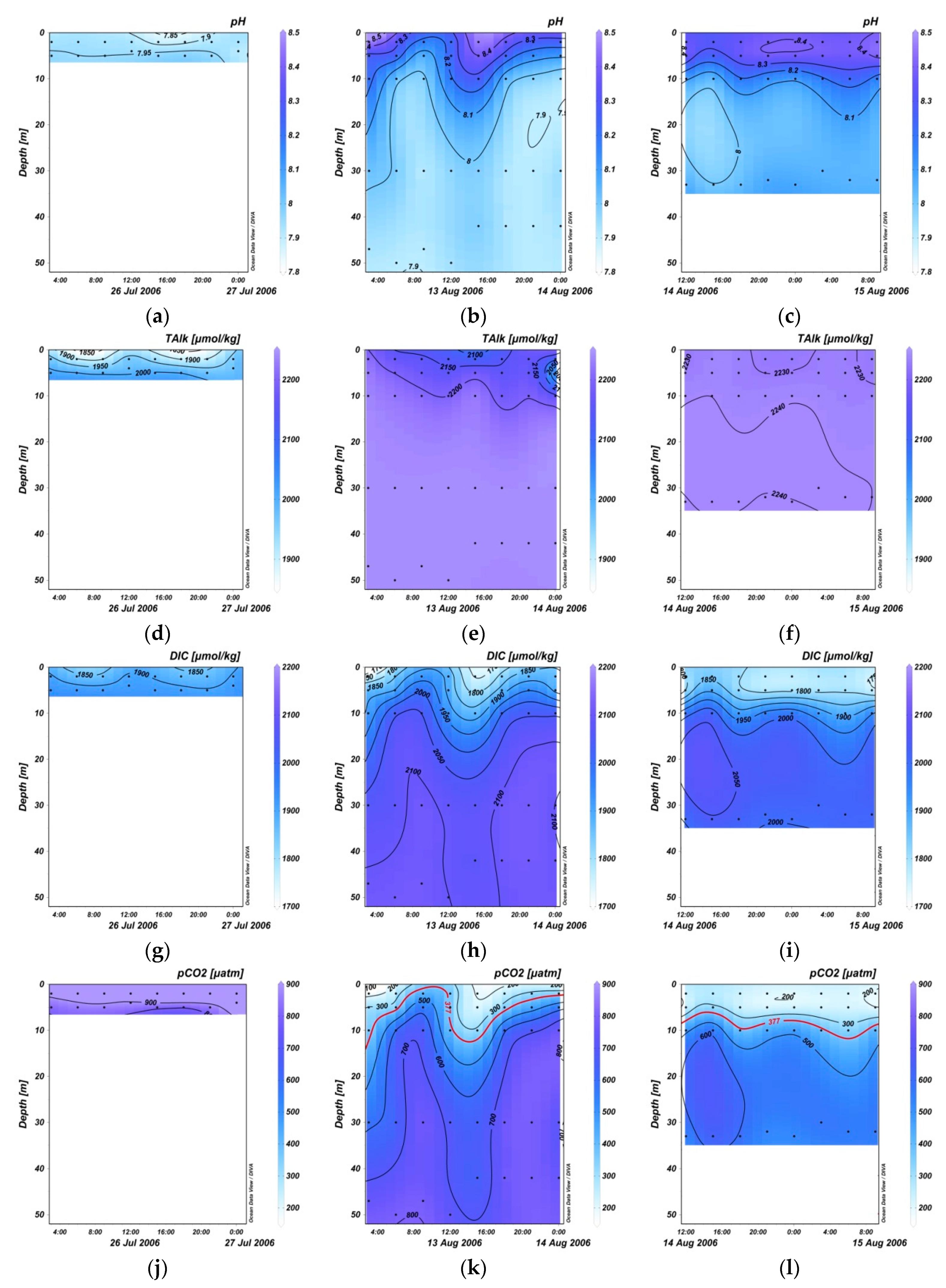
3.2. Variation in pH, TA, DIC, and Sea Surface pCO2 within 24 Hours
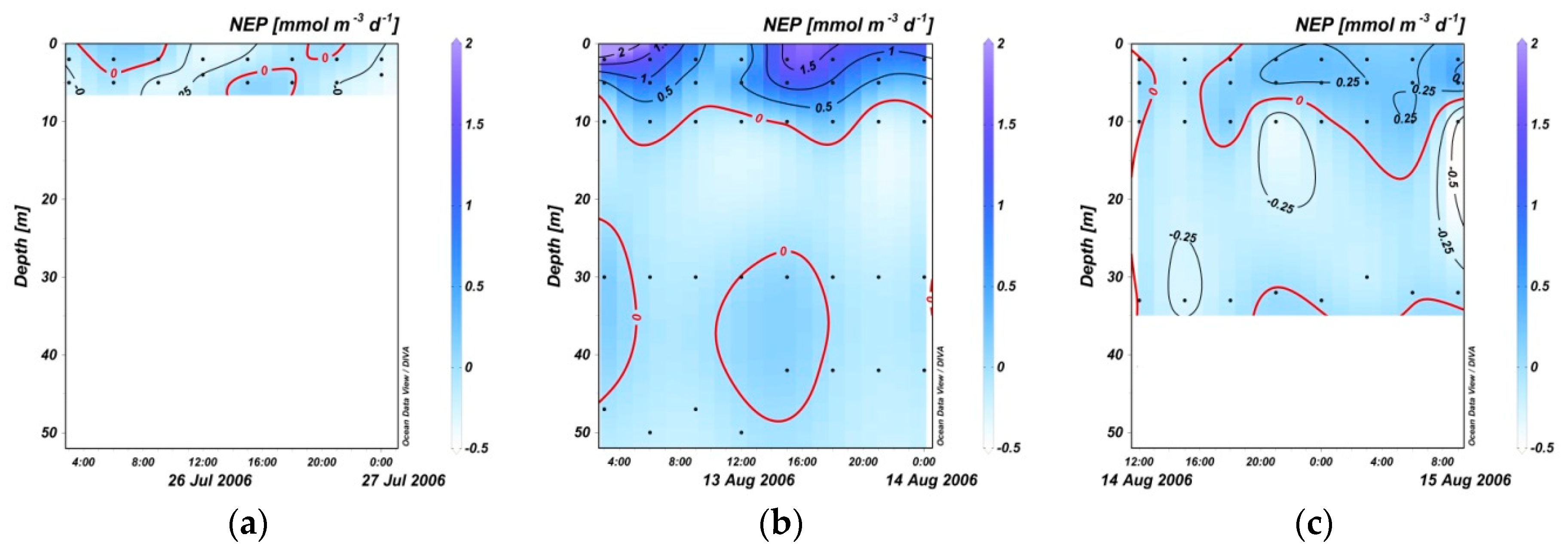
3.3. Variation in NEP within 24 Hours
4. Discussion
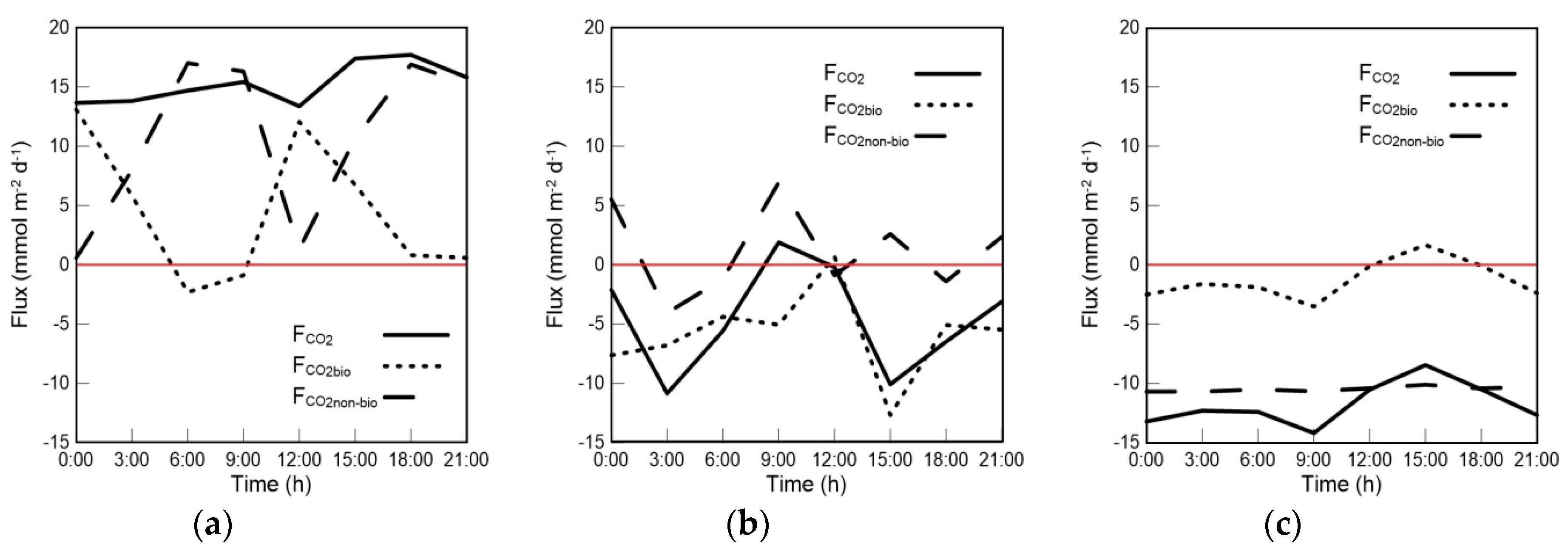
4.1. Variations in FCO2bio and FCO2 in the Mixed Layer
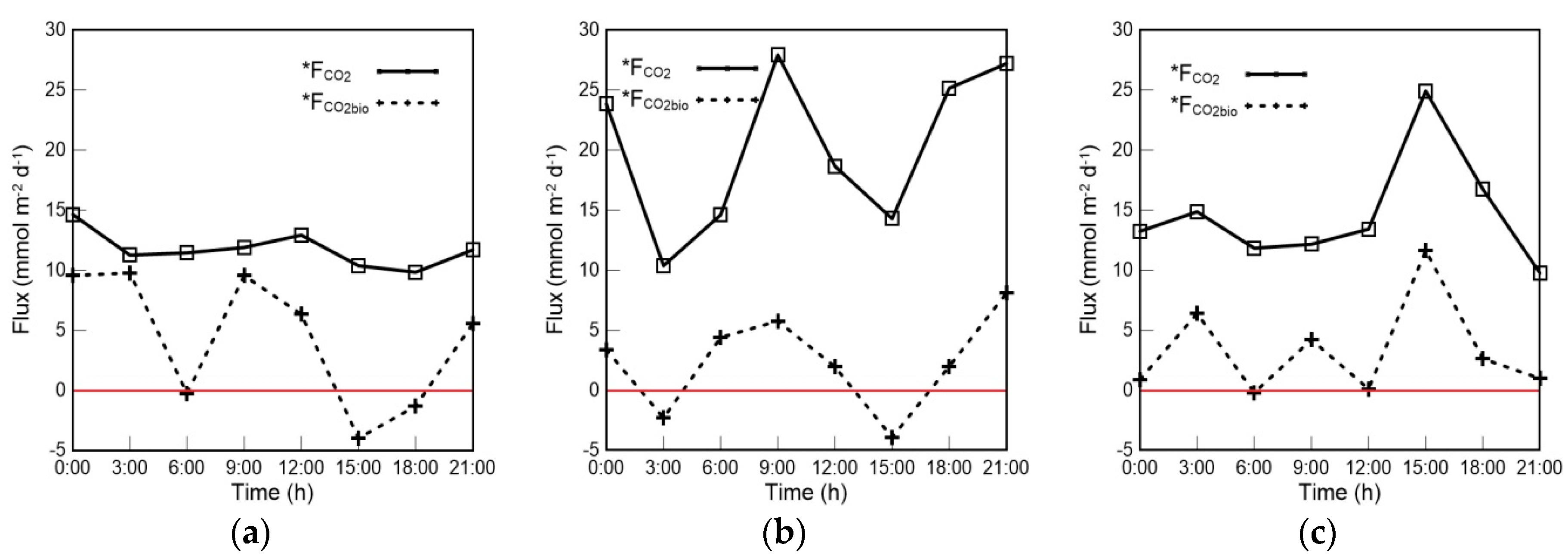
4.2. The Contribution of Biological Processes to the Air–Sea CO2 Exchange Flux in the Mixed Layer
4.3. Potential Carbon Sources under the Mixed Layer
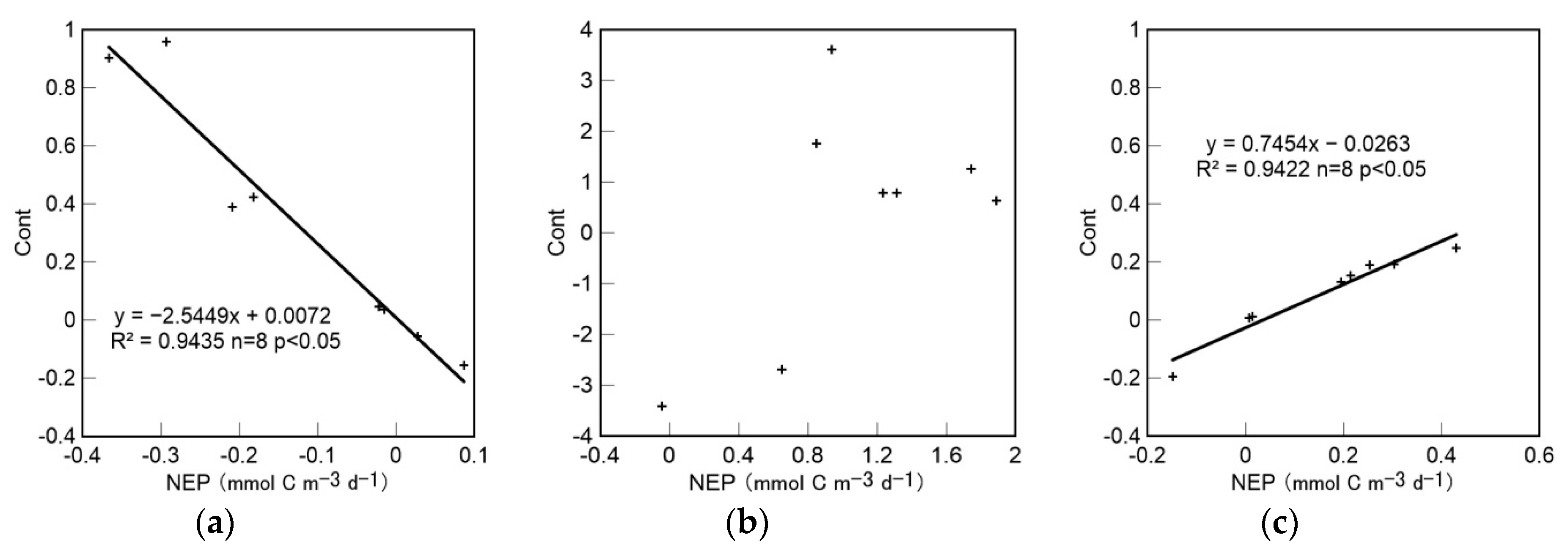
4.4. Trophic Status Assessments and the Relationship between Cont and NEP
5. Conclusions
Author Contributions
Funding
Acknowledgments
Conflicts of Interest
References
- Guo, X.; Zhai, W.; Dai, M.; Zhang, C.; Bai, Y.; Xu, Y.; Li, Q.; Wang, G. Air–Sea CO2 fluxes in the East China Sea based on multiple-year underway observations. Biogeosciences 2015, 12, 5123–5167. [Google Scholar] [CrossRef]
- Song, J.; Qu, B.; Li, X.; Yuan, H.; Li, N.; Duan, L. Carbon sinks/sources in the Yellow and East China Seas—Air-sea interface exchange, dissolution in seawater, and burial in sediments. Sci. China Earth Sci. 2018, 61, 1583. [Google Scholar] [CrossRef]
- Jiao, N.; Liang, Y.; Zhang, Y.; Liu, J.; Zhang, Y.; Zhang, R.; Zhao, M.; Dai, M.; Gao, K.; Song, J.; et al. Carbon pools and fluxes in the China Seas and adjacent oceans. Sci. China Earth Sci. 2018, 61, 1535. [Google Scholar] [CrossRef]
- Chen, C.; Chiang, K.; Gong, G.; Shiah, F.; Tseng, C.; Liu, K. Importance of planktonic community respiration on the carbon balance of the East China Sea in summer. Glob. Biogeochem. Cycles 2006, 20. [Google Scholar] [CrossRef]
- Chen, C.A. The Kuroshio intermediate water is the major source of nutrients on the East China Sea continental shelf. Oceanol. Acta 1996, 19, 523–527. [Google Scholar]
- Wang, K.; Chen, J.; Jin, H.; Gao, S.; Xu, J.; Lu, Y.; Haung, D.; Hao, Q.; Weng, H. Summer nutrient dynamics and biological carbon uptake rate in the Changjiang River plume inferred using a three end-member mixing model. Cont. Shelf Res. 2014, 91, 192–200. [Google Scholar] [CrossRef]
- Li, D.; Chen, J.; Ni, X.; Wang, K.; Zeng, D.; Wang, B.; Jin, H.; Haung, D.; Cai, W. Effects of biological production and vertical mixing on sea surface pCO2 variations in the Changjiang River plume during early autumn: A buoy-based time series study. J. Geophys. Res. Ocean. 2018, 123, 6156–6173. [Google Scholar] [CrossRef]
- Odum, H.T. Primary production in flowing waters. Limnol. Oceanogr. 1956, 1, 102–117. [Google Scholar] [CrossRef]
- Oviatt, C.A.; Doering, P.H.; Nowicki, B.L.; Zoppini, A. Net system production in coastal waters as a function of eutrophication, seasonality and benthic macrofaunal abundance. Estuaries 1993, 16, 247–254. [Google Scholar] [CrossRef]
- Carvalho, M.C.; Schulz, K.G.; Eyre, B.D. Respiration of new and old carbon in the surface ocean: Implications for estimates of global oceanic gross primary productivity. Glob. Biogeochem. Cycles 2017, 31, 975–984. [Google Scholar] [CrossRef]
- Li, X.; Yu, Z.; Song, X.; Cao, X.; Yuan, Y. Nitrogen and phosphorus budgets of the Changjiang River estuary. Chin. J. Oceanol. Limnol. 2011, 29, 762–774. [Google Scholar] [CrossRef]
- Xu, H.; Wolanski, E.; Chen, Z. Suspended particulate matter affects the nutrient budget of turbid estuaries: Modification of the LOICZ model and application to the Yangtze Estuary. Estuar. Coast. Shelf Sci. 2013, 127, 59–62. [Google Scholar] [CrossRef]
- Swaney, D.P.; Howarth, R.W.; Butler, T.J. A novel approach for estimating ecosystem production and respiration in estuaries: Application to the oligohaline and mesohaline Hudson River. Limnol. Oceanogr. 1999, 44, 1509–1521. [Google Scholar] [CrossRef] [Green Version]
- Palevsky, H.I.; Quay, P.D. Influence of biological carbon export on ocean carbon uptake over the annual cycle across the North Pacific Ocean. Glob. Biogeochem. Cycles 2017, 31, 81–95. [Google Scholar] [CrossRef] [Green Version]
- Borges, A.; Schiettecatte, L.-S.; Abril, G.; Delille, B.; Gazeau, F. Carbon dioxide in European coastal waters. Estuar. Coast. Shelf Sci. 2006, 70, 375–387. [Google Scholar] [CrossRef]
- Xuan, J.; Huang, D.; Zhou, F.; Zhu, X.; Fan, X.; Ni, X.; Xing, C. Application of data assimilation to synoptic temperature mapping of the coastal ocean survey. Oceanol. Limnol. Sin. 2012, 43, 17–26. [Google Scholar]
- Dai, A.; Trenberth, K.E. Estimates of freshwater discharge from continents: Latitudinal and seasonal variations. J. Hydrometeorol. 2002, 3, 660–687. [Google Scholar] [CrossRef]
- Liu, X.C. Concentration variation and flux estimation of dissolved inorganic nutrient from the Changjianag River into its estuary. Oceanol. Limnol. Sin. 2002, 32, 332–340. [Google Scholar]
- Wang, K.; Chen, J.; Ni, X.; Zeng, D.; Li, D.; Jin, H.; Glibert, P.; Qiu, W.; Haung, D. Real-time monitoring of nutrients in the Changjiang Estuary reveals short-term nutrient-algal bloom dynamics. J. Geophys. Res. Ocean. 2017, 122, 5390–5403. [Google Scholar] [CrossRef]
- Liu, Q.; Guo, X.; Yin, Z.; Zhou, K.; Roberts, E.; Dai, M. Carbon fluxes in the China Seas: An overview and perspective. Sci. China 2018, 61, 1564–1582. [Google Scholar] [CrossRef]
- Chen, C.; Shiah, F.; Chiang, K.; Gong, G.; Kemp, W. Effects of the Changjiang (Yangtze) River discharge on planktonic community respiration in the East China Sea. J. Geophys. Res. Ocean. 2009, 114. [Google Scholar] [CrossRef] [Green Version]
- Huang, H.; Wang, Y.; Zhang, W. Characteristics of tidal waves in the eastern Jiangsu coast and Changjiang Estuary. In Proceedings of the 2015 International Forum on Energy, Environment Science and Materials, Shenzhen, China, 25–26 September 2015. [Google Scholar]
- Chen, C.A.; Zhai, W.; Dai, M. Riverine input and air-sea CO2 exchanges near the Changjiang (Yangtze River) Estuary: Status quo and implication on possible future changes in metabolic status. Cont. Shelf Res. 2008, 28, 1476–1482. [Google Scholar] [CrossRef]
- Zhejiang Meteorological Bureau. Zhejiang Provincial Climate Bulletin; Zhejiang Meteorological Bureau: Zhejiang, China, 2006.
- Zhai, W.; Dai, M. On the seasonal variation of air-sea CO2 fluxes in the outer Changjiang (Yangtze River) Estuary, East China Sea. Mar. Chem. 2009, 117, 2–10. [Google Scholar] [CrossRef]
- Gao, X.; Song, J.; Li, X.; Li, N.; Yuan, H. pCO2 and carbon fluxes across sea-air interface in the Changjiang Estuary and Hangzhou Bay. Chin. J. Oceanol. Limnol. 2008, 26, 289–295. [Google Scholar] [CrossRef]
- Chou, W.; Gong, G.; Sheu, D.D.; Jan, S.; Huang, C.; Chen, C. Reconciling the paradox that the heterotrophic waters of the East China Sea shelf act as a significant CO2 sink during the summertime: Evidence and implications. Geophys. Res. Lett. 2009, 36, 139–156. [Google Scholar] [CrossRef]
- Lewis, E.; Wallace, D.; Allison, L.J. Program Developed for CO2 System Calculations; Carbon Dioxide Information Analysis Center, managed by Lockheed Martin Energy Research Corporation for the US Department of Energy Tennessee: Nashville, TN, USA, 1998.
- Wang, B.; Chen, J.; Jin, H.; Li, H.; Liu, X.; Zhuang, Y.; Xu, Y.; Zhang, H. Preliminary study on the dissolved inorganic carbon system and its response mechanism in Changjiang River Estuary and its adjacent sea areas in summer. J. Mar. Sci. 2011, 29, 63–70. [Google Scholar]
- Zhai, W.; Chen, J.; Jin, H.; Li, H.; Liu, J.; He, X.; Bai, Y. Spring carbonate chemistry dynamics of surface waters in the northern East China Sea: Water mixing, biological uptake of CO2, and chemical buffering capacity. J. Geophys. Res. Ocean. 2015, 119, 5638–5653. [Google Scholar] [CrossRef]
- Liss, P.S.; Slater, P.G. Flux of gases across the air-sea interface. Nature 1974, 247, 181–184. [Google Scholar] [CrossRef]
- Weiss, R.F. Carbon dioxide in water and seawater: The solubility of a non-ideal gas. Mar. Chem. 1974, 2, 203–215. [Google Scholar] [CrossRef]
- Wanninkhof, R. Relationship between wind speed and gas exchange over the ocean. J. Geophys. Res. 1992, 97, 7373–7382. [Google Scholar] [CrossRef]
- Sweeney, C.; Gloor, E.; Jacobson, A.R.; Key, R.; Mckinley, G.; Sarmiento, J.; Wanninkhof, R. Constraining global air-sea gas exchange for CO2 with recent bomb 14C measurements. Glob. Biogeochem. Cycles 2007, 21. [Google Scholar] [CrossRef]
- Chaturvedi, M.K.M.; Langote, S.D.; Kumar, D.; Asolekar, S. Significance and estimation of oxygen mass transfer coefficient in simulated waste stabilization pond. Ecol. Eng. 2014, 73, 331–334. [Google Scholar] [CrossRef]
- Nixon, S.W. Physical energy inputs and the comparative ecology of lake and marine ecosystems: Physical energy inputs. Limnol. Oceanogr. 1988, 33, 1005–1025. [Google Scholar] [CrossRef]
- Xue, L.; Cai, W.; Hu, X.; Sabine, C.; Jones, S.; Sutton, A.; Jiang, L.; Reimer, J. Sea surface carbon dioxide at the Georgia time series site (2006–2007): Air–sea flux and controlling processes. Prog. Oceanogr. 2016, 140, 14–26. [Google Scholar] [CrossRef]
- Takahashi, T.; Olafsson, J.; Goddard, J.G.; Chipman, D.; Sutherland, S. Seasonal variation of CO2 and nutrients in the high-latitude surface oceans: A comparative study. Glob. Biogeochem. Cycles 1993, 7, 843–878. [Google Scholar] [CrossRef]
- Dickson, A.G.; Millero, F.J. A comparison of the equilibrium constants for the dissociation of carbonic acid in seawater media. Deep Sea Res. Part A Oceanogr. Res. Pap. 1987, 34, 1733–1743. [Google Scholar] [CrossRef]
- Sprintall, J.; Tomczak, M. Evidence of the barrier layer in the surface layer of the tropics. J. Geophys. Res. Ocean. 1992, 97, 7305–7316. [Google Scholar] [CrossRef] [Green Version]
- Mehrbach, C.; Culberson, C.H.; Hawley, J.E.; Pytkowicx, R.M. Measurement of the apparent dissociation constants of carbonic acid in seawater at atmospheric pressure. Limnol. Oceanogr. 1973, 18, 897–907. [Google Scholar] [CrossRef]
- Taylor, J.R. An Introduction to Error Analysis; University Science Books: Sausalito, CA, USA, 1997. [Google Scholar]
- Qu, B.; Song, J.; Li, X.; Yuan, H.; Li, N.; Ma, Q. pCO2 distribution and CO2 flux on the inner continental shelf of the East China Sea during summer 2011. Chin. J. Oceanol. Limnol. 2013, 31, 1088–1097. [Google Scholar] [CrossRef]
- Chen, X.; Song, J.; Yuan, H.; Li, X.; Li, N.; Duan, L.; Qu, B. Preliminary study on the change of carbon exchange at sea-air interface and its regional carbon sink intensity in the summer of 2012 in the East China Sea. Haiyang Xuebao 2014, 36, 18–31. [Google Scholar]
- Zhou, F.; Xuan, J.; Ni, X.; Huang, D. Preliminary Analysis of Dynamic Factors of Summer Yangtze River Freshwater Change between 1999 and 2006. Haiyang Xuebao 2009, 31, 1–12. [Google Scholar]
- Milliman, J.D.; Shen, H.; Yang, Z.; Mead, R. Transport and deposition of river sediment in the Changjiang estuary and adjacent continental shelf. Cont. Shelf Res. 1985, 4, 37–45. [Google Scholar] [CrossRef]
- Zhang, J.; Wu, Y.; Jennerjahn, T.C.; Ittekkot, V.; He, Q. Distribution of organic matter in the Changjiang (Yangtze River) Estuary and their stable carbon and nitrogen isotopic ratios: Implications for source discrimination and sedimentary dynamics. Mar. Chem. 2007, 106, 111–126. [Google Scholar] [CrossRef]
- Borges, A.V.; Delille, B.; Frankignoulle, M. Budgeting sinks and sources of CO2 in the coastal ocean: Diversity of ecosystems counts. Geophys. Res. Lett. 2005, 32, 301–320. [Google Scholar] [CrossRef]
- Cai, W.; Dai, M.; Wang, Y. Air-sea exchange of carbon dioxide in ocean margins: A province-based synthesis. Geophys. Res. Lett. 2006, 33. [Google Scholar] [CrossRef] [Green Version]
- Li, M.; Rong, Z. Effects of tides on freshwater and volume transports in the Changjiang River plume. J. Geophys. Res. Ocean. 2012, 117. [Google Scholar] [CrossRef] [Green Version]


| Sampling Date | Sampling Area | Correlation | Reference |
|---|---|---|---|
| 27 August 2013 | 31–31.5° N, 121.5–124° E (with a salinity of 5.17–34.26) | TA = 13.3507S + 1797.39 | [7] |
| August 2009 | 31° N, 122.5–125° E (Transect C) | TA = 13.2S + 1744.7 | [29] |
| 8–27 April and 2–7 May 2007 | 30.0–31.8° N, 122.5–123.5° E (with a salinity of 13.00–34.49) | TA = 13.5875S + 1823.1 | [30] |
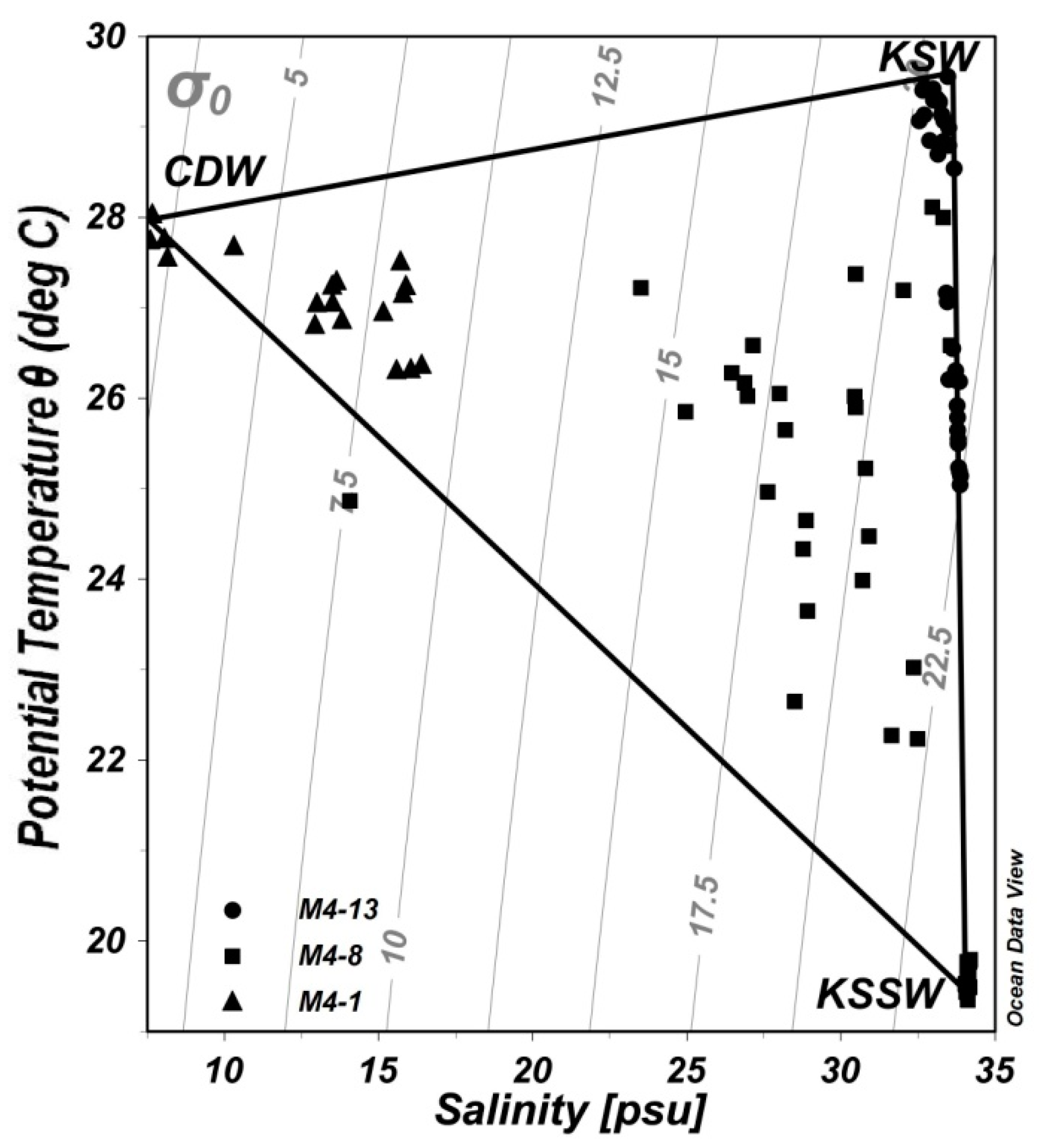
| Sampling Date | θ (°C) | S | TA (μmol kg−1) | DIC (μmol kg−1) |
|---|---|---|---|---|
| CDW | 27.76 ± 0.20 | 7.88 ± 0.28 | 1898 ± 3.6 | 1863 ± 3.6 |
| KSW | 29.49 ± 0.10 | 33.22 ± 0.33 | 2232 ± 4.4 | 1808 ± 0.6 |
| KSSW | 19.48 ± 0.09 | 34.11 ± 0.05 | 2244 ± 0.6 | 2105 ± 13 |
| Regions | Depth | Minimum | Maximum | Mean | Standard Deviation |
|---|---|---|---|---|---|
| Near-shore | Surface | −0.36 | 0.09 | −0.12 | 0.16 |
| Bottom | −0.34 | 0.13 | −0.17 | 0.18 | |
| Front | Surface | −0.04 | 1.89 | 1.07 | 0.62 |
| 5 m | 0.19 | 1.26 | 0.65 | 0.38 | |
| 10 m | −0.32 | 0.28 | −0.05 | 0.20 | |
| 30 m | −0.15 | 0.21 | −0.01 | 0.12 | |
| Bottom | −0.16 | 0.11 | −0.08 | 0.09 | |
| Offshore | Surface | −0.14 | 0.43 | 0.16 | 0.19 |
| 5 m | −0.08 | 0.52 | 0.22 | 0.17 | |
| 10 m | −0.54 | 0.28 | −0.08 | 0.31 | |
| Bottom | −0.31 | 0.03 | −0.09 | 0.12 |
| Regions | 00:00 | 03:00 | 06:00 | 09:00 | 12:00 | 15:00 | 18:00 | 21:00 |
|---|---|---|---|---|---|---|---|---|
| Near-shore | 2.73 | 2.14 | 2.06 | 2.06 | 2.72 | 2.09 | 2.06 | 2.09 |
| Front | 8.49 | 2.94 | 2.18 | 2.36 | 2.83 | 2.07 | 5.11 | 2.35 |
| Offshore | 3.29 | 6.03 | 8.84 | 5.03 | 3.05 | 2.45 | 6.67 | 3.44 |
| Regions | 00:00 | 03:00 | 06:00 | 09:00 | 12:00 | 15:00 | 18:00 | 21:00 | Mean |
|---|---|---|---|---|---|---|---|---|---|
| Near-shore | 96% | 42% | −16% | −6% | 90% | 39% | 5% | 4% | 32% |
| Front | 360% | 63% | 79% | −269% | −341% | 126% | 78% | 175% | 34% |
| Offshore | 19% | 13% | 15% | 25% | 1% | −20% | 1% | 19% | 9% |
© 2019 by the authors. Licensee MDPI, Basel, Switzerland. This article is an open access article distributed under the terms and conditions of the Creative Commons Attribution (CC BY) license (http://creativecommons.org/licenses/by/4.0/).
Share and Cite
Zhang, Y.; Li, D.; Wang, K.; Xue, B. Contribution of Biological Effects to the Carbon Sources/Sinks and the Trophic Status of the Ecosystem in the Changjiang (Yangtze) River Estuary Plume in Summer as Indicated by Net Ecosystem Production Variations. Water 2019, 11, 1264. https://doi.org/10.3390/w11061264
Zhang Y, Li D, Wang K, Xue B. Contribution of Biological Effects to the Carbon Sources/Sinks and the Trophic Status of the Ecosystem in the Changjiang (Yangtze) River Estuary Plume in Summer as Indicated by Net Ecosystem Production Variations. Water. 2019; 11(6):1264. https://doi.org/10.3390/w11061264
Chicago/Turabian StyleZhang, Yifan, Dewang Li, Kui Wang, and Bin Xue. 2019. "Contribution of Biological Effects to the Carbon Sources/Sinks and the Trophic Status of the Ecosystem in the Changjiang (Yangtze) River Estuary Plume in Summer as Indicated by Net Ecosystem Production Variations" Water 11, no. 6: 1264. https://doi.org/10.3390/w11061264