Managing Municipal Wastewater Treatment to Control Nitrous Oxide Emissions from Tidal Rivers


1
Department of Civil Engineering, Indian Institute of Technology Madras, Chennai 600 036, India
2
Department of Civil Engineering, and Coordinator, Indo-German Center for Sustainability, Indian Institute of Technology Madras, Chennai 600 036, India
*
Author to whom correspondence should be addressed.
Water 2019, 11(6), 1255; https://doi.org/10.3390/w11061255
Submission received: 29 April 2019
/
Revised: 1 June 2019
/
Accepted: 9 June 2019
/
Published: 15 June 2019
(This article belongs to the Section Water Quality and Contamination)
Abstract
:Waste load allocation management models were developed for controlling nitrous oxide emissions from a tidal river. The decision variables were treatment levels at wastewater discharging stations and the rate of upstream water release. The simulation model for N2O emissions from the river was embedded in the optimization model and the problem was solved using the simulated annealing technique. In two of the models, the total cost was minimized, while in the third model, emissions from the river were minimized for a specified constraint on the available money. Proof-of-concept studies, with hypothetical scenarios for contaminant loading but realistic flow conditions corresponding to the Tyne River, UK, were carried out. It was found that the treatment cost could be reduced by 36% by treating wastewater discharges in the upper reaches more during the high tide as compared to during low tide. For the same level of N2O emissions, approximately 16.7% lesser costs could be achieved by not only treating the wastewater but also inducing dilution by releasing more water from the upstream side. It was also found that beyond a limit, N2O emissions cannot be reduced significantly by spending more money on treatment and water release.
1. Introduction
Nitrous oxide is one of the most significant greenhouse gases (GHG), with a 10% share of total net anthropogenic radiative forcing with a Global Warming Potential (GWP) ~300 [1]. As human intervention impacts the biogeochemical cycle of nitrogen [2], an increased nitrogen mobilisation, and thus microbial nitrous oxide production, has been observed at an annual rate of 0.25% [3]. Sources of N2O emissions include combustion of fossil fuels, paddy fields, ruminants, coal mines, natural gas transport, fertilisers, and decomposition of organic matter along with waste disposal facilities, etc. [4,5]. In developing countries, high emissions from domestic wastewater disposal can be attributed to the disparity in the development of wastewater treatment infrastructure with population growth [6].
Municipal wastewater, with a sizable fraction of domestic wastewater, is known to contain significant amounts of dissolved organic and inorganic nitrogen and discharge of such wastewater into rivers without treatment may result in significant N2O emission [7]. Vertical velocity variations and DO (dissolved oxygen) consumption by various sources may induce different oxygenated conditions in rivers and estuaries. These conditions favour ammonium oxidation (aerobic) and reduction of nitrate, NO3− (anoxic), which result in N2O emission. Based on laboratory batch and column studies, it was found that N2O generation is caused by nitrification and denitrification processes. Some studies suggested nitrification to be a predominant source of N2O [8,9]. Many past studies have shown rivers and estuaries to be major GHG sources [10,11,12,13,14,15]. Nitrous oxide from estuaries and rivers are predicted to increase by a factor of 3 and 4 respectively by 2050, with rivers becoming the principal contributor as per a global model by Kroeze and Seitzinger [16]. River, estuaries and coastal zones contribute to about 25% of total anthropogenic sources and 10% of total global emissions [17]. In Brisbane estuary, N2O dominated GHG emissions in terms of CO2 equivalents (64%) with water-air flux of 0.1–3.4 mg N2O m−2 d−1 [18]. Field studies by Hu et al. [19] indicated that sewage draining into rivers of Tianjin city, China contributed to high N2O emissions, which are about 1.13–3.12 times compared to those in the natural rivers.
Control of N2O emissions from rivers and estuaries may be possible by complete removal of the nitrogen in wastewater received by various domestic sewage treatment plants (STPs). However, this results in a significant increase in the cost of the wastewater treatment and STP operation. Thus, it becomes important to develop management models for the management of the STP–River system, which can be used for determining optimal operation strategies. Several process-oriented simulation models have been developed in the past for estimating N2O emissions from water columns without consideration of hydrodynamics [20,21]. Many models in the past simulated river water quality in terms of BOD (biological oxygen demand), DO, etc. [22,23,24]. However, only a few hydro-dynamic models have simultaneously considered the reactive transport and emission of N2O from rivers and estuaries. Regnier et al. [25] were probably the first to develop a fully transient one-dimensional reactive transport model, CONTRASTE, which can simulate transport and emission of N2O along with DIN (dissolved inorganic nitrogen) components, DO, suspended matter, pH, salinity, dissolved organic matter, CO2, etc. Rodrigues et al. [26] used a similar one-dimensional hydro-dynamic model for simulating N2O emissions from tidal rivers receiving treated wastewater and applied it to the River Tyne, UK. Garnier et al. [27] developed a model for nitrogen transformations in the lower Seine river and estuary (France) based on the rain-discharge model, RIVERSTRAHLER and microbial reaction kinetics for nitrification and denitrification.
Earlier studies on management models for waste load allocation in rivers focused mostly on the maintenance of minimum DO concentration for river health [28,29,30,31,32,33,34,35,36]. Objective functions in these models are based on minimisation of cost, maximisation in the equitable sharing of treatment burden, maximisation of performance, minimisation of a violation index. Minimisation of the magnitude of violation along with cost minimisation was used in few studies. However, to the authors’ knowledge, no waste load allocation model has been presented to date for control of GHG emissions from rivers receiving partially treated domestic wastewater.
In this work, single objective optimisation models are proposed for optimal waste load allocation in tidal rivers receiving domestic wastewater at different locations. Two different optimisation models are presented. In the first model, the objective function is the minimisation of the total cost of wastewater treatment before its release, while not exceeding a specified level of nitrous oxide emission from the river. In the second model, the objective function is the minimisation of nitrous oxide emission, subject to budgetary constraints. These models consider not only the effect of treatment of wastewater, but also the effect of water releases from an upstream environmental reservoir on the N2O emissions from the river. In both the models, the decision vector comprises of treatment levels at different discharge locations and upstream releases. These waste load allocation models use a water quality simulation model, which numerically solves the complete dynamic equations for water flow, and reactive transport model for N2O [26]. The optimisation problem is solved using the well-established simulated annealing technique.
2. Materials and Methods
Two non-seasonal, deterministic, single objective waste load allocation planning models were formulated in this study. These waste load allocation models embed a water quality simulator using a simulation-optimisation framework. The simulation model determines spatial and temporal variation in N2O emission from a tidal river, for specified (i) water release from upstream, (ii) downstream tidal level variation, (iii) channel characteristics, and (iv) treatment levels at the discharge points of partially treated domestic wastewater.
2.1. Water Quality Simulation Model
The water quality simulation model comprises of two modules: (i) The Flow model and (ii) Reactive transport model.
2.1.1. The Flow Model
The Flow model numerically solves the one-dimensional Saint-Venant equations for flow in a channel [37]. It may be noted that the proposed model is not applicable for flow in an estuary. The governing equations for a non-prismatic rectangular tidal river are:
where, h = flow depth (m), u = cross-sectional averaged flow velocity (m/s), B = width of the river (m), R = hydraulic mean depth = A/P (m), A = Cross sectional area (m2), P = wetted perimeter (m), η = tidal height above a reference datum (m), QL = lateral flow into the river through the loading point, n = Manning’s roughness coefficient of the river bed and g = acceleration due to gravity.
Equations (1) and (2) were numerically solved using the classical Preissmann implicit scheme [37], for the specified initial and boundary conditions. Temporal variation of water release rate, Qu was specified as the upstream boundary condition. Temporal variation in the tidal water level above a mean value was specified as the downstream boundary condition. Tidal level variation was taken as a combination of six harmonic components. To start with, upstream flow rate and the downstream water level corresponded to the lowest level of a large spring tide. Water levels and flow rates at intermediate locations were specified arbitrarily as equal to the boundary values. The flow model was then run for one complete spring-neap cycle (approximately 34 days) to obtain the initial conditions corresponding to the next cycle. Other inputs to the flow model included the cross-sectional characteristics, bed profile, roughness coefficient and lateral inflow values at sewage treatment plant (STP) outlets along the river. Spatial and temporal variations of flow depth in terms of water elevation above mean level and flow rate were obtained as part of the solution.
2.1.2. Transport Model
The reactive transport model in the present study is based on the simple model proposed by Rodrigues et al. [26] for N2O emissions from a tidal river. It simultaneously solves the fate and transport equations for (i) NH4+, (ii) NO3− and (iii) N2O. These equations are based on the following assumptions: (i) All the components are well mixed in the cross-section, and so the transport is considered only in the flow direction. (ii) There is no reduction of N2O into molecular nitrogen, N2. (iii) Generation of NH4+is from a diffuse homogeneous source from sediment at the bed, at the same rate throughout the length of the river. (iv) Although anoxic denitrification in the bed sediment also contributes to N2O generation, it is insignificant and neglected. (v) Nitrous oxide generation is from nitrification in the water column. (vi) Nitrification and algal uptake are first order reactions. It is assumed that most of the organic matter in the wastewater gets treated before nitrogen removal stage and so BOD/COD (chemical oxygen demand) are not tracked in this study.
In the present work, the model developed by Rodrigues et al. [26] has been adopted for simulating the N2O production from the river. This model has been applied to Tyne river in the UK by them. Nitrifiers are usually present in the river, as well as STP effluent. Field data from the Tyne river in the year 2000 [26] indicated that Tyne river was supersaturated with N2O. Much of the nitrification was occurring in the top layers of water column, where the nitrifiers were available from the sewage treatment plant effluent. Although nitrifiers were also present in the river, they were mostly present in the bed sediment. It was hypothesized that these nitrifiers might not be responsible for N2O generation because the suspended sediment concentration in the river was low.
Sediment-generated N2O resulting from the anoxic denitrification may also result in elevated concentrations. However, for the particular case of Tyne river, it was found that the concentration of N2O was much higher near surface waters making the sewage-input NH4 and its nitrification to be the main N2O contributor [26]. It was also found that dissolved oxygen was high along the river [26], making the N2O generation due to anoxic conditions negligible. However, there is a potential for N2O generation due to denitrification in the bed sediment in other rivers.
As the data related to the quantification of bacteria/their growth was not available during their study, Rodrigues et al. [26] have adopted a potential approach for nitrification kinetics. In this approach, bacterial density was parameterised by a single coefficient for nitrification . N2O was an intermediate product of the nitrification process. This model was calibrated for Tyne river. Authors have adopted the same model in the present work. The governing equations may be written as given below [26]:
where, , ; concentrations (mg/L); = longitudinal dispersion coefficient (m2/s); = rate of lateral flow into the river per unit length through the loading point (m2/s); = ammonium concentration in the lateral flow (mg/L); = nitrate concentration in the lateral flow (mg/L); = nitrous oxide concentration in the lateral flow (mg/L); = Arrhenius coefficient; = rate of ammonification (/day); = rate constant for nitrification, /day; = rate constant for algal uptake, /day; = first order rate constant for transfer of N2O across air-water interface; = nitrous oxide concentration in water at air-water interface which is under equilibrium with the surrounding air = 0.224 (mg/L) [38].
Equations (3)–(5) represent transport (advection and dispersion) and reactive processes for ammonium, nitrate and nitrous oxide. In the present simulation model [26], ammonium gets generated from a benthic process through ammonification. It gets depleted because of nitrification to produce and is also consumed because of algal uptake. N2O gets generated as a fraction of the rate of nitrification (0.25%). N2O gets emitted into the atmosphere when exceeds . Variation of the longitudinal dispersion coefficient is written as summation of time-averaged and transient components wherein the transient component can be written as a cosine harmonic function [39].
where, = Amplitude of the function, = angular velocity of the function, = phase angle. In the present study, A(x), and were found out using calibration, and the ranges for variations were obtained from Park and James [39]. Only measured values of ammonium concentration were used in calibration. Calibrated set of values were used for transport of all the contaminants in the Tyne estuary.
To solve the transport model, the following inputs are needed: Initial spatial distribution of all involved components, boundary conditions, i.e., temporal variations at upstream and downstream boundaries, loading at different intermediate locations, flow depth and flow rate. It may be noted here that output from the solution of flow equations was provided as input for flow velocity and flow cross-sectional area while solving the transport equations. At the upstream tidal limit, the measured concentration of each component was specified as the boundary condition. The zero concentration gradient was specified as the downstream boundary condition. Essentially the same results were obtained if the measured concentrations were specified as the boundary condition at the downstream boundary. The semi-implicit finite-difference scheme was used to solve the transport equation.
2.2. Validation of the Simulation Model
River Tyne, located on the East coast of UK, with tidal effect spanning up to 32 km inland, was considered for validating the simulation model. Width, bathymetry and tidal variations, as measured in the field and reported by Rodrigues et al. [26] are provided in Supplementary information (S1 and S2). Depth of the tidal river varies between 4 and 14 meters, with semi-diurnal tides at the mouth. A major STP is located at 23 km distance from tidal limit and discharges 9 tons of NH4+ daily with a flow rate of 0.3 m3/s. The river also receives wastewater from 3 minor distributaries located at 10, 13 and 27 km respectively. The measured ammonium concentrations in the tributaries are provided in the Supplementary Material S4.
The developed simulation model was validated against the data from Tyne River provided by Rodrigues et al. [26]. All computation started from the minimum water level of large spring tide during August, 2000. The inflow rate at the upstream end was constant and was equal to 10 m3/s. Downstream tidal boundary was specified by the tide elevation with time. Measured water level elevations at 15 km distance from the upstream tidal limit were used for calibration, while the measured water surface elevations at 19 km distance from the upstream end were used for validation. Manning’s coefficient was the fitting parameter, and the best value for Manning’s n was found out such that the RMSE between simulated and field observed water surface elevations at 15 km was minimized. The matching between measured and computed water levels during calibration and validation is presented in Figure 1. The goodness of the fit was evaluated by RMSE (Root Mean Square Error). RMSE values were 0.198 and 0.152 for water level variation at 15 km and 19 km, respectively. The differences (between observed and modelled results) in average peak and trough values were found to be 30 and 3 cm and 28 and 17 cm, at 15 and 19 km, respectively. It may be noted that Rodrigues et al. [26] obtained similar results in their study.
The transport model was calibrated for the longitudinal dispersion coefficient using mean monthly average values of ammonium for August 2000 at different locations along the river, obtained from Rodrigues et al. [26]. Dispersion coefficient was the fitting parameter. The range for the dispersion coefficients was given earlier by Park et al. [39]. The calibration was carried out to maximize the Nash–Shutcilff Efficiency (NSE) between model and field observations of NH4+. Calibrated values for estimating DL are presented in Supplementary Material S5. Parameter values in reaction kinetics related to N2O generation were: = 216 mg m−2 d−1; = 0.048 d−1; = 0.01 d−1; = 0.153 d−1; = 1.12 [26]. The concentration values for NO3− and N2O were used for validation purpose. In this study, a single value of temperature, based on the field measurements, was taken. It may be noted that with the temperature, the rate of nitrification, and thereby N2O generation would increase. The reaction rate constants were adjusted to the field temperature. The equation for temperature effect on rate of reaction is presented in Section S3 of the Supplementary Material. Figure 2 shows the comparison between simulated and observed data for longitudinal variation along the river for mean monthly concentrations of NH4+, NO3− and N2O during August 2000. High concentrations of NH4+ around 23 km indicate the significant discharge from STP located at Howden. This discharge had also impacted the measured values of N2O around this area. Although the maximum N2O concentration was simulated correctly, the stabilization of N2O concentration beyond 20 km was not simulated that well. NSE (Nash–Sutcliffe model efficiency coefficient) values for comparison between simulation and field measurements of NH4+, NO3− and N2O concentrations were found to be greater than 0.99, indicating good fit between simulated and field measured concentrations.
Simulation models enable us to quantify the system’s response to any changes in flow and loading conditions at the STP locations. The simulation-optimisation models help us in the decision making process for waste load allocation. Optimisation models proposed in this study are described in the following section.
2.3. Optimisation Models
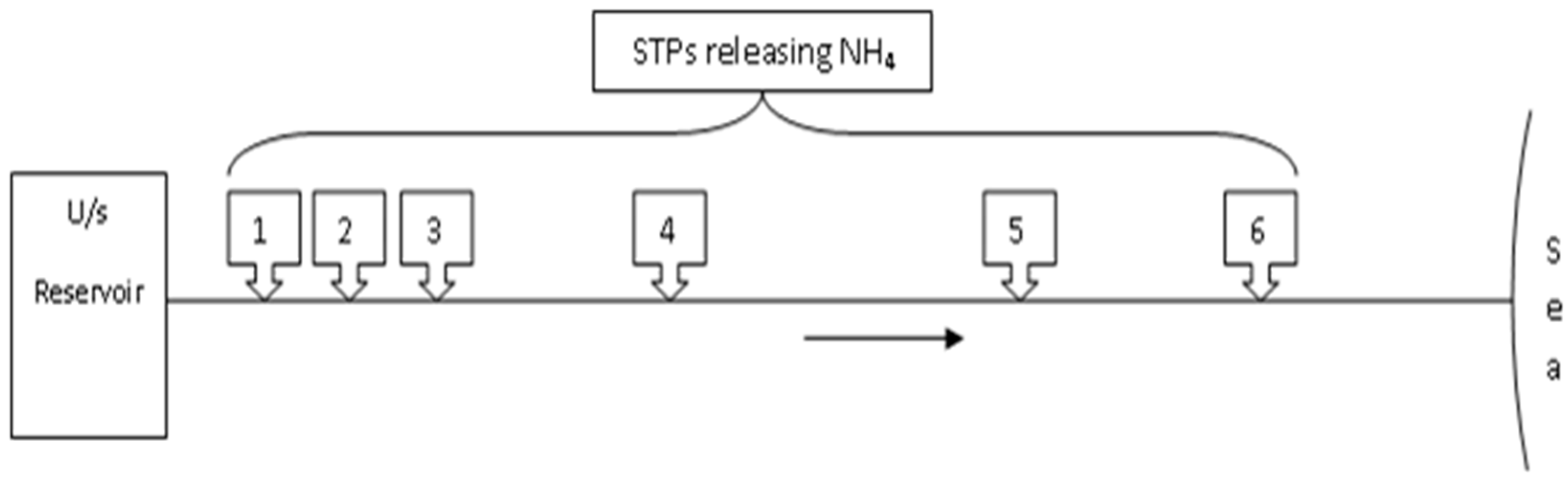
The present study aims at developing management models to control N2O emissions in a tidal river by determining optimal levels of wastewater treatment at different STPs discharging treated wastewater into the river, and also optimal releases from an upstream environmental reservoir for specified channel characteristics and tidal variation at the downstream end (Figure 3). Three different Management Models are proposed as described below.
2.3.1. Management Model-I (MM-I)
Management Model-I minimises the total operating cost of treatment during a specified duration, with an upper limit on total N2Oemission from the river during that period.
Decision Vector
Treatment levels, fj,k
fj,k indicates the fraction by which ammonium concentration should be brought down at the STP. j = 1, 2 … Nj indicates location of STPs; k = 1, 2 indicates time segment. k = 1 indicates high tide period and k = 2 indicates low tide period. The treatment levels during the high and low tide periods are taken differently because flow conditions are different. The residual ammonium concentration in the effluent of any STP is thus given by:
where, = ammonium concentration in the effluent from jth STP during kth time period and = ammonium concentration in the influent to the jth STP.
Objective Function
In MM-I, the objective is to minimise the total treatment cost.
Minimise:
ucost,N = unit cost of one kilogram of ammonium removal in INR; DT = time period in each time segment = 12 h. ND = number of days of operation. In the present study ND = 2 days.
Constraints
- Constraint on emission: The total amount of N2O emission from the entire river during the operation horizon, should be lesser than a maximum specified value, .is calculated as summation of N2O emissions at each location i along the length of the river over each time step .where, = rate of nitrogen emission from a single reach of length Δx in mg/L/s during the time period of Δt, = surface area of the reach = and hi,t = average depth in the reach. is calculated using the Equation (12).
- Simulation constraint: The concentration of N2O in any reach “i” at any instant “t” depends on upstream release of water, tidal variation, channel characteristics, and concentration of ammonium in the effluent from STPs discharging into the river.
- Treatment limits: There may be upper and lower limits for treatment fraction at STPs. Lower limit represents a completely untreated case, and the upper limit represents a maximum possible efficiency of ammonium removal in STP based on practical conditions [40].
2.3.2. Management Model-II (MM-II)
Management Model-II also deals with cost minimisation. If upstream water is not freely available, its cost should also be included in the total cost while minimising the cost. Hence, decision making should consider upstream release during the period of operation as a decision variable. The upstream release during the high tide period could be different from that during the low tide period. Constraints should reflect upper and lower limits to the water released from upstream. Details of MM-II are given below.
Decision Vector
Treatment levels, fj,k, for all locations j and k = 1, 2; upstream water release, Qu,k for k = 1, 2.
Objective Function
In MM-II, the objective is to minimise the total treatment cost plus cost of f water released above a minimum flow .
Minimise:
= unit cost of water per cubic meter in INR; = Minimum environmental flow maintained in the river for the ecological functioning of the river, m3/s.
Constraints
- Constraint on emission
- Simulation constraint
- Treatment limits
- Reservoir release constraint: Upstream reservoir release at any time should not be lesser than a minimum value, Qmin and not more than a maximum value, Qmax.
2.3.3. Management Model-III (MM-III)
Management Model-III minimises total N2O emission from the river during the specified duration of operation, with an upper limit on the total cost of operation during the specified duration.
Decision Vector
Treatment levels, fj,k, for all locations j and k = 1, 2; upstream water release, Qu,k for k = 1, 2.
Objective Function
Minimise:
Constraints
is the maximum allowable total cost during the time horizon for operation.
Above optimisation models MM-I, MM-II and MM-III were solved in a simulation-optimisation framework using the Simulated Annealing technique. Details of the solution technique have been presented earlier [33,34] and therefore are not repeated here. The inequality constraints on in MM-I and MM-II, and on in MM-III are handled using the Penalty function approach.
Penalty factor depends on the ratio of constraint violation in an exponential way.
3. Results and Discussion
The proposed management model can be used for water quality management in tidal rivers. This model suggests the extent of treatment for NH4+ in various STPs located along the banks of the river and discharging treated domestic wastewater into the river. The aim is to control nitrous oxide emissions from the river. Applicability of management models is illustrated here through proof-of-the-concept test cases. Although hypothetical proof-of-the-concept situations were considered here for STP locations and operations, the river characteristics, the flow conditions and the reaction rate constants in the transport model were near realistic and corresponded to those for the Tyne River.
It was hypothesised that six STPs were located along the river at 4, 6, 8, 13, 23 and 27 km from upstream tidal limit, releasing partially treated/ untreated effluent containing at a uniform rate of 0.1 m3/s. The input ammonium concentration at the inlet of for all STPs is 50 mg/L. At the upstream end of the river, it was assumed that a reservoir controlled the water release into the river. The total time horizon for operation and for computing N2O emission was taken over two days. The unit treatment cost for NH4+ was equal to INR 132.5/kg-N [41].
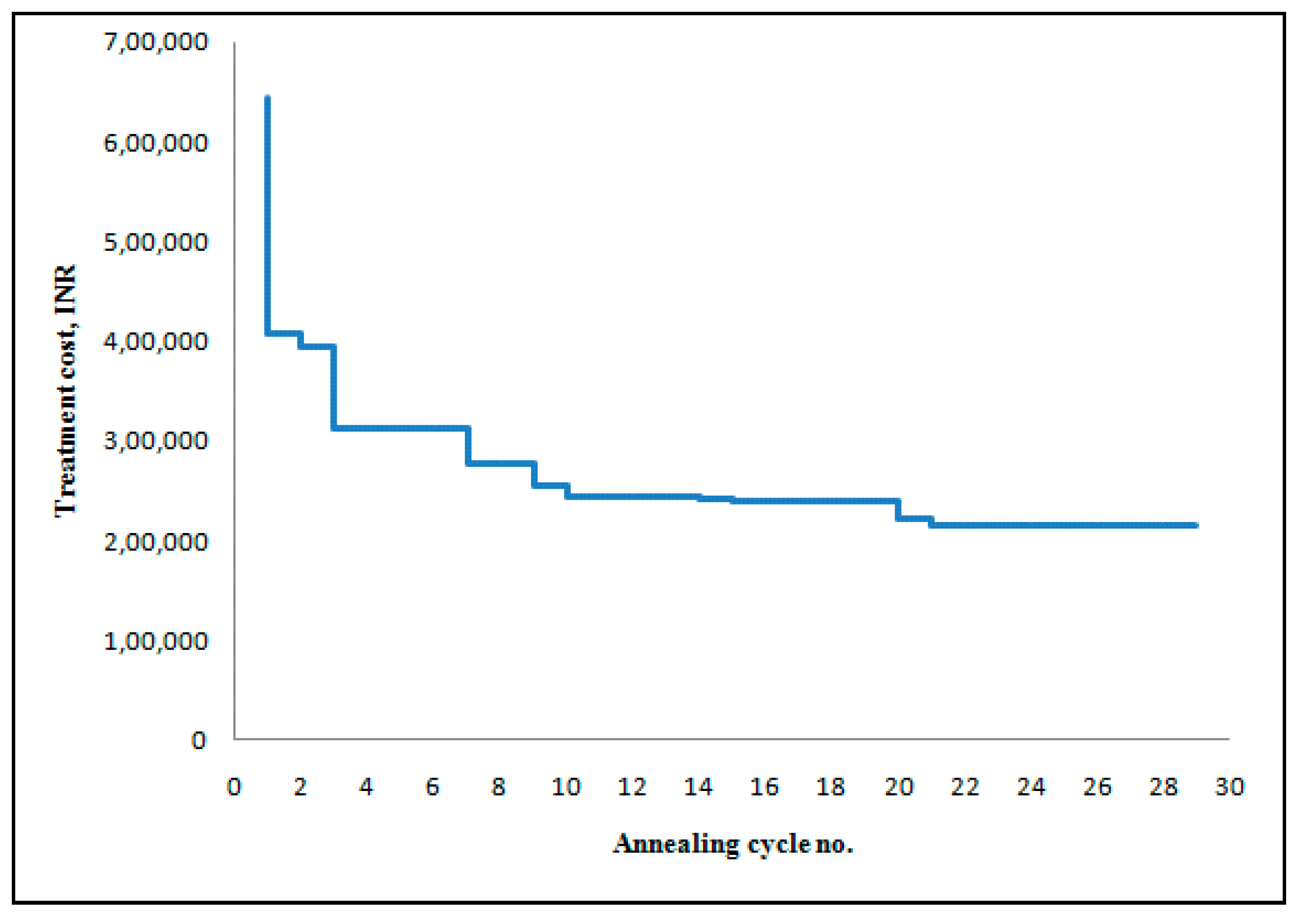
In the annealing process, initial temperature, number of iterations for each temperature and the temperature reduction factor were 1000, 50, and 0.8, respectively. The number of temperature reductions was based on attainment of the optimal solution. The terminal criterion was assumed to be met when there was no improvement of solution for five or more successive temperature reductions as shown in Figure 4, which depicts a typical evolution of objective function during Simulated Annealing (SA) optimisation solution. Herein, the objective function is the treatment cost. It may be noted that “temperature” that is referred to here is not the physical temperature but a numerical parameter in the SA technique for optimization [33,34]. Figure 4 indicates 29 annealing cycles and correspondingly 28 temperature reductions.
3.1. Illustration of Manage Model-I (MM-I)
All STPs were assumed to receive an input ammonium concentration of 50 mg/L, which is within the usual range for domestic wastewater. The six STPs continuously released effluents into the river at a rate of 0.1 m3/s. The upstream reservoir released a constant flow of 10 m3/s. The limiting nitrous oxide emission, , was taken as mean of N2O that would be released when complete treatment is given and when zero treatment is given at all the treatment plants.
Case 1: Constant treatment level throughout the time period
In this case, treatment fraction value at any STP was kept constant throughout the total time. So, for the 6 STPs the number of decision variables was six. The limiting N2O emission in two days was 189.8 g. Application of MM-1 provided the optimal solution as presented in Table 1.
A high treatment at 4 km and a moderate treatment at 8 km were needed to keep the N2O emission within limits. At 6 km and 13 km lower treatments were needed. Almost no treatment was needed at 23 km and 27 km. Provision of high treatment at 4 km resulted in lesser loading into the river and hence lesser transport of unoxidised NH4+ to the downstream. This justifies low treatment need at 6 km. Low treatment needs at treatment plants located in the lower stretches resulted because of lesser residential time for contaminant before it reached the sea.
Case 2: Different treatment levels during high and low tides
For a given loading, the transport of contaminant toward the sea is facilitated during the low tide, while it is hindered during the high tide. With increasing seaward transport and reduction in the residence time, the emission of N2O could be lower, and therefore a lower treatment effort during low tide would have sufficed to keep the total N2O emission within limits. This hypothesis was tested in Case-2 by applying different treatment levels during high and low tide periods. Thus, in Case-2, the total number of decision variables were 12, double as that in Case-1. Results corresponding to optimal solution for Case-2 are presented in Table 1.
Comparison of results for Case-1 and Case-2, presented in Table 1, clearly shows that for the same amount of nitrous oxide emission, the optimal cost in Case-2 was lesser by 35% as compared to the optimal cost in Case-1. During high tide, NH4+ would stay in the river for more time and therefore higher treatment was required, especially at STPs in the downstream reaches. A summation of treatment fractions during high tide for Case-2 was 2.3 as compared to 2.07 for Case-1 is given. The flow towards the sea during low tide helps in flushing more NH4+ downstream, so lesser treatment was needed for limiting total emission during the time period under consideration. A summation of treatment fractions during low tide for Case-2 was 0.34 as compared to 2.07 for Case-1 is given. Thus, it is clear that the treatment level at any STP should be varied during high and low tides in order to reduce the cost of operation, without crossing the limits for N2O emission.
Case 3: Effect of upstream release on optimal treatment cost
The amount of treatment that is required at the treatment plant in order to keep the emissions from the river below a specified level depends upon the flow rate in the river. However, it may be noted that flushing of ammonium towards the downstream may increase nitrous oxide emissions from the continental shelf. Herein it is assumed that reducing the nitrous oxide emission from the river and estuary is more important than reducing the export of ammonium to the continental shelf. This assumption is based on the study by Kroeze and Seitzinger [16] which estimated that global N2O emissions from continental shelves are expected to be affected majorly by changes in DIN inputs in estuaries and rivers.
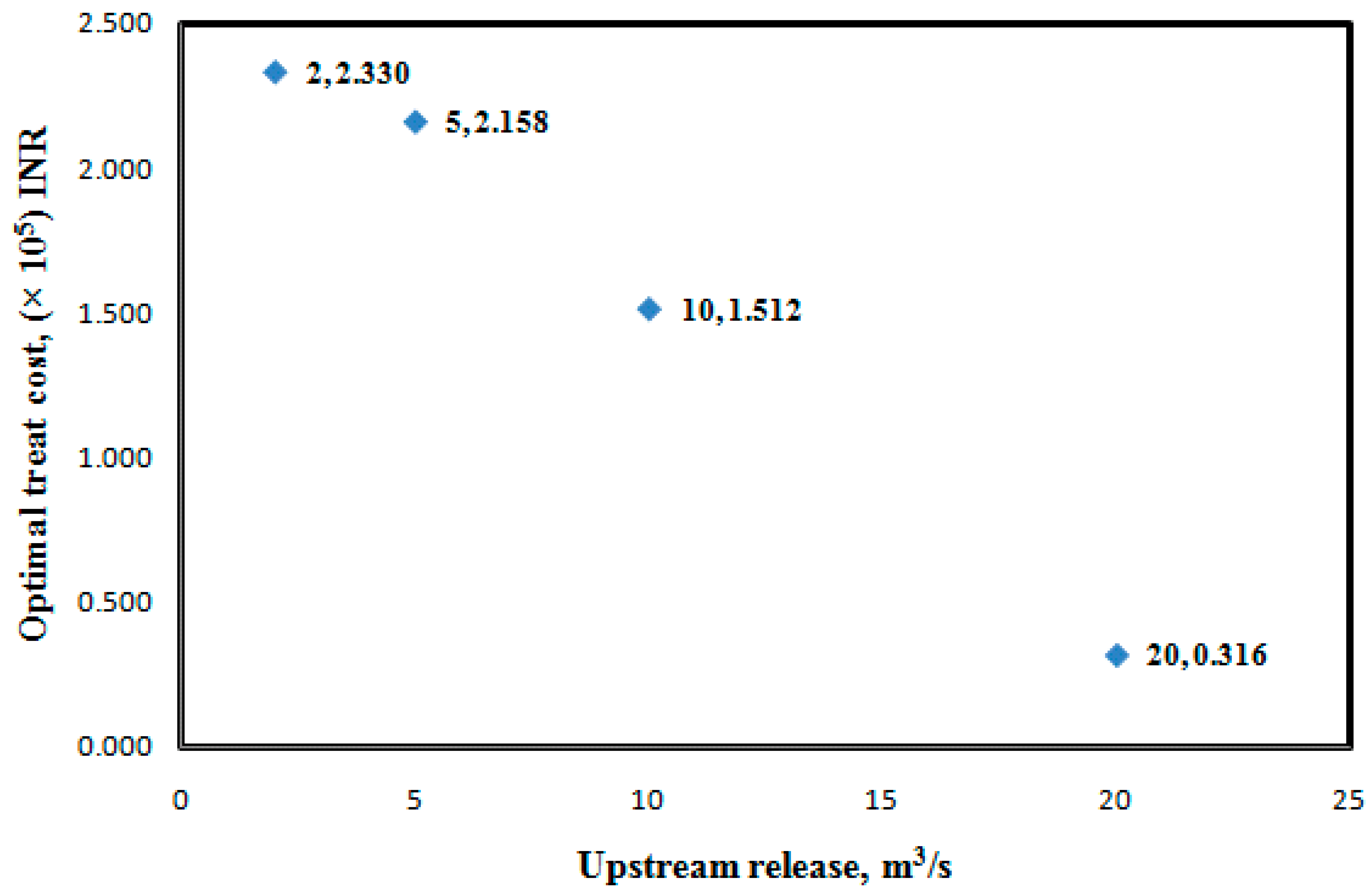
Proposed management model MM-I was used for studying the effect of upstream release on the optimal treatment cost. N2O emission was limited to the same value as in MM-1. Numerical runs were made for four different upstream releases of 2.0 m3/s, 5.0 m3/s, 10.0 m3/s and 20.0 m3/s for minimizing the treatment cost. Variation in the optimal treatment cost with upstream release is presented in Figure 5. It can be observed from Figure 5 that optimal treatment cost decreased almost linearly with the increase in upstream release. The treatment cost reduced from INR 2.330 × 10⁵ to INR 0.316 × 10⁵ as the upstream release increased from 2.0 m3/s to 20 m3/s. High water release rate from upstream side helped in dilution. It also reduced the residence time of the effluent, thereby resulting in reduction in nitrification, the N2O generation and emission from the river. These had a bearing on how much treatment was required at the treatment plants.
3.2. Illustration of Manage Model-II (MM-II): Case-IV and Case-V
Results from Section 3.1 indicate that one way of minimising the GHG emissions from the river due to contaminant loading is to maintain a high flow rate from the upstream end. However, the flow rate in a river may vary with seasons and may be quite low during certain periods of the year. In such cases, one can think of constructing an environmental reservoir at the upstream end, and regulate the releases from such a reservoir in order to reduce the GHG emissions. As explained earlier, this possibility was considered in MM-II, wherein the upstream release, Qu was treated as one of the decision variables. There was a lower limit to Qu, based on the requirement of minimum environmental flows (Qmin) to maintain river health. Any release over and above this minimum flow, for the purpose of minimising the emissions, carried a price. This cost was associated with the releases because that water could have been used for some other beneficial purpose. Therefore, the total cost, which was equal to the treatment cost plus the cost of water, was minimised by MM-II.
In Case-4, management model MM-II was run with Qmin = 5.0 m3/s. Input data for this case was the same as that for Case-2, but with Qu during low and high tide periods as additional decision variables. Therefore, the number of decision variables was equal to 14. The cost of water was taken from the range of water price for agriculture [42] (FAO, 2001). Two different values of water cost equal to INR 0.01 and INR 0.1 per cubic meter of water were considered to study the effect of water cost on the optimal solution. In Case-5, management model, MM-II was run with Qmin = 10.0 m3/s. Results of the optimisation runs for Case-4 and Case-5 are presented in Table 2. It can be observed from Table 2 that treatment was mostly needed only at the three upstream discharge points and only during high tide. Most of the total cost was incurred as water cost when water was priced at INR 0.01/m3 and the upstream release was high (Qu during high tide = 20 m3/s). However, as the price of water increased, the amount of water released from upstream reservoir decreased (Qu during high tide = 6.63 m3/s) and the treatment of wastewater at discharge locations increased in order to keep the emissions within limits. Results from Table 2 also indicate the effect of Qmin on the releases and the optimal cost. Almost no treatment was needed during the low tide when Qmin = 10 m3/s. It can be seen that optimal cost for Case-4a was equal to INR 1.12 × 10⁵ and for Case-4b, it was equal to INR 1.55 × 10⁵ which were much lesser in comparison with optimal treatment cost of INR 2.16 × 10⁵ when the upstream release was constant and equal to the minimum flow requirement of Qu = 5.0 m3/s. Similarly, optimal cost for Case-5 was equal to INR 1.29 × 10⁵ as compared to the total cost of INR 1.55 × 10⁵ when the upstream release was constant and equal to the minimum flow requirement of Qu = 10.0 m3/s. There was a 16.7% decrease in the cost. These results indicate that the dilution technique can be used for reducing the N2O emissions from the river, in addition to treating the inflowing wastewater, for achieving economical solutions.
3.3. Illustration of Manage Model-III (MM-III)
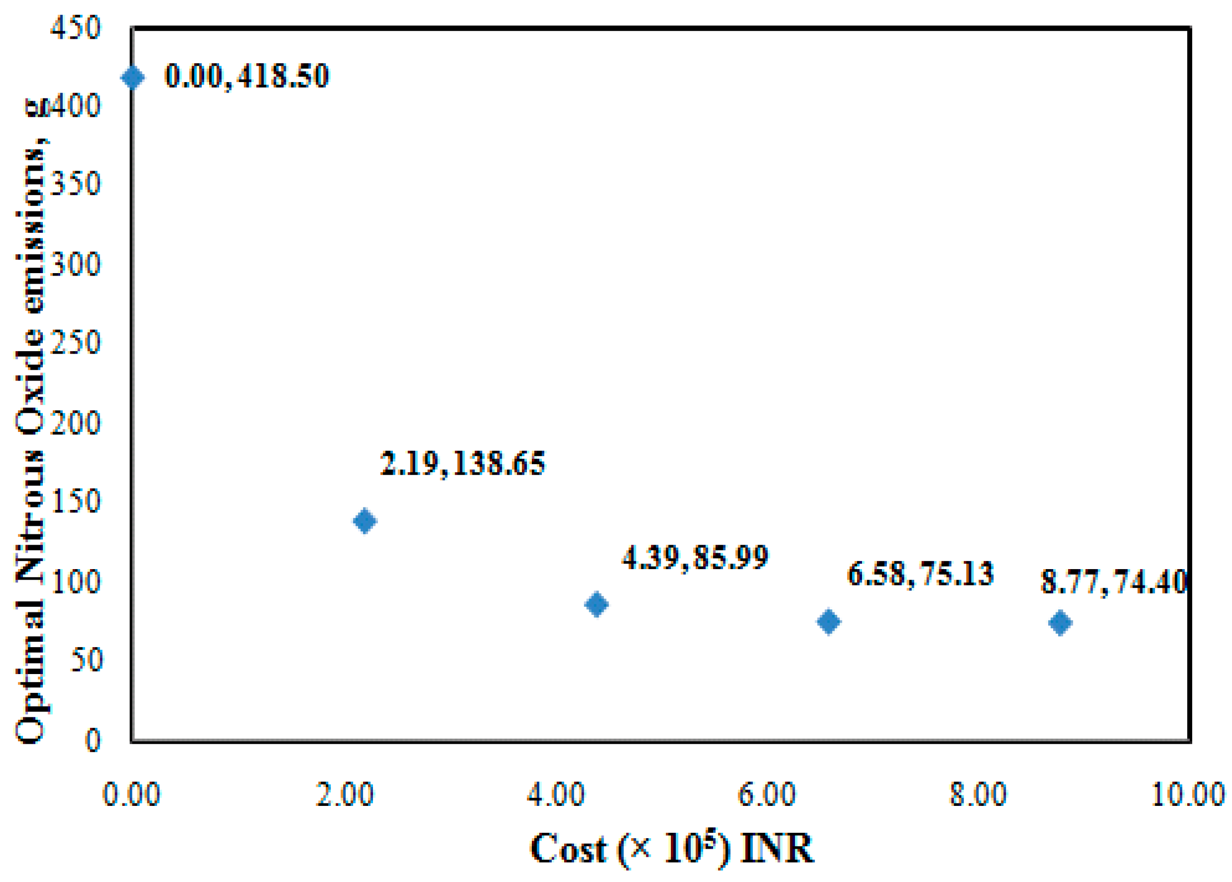
Case-6 illustrates the application of Management Model-III, which considered the minimisation of nitrous oxide emissions while keeping the total cost of treatment and water within limits. As in the Case-4, the total number of decision variables in Case-6 was 14. Also, the input for the Case-6 was the same as that for the Case-4. The minimum release, Qmin was equal to 5.0 m3/s and the cost of water was equal to INR 0.1/m3. Numerical runs were made for three different limiting costs equal to INR 2.2 × 10⁵, INR 4.4 × 10⁵ and INR 6.6 × 10⁵. The maximum emission, corresponding to no treatment and minimal release of water from upstream reservoir, was equal to 418.5 g per two days, at a zero cost. The minimum emission, corresponding to maximum treatment of 90% of incoming waste water and upstream release of 20 m3/s, was equal to 74.4 g per two days, at a cost of INR 8.77 × 10⁵. Results for minimum N2O emissions obtained using MM-III for different constraints on the maximum available money for treatment and water release are shown in Figure 6. The optimal operating schedule for different limiting costs is shown in Table 3. Table 3 also shows the percentage of the total cost that is spent on water release. As may be expected, one can reduce the amount of N2O emission from the river by spending more money on treatment and water release. If the amount available is less (INR 2.2 × 10⁵), it is better to spend a higher fraction of this money on water release rather than the treatment of wastewater to achieve the same level of N2O emissions. On the contrary, if the amount available is high (INR 6.6 × 10⁵), it is better to spend a higher fraction of this money on treatment rather than on water release. It can also be noted from Figure 6 that there is a limit to reduction in N2O emissions as one increases the amount of money spent on treatment and water release. Table 3 shows an observation that as the limiting cost increases, water release cost contribution to the total cost increased.
4. Conclusions
A simulation-optimisation management model was developed in this study to help managerial decisions for controlling nitrous oxide emissions from a tidal river through treating the incoming wastewater at different locations along the river and releases from an upstream reservoir. Management model coupled an advection-dispersion-reaction model to a penalty function-based simulated annealing algorithm for optimisation. Three management models were developed. Management model-I controlled the emissions by treating the incoming wastewater. Management model-II controlled the emissions by not only treating the incoming wastewater but also through managing the upstream releases. In both these models, the objective function dealt with minimisation of cost. Management model-III minimised the emissions through optimal operation when there was a constraint on the money available. Performances of the management models were demonstrated through proof-of-concept hypothetical scenarios for contaminant loading, but for realistic flow conditions corresponding to the Tyne River, UK. It was found that the treatment cost could be reduced by treating wastewater discharges joining the river more on the upper reaches and during the high tide. For the same level of N2O emissions, lesser costs could be achieved by not only treating the wastewater but also inducing dilution by releasing more water from the upstream side. It was also found that there was a limit to reduction in N2O emissions as one increased the amount of money spent on treatment and water release. The proposed management models will help to take the best decisions for controlling nitrous oxide emissions from tidal rivers.
Supplementary Materials
The following are available online at https://www.mdpi.com/2073-4441/11/6/1255/s1, Table S1: Width data and Initial Bathymetry of Tyne river, Table S2: Harmonic components of the tide, Table S3: Field measured inputs for Tyne River, Table S4: Longitudinal dispersion coefficient components.
Author Contributions
Conceptualization, C.A. and S.B.; Data curation, C.A.; Formal analysis, C.A. and S.B.; Funding acquisition, S.B.; Investigation, C.A.; Methodology, C.A. and S.B.; Project administration, S.B.; Resources, S.B.; Software, C.A. and S.B.; Supervision, S.B.; Validation, C.A. and S.B.; Visualization, C.A. and S.B.; Writing—original draft, C.A.; Writing—review and editing, S.B.
Funding
This research was funded by Department of Science and Technology (DST), India, grant number DST/TM/WTI/WIC/2K17/82(G).
Acknowledgments
The authors are very much thankful to Rodrigues, Polytechnic Institute of the State University of Rio de Janeiro, for providing us with the input hydraulic and contaminant data regarding their study on River Tyne, UK without which this work would not have been possible. Authors also thank Ligy Philip, IIT Madras for the many fruitful discussions.
Conflicts of Interest
The authors declare no conflict of interest.
References
- Forster, P.; Ramaswamy, V.; Artaxo, P.; Berntsen, T.; Betts, R.; Fahey, D.W.; Haywood, J.; Lean, J.; Lowe, D.C.; Myhre, G.; et al. Changes in Atmospheric Constituents and in Radiative Forcing; Solomon, S., Qin, D., Manning, M., Marquis, M., Averyt, K., Tignor, M.M.B., LeRoy Miller, H., Jr., Chen, Z., Eds.; Cambridge University Press: Cambridge, UK, 2007; p. 234. [Google Scholar]
- Galloway, J.N. The global nitrogen cycle: Changes and consequences. Environ. Pollut. 1998, 102 (Suppl. 1), 15–24. [Google Scholar] [CrossRef]
- Battle, M.; Bender, M.; Sowers, T.; Tans, P.; Butler, J.; Elkins, J.; Ellis, J.; Conway, T.; Zhang, N.; Lang, P. Atmospheric gas concentrations over the past century measured in air from firn at the South Pole. Nature 1996, 383, 231. [Google Scholar] [CrossRef]
- Steinfeld, H.; Gerber, P.; Wassenaar, T.; Castel, V.; Rosales, M.; De Haan, C. Livestock’s Long Shadow—Environmental Issues and Options; Food and Agriculture Organization (FAO) of the United Nations: Rome, Italy, 2006. [Google Scholar]
- Nitrous Oxide Emissions. U.S. Environmental Protection Agency. 2016. Available online: https://www.epa.gov/ghgemissions/overview-greenhouse-gases#nitrous-oxide (accessed on 11 April 2019).
- Kumar, S.; Smith, S.R.; Fowler, G.; Velis, C.; Kumar, S.J.; Arya, S.; Rena; Kumar, R.; Cheeseman, C. Challenges and opportunities associated with waste management in India. R. Soc. Open Sci. 2017, 4, 160764. [Google Scholar] [CrossRef] [PubMed] [Green Version]
- McMahon, P.; Dennehy, K. N2O emissions from a nitrogen-enriched river. Environ. Sci. Technol. 1999, 33, 21–25. [Google Scholar] [CrossRef]
- Marzadri, A.; Tonina, D.; Bellin, A.; Tank, J. A hydrologic model demonstrates nitrous oxide emissions depend on streambed morphology. Geophys. Res. Lett. 2014, 41, 5484–5491. [Google Scholar] [CrossRef] [Green Version]
- Beaulieu, J.J.; Nietch, C.T.; Young, J.L. Controls on nitrous oxide production and consumption in reservoirs of the Ohio River Basin. J. Geophys. Res. Biogeosci. 2015, 120, 1995–2010. [Google Scholar] [CrossRef] [Green Version]
- Middelburg, J.J.; Nieuwenhuize, J.; Iversen, N.; Høgh, N.; De Wilde, H.; Helder, W.; Seifert, R.; Christof, O. Methane distribution in European tidal estuaries. Biogeochemistry 2002, 59, 95–119. [Google Scholar] [CrossRef]
- Rajkumar, A.N.; Barnes, J.; Ramesh, R.; Purvaja, R.; Upstill-Goddard, R. Methane and nitrous oxide fluxes in the polluted Adyar River and estuary, SE India. Mar. Pollut. Bull. 2008, 56, 2043–2051. [Google Scholar] [CrossRef]
- Liu, X.-L.; Bai, L.; Wang, Z.-L.; Li, J.; Yue, F.-J.; Li, S.-L. Nitrous oxide emissions from river network with variable nitrogen loading in Tianjin, China. J. Geochem. Explor. 2015, 157, 153–161. [Google Scholar] [CrossRef]
- Burgos, M.; Sierra, A.; Ortega, T.; Forja, J. Anthropogenic effects on greenhouse gas (CH4 and N2O) emissions in the Guadalete River Estuary (SW Spain). Sci. Total Environ. 2015, 503, 179–189. [Google Scholar] [CrossRef]
- Wang, L.; Zhang, G.; Zhu, Z.; Li, J.; Liu, S.; Ye, W.; Han, Y. Distribution and sea-to-air flux of nitrous oxide in the East China Sea during the summer of 2013. Cont. Shelf Res. 2016, 123, 99–110. [Google Scholar] [CrossRef]
- He, Y.; Wang, X.; Chen, H.; Yuan, X.; Wu, N.; Zhang, Y.; Yue, J.; Zhang, Q.; Diao, Y.; Zhou, L. Effect of watershed urbanization on N2O emissions from the Chongqing metropolitan river network, China. Atmos. Environ. 2017, 171, 70–81. [Google Scholar] [CrossRef]
- Kroeze, C.; Seitzinger, S.P. Nitrogen inputs to rivers, estuaries and continental shelves and related nitrous oxide emissions in 1990 and 2050: A global model. Nutr. Cycl. Agroecosyst. 1998, 52, 195–212. [Google Scholar] [CrossRef]
- Denman, K.L.; Brasseur, G.; Chidthaisong, A.; Ciais, P.; Cox, P.M.; Dickinson, R.E.; Hauglustaine, D.; Heinze, C.; Holland, E.; Jacob, D.; et al. Couplings Between Changes in the Climate System and Biogeochemistry. Chapter 7; IPCC Working Group I, National Oceanic and Atmospheric Administration NOAA, DSRC R/AL/8, 325 Broadway, Boulder, CO 80305 (United States); Cambridge University Press: Cambridge, UK, 2007; pp. 499–587. [Google Scholar]
- Musenze, R.S.; Werner, U.; Grinham, A.; Udy, J.; Yuan, Z. Methane and nitrous oxide emissions from a subtropical estuary (the Brisbane River estuary, Australia). Sci. Total Environ. 2014, 472, 719–729. [Google Scholar] [CrossRef] [PubMed]
- Hu, B.; Wang, D.; Zhou, J.; Meng, W.; Li, C.; Sun, Z.; Guo, X.; Wang, Z. Greenhouse gases emission from the sewage draining rivers. Sci. Total Environ. 2018, 612, 1454–1462. [Google Scholar] [CrossRef] [PubMed]
- Cébron, A.; Garnier, J.; Billen, G. Nitrous oxide production and nitrification kinetics by natural bacterial communities of the lower Seine river (France). Aquat. Microb. Ecol. 2005, 41, 25–38. [Google Scholar] [CrossRef]
- Akbarzadeh, Z.; Laverman, A.M.; Rezanezhad, F.; Raimonet, M.; Viollier, E.; Shafei, B.; Van Cappellen, P. Benthic nitrite exchanges in the Seine River (France): An early diagenetic modeling analysis. Sci. Total Environ. 2018, 628, 580–593. [Google Scholar] [CrossRef] [PubMed]
- Radwan, M.; Willems, P.; El-Sadek, A.; Berlamont, J. Modelling of dissolved oxygen and biochemical oxygen demand in river water using a detailed and a simplified model. Int. J. River Basin Manag. 2003, 1, 97–103. [Google Scholar] [CrossRef]
- Chapra, S.C.; Pelletier, G.J.; Tao, H. QUAL2K: A Modeling Framework for Simulating River and Stream Water Quality, Version 2.11; Documentation and Users Manual; Department of Civil and Environmental Engineering, Tufts University: Medford, OR, USA, 2008. [Google Scholar]
- Ambrose, R.B.; Wool, T.A. WASP7 Stream Transport. Model. Theory and User’s Guide; U.S. Environmental Protection Agency: Athens, Greece, 2009.
- Regnier, P.; O’kane, J.; Steefel, C.; Vanderborght, J.-P. Modeling complex multi-component reactive-transport systems: Towards a simulation environment based on the concept of a Knowledge Base. Appl. Math. Model. 2002, 26, 913–927. [Google Scholar] [CrossRef]
- Rodrigues, P.; Barnes, J.; Upstill-Goddard, R. Simulating estuarine nitrous oxide production by means of a dynamic model. Mar. Pollut. Bull. 2007, 54, 164–172. [Google Scholar] [CrossRef]
- Garnier, J.; Billen, G.; Cébron, A. Modelling nitrogen transformations in the lower Seine river and estuary (France): Impact of wastewater release on oxygenation and N2O emission. Hydrobiologia 2007, 588, 291–302. [Google Scholar] [CrossRef]
- Burn, D.H.; Yulianti, J.S. Waste-load allocation using genetic algorithms. J. Water Resour. Plan. Manag. 2001, 127, 121–129. [Google Scholar] [CrossRef]
- Maier, H.R.; Lence, B.J.; Tolson, B.A.; Foschi, R.O. First-order reliability method for estimating reliability, vulnerability, and resilience. Water Resour. Res. 2001, 37, 779–790. [Google Scholar] [CrossRef] [Green Version]
- Mujumdar, P.P.; SubbaraoVemula, V. Fuzzy waste load allocation model: Simulation-optimization approach. J. Comput. Civ. Eng. 2004, 18, 120–131. [Google Scholar] [CrossRef]
- Yandamuri, S.; Srinivasan, K.; Murty Bhallamudi, S. Multiobjective optimal waste load allocation models for rivers using nondominated sorting genetic algorithm-II. J. Water Resour. Plan. Manag. 2006, 132, 133–143. [Google Scholar] [CrossRef]
- Mostafavi, S.A.; Afshar, A. Waste load allocation using non-dominated archiving multi-colony ant algorithm. Procedia Comput. Sci. 2011, 3, 64–69. [Google Scholar] [CrossRef] [Green Version]
- Belayneh, M.Z.; Bhallamudi, S.M. Optimization model for management of water quality in a tidal river using upstream releases. J. Water Resour. Prot. 2012, 4, 149. [Google Scholar] [CrossRef]
- Zewdie, M.; Bhallamudi, S.M. Multi-objective management model for waste-load allocation in a tidal river using archive multi-objective simulated annealing algorithm. Civ. Eng. Environ. Syst. 2012, 29, 222–230. [Google Scholar] [CrossRef]
- Niksokhan, M.; Ardestani, M. Multi-objective waste load allocation in river system by MOPSO. Int. J. Environ. Res. 2015, 9, 69–76. [Google Scholar]
- Nikoo, M.R.; Beiglou, P.H.B.; Mahjouri, N. Optimizing multiple-pollutant waste load allocation in rivers: An interval parameter game theoretic model. Water Resour. Manag. 2016, 30, 4201–4220. [Google Scholar] [CrossRef]
- Chaudhry, M.H. Open-Channel Flow, 2nd ed.; Springer: New York, NY, USA, 2008; p. 523. [Google Scholar]
- Broecker, W.S.; Peng, T.H. Tracers in the Sea; Eldigio Press: New York, NY, USA, 1982. [Google Scholar]
- Park, J.; James, A. A unified method of estimating longitudinal dispersion in estuaries. In Water Pollution Research and Control Brighton; Elsevier: Amsterdam, The Netherlands, 1988; pp. 981–993. [Google Scholar]
- Delgadillo-Mirquez, L.; Lopes, F.; Taidi, B.; Pareau, D. Nitrogen and phosphate removal from wastewater with a mixed microalgae and bacteria culture. Biotechnol. Rep. 2016, 11, 18–26. [Google Scholar] [CrossRef] [PubMed]
- Stare, A.; Vrečko, D.; Hvala, N.; Strmčnik, S. Comparison of control strategies for nitrogen removal in an activated sludge process in terms of operating costs: A simulation study. Water Res. 2007, 41, 2004–2014. [Google Scholar] [CrossRef] [PubMed]
- Cornish, G.; Bosworth, B.; Perry, C.; Burke, J.J. Water Charging in Irrigated Agriculture: An Analysis of International Experience; Food & Agriculture Organization: Rome, Italy, 2004; Volume 28. [Google Scholar]
Figure 1.
Comparison of current Simulations (continuous lines) and field measured values from Rodrigues et al, 2007 (solid circles) [26] of water level elevation about mean: (a) At 15 km; and (b) at 19 km from upstream end.
Figure 1.
Comparison of current Simulations (continuous lines) and field measured values from Rodrigues et al, 2007 (solid circles) [26] of water level elevation about mean: (a) At 15 km; and (b) at 19 km from upstream end.

Figure 2.
Comparison of current Simulations (continuous lines) and field measured values from Rodrigues et al, 2007 (solid diamonds) [26] of longitudinal profiles of mean monthly concentrations of: (a) NH4+, (b) NO3−, and (c) N2O for August 2000 in Tyne river.
Figure 2.
Comparison of current Simulations (continuous lines) and field measured values from Rodrigues et al, 2007 (solid diamonds) [26] of longitudinal profiles of mean monthly concentrations of: (a) NH4+, (b) NO3−, and (c) N2O for August 2000 in Tyne river.

Figure 3.
Schematic diagram for management models.

Figure 4.
The typical evolution of objective function during the optimisation solution.

Figure 5.
Optimal cost for different upstream releases.

Figure 6.
Effect of limiting cost on optimal emissions.


Table 1.
Optimal operating schedule: Case-I.
| Location | 4 km | 6 km | 8 km | 13 km | 23 km | 27 km | N2O, g | Optimal Treatment Cost, INR | |
|---|---|---|---|---|---|---|---|---|---|
| Case-1 | HT | 0.88 | 0.27 | 0.54 | 0.34 | 0.00 | 0.04 | 188 | 236,593 |
| LT | 0.88 | 0.27 | 0.54 | 0.34 | 0.00 | 0.04 | |||
| Case-2 | HT | 0.66 | 0.73 | 0.41 | 0.16 | 0.10 | 0.24 | 188 | 151,280 |
| LT | 0.02 | 0.07 | 0.18 | 0.00 | 0.05 | 0.02 | |||
Table 2.
The optimal operating schedule for cost minimisation: Case-4 and Case-5.
| Qmin | Tidal Period | 4 km | 6 km | 8 km | 13 km | 23 km | 27 km | Qu, m3/s | Optimal Cost, INR | N2O, g | |
|---|---|---|---|---|---|---|---|---|---|---|---|
| 10 | 0.01 | HT | 0.61 | 0.04 | 0.00 | 0.02 | 0.02 | 0.05 | 18.42 | 54,637 | 188 |
| LT | 0.00 | 0.00 | 0.00 | 0.00 | 0.00 | 0.00 | 14.67 | ||||
| 0.1 | HT | 0.18 | 0.27 | 0.27 | 0.00 | 0.35 | 0.00 | 17.69 | 128,766 | 189 | |
| LT | 0.02 | 0.00 | 0.00 | 0.00 | 0.00 | 0.00 | 10.00 | ||||
| 5 | 0.1 | HT | 0.81 | 0.78 | 0.79 | 0.00 | 0.00 | 0.00 | 6.63 | 154,941 | 190 |
| LT | 0.00 | 0.00 | 0.00 | 0.02 | 0.00 | 0.00 | 5.28 |
Table 3.
The optimal operating schedule for Case-6.
| Limiting Cost (×105) INR | Tidal Ceriod | 4 km | 6 km | 8 km | 13 km | 23 km | 27 km | Qu, m3/s | Optimal N2O, g | % Water Cost |
|---|---|---|---|---|---|---|---|---|---|---|
| 6.6 | HT | 0.90 | 0.90 | 0.90 | 0.90 | 0.90 | 0.65 | 20.00 | 75.13 | 42 |
| LT | 0.31 | 0.57 | 0.55 | 0.10 | 0.11 | 0.44 | 7.68 | |||
| 4.4 | HT | 0.89 | 0.90 | 0.90 | 0.82 | 0.73 | 0.00 | 17.09 | 85.99 | 45 |
| LT | 0.00 | 0.31 | 0.27 | 0.85 | 0.00 | 0.01 | 5.29 | |||
| 2.2 | HT | 0.90 | 0.90 | 0.87 | 0.07 | 0.00 | 0.01 | 10.38 | 138.65 | 62 |
| LT | 0.00 | 0.00 | 0.06 | 0.00 | 0.00 | 0.10 | 5.00 |
© 2019 by the authors. Licensee MDPI, Basel, Switzerland. This article is an open access article distributed under the terms and conditions of the Creative Commons Attribution (CC BY) license (http://creativecommons.org/licenses/by/4.0/).
Share and Cite
MDPI and ACS Style
Akella, C.S.; Bhallamudi, S.M. Managing Municipal Wastewater Treatment to Control Nitrous Oxide Emissions from Tidal Rivers. Water 2019, 11, 1255. https://doi.org/10.3390/w11061255
AMA Style
Akella CS, Bhallamudi SM. Managing Municipal Wastewater Treatment to Control Nitrous Oxide Emissions from Tidal Rivers. Water. 2019; 11(6):1255. https://doi.org/10.3390/w11061255
Chicago/Turabian StyleAkella, Chandra Sekhar, and S. Murty Bhallamudi. 2019. "Managing Municipal Wastewater Treatment to Control Nitrous Oxide Emissions from Tidal Rivers" Water 11, no. 6: 1255. https://doi.org/10.3390/w11061255
Note that from the first issue of 2016, this journal uses article numbers instead of page numbers. See further details here.