Roughness Effect of Submerged Groyne Fields with Varying Length, Groyne Distance, and Groyne Types


1
Aller-Ohre-Verband, 38518 Gifhorn, Germany
2
Leichtweiß-Institut für Wasserbau, Technische Universitaet Braunschweig, 38106 Braunschweig, Germany
*
Author to whom correspondence should be addressed.
Water 2019, 11(6), 1253; https://doi.org/10.3390/w11061253
Submission received: 16 April 2019
/
Revised: 29 May 2019
/
Accepted: 11 June 2019
/
Published: 14 June 2019
(This article belongs to the Special Issue Water-Worked Bedload: Hydrodynamic and Mass Transport)
Abstract
:Design guidelines were developed for a number of in-stream structures; however, the knowledge about their morphological and hydraulic function is still incomplete. A variant is submerged groynes, which aim to be applicable for bank protection especially in areas with restricted flood water levels due to their shallow height. Laboratory experiments were conducted to investigate the backwater effect and the flow resistance of submerged groyne fields with varying and constant field length and groyne distance. The effect of the shape of a groyne model was investigated using two types of groynes. The validity of different flow types, from “isolated roughness” to “quasi smooth”, was analyzed in relation to the roughness density of the groyne fields. The results show a higher backwater effect for simplified groynes made of multiplex plates, compared to groynes made of gravel. The relative increase of the upstream water level was lower at high initial water levels, for short length of the groyne field, and for larger distance between the single groynes. The highest roughness of the groyne fields was found at roughness densities, which indicated wake interference flow. Considering a mobile bed, the flow resistance was reduced significantly.
1. Introduction
Many types of in-stream structures, e.g., stream barbs, bendway weirs, and different kinds of vanes and groynes, were developed aiming to comply with demands for both river training and restoration. An overview of types and related studies is given by Radspinner et al. [1] and, more recently, by Zaid [2]. Studies on ecological benefits e.g., [3], morphological effects e.g., [2,4,5,6,7,8,9,10], and flow fields [7,10,11,12,13,14,15] provide evidence of the structures’ potential. Single structures are often used for ecological purposes only, i.e., to increase the variation of river morphology and flow diversity in river restoration projects e.g., [4,10]. For nature-orientated river training, arrangements of groynes are employed, e.g., [2,3,13]. Both single elements and groups of structures require design guidelines for the stability of the structure itself, e.g., [4,5,6,9], as well as for the specific purpose of implementation. For specific structure types, mainly stream barbs and bendway weirs, design guidelines were developed based on field experience, e.g., [16,17], numerical simulations, e.g., [11], and physical model tests, e.g., [11,13,18]. However, the studies usually conclude that further investigations are required, demonstrating that still some design aspects are not considered.
A feature that cannot be fulfilled by the aforementioned structures is to leave flood water levels almost unaffected. Therefore, submerged groynes were developed for ecologically compatible bank protection especially in areas with restricted flood water levels [2,10,13]. The structure is characterized by a horizontal crest and a height related to the mean low water level at the implementation site. Thus, it is submerged over its full length almost throughout the year and supports the water level especially during low flow conditions. However, during floods the water level rise shall be limited to a minimum. Consequently, knowledge of the backwater height is of high relevance for these structures.
A groyne field can be represented as a large obstacle or a series of small weirs [19]. Yossef [19] considered the field as an obstacle, and developed a formula for calculating the bulk drag coefficient as a function of the blockage ratio and the Froude number, based on experiments with an immobile bed, one groyne setup, and different hydraulic conditions. For applying the formula on a different setup, the flow velocity above the groyne field and in the unblocked part of the cross-section need to be known. The experiments were conducted with nonuniform flow conditions, and thus conclusions cannot be drawn from presented drag force coefficients to assess the development of the backwater with the level of submergence.
Azinfar and Kells [20] investigated the backwater effect of a groyne field, which was simulated by thin plastic plates. They derived a formula relating the effect of the groyne field to the backwater effect of a single groyne. To apply the formula, the flow field caused by a single groyne (backwater height and velocity in that cross-section), its drag force coefficient, and the total relative drag force of the field have to be known. For the latter an empirical formula was provided considering the number of groynes. The effect of a varying groyne field length is implicitly included but not discussed. The authors point out that the formulas are only valid for thin plastic plates and hydraulic conditions within the investigated range (e.g., relative submergence from 1.2 to 2). Transferable findings are that the backwater increases with the number, the spacing of the plates, and increasing submergence, and that the flow resistance of a submerged groyne field is larger than that of a single plate. They concluded that their arrangements are in the wake-interference region following the concept of Morris [21], as the total drag forces were larger than the sum of drag forces caused by an according number of single groynes.
For roughness elements evenly distributed on the bed, Morris [21] distinguished the flow types quasi-smooth (or skimming), wake interference, and isolated roughness flow, which Chow [22] visualized in a sketch. Starting from a dense packing of the roughness elements, the flow resistance of the bed first increases with increasing spacing between the elements until a maximum is reached. For these arrangements, the wakes and vortices at each element interfere with those developed at the neighboring elements, resulting in intense and complex vorticity and turbulent mixing [22]. Further increase of the spacing results in decreasing flow resistance. The spacing can be parameterized by the roughness density ck, which is the ratio of the upstream projected area of an element to the floor area assigned to that element. According to analysis of numerous studies, the maximum flow resistance, i.e., wake interference flow starts to develop at ck = 0.1 and is maximum at ck between 0.2 and 0.35, e.g., [23,24]. Comparable results were found using the spatial density of roughness elements [25].
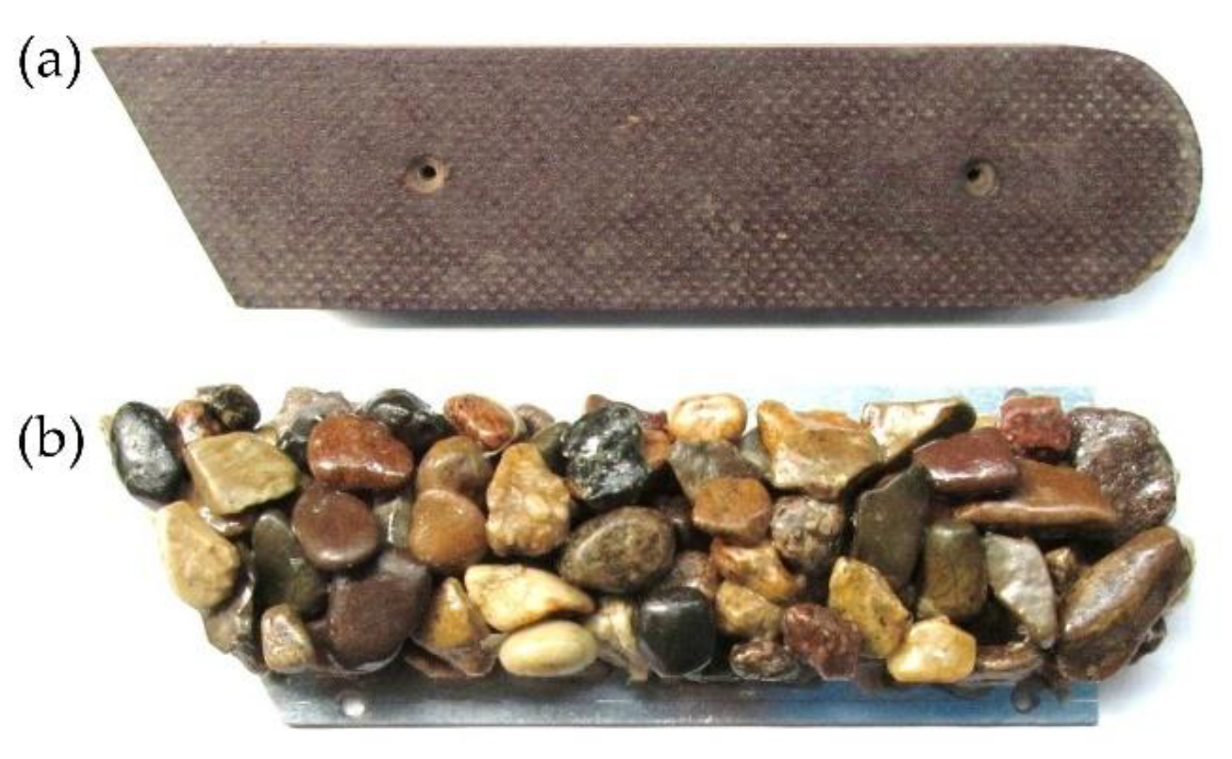
First, recommendations for designing a submerged groyne field for bank protection are given by Mende [13], based on studies in a straight laboratory flume with immobile bed and banks and a simple groyne model made of multiplex (Figure 1a). Möws and Koll [10] improved the groyne model (Figure 1b) and investigated morphological and hydraulic effects on a single submerged groyne in a straight laboratory flume with a mobile bed. In contrast to common results e.g., [5,6,9], the main scour at the groyne head is not attached to the groyne, but located further downstream, which is related to the groyne shape. A similar scouring effect due to the groyne shape was observed by Bressan and Papanicolaou [4] for stream barbs up to a certain level of submergence and by Kadota et al. [8] for permeable submerged groynes. Using the gravel groyne model (Figure 1b) for investigating the effect of geometric groyne parameters [26] and of the position of a submerged groyne [27] on the velocity field in a curved laboratory channel, which finally resulted in recommendations for arranging a submerged groyne field for protecting the outer bank of a bend [2]. However, only one hydraulic boundary condition was adjusted in the latter experiments and thus, the effect of a submerged groyne field on the water level cannot be estimated, yet.
The aim of the work described in this paper is to investigate the hydraulic roughness of fields of submerged groynes and to assess the effect of model boundary conditions. Using experiments with fixed beds, the effects of roughness density, groyne field length, and the level of simplification of a groyne model on the water level and the friction factor were analyzed. In order to assess the effect of morphological adaptations on the hydraulic roughness, an additional experiment was conducted with mobile bed conditions. Two different groyne models were used as well as varying groyne field lengths and groyne numbers and three levels of submergence. All experiments took place in the hydraulic laboratory of the Leichtweiß-Institute for Hydraulic Engineering and Water Resources.
2. Materials and Methods
The hydraulic roughness of a groyne field, depending on its length and the number of groynes, was investigated in two series of laboratory experiments. The first test series, GF 1, was conducted with a fixed number of groynes (15) and varying distance between the groynes (dG), resulting in different lengths of the groyne field (lGF). Two types of groynes (Figure 1) were compared: a simplified model of a groyne made of multiplex plates characterized by sharp edges with no sloping from crest to base and a flat top and a second type made from glued gravel (12–16 mm), which resulted in an irregular surface and a slightly permeable body.
In the second series of experiments, GF 2, the length of the groyne field was kept constant (1.5 m). Thus, varying the distance between the groynes resulted in different numbers of groynes. These experiments were conducted only with the gravel groynes.
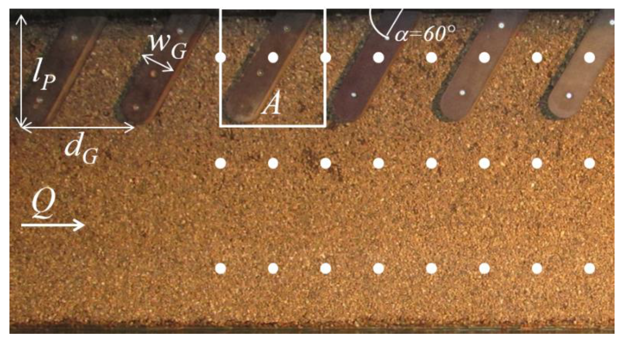
The fixed bed experiments were conducted in a 30 m long, 60 cm wide, and 70 cm deep hydraulic flume with walls made of glass. On the horizontal flume floor a second floor was built from plywood plates with a length of 15 m and a slope of 0.3%. A single layer of fine gravel (mean diameter dm = 3.64 mm) was glued on the plates to roughen the second floor. A flap gate was installed at the downstream end of the second floor for regulating the water level. The discharge (Q) was controlled by a valve and measured with an inductive discharge meter, and the water depth (h) was measured with a mobile point gauge. The groyne field was located on the left side of the flume always starting at x = 7 m (position of groyne toe), with the origin of the longitudinal coordinate x = 0 at the upstream end of the second floor. The upstream reach of 7 m length was chosen to ensure fully developed flow conditions. The groynes were installed on top of the rough bed. The groyne height (hG) of both groyne types was 2.5 cm to investigate relative submergence up to 6. The groyne width (wG) was 6 cm and the projected length of the groyne (lP) was 20 cm (1/3 of the flume width). The angle of inclination was chosen to 60° against stream direction (Figure 2) as several studies e.g., [13,18,26] recommend this angle for best protection of a bank.
In experiments without groynes, the boundary conditions for uniform flow conditions at water depths hN = 5, 10, and 15 cm were determined by adjusting the flap gate and the discharge until the target water depth was constant along the flume. The resulting relative submergence for the groyne experiments was 2, 4, and 6. The settings of in total 51 experiments are summarized in Table 1. The roughness density (ck) is calculated as the ratio of the projected area (A’), which is the product of the groyne height and the projected length, and the related ground area of a groyne (A, see Figure 2) (Equation (1)).
with m = number of groynes, dG = groyne distance, dG/lP = aspect ratio, lGF = groyne field length, ck = roghness density, hN = uniform flow water depth without groynes, Fr = Froude number, and Q = discharge.
In GF 1 the runs with the largest distance between the groynes were carried out with only 14 groynes because of the limited length of the second floor of 15 m.
Water levels were measured in three sections in flow direction: along the center of the groynes (10 cm distance to the left flume wall), along the middle of the flume, and in 10 cm distance to the right flume wall (Figure 2). The water depths were averaged over the cross-section to analyze the bulk effect of a groyne field.
The hydraulic roughness of a groyne field is parameterized by the Darcy–Weisbach friction coefficient f (Equation (2)). For the energy slope, the local energy height was determined by summing up the water depth, averaged across the flume, and the velocity height within each cross-section. The local mean flow velocities were calculated with the continuity equation. A linear trend was fitted to the energy heights starting at the cross-section with maximum water depth and ending at the first cross-section downstream of the groyne field. As the flume walls were much smoother than the flume bed, the hydraulic radius is replaced by the water depth hmax.
with hmax = maximum water depth along the flume, SE = energy slope, and um = mean flow velocity calculated with hmax.
The mobile bed experiment (GF 3) was carried out in a 90 cm wide and 60 cm deep tilting flume (slope = 0.3%). A 10-cm-thick layer of fine gravel (mean diameter dm = 3.64 mm) was placed over a length of 15 m in a 20-m-long flume. A set of ten gravel groynes, with a height of 2.5 cm and lP = 31 cm (approximately one-third of the flume width), was installed with dG = 20 cm, 60° angled against flow direction, resulting in ck = 0.125. The first groyne started at x = 8.35 m, with the origin of x being defined as the beginning of the sediment layer. The water depth at uniform flow conditions (without groynes) was set to 10 cm, which corresponded to incipient motion conditions for the bed material. The experiment ran for 7 hours until only minor changes of the bed topography were observed visually. The resulting bed topography was scanned with a high resolution laser scanner from x = 8 to 10.5 m and across the flume from y = 0.09 to 0.81 m. The resolution of the scan was 0.5 mm in the x-direction and 10 mm in the y-direction. Water levels were measured in three sections in flow direction, relatively related to those in the fixed bed experiments.
3. Results and Discussion
The effect of a groyne field on the water level along the flume was very similar for all experiments, and thus is shown exemplarily for one setup and the three hydraulic conditions in Figure 3. Throughout the experiments the highest increase of the water depth (Δh = hmax − hN) was located about 10 cm upstream of the groyne field at x = 6.9 m, which corresponded to the position of the first groyne head. Deviations in the exact longitudinal position of the maximum water depth were due to the wavy water surface, which became more predominant with increasing approach velocity, i.e., increasing hN, and to the fixed raster for water depth measurements with a distance of 10 cm. However, a difference between the water depth at x = 6.9 m and the maximum water depth was observed in only two experiments and was 3 and 4 mm, respectively. Thus, this position is used for further analysis. Towards the downstream end of the groyne field the water level decreased following a linear trend. As expected, the water level downstream of the last groyne was in general lower than hN. Despite the scatter due to waves, it is obvious that the backwater increased with increasing water depth hN. However, the rise of the backwater height at position x = 6.9 m decreased with increasing discharge, i.e., the difference of Δh was always larger from hN = 5 cm to 10 cm than from hN = 10 cm to 15 cm, indicating a diminishing effect of the groynes with increasing submergence.
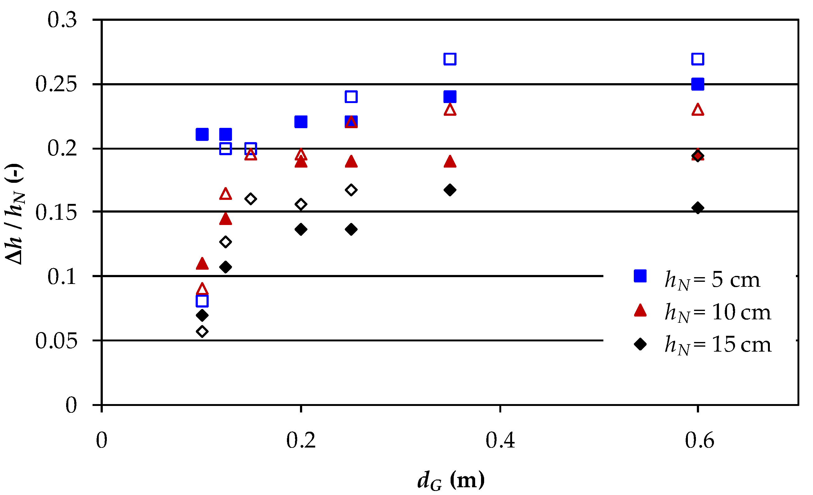
The influence of the hydraulic boundary conditions becomes evident by plotting the relative increase of the water depth (Δh/hN), measured at x = 6.9 m, which is presented in Figure 4 for the experimental series GF 1 (Table 1). The number of groynes was kept constant, and thus the length of a groyne field grew with the distance between the groynes. Accordingly, the backwater increased with the distance between the groynes; however, approaching a constant backwater height independent of dG and the groyne field length.
The change from a steep to an asymptotic increase of Δh/hN occurred at dG = 15 cm for the experiments with larger submergence. The projected width of a groyne (the distance between head and toe along the x-axis) was 11.55 cm. Thus, the head of a downstream groyne overlapped with or was very close to the toe of the upstream groyne for dG = 10 and 12.5 cm, resp., which can hinder the development of the overtopping flow, and thus result in lower flow resistance. This effect was observed throughout the experiments except for the gravel groynes with hN = 5 cm in series GF 1. However, this measured water level may be biased as it should match with the water level measured in the corresponding experiment in series GF 2 (see Figure 5).
Depending on the distance between groynes, the backwater height reached up to 25–27% of the undisturbed water depth for the lowest submergence (hN = 5 cm) and 15–19% for hN = 15 cm. The variation is mainly caused by the way of modeling a groyne. The multiplex groynes resulted in higher water depths than the gravel groynes, independent of the level of submergence. The impact was smaller for short distances between the groynes, and the reverse for the shortest groyne distance. The flow field caused by the smooth surface and the sharp edges of the multiplex groynes resulted in higher flow resistances than observed for the irregularly shaped surface and porous body of the gravel groynes. Thus, results from the experiments with strongly simplified substitutes, e.g., the multiplex groynes or plates used by Azinfar and Kells [20] overestimate the groyne influence.
In contrast to the asymptotic increase of the backwater in the experiments with a growing groyne field length (GF 1), the relative increase of the upstream water level reached a maximum, if the groyne field length was kept constant (GF 2) (Figure 5). Independent of the approach flow, the groyne distance dG = 15 cm resulted in the largest hydraulic roughness. With larger groyne distances the relative backwater decreased asymptotically. The minimum backwater can be expected to correspond to the effect of a single groyne.
Considering a groyne field as a large obstacle as Yossef [19] recommended, its roughness consists of two parameters: the groyne field length and the groyne density within the field. The different relationships, presented in Figure 6, show that the decreasing roughness due to a wider spacing was at least counterbalanced by the increasing roughness of a growing field length. This finding highlights the importance of considering not only the number and spacing of groynes, but of also taking the resulting total length of the groyne field into account. This is important especially for nature-oriented river training as these projects are often planned for river reaches with limited length.
For comparing the experiments with variable and fixed groyne field lengths the friction coefficient f was calculated with Equation (2) (Figure 6). The maximum flow resistance caused by a groyne field was found at dG = 12.5 and 15 cm, respectively, except for the test run in series GF 1 with gravel groynes and hN = 5 cm for the aforementioned reason. The multiplex groynes caused larger flow resistance than the gravel groynes. The setup with constant groyne field length (GF 2) resulted in larger friction factors than the setup with variable length (GF 1). However, the friction factors for multiplex and gravel groynes, especially for constant and variable groyne field lengths, followed the same trend. This indicates that the decrease of the energy slope with increasing groyne distance was more distinct for the variable groyne field length than for the constant one. Further investigations require more precise water level measurements to reduce the scatter due to the wavy water surface.
Groyne distances are related to roughness density ck, which is plotted as second x-axis in Figure 6. The maximum flow resistance corresponded to roughness densities between 0.17 and 0.2 indicating wake interference flow [23,24]. The difference to Canovaro et al. [25], who found maximum flow resistance for spatial densities between 0.2 and 0.4, can be explained with the element height, which is included in ck, but not in the spatial density.
The results show that the concept described by Morris [21] can be applied to the flow over a groyne field, even if the roughness elements are not distributed over the full width of the flume. This finding demonstrates the possibility to use the comprehensive knowledge of flow over rough surfaces to study the hydraulic effects of submerged groyne like structures.
The different backwater heights caused by the simplified multiplex models and the gravel groynes demonstrated that shape matters. For the backwater effect, an overestimation can be considered as positive, as the results would be conservative. However, if simple structures, especially those with sharp edges, are used in morphodynamic studies, misleading conclusions may be drawn. For example, studies of morphological changes due to simplified models report distinct scouring at the head of the groynes, e.g., [6,9]. On the contrary, in mobile bed experiments carried out with more naturally shaped types of single submerged groynes, the main scour was observed downstream of the groyne head [4,8,10] and the stability of the structure was not compromised by a groyne head scour.
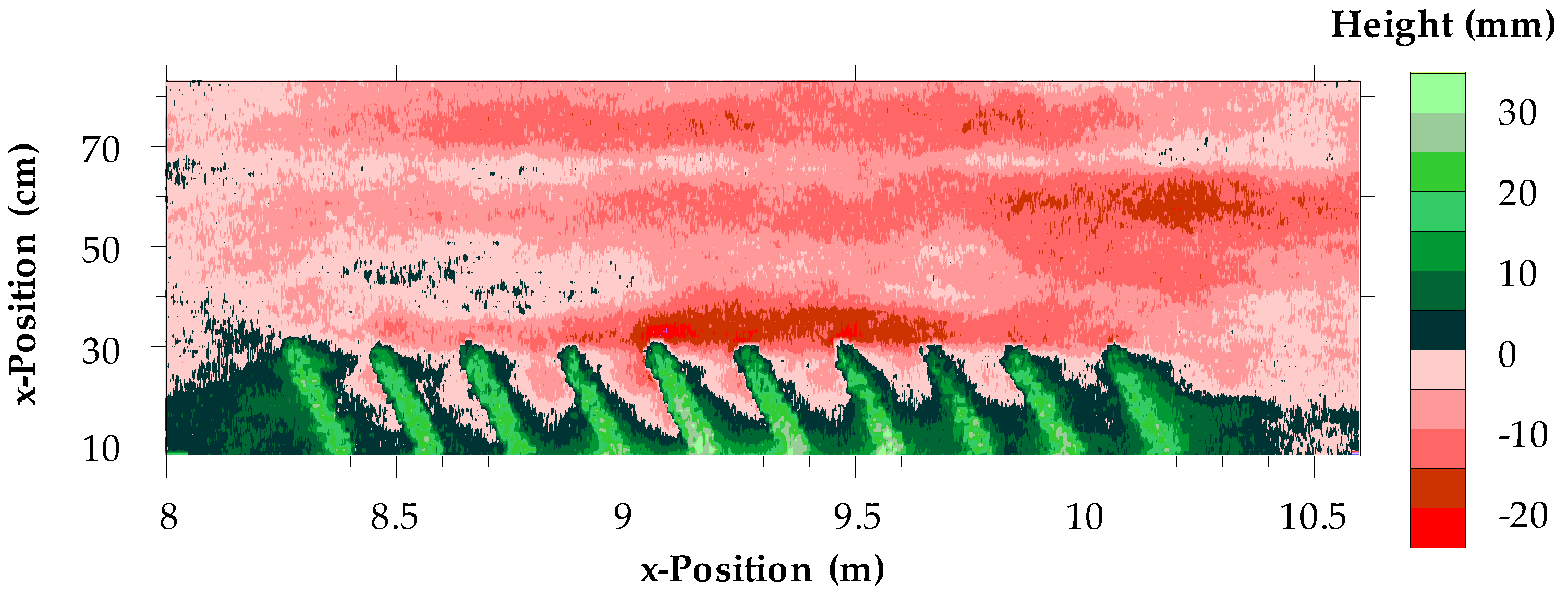
The effect of a groyne field made of gravel groynes on the bed morphology and the resulting backwater height was tested for a setup comparable to the run of GF 1 with dG = 12.5 cm and hN = 10 cm with respect to the aspect ratio dG/lP and the groyne field length (Table 1). Considering the roughness density, the setup was comparable to GF 1 with dG = 20 cm. The hydraulic conditions led to incipient motion. Sediment transported from upstream towards the groyne field was deposited in the groyne field, while the bed in the unblocked area eroded. The erosive forces became stronger along the groyne field, resulting in scouring at the groyne heads in the middle of the field as well as at the downstream end of the field towards the middle of the flume (Figure 7). The cross-sectionally averaged backwater height at the beginning of the groyne field was Δh = 0.57 cm, while for the two comparable experiments with fixed bed, the water level was increased by 1.45 cm and 1.9 cm, respectively (Figure 4). Although the blockage effect was even larger due to sediment deposition upstream of and within the groyne field, the roughness of the system was compensated distinctly by the areal erosion of the river bed. The resulting water level only increased by approximately 40% and 30%, respectively, compared to the backwater height of the fixed bed experiments. The reduced roughness of the mobile bed system is reflected by the considerably lower friction factor (Figure 6).
4. Conclusions
The hydraulic roughness of submerged groyne fields was investigated for two groyne types: varying groyne distances as well as varying and constant field lengths. For each test geometry, three hydraulic conditions were employed with relative submergences of 2, 4, and 6. The experiments were conducted in a straight flume with a fixed rough bed. One setup was conducted in a flume with a mobile gravel bed at hydraulic conditions for incipient motion to consider the influence of morphological changes on the roughness of the system.
For all setups, the absolute value of the backwater increased with increasing submergence. However, the relative backwater height decreased, confirming the applicability of submerged groynes for situations with restricted flood water levels. The relation between relative water level increase and groyne distance depended on the variability of the groyne field length. With increasing groyne distance and groyne field length (GF 1), the backwater approached a constant height, while for a constant groyne field length (GF 2), the backwater height reached a maximum at a certain groyne distance and decreased with further increasing distance. The different relationships were related to the combined contributions of the groyne density and the groyne field length to the total roughness. Thus, it is important to consider the resulting total length of a groyne field, besides the number and spacing of the groynes, when deriving a formula for calculating the flow resistance of a groyne field. This study investigated only one, quite short groyne field of constant length. Further tests are required to determine for which length the observed effect vanishes.
The change from a steep to an asymptotic increase (GF 1) and the maximum (GF 2), respectively, were found for the groyne distance where the inclined groynes did not overlap anymore. The distance between the head of the next downstream groyne and the toe of the upstream groyne was large enough that the overtopping flow could develop and interact with the flow in the unblocked area, like it is described in [14,15,22]. With increasing distance between the groynes, the losses due to this interaction decreased.
Analysis of the friction factor of a groyne field demonstrated the applicability of the concept of quasi smooth, wake interference and isolated roughness flow, which was developed for uniformly distributed bed roughness, to describe the total roughness of a groyne field. Thus, the comprehensive knowledge of rough bed flow can be used for studying the flow of submerged groyne fields.
These findings were independent of the type of groyne. The simplified shape of the multiplex groyne, especially the sharp edges, resulted in distinctly higher backwater effects compared to the gravel groyne with an irregular surface. It can be assumed, that this effect will affect the results of other studies with substitutes, e.g., plates instead of groyne models. While this can be considered as positive for backwater effects as the results are on the safe side, the results of the morphodynamic studies may lead to misinterpretations. The contribution of the adapted bed topography to the roughness of a river section with groynes resulted in a backwater, which was only approximately one-third of the corresponding backwater measured for fixed bed conditions. The study shows that care must be taken when simplifying the boundary conditions for laboratory experiments, regarding the investigated structure as well as the mobility of the bed, because not only can the magnitude of a measured parameter be affected, but also the functional relationships.
Author Contributions
Conceptualization, R.M. and K.K.; methodology, R.M.; validation, R.M., K.K.; formal analysis, R.M.; investigation, R.M.; resources, K.K.; data curation, R.M.; writing—original draft preparation, R.M.; writing—review and editing, K.K.; visualization, R.M.; supervision, K.K.; project administration, K.K.
Funding
This research received no external funding.
Acknowledgments
Many thanks are given to the students that were involved in the preparation and conduct of the experiments.
Conflicts of Interest
The authors declare no conflict of interest.
References
- Radspinner, R.R.; Diplas, P.; Lightbody, A.F.; Sotiropoulos, F. River training and ecological enhancement potential using in-stream structures. J. Hydraul. Eng. 2010, 136, 967–980. [Google Scholar] [CrossRef]
- Zaid, B.A. Development of Design Guidelines for Shallow Groynes. Ph.D. Thesis, TU Braunschweig, Braunschweig, Germany, 2017. [Google Scholar] [CrossRef]
- Shields, F.D., Jr.; Knight, S.S.; Cooper, C.M. Warmwater stream bank protection and fish habitat: A comparative study. Environ. Manag. 2000, 26, 317–328. [Google Scholar] [CrossRef]
- Bressan, F.; Papanicolaou, T. Scour around a variably submerged barb in a gravel bed stream. In Proceedings of the International Conference on Fluvial Hydraulics, RiverFlow, San José, Costa Rica, 5–7 September; Munoz, R.E.M., Ed.; Taylor & Francis Group: London, UK, 2012; pp. 333–339, ISBN 978-0-415-62129-8. [Google Scholar]
- Fang, D.; Sui, J.; Thring, R.W.; Zhang, H. Impacts of dimension and slope of submerged spur dikes on local scour processes-an experimental study. Int. J. Sediment Res. 2006, 21, 89–100. [Google Scholar]
- Hemmati, M.; Daraby, P. Erosion and sedimentation patterns associated with restoration structures of bendway weirs. J. Hydro-Environ. Res. 2019, 22, 19–28. [Google Scholar] [CrossRef]
- Jamieson, E.C.; Rennie, C.D.; Townsend, R.D. 3D flow and sediment dynamics in a laboratory channel bend with and without stream barbs. J. Hydraul. Eng. 2013, 139, 154–166. [Google Scholar] [CrossRef]
- Kadota, A.; Muraoka, H.; Suzuki, K. River-Bed Configuration Formed by a Permeable Groyne of Stone Gabion. In Proceedings of the International Conference on Fluvial Hydraulics, RiverFlow, Çeşme, Turkey, 3–5 September 2008; Altinakar, M.S., Kokpinar, M.A., Aydin, I., Cokgor, S., Kirkgoz, S., Eds.; Kubaba: Ankara, Turkey, 2008; pp. 1531–1540, ISBN 978-605-60136-1-4. [Google Scholar]
- Kuhnle, R.A.; Alonso, C.V.; Shields, F.D., Jr. Local scour associated with angled spur dikes. J. Hydraul. Eng. 2002, 128, 1087–1093. [Google Scholar] [CrossRef]
- M#xF6;, R.; Koll, K. Influence of a single submerged groyne on the bed morphology and the flow field. In Proceedings of the International Conference on Fluvial Hydraulics, RiverFlow 2014. Lausanne, Switzerland, 3–5 September 2014; Schleiss, A.J., de Cesare, G., Franca, M.J., Pfister, M., Eds.; Taylor & Francis Group: London, UK, 2014; pp. 1447–1454, ISBN 978-1-138-02674-2. [Google Scholar]
- Julien, P.Y.; Duncan, J.R. Optimal Design Criteria of Bendway Weirs from Numerical Simulations and Physical Model Studies; Technical Paper; Colorado State University: Fort Collins, CO, USA, 2003. [Google Scholar]
- Kuhnle, R.A.; Jia, Y.; Alonso, C.V. Measured and simulated flow near a submerged spur dike. J. Hydraul. Eng. 2008, 134, 916–924. [Google Scholar] [CrossRef]
- Mende, M. Naturnaher Uferschutz mit Lenkbuhnen-Grundlagen, Analytik und Bemessung. Ph.D. Thesis, TU Braunschweig, Braunschweig, Germany, 2014. [Google Scholar]
- Sukhodolov, A.N. Hydrodynamics of groyne fields in a straight river reach: Insight from field experiments. J. Hydraul. Res. 2014, 52, 105–120. [Google Scholar] [CrossRef]
- Uijtewaal, W.S.J. Effects of groyne layout on the flow in groyne fields: Laboratory Experiments. J. Hydraul. Eng. 2005, 131, 782–791. [Google Scholar] [CrossRef]
- Lagasse, P.F.; Clopper, P.E.; Pag#xE1;, J.E.; Zevenbergen, L.W.; Arneson, L.A.; Schall, J.D.; Girard, L.G. Bridge Scour and Stream Instability Countermeasures-Experience, Selection and Design Guidance, 3rd ed.; HEC-23; US Dept. of Transportation: Fort Collins, CO, USA, 2009; Volume 2.
- USDA. Technical Note 23 Design of Stream Barbs-Version 2.0; Engineering Technical Note No. 23; United States Department of Agriculture, Natural Resources Conservation Service: Portland, OR, USA, 2005.
- USACE. Physical Model Test for Bendway Weir Design Criteria; Report No. ERDC/CHL TR-02-28; U.S. Army Corps of Engineers: Vicksburg, MS, USA, 2002. [Google Scholar]
- Yossef, M.F.M. Morphodynamics of Rivers with Groynes; Delft University Press: Delft, The Netherlands, 2005; p. 240. [Google Scholar]
- Azinfar, H.; Kells, J.A. Drag force and associated backwater effect due to an open channel spur dike field. J. Hydraul. Res. 2011, 49, 248–256. [Google Scholar] [CrossRef]
- Morris, H.M. Flow in rough conduits. Trans. ASCE 1955, 120, 373–410. [Google Scholar]
- Chow, V.T. OPEN-Channel Hydraulics; McGraw-Hill Inc.: New York, NY, USA, 1959. [Google Scholar]
- Dittrich, A.; Koll, K. Velocity field and resistance of flow over rough surfaces with large and small relative submergence. Int. J. Sediment Res. 1997, 3, 21–33. [Google Scholar]
- Dittrich, A. Wechselwirkung Morphologie/Strömung Naturnaher Fließgewässer; Habilitation at Universität Karlsruhe (TH): Karlsruhe, Germany, 1998. [Google Scholar]
- Canovaro, F.; Paris, E.; Solari, L. Effects of macro-scale bed roughness geometry on flow resistance. Water Resour. Res. 2007, 43, 1–17. [Google Scholar] [CrossRef]
- Zaid, B.A.; Koll, K. Sensitivity of the flow to the inclination of a single submerged groyne in a curved flume. In Hydrodynamic and Mass Transport at Freshwater Aquatic Interfaces; GeoPlanet: Earth and Planetary Sciences; Rowiń, P.M., Marion, A., Eds.; Springer: Heidelberg, Germany, 2016; pp. 245–254. [Google Scholar] [CrossRef]
- Zaid, B.A.; Koll, K. Experimental investigation of the location of a submerged groyne for bank protection. In Proceedings of the International Conference on Fluvial Hydraulics, RiverFlow 2016, Saint Louis, MO, USA, 11–14 July 2016; Constantinescu, G., Garcia, M., Hanes, D., Eds.; Taylor & Francis Group: London, UK, 2016; pp. 1286–1292, ISBN 978-1-138-02913-2. [Google Scholar] [CrossRef]
Figure 1.
Top view on (a) the multiplex groyne model and (b) the gravel groyne model.

Figure 2.
Example of a groyne field setup section with groyne dimension parameters. The white dots exemplarily indicate positions of water level measurements and the square shows the related ground Area (A) of a single groyne.
Figure 2.
Example of a groyne field setup section with groyne dimension parameters. The white dots exemplarily indicate positions of water level measurements and the square shows the related ground Area (A) of a single groyne.

Figure 3.
Water level change (Δh) along the main flow direction (groyne field from x = 7 m to 8.5 m) for gravel groynes with distance dG = 15 cm (GF 2).
Figure 3.
Water level change (Δh) along the main flow direction (groyne field from x = 7 m to 8.5 m) for gravel groynes with distance dG = 15 cm (GF 2).

Figure 4.
Relative increase of the water depth at x = 6.9 m as a function of the distance between groynes dG and approach flow in series GF 1 (open symbols = multiplex groynes; filled symbols = gravel groynes).
Figure 4.
Relative increase of the water depth at x = 6.9 m as a function of the distance between groynes dG and approach flow in series GF 1 (open symbols = multiplex groynes; filled symbols = gravel groynes).

Figure 5.
Relative increase of the water depth at x = 6.9 m as a function of the distance between groynes dG and approach flow for gravel groynes with varying field length (GF 1: filled symbols) and constant field length (GF 2: shaded symbols).
Figure 5.
Relative increase of the water depth at x = 6.9 m as a function of the distance between groynes dG and approach flow for gravel groynes with varying field length (GF 1: filled symbols) and constant field length (GF 2: shaded symbols).

Figure 6.
Friction coefficient f of the groyne fields as a function of groyne distance dG and roughness density ck, resp. (open symbols = multiplex groynes in series GF 1; filled symbols = gravel groynes in series GF 1; shaded symbols = gravel groynes in series GF 2; green dot: GF 3).
Figure 6.
Friction coefficient f of the groyne fields as a function of groyne distance dG and roughness density ck, resp. (open symbols = multiplex groynes in series GF 1; filled symbols = gravel groynes in series GF 1; shaded symbols = gravel groynes in series GF 2; green dot: GF 3).

Figure 7.
Bed topography at the end of the mobile bed experiment (flow direction from left to right).
Figure 7.
Bed topography at the end of the mobile bed experiment (flow direction from left to right).


Table 1.
Experimental parameters.
| Series | Groyne Type | m (-) | dG (cm) | dG/lP (-) | lGF (m) | ck (-) | hN (cm) | Fr (-) | Q (L/s) |
|---|---|---|---|---|---|---|---|---|---|
| GF 1 | MultiplexGravel | 15 | 10 | 0.5 | 1.4 | 0.25 | 5, 10, 15 | 0.59, 0.65, 0.66 | 11.6, 35.7, 69.7 |
| 12.5 | 0.625 | 1.75 | 0.2 | ||||||
| 15* | 0.75 | 2.1* | 0.17* | ||||||
| 20 | 1 | 2.8 | 0.125 | ||||||
| 25 | 1.25 | 3.5 | 0.1 | ||||||
| 35 | 1.75 | 4.9 | 0.07 | ||||||
| 60** | 3 | 7.8** | 0.04** | ||||||
| GF 2 | Gravel | 16 | 10 | 0.5 | 1.5 | 0.25 | 5, 10, 15 | 0.59, 0.65, 0.66 | 11.6, 35.7, 69.7 |
| 11 | 15 | 0.75 | 0.17 | ||||||
| 6 | 30 | 1.5 | 0.083 | ||||||
| 4 | 50 | 2.5 | 0.05 | ||||||
| GF 3 | Gravel | 10 | 20 | 0.645 | 1.8 | 0.125 | 10 | 0.59 | 58.6 |
* only multiplex groynes, ** only 14 groynes.
© 2019 by the authors. Licensee MDPI, Basel, Switzerland. This article is an open access article distributed under the terms and conditions of the Creative Commons Attribution (CC BY) license (http://creativecommons.org/licenses/by/4.0/).
Share and Cite
MDPI and ACS Style
Möws, R.; Koll, K. Roughness Effect of Submerged Groyne Fields with Varying Length, Groyne Distance, and Groyne Types. Water 2019, 11, 1253. https://doi.org/10.3390/w11061253
AMA Style
Möws R, Koll K. Roughness Effect of Submerged Groyne Fields with Varying Length, Groyne Distance, and Groyne Types. Water. 2019; 11(6):1253. https://doi.org/10.3390/w11061253
Chicago/Turabian StyleMöws, Ronald, and Katinka Koll. 2019. "Roughness Effect of Submerged Groyne Fields with Varying Length, Groyne Distance, and Groyne Types" Water 11, no. 6: 1253. https://doi.org/10.3390/w11061253
Note that from the first issue of 2016, this journal uses article numbers instead of page numbers. See further details here.