Rural Households’ Willingness to Accept Compensation Standards for Controlling Agricultural Non-Point Source Pollution: A Case Study of the Qinba Water Source Area in Northwest China

Abstract
:1. Introduction
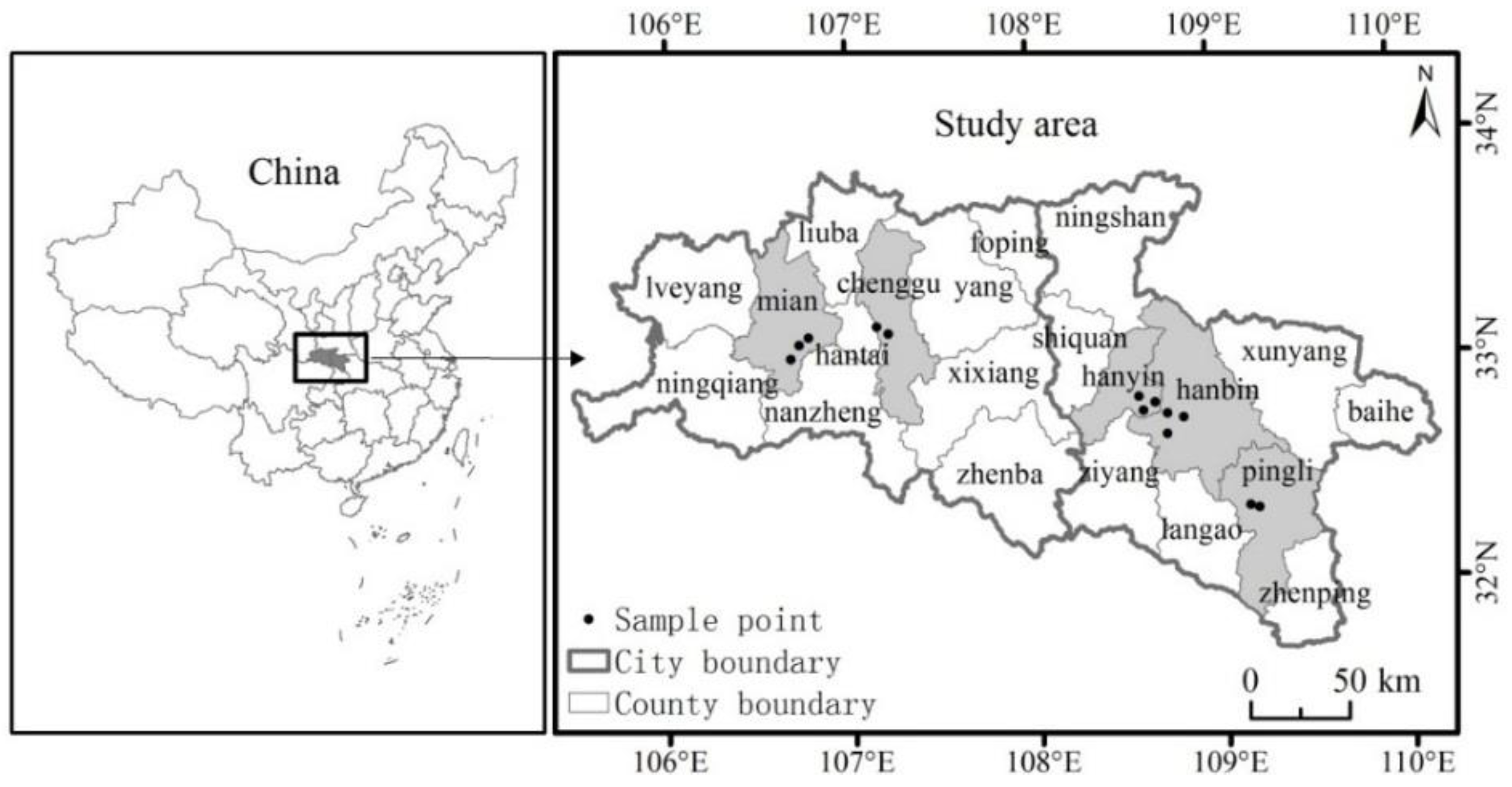
2. Study Area
3. Methodology
3.1. Choice Experiment Design
3.2. RPL Model
3.3. Bias Handling
3.4. Data
4. Results and Analysis
4.1. Multicollinearity Test of Socio-Economic Variables of Rural Households
4.2. Influencing Factors of Rural Households’ Willingness to Accept Compensation
4.3. Compensation Standard Calculation
4.4. Reasonableness Test of Compensation Standard
5. Conclusions and Discussion
5.1. Discussion
5.2. Conclusions and Policy Implication
Author Contributions
Funding
Acknowledgments
Conflicts of Interest
References
- Panagopoulos, Y.; Makropoulos, C.; Mimikou, M. Reducing surface water pollution through the assessment of the cost-effectiveness of BMPs at different spatial scales. J. Environ. Manag. 2011, 92, 2823–2835. [Google Scholar] [CrossRef] [PubMed]
- Jabbar, F.K.; Grote, K. Statistical assessment of nonpoint source pollution in agricultural watersheds in the Lower Grand River watershed, MO, USA. Environ. Pollut. Res. 2019, 26, 1487–1506. [Google Scholar] [CrossRef] [PubMed]
- Jin, S.Q.; Wu, Y. Is agricultural non-point source pollution the primary cause of water pollution? Test Based on the Data of Huaihe River. Chin. Rural Econ. 2014, 9, 71–81. [Google Scholar]
- Junakova, N.; Balintova, M.; Vodicka, R.; Junak, J. Prediction of Reservoir Sediment Quality Based on Erosion Processes in Watershed Using Mathematical Modelling. Environments 2018, 5, 6. [Google Scholar] [CrossRef]
- Carpenter, S.R.; Caraco, N.F.; Correll, D.L.; Howarth, R.W.; Sharpley, A.N.; Smith, V.H. Nonpoint pollution of surface waters with phosphorus and nitrogen. Ecol. Appl. 1998, 8, 559–568. [Google Scholar] [CrossRef]
- Halliday, S.J.; Skeffington, R.A.; Bowes, M.J.; Gozzard, E.; Newman, J.R.; Loewenthal, M.; Palmer-Felgate, E.J.; Jarvie, H.P.; Wade, A.J. The Water quality of the River Enborne, UK: Observations from high-frequency monitoring in a rural, lowland river system. Water 2014, 6, 150–180. [Google Scholar] [CrossRef]
- Power, M.E.; Brozovic, N.; Bode, C.; Zilberman, D. Spatially Explicit Tools for Understanding and Sustaining Inland Water Ecosystems. Front. Ecol. Environ. 2005, 3, 47–55. [Google Scholar] [CrossRef]
- Ge, Y.X.; Liang, L.J.; Jie, Y.M. Study on the Construction and Operation of Ecological Compensation Mechanism for Water Source. Issues Agric. Econ. 2006, 9, 22–28. [Google Scholar]
- Hu, H.Y.; Huang, G.R. Monitoring of Non-Point Source Pollutions from an Agriculture Watershed in South China. Water 2014, 6, 3828–3840. [Google Scholar] [CrossRef] [Green Version]
- Psaltopoulos, D.; Wade, A.J.; Skuras, D.; Kernan, M.; Tyllianakis, E.; Erlandsson, M. False positive and false negative errors in the design and implementation of agri-environmental policies: A case study on water quality and agricultural nutrients. Sci. Total Environ. 2017, 575, 1087–1099. [Google Scholar] [CrossRef] [Green Version]
- Vergano, L.; Nunes, P.A.L.D. Analysis and evaluation of ecosystem resilience: An economic perspective with an application to the Venice lagoon. Biodivers. Conserv. 2007, 16, 3385–3408. [Google Scholar] [CrossRef]
- Engel, S.; Pagiola, S.; Wunder, S. Designing payments for environmental services in theory and practice: An overview of the issues. Ecol. Econ. 2008, 65, 663–674. [Google Scholar] [CrossRef]
- Wu, Z.N.; Guo, X.; Lv, C.M.; Wang, H.L.; Di, D.Y. Study on the quantification method of water pollution ecological compensation standard based on emergy theory. Ecol. Indic. 2017, 92, 189–194. [Google Scholar] [CrossRef]
- Nesha, B.B.; James, C.R.S.; Mette, T.; Klaus, H. Evaluating farmers’ likely participation in a payment programme for water quality protection in the UK uplands. Reg. Environ. Chang. 2013, 13, 633–647. [Google Scholar]
- Liu, M.C.; Xiong, Y.; Yuan, Z.; Min, Q.W.; Sun, Y.H.; Fuller, A.M. Standards of ecological compensation for traditional eco-agriculture: Taking rice-fish system in Hani terrace as an example. J. Mt. Sci. 2014, 11, 1049–1059. [Google Scholar] [CrossRef]
- Claassen, R.; Cattaneo, A.; Johansson, R. Cost-effective design of agri-environmental payment programs: U.S. experience in theory and practice. Ecol. Econ. 2008, 65, 737–752. [Google Scholar] [CrossRef]
- Costanza, R.; Ralph, A.; Rudolf, D.G.; Stephen, F.; Monica, G.; Bruce, H.; Karin, L.; Shahid, N.; Robert, V.; Jose, P.; et al. The value of the world’s ecosystem services and natural capital. Nature 1997, 15, 253–260. [Google Scholar] [CrossRef]
- Sheng, W.P.; Zhen, L.; Xie, G.D.; Xiao, Y. Determining eco-compensation standards based on the ecosystem services value of the mountain ecological forests in Beijing, China. Ecosyst. Serv. 2017, 26, 422–430. [Google Scholar] [CrossRef]
- Zhou, C.; Ding, X.D.; Li, G.P.; Wang, H.Z. Ecological compensation standards in the water source area of the middle route project of the South-North water transfer project. Resour. Sci. 2015, 37, 792–804. [Google Scholar]
- Gao, Z.B.; Wang, X.L.; Su, J.; Chen, Z.F.; Zheng, M.X.; Sun, Y.Y.; Ji, D.F. Ecological Compensation of Dongjiang River Basin Based on Evaluation of Ecosystem Service Value. J. Ecol. Rural Environ. 2018, 34, 563–570. [Google Scholar]
- Fan, M.; Chen, L. Spatial characteristics of land uses and ecological compensations based on payment for ecosystem services model from 2000 to 2015 in Sichuan Province, China. Ecol. Inform. 2019, 50, 162–183. [Google Scholar] [CrossRef]
- Knoke, T.; Hildebrandt, P.; Klein, D.; Mujica, R.; Moog, M.; Mosandl, R. Financial compensation and uncertainty: Using mean-variance rule and stochastic dominance to derive conservation payments for secondary forests. Can. J. For. Res. 2008, 38, 3033–3046. [Google Scholar] [CrossRef]
- Mashayekhi, Z.; Danehkar, A.; Sharzehi, G.A.; Majed, V. Coastal Communities WTA Compensation for conservation of mangrove forests: A choice experiment approach. Knowl. Manag. Aquat. Ecosyst. 2016, 417, 1–10. [Google Scholar] [CrossRef]
- Moss, L.R. Local governments reduce costs through pollution prevention. J. Clean. Prod. 2008, 16, 704–708. [Google Scholar] [CrossRef]
- Lescot, J.M.; Bordenave, P.; Petit, K.; Leccia, O. A spatially-distributed cost-effectiveness analysis framework for controlling water pollution. Environ. Model. Softw. 2013, 41, 107–122. [Google Scholar] [CrossRef]
- Bovenberg, A.L.; Goulder, L.H.; Jacobsen, M.R. Costs of alternative environmental policy instruments in the presence of industry compensation requirements. J. Public Econ. 2008, 92, 1236–1253. [Google Scholar] [CrossRef] [Green Version]
- Kopp, R.J.; Krupnick, A. Agricultural Policy and the Benefits of Ozone Control. Am. J. Agric. Econ. 1987, 69, 956–962. [Google Scholar] [CrossRef]
- Geng, X.Y.; Ge, Y.X.; Zhang, H.N. Study on ecological compensation standard of watershed based on reset cost. China Popul. Resour. Environ. 2018, 28, 140–147. [Google Scholar]
- He, K.; Zhang, J.B.; Zeng, Y.M.; Zhang, L. Households’ willingness to accept compensation for agricultural waste recycling: Taking biogas production from livestock manure waste in Hubei, P.R. China as an example. J. Clean. Prod. 2016, 131, 410–420. [Google Scholar] [CrossRef]
- Mutandwa, E.; Grala, R.K.; Petrolia, D.R. Estimates of willingness to accept compensation to manage pine stands for ecosystem services. For. Policy Econ. 2019, 102, 75–85. [Google Scholar] [CrossRef]
- Shaanxi Statistical Bureau. Shaanxi Statistical Yearbook 2017; China Statistics Publishing House: Beijing, China, 2018.
- Zhu, Y.Y.; Liu, Y.; Zhou, B.H.; Jiang, Q.F.; Wu, D.W. The temporal and spatial distribution of nitrogen in Danjiangkou Reservoir Watershed. Environ. Monit. China 2016, 32, 50–57. [Google Scholar]
- Zhu, Y.Y.; Tian, J.J.; Li, H.L.; Jiang, Q.F.; Liu, Y. Water qaulity assessment and pollution profile identification of Danjiangkou Reservoir, China. J. Agro-Environ. Sci. 2016, 35, 139–147. [Google Scholar]
- Zhao, Z.P.; Yan, S.; Tong, Y.A. Eco-environmental status assessment and treatment measure in the upper Hanjing River Basin. Bull. Soil Water Conserv. 2012, 32, 32–36. [Google Scholar]
- Urama, K.C.; Hodge, I.D. Are stated preferences convergent with revealed preferences? Empirical evidence from Nigeria. Ecol. Econ. 2006, 59, 24–37. [Google Scholar] [CrossRef]
- Guignet, D. The impacts of pollution and exposure pathways on home values: A stated preference analysis. Ecol. Econ. 2012, 82, 53–63. [Google Scholar] [CrossRef]
- Yao, L.Y.; Deng, J.F.; Johnston, R.J.; Khan, I.; Zhao, M.J. Evaluating willingness to pay for the temporal distribution of different air quality improvements: Is China’s clean air target adequate to ensure welfare maximization? Can. J. Agric. Econ./Rrevue Can. D’Agroecon. 2018, 67, 215–232. [Google Scholar] [CrossRef]
- Schultz, E.T.; Johnston, R.J.; Segerson, K.; Besedin, E.Y. Integrating Ecology and Economics for Restoration: Using Ecological Indicators in Valuation of Ecosystem Services. Restor. Ecol. 2012, 20, 304–310. [Google Scholar] [CrossRef] [Green Version]
- Garcia, J.H.; Cherry, T.L.; Kallbekken, S.; Torvanger, A. Willingness to accept local wind energy development: Does the compensation mechanism matter? Energy Policy 2016, 199, 165–173. [Google Scholar] [CrossRef]
- Bateman, I.J.; Day, B.H.; Jones, A.P.; Jude, S. Reducing gain–loss asymmetry: A virtual reality choice experiment valuing land use change. J. Environ. Econ. Manag. 2009, 58, 106–118. [Google Scholar] [CrossRef]
- Rolfe, J.; Bennett, J. The impact of offering two versus three alternatives in choice modelling experiments. Ecol. Econ. 2009, 68, 1140–1148. [Google Scholar] [CrossRef]
- Yao, L.Y.; Zhao, M.J.; Cai, Y.; Yin, Z.W. Public Preferences for the Design of a Farmland Retirement Project: Using Choice Experiments in Urban and Rural Areas of Wuwei, China. Sustainability 2018, 10, 1579. [Google Scholar] [CrossRef]
- Zhao, M.J.; Johnston, R.J.; Schultz, E.T. What to value and how? Ecological indicator choices in stated preference valuation. Environ. Resour. Econ. 2013, 56, 3–25. [Google Scholar] [CrossRef]
- Briassoulis, D.; Hiskakis, M.; Babou, E.; Antiohos, S.K.; Papadi, C. Experimental investigation of the quality characteristics of agricultural plastic wastes regarding their recycling and energy recovery potential. Waste Manag. 2012, 32, 1075–1090. [Google Scholar] [CrossRef] [PubMed]
- Sims, J.T.; Goggin, N.; Mcdermott, J. Nutrient management for water quality protection: Integrating research into environmental policy. Water Sci. Technol. 1999, 39, 291–298. [Google Scholar] [CrossRef]
- Ministry of Agriculture of the People’s Republic of China. Action Plan for the Zero Increase of Fertilizer Use in 2020 [EB/OL]. (2017–2003–07) [2015–2003–18]. Available online: http://jiuban.moa.gov.cn/zwllm/tzgg/tz/201503/t20150318_4444765. htm (accessed on 1 April 2019).
- Dahshan, H.; Megahed, A.M.; Abdelall, A.M.; Abdelkader, M.A.; Nabaw, E.; Elbana, M.H. Monitoring of pesticides water pollution-The Egyptian River Nile. Iran. J. Environ. Health Sci. Eng. 2016, 14, 1–15. [Google Scholar] [CrossRef] [PubMed]
- Zhu, D.; Kong, X.; Gu, J.P. Irrational Equilibrium of Overuse of Pesticides by Farmers: Evidence from Farmers in Southern Jiangsu. Chin. Rural Econ. 2014, 8, 17–29. [Google Scholar]
- Mcfadden, D. Conditional logit analysis of qualitative choice behavior. In Frontiers in Econometrics; Zarembka, P., Ed.; Academic Press: New York, NY, USA; pp. 105–142.
- Xu, T.; Zhao, M.J.; Qiao, D.; Yao, L.Y.; Yan, Y. Subsidy policy design of two oriented technology based on farmer households’ preference. J. Northwest A&F Univ. (Soc. Sci. Ed.) 2018, 18, 109–118. [Google Scholar]
- Quan, S.W. Advances in Selective Experimental Methods. Econ. Inf. 2016, 1, 127–141. [Google Scholar]
- Riccarda, M.; Roberta, R.; Sandra, N. Testing hypothetical bias with a real choice experiment using respondents’ own money. Eur. Rev. Agric. Econ. 2014, 41, 25–46. [Google Scholar]
- Train, K.; Wilson, W.W. Estimation on stated-preference experiments constructed from revealed-preference choices. Transp. Res. Part B Methodol. 2008, 42, 191–203. [Google Scholar] [CrossRef]
- Brown, T.C.; Ajzen, I.; Hrubes, D. Further tests of entreaties to avoid hypothetical bias in referendum contingent valuation. J. Environ. Econ. Manag. 2003, 46, 353–361. [Google Scholar] [CrossRef] [Green Version]
- List, J.A. Do explicit warnings eliminate the hypothetical bias in elicitation procedures? Evidence from field auctions for sportscards. Am. Econ. Rev. 2001, 91, 1498–1507. [Google Scholar] [CrossRef]
- Silva, A.; Nayga, R.M.; Campbell, B.L.; Park, J.L. Can perceived task complexity influence cheap talk’s effectiveness in reducing hypothetical bias in stated choice studies? Appl. Econ. Lett. 2012, 19, 1711–1714. [Google Scholar] [CrossRef]
- Li, J.G.; Gao, Y.M.; Zang, J.M. The impact of farmers’ risk awareness on land transfer decision making behavior. J. Agrotech. 2014, 11, 21–30. [Google Scholar]
- Liang, F.; Zhu, Y.C. Analysis of farmer’s vulnerability to poverty from the perspective of resource endowment. J. Northwest A&F Univ. (Soc. Sci. Ed.) 2018, 18, 131–140. [Google Scholar]
- Romy, G. Motivations and attitudes influence farmers’ willingness to participate in biodiversity conservation contracts. Agric. Syst. 2015, 137, 154–165. [Google Scholar]
- Hole, A.R. Fitting mixed logit models by using maximum simulated likelihood. Stata J. 2007, 7, 388–401. [Google Scholar] [CrossRef]
- Cai, J. Pesticide Packaging waste recycling: Support attitude and model choice. Res. Econ. Manag. 2013, 12, 67–74. [Google Scholar]
- Kristrom, B.; Riera, P. Is the income elasticity of environmental improvements less than one. Environ. Resour. Econ. 1996, 7, 45–55. [Google Scholar] [CrossRef]
- Tyllianakis, E.; Skuras, D. The income elasticity of Willingness-To-Pay (WTP) revisited: A meta-analysis of studies for restoring Good Ecological Status (GES) of water bodies under the Water Framework Directive (WFD). J. Environ. Manag. 2016, 182, 531–541. [Google Scholar] [CrossRef]


| Attribute | Selection 1 | Selection 2 | Selection 3 |
|---|---|---|---|
| Fertilizer reduction | Reducing by 1/4 | Reducing by 1/2 | No reduction of fertilizer and pesticides, part recovery of agricultural waste |
| Pesticide reduction | Reducing by 1/2 | No reduction | |
| Agricultural waste recovery rate | No reduction | All classified recovery | |
| Compensation (¥/(year·mu)) | ¥200 | ¥500 | ¥0 |
| Please choice | □ | □ | □ |
| Indicator | Definitions and Assignments | Mean | Standard Deviation |
|---|---|---|---|
| Age | Age of rural households surveyed | 57.13 | 110.27 |
| Education attained | Years of schooling | 6.36 | 12.94 |
| Number of labor forces | Number of labor forces in rural households | 2.95 | 1.80 |
| Households’ income | [0, $3011) = 1; [$3011, $6022) = 2; [$6022, $9033) = 3; [$9033, $12,044) = 4; [$12,044, $15,055) = 5; [$15,055,+∞) = 6 | 3.12 | 3.08 |
| Cultivated land | Cultivated land of rural households | 4.23 | 19.85 |
| Ecological benefit perception | ANSP control has ecological benefits: total disapproval = 1; disapproval = 2; general = 3; comparative approval = 4; total approval = 5 | 3.99 | 1.21 |
| Government policy perception | I understand NASP control policy: total disapproval = 1; disapproval = 2; general = 3; comparative approval = 4; total approval = 5 | 2.36 | 1.59 |
| Dependent Variables | Independent Variables | Collinearity Statistics | |
|---|---|---|---|
| Tolerance | VIF | ||
| Age | Number of labor forces | 0.93 | 1.08 |
| Ecological benefit Perception | 0.95 | 1.05 | |
| rural household income | 0.95 | 1.05 | |
| Government policy perception | 0.97 | 1.04 | |
| Education attained | 0.97 | 1.04 | |
| Cultivated land | 0.99 | 1.02 | |
| Mean VIF | 1.05 | ||
| Indicator | Model 1 | Model2 | ||||
|---|---|---|---|---|---|---|
| Mean | Std. Error | Std. Dev. | Mean | Std. Error | Std. Dev. | |
| ASC | −29.009 *** | 9.081 | −24.786 *** | −19.875 ** | 8.706 | 27.042 *** |
| Compensation | 0.004 *** | 0.000 | - | 0.004 *** | 0.000 | - |
| Fertilizer reduction | −0.006 ** | 0.002 | 0.006 | −0.006 *** | 0.002 | −0.007 |
| Pesticide reduction | −0.004 ** | 0.002 | −0.009 * | −0.004 ** | 0.002 | 0.013 *** |
| Agricultural waste recovery rate | 0.090 | 0.084 | 0.593 ** | 0.111 | 0.095 | 0.943 *** |
| ASC × Age | 0.275 ** | 0.123 | 0.509 *** | |||
| ASC × Education attained | −0.250 | 0.205 | 0.097 | |||
| ASC × Number of labor forces | −0.579 | 0.504 | −3.012 *** | |||
| ASC × Rural household income | −0.706 ** | 0.336 | 1.805 *** | |||
| ASC × Cultivated land | 0.028 | 0.101 | −0.121 | |||
| ASC × Ecological benefit perception | −5.712 *** | 1.533 | -4.914 *** | |||
| ASC × Government policy perception | −11.184 *** | 2.909 | 0.481 | |||
| Log likelihood | −1354.814 | −790.34772 | ||||
| Prob > chi2 | 0.000 | 0.000 | ||||
| Attribute | Marginal Compensation Standard | Compensation of World Average | Compensation of Organic Production | |||
|---|---|---|---|---|---|---|
| Attribute Change | Compensation Standard ($/ha) | Attribute Change | Compensation Standard ($/ha) | Attribute Change | Compensation Standard ($/ha) | |
| Fertilizer reduction | Reducing by 1% | 3.40 | Reducing by 60% | 204.06 | Reducing by 100% | 340.09 |
| Pesticide reduction | Reducing by 1% | 2.00 | Reducing by 73% | 146.10 | Reducing by 100% | 200.14 |
| Total | 5.40 | 350.16 | 540.23 | |||
© 2019 by the authors. Licensee MDPI, Basel, Switzerland. This article is an open access article distributed under the terms and conditions of the Creative Commons Attribution (CC BY) license (http://creativecommons.org/licenses/by/4.0/).
Share and Cite
Li, X.; Liu, W.; Yan, Y.; Fan, G.; Zhao, M. Rural Households’ Willingness to Accept Compensation Standards for Controlling Agricultural Non-Point Source Pollution: A Case Study of the Qinba Water Source Area in Northwest China. Water 2019, 11, 1251. https://doi.org/10.3390/w11061251
Li X, Liu W, Yan Y, Fan G, Zhao M. Rural Households’ Willingness to Accept Compensation Standards for Controlling Agricultural Non-Point Source Pollution: A Case Study of the Qinba Water Source Area in Northwest China. Water. 2019; 11(6):1251. https://doi.org/10.3390/w11061251
Chicago/Turabian StyleLi, Xiaoping, Wenxin Liu, Yan Yan, Gongyuan Fan, and Minjuan Zhao. 2019. "Rural Households’ Willingness to Accept Compensation Standards for Controlling Agricultural Non-Point Source Pollution: A Case Study of the Qinba Water Source Area in Northwest China" Water 11, no. 6: 1251. https://doi.org/10.3390/w11061251