Non-Stationary Bayesian Modeling of Annual Maximum Floods in a Changing Environment and Implications for Flood Management in the Kabul River Basin, Pakistan

Abstract

Recent evidence of regional climate change associated with the intensification of human activities has led hydrologists to study a flood regime in a non-stationarity context. This study utilized a Bayesian framework with informed priors on shape parameter for a generalized extreme value (GEV) model for the estimation of design flood quantiles for “at site analysis” in a changing environment, and discussed its implications for flood management in the Kabul River basin (KRB), Pakistan. Initially, 29 study sites in the KRB were used to evaluate the annual maximum flood regime by applying the Mann–Kendall test. Stationary (without trend) and a non-stationary (with trend) Bayesian models for flood frequency estimation were used, and their results were compared using the corresponding flood frequency curves (FFCs), along with their uncertainty bounds. The results of trend analysis revealed significant positive trends for 27.6% of the gauges, and 10% showed significant negative trends at the significance level of 0.05. In addition to these, 6.9% of the gauges also represented significant positive trends at the significance level of 0.1, while the remaining stations displayed insignificant trends. The non-stationary Bayesian model was found to be reliable for study sites possessing a statistically significant trend at the significance level of 0.05, while the stationary Bayesian model overestimated or underestimated the flood hazard for these sites. Therefore, it is vital to consider the presence of non-stationarity for sustainable flood management under a changing environment in the KRB, which has a rich history of flooding. Furthermore, this study also states a regional shape parameter value of 0.26 for the KRB, which can be further used as an informed prior on shape parameter if the study site under consideration possesses the flood type “flash”. The synchronized appearance of a significant increase and decrease of trends within very close gauge stations is worth paying attention to. The present study, which considers non-stationarity in the flood regime, will provide a reference for hydrologists, water resource managers, planners, and decision makers.

1. Introduction

The comprehensive understanding of flood regimes is an important challenge in hydrology. Hydrologists and engineers customarily use flood frequency analysis (FFA) as a tool to understand flood regimes throughout the world. FFA estimates the flood peak for a given return period, but the currently used methods of FFA assume that the flood time series are independent and identically distributed [1,2,3] or, in other words, have no trends and unanticipated variations [4]. Indeed, the concept of stationarity was and is being adopted to design water resources infrastructure and flood protection works all around the globe. In recent decades, the climate system has been under stress due to natural variations in the global climate, and human activity also has a potential influence on regional climate that is ultimately intensifying the hydrologic cycle [5]. The hypothesis of stationarity has become widely questionable due to this regional and global change. Keeping this point of view, several studies have tried to explore the validity of this hypothesis in flood regimes in many regions around the world, considering the effect of natural climate variability [6,7,8,9,10,11,12] or land use changes [13,14,15]. The results of these studies have shown clear violations of the assumption of stationarity, which is consistent with studies that indicate an intensification of the hydrologic cycle [16,17].

Particularly, the KRB in the Hindu Kush Himalayan Range (HKH) is exposed to disturbances from the South Asian monsoon originating from the Bay of Bengal. Several recent studies represented a paucity of stationarity and indicated the intensification in some elements of the hydrologic cycle at the regional scale. The results of these studies investigated the change in the rainfall regime of the KRB. For instance, the number of consecutive wet days has been increasing significantly in the Peshawar valley, with a total change of 2.16 at a 95% confidence level. Consecutive wet days have also increased at Saidu Sharif in the Swat valley and Chitral [18]. Ahmad et al. [19] investigated trends in rainfall over the entire Swat River basin, a sub-basin of the KRB. They observed the highest positive trend (7.48 mm year⁻¹) at the Saidu Sharif in Swat valley. For annual precipitation time series, statistically insignificant trends were revealed for the whole Swat River basin. However, significant positive increasing trends of precipitation (2.18 mm year⁻¹) were observed in the Lower Swat basin. Saidu Sharif, Mardan, and Charsada stations showed significant positive trends (increased precipitation over time) at the 5% significance level in the annual precipitation time series [20]. The results of these studies revealed the presence of trends in precipitation, and their conclusions suggest an important link between the changes exhibited in hydro-climatic variables [21].

Furthermore, other factors that may affect the magnitude and frequency of floods in the KRB are associated with human-induced alterations, such as changes in land use, deforestation, and dam construction. In the KRB, the human activities that can considerably influence flood frequency are land use changes linked with population increase. For instance, a recent study regarding land use cover change (LUCC) dynamics in the KRB in Afghanistan highlighted that substantial LUCCs have occurred during the time interval 2000–2010; among several land cover classes, forest, cultivated land, and grassland showed dynamical change. During the study period, one-fourth of the forest area was lost, while cultivated land and grassland showed an increase of 13% and 11%, respectively. The forest area was mainly transformed into grassland and barren land. Unused land was changed into built-up areas, up to 2%, and water areas increased by 4%. A total loss of 43% was observed in forest area [22]. Similarly, LUCCs in the Swat valley have also occurred. Deforestation occurring due to agriculture expansion was 11.4% at a rate of 0.29%, 77.6% at a rate of 1.98%, and 129.9% at a rate of 3.3%, annually in Kalam, Malam Jaba, and the Swat district areas, respectively. The rangeland has increased due to the conversion of forest land from 1968–1990, by about 158.7%, 38.18%, and 22.2% in Kalam, Malam Jaba, and Swat regions, respectively, while a 13.22% increase has occurred from 1990 to 2007 due to the conversion of agriculture land to rangeland [23]. Dir Kohistan areas of the Hindu Kush Mountains, the northern regions of Pakistan, also showed a 6.4% decrease in forest cover, 22.1% increase in rangeland, and 2.9% increase in agriculture land [24,25]. Similarly, Ahmad and Nizami [26] reported a 7.64% decrease in total area under rangeland in Kumrat valley, Hindu Kush regions. The Mardan city–Kalpani River basin showed an increase in built-up area by 30–60% during 1990–2010. An increase in built-up area has doubled the impervious surface in Mardan and the agriculture land has shrunk from 42% to 35% [27]. Similar results were presented for Peshawar, the capital city of Khyber Pakhtunkhwa province, Pakistan, indicating a 26.59% increase in built-up area during 1999–2016 [28]. The Peshawar valley, with a rich history of flooding, provides the junctions for the Kabul River and its various right and left tributaries.

The above studies clearly show the presence of trends in rainfall regime as well as land use change in different sub-basins of the KRB. These climate and human interventions may induce non-stationarity in the flood regime. However, no studies have been reported to examine the presence or absence of stationarity in the flood regime of the basin. Therefore, it is imperative to study floods with a non-stationary point of view for the KRB.

Recently, Milly et al. [29] stated that the hypothesis of stationarity must be relinquished and that “stationarity is dead” and “should not be revived”. The methods used for estimation of hydrologic indicators should be based on an innovative approach that would be reliable and useful for water management under a changing environment.

In the literature, various approaches have been reported using probabilistic modeling of flood frequency in a non-stationary context. Khaliq et al. [2] presented a comprehensive review, including the incorporation of trends in the parameters of the distributions, the incorporation of trends in statistical moments, the quantile regression method, and the local likelihood method. The studies of FFA under non-stationary conditions have mostly assumed trends in time [30,31,32,33,34,35,36,37]. The present study outlined a Bayesian framework for “at site flood frequency modeling” in stationary and non-stationary conditions. The fundamental concept is based on the generalized extreme value (GEV) distribution, combined with Bayesian inference for uncertainty assessment. For this study, a model with trend (non-stationary) and without trend (stationary) was used.

Previous studies in the KRB were limited to inundation mapping of flood-prone areas with a very little flow gauge station data, using a traditional frequentist approach [38,39,40,41,42].

The main objectives of the study were: (1) to analyze temporal and spatial trends in the annual maximum flood regime for the KRB, Pakistan, because no study has yet been reported in the literature to study the trends in annual extreme data of flood in detail, and (2) to address the non-stationary modeling of the flood regime in the KRB and its implications for flood management in a changing environment. We explored the differences between stationary and non-stationary flood quantile estimates for a given return period using flood frequency curves (FFCs), along with their uncertainty bounds for risk assessment, to analyze the importance of non-stationary models for improving flood management in the study area.

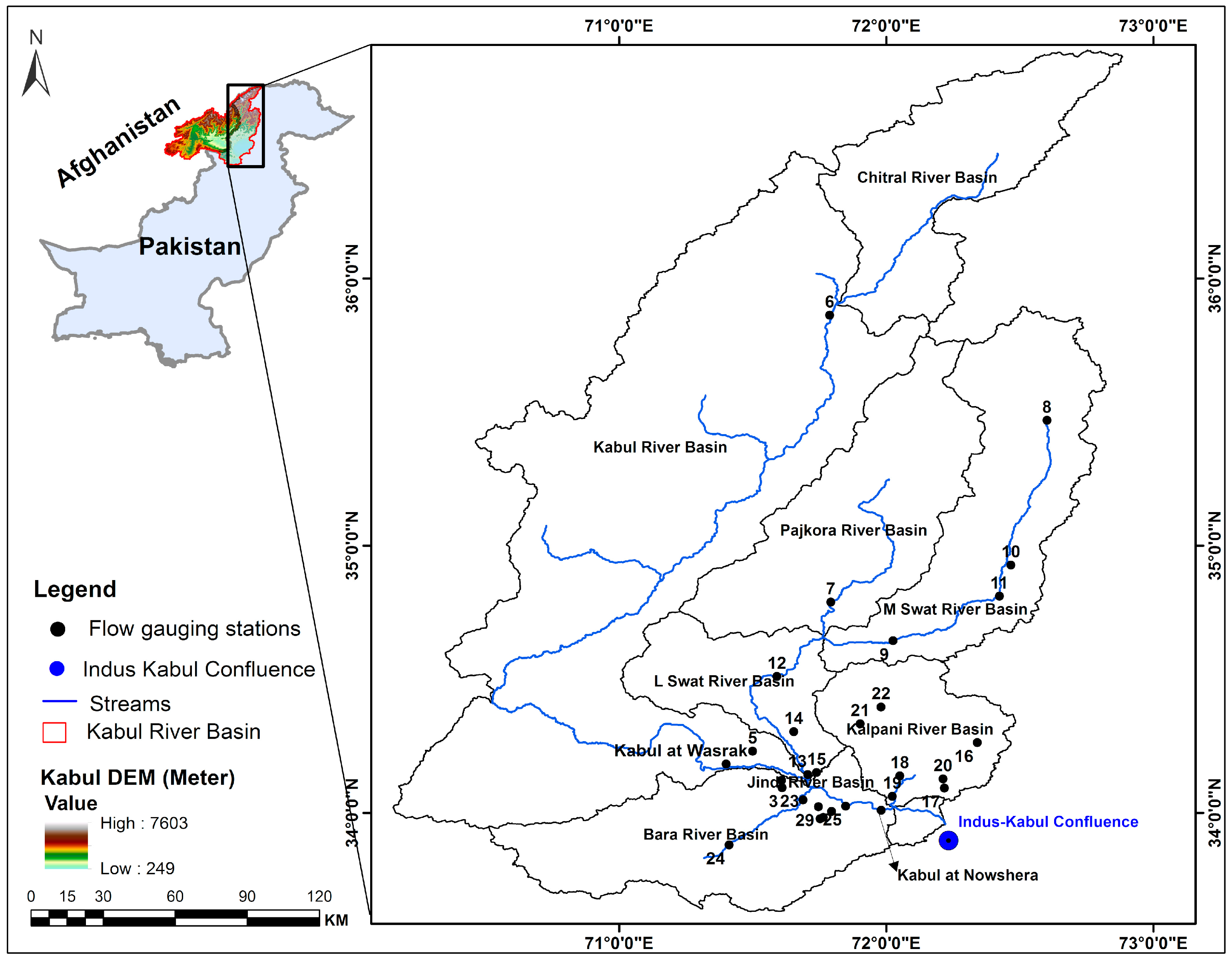
2. Study Area and Data Description

2.1. Study Area

The Kabul River basin (KRB), in Pakistan, stretches from 71°1′55″–72°56′0″ E to 33°20′9″–36°50′0″ N, as shown in Figure 1, which covers an area of 33,709 km². The Kabul River starts at the base of Unai pass from the Hindu Kush Mountains in Afghanistan and flows eastward, covering a distance of 700 km to drain into the Indus River, Pakistan [43]. The entire basin covers an area of 87,499 km². The elevation in the basin varies substantially from 249 m.a.s.l to 7603 m.a.s.l. High elevation mountains are mainly located in the north. The average temperature and average precipitation vary significantly across the River basin. The average temperature is about 13 °C. Most of the precipitation occurs in the northern mountain and highlands, reported up to 1600 mm. [44].

This study explores the part of the KRB that contributes to flooding. The flood problem arises mainly as the Kabul River enters Pakistan. The Logar River basin, Alingar River basin, and Panjshir River basin lie in Afghanistan. Three dams—Naghlu, Surobi, and Darunta—are located in Afghanistan on the Kabul River and Warsak dam is also located on the Kabul River in Pakistan. The study area is further divided into eight sub-basins: Kabul River basin, Chitral River basin, Main Swat River basin, Panjkora River basin, Lower Swat River basin, Kalpani River basin, Jindi River basin, and Bara River basin. The SRTM-DEM (Shuttle Radar Topography Mission–digital elevation model) of 30 m resolution and the geographical location of the sub-basins are also illustrated in Figure 1.

2.2. Flood Data

Twenty-nine flow gauge stations were selected to study the flood regime of the KRB. The annual maximum daily peak flow data for the seven flow gauge stations at main rivers sites were obtained from Surface Water Hydrology Project of Water and Power Development Authority (SWHP–WAPDA). The streamflow data of the remaining study sites were obtained from the Hydrology Section of the Irrigation Department of Khyber Pakhtunkhwa Province, Pakistan. The study sites that had at least 30 years of records were selected. The main characteristics of the sub-basins and the respective flow gauge stations in each sub-basin are presented in

Table 1. Basic information of flow gauges and sub-basins in the KRB, Pakistan.

Site#	Sub Basin and Flow Gauge Stations	Basin Area (km2)	Coefficient of Variation (Cv)	Number of Years of Record
	Kabul River Basin	87,499
1	Kabul River at Warsak		0.292	52 (1965–2016)
2	Kabul River at Nowshera		0.433	55 (1962–2016)
3	Shahalam River		0.724	30 (1987–2016)
4	Naguman River		0.829	30 (1987–2016)
5	Adezai River		0.739	30 (1987–2016)
	Chitral River Basin	11,396
6	Chitral River		0.2	50 (1964–2013)
	Panjkora River Basin	5917
7	Panjkora River		0.859	33 (1984–2016)
	Main Swat River Basin	6066
8	Swat River at Kalam		0.2	59 (1961–2009)
9	Swat River at Chakdara		0.336	49 (1961–2009)
10	Swat River at Khawazakela		0.84	34 (1983–2016)
11	Swat River at Ningolai		1.425	31(1986–2016)
	Lower Swat River Basin	2685
12	Swat River at Munda Head Works		0.744	55 (1962–2016)
13	Khiyali River at Charsada Road		0.815	48 (1969–2016)
14	Jundi Nullah at Tangi		3.06	37 (1974–2011)
	Jindi River Basin	13
15	Jindi River		0.684	48 (1969–2016)
	Kalpani River Basin	2830
16	Naranji Nullah		0.975	49 (1968–2016)
17	Badri Nullah		0.893	45 (1966–2010)
18	Kalpani River at Mardan		1.476	33 (1984–2016)
19	Kalpani River at Risalpur		0.752	33 (1984–2016)
20	Dagi Nullah		1.01	33 (1984–2016)
21	Bagiari Nullah		0.917	30 (1987–2016)
22	Lund Khawar West		1.13	30 (1987–2016)
	Bara River Basin	3388
23	Budni Nullah		1.28	43 (1974–2016)
24	Bara River at Kohat Bridge		1.69	34 (1983–2016)
25	Khuderzai Nullah		1.65	32 (1980–2011)
26	Chillah Nullah at Pabi		1.15	32 (1980–2011)
27	Hakim Garhi Nullah		0.6	31 (1980–2010)
28	Wazir Garhi Nullah		1.69	30 (1981–2010)
29	Muqam Nullah		0.781	30 (1981–2010)

and Figure 1 describes the geographical locations of the flow gauge stations in each sub-basin.

2.3. Flood Generating Mechanism in KRB

The hydrology of floods is linked to weather and climate as well as to physiographical features [45]. The basin has large altitudinal variations from 249 m.a.s.l. to 7603 m.a.s.l. Glacier-melt contribution from the upper part of the basin combined with rainfall in the lower part is the most likely cause of flooding in the region [38]. In the KRB, floods are mostly generated by monsoon rainfall but snow or glacial melt floods have also been observed in some parts of the basin. Snowmelt floods are not common. According to the data used in this study, all of the flood peaks were observed during the monsoon season, from July to August, in almost all the tributaries of the KRB. The historical floods occurred in July 2010, August 1995, and July 1992; all were observed during the monsoon. Anjum et al. [46] provided the details regarding rainfall magnitude, intensity, and spatial extent for the 2010 event. The South Asian monsoon originating from the Bay of Bengal is the dominant weather system for flood generation in the KRB.

However, the flood of 2005 in the Kabul and Indus Rivers was due to snowmelt as well as rainfall in the pre-monsoon period [47]. The flooding behavior of the different tributaries differs according to their catchment characteristics. The riverine floods in the Kabul River usually start below the Warsak dam, and this phenomenon propagates until its confluence with the Indus River at Khairabad near Attock. Riverine floods also occur in the Swat River in the Lower Swat catchment. In the rest of the KRB, flash flooding is a common disaster, along with landslides and torrential rains [45].

3. Methods

3.1. Preliminary Analysis

3.1.1. Trend Analysis

The non-parametric rank-based Mann–Kendall (MK) [48,49] test was used to detect trends in annual maximum flood series. The trend analysis was performed to show a clear understanding of the whole study area, while an objective criterion (means if statistically significant trend exists) was adopted for the non-stationary modeling of flood regime. The Mann–Kendall test was applied at different significance levels. The autocorrelation function (ACF) was also computed, before applying the Mann–Kendall (MK) test to check the presence of serial correlations in the annual maximum flood series.

3.1.2. Selection of Extreme Value Distribution

The Bayesian method using the GEV distribution is getting attention for analyzing hydrological extremes. The current study also utilized the GEV distribution, which is the integration of Gumbel, Fréchet, and Weibull distributions, and developed on the limit theorems for block maxima or annual maxima [50]. Mathematically, the cumulative distribution of the GEV can be written as [51]:

$$\psi \left(x\right)=exp\left\{-{\left(1+\xi \left(\frac{x-\mu }{\sigma }\right)\right)}^{\frac{-1}{\xi }}\right\}, \left(1+\xi \left(\frac{x-\mu }{\sigma }\right)\right) > 0,$$

(1)

where ψ(x) is expressed as $\left(1+\xi \left(\frac{x-\mu }{\sigma }\right)\right)$ > 0; somewhere else, ψ(x) is either 0 or 1 [52].

The location parameter (µ), describes the center of the GEV distribution, the scale parameter (σ) describes the deviation around (µ), and the shape parameter (ξ) describes the tail behavior of the distribution. When ξ → 0, ξ < 0, and ξ > 0, GEV approaches the Gumbel, Weibull, and Fréchet distributions, respectively.

3.1.3. Goodness of Fit Statistics to GEV Distribution

The goodness of fit analysis of annual maximum peak flow data to the GEV distribution was performed in order to investigate whether the historical data belonged to the said GEV distribution. The Anderson–Darling (AD) [53] and Kolmogorov–Smirnov (K-S) [54] tests were performed for this purpose, using an EasyFit software (version 5.6, MathWave Technologies) [55]. EasyFit estimated the parameters of the GEV distribution based on maximum likelihood (ML) estimation, using equal probability sampling. The parameters estimated using the EasyFit software were used to assess the goodness of fit by AD and K-S statistics.

The K-S statistic (D) is based on the largest vertical difference between the theoretical and the empirical cumulative distribution function as shown below:

$$D = m_{1\le i\le n}\left(\psi (x_i\right)- \frac{i-1}{n},\frac{i}{n}- \psi \left(x_i\right)).$$

(2)

The Anderson–Darling procedure compares the fit of an observed cumulative distribution function to an expected cumulative distribution function. This test gives more weight to tails than the K-S test.

$$A^2= -n-\frac{1}{n} {\sum }_{i=1}^n\left(2i-1\right)\times [\ln \psi (x_i)+\ln \left(1-\psi \left(x_{n-i+1}\right)\right)].$$

(3)

H₀: The data follow the specified distribution;

H_a: The data do not follow the specified distribution.

The hypothesis regarding the distributional form was rejected at the significance level of 0.05 (alpha) if the test statistic, A² or D, was greater than the critical value of 2.5018 and 0.18482, respectively.

Moreover, the outlier’s detection in the annual extreme data of flood series was also performed using the Chauvenet’s Criterion [56].

3.2. Model Design

The extreme value theory of stationary random process is based on that the statistical properties of extremes—here, the distribution parameters θ = (µ, σ, ξ) are free from time dependency [57], while in a non-stationary random process, the parameters of the said distribution function rely on time-dependency, and the properties of the distribution also vary with time [58]. For this study, two cases were considered.

(1)

Stationary Case: all the model parameters were considered constant.

(2)

Non-stationary Case: the location parameter (µ) was considered a function of time, as shown in Equation (4), while scale and shape parameters were kept constant:

$$\mu \left(t\right)= {\mu }_{1}t+{\mu }_0,$$

(4)

where t is time, θ = (µ₁, µ₀) are the regression parameters [50,57,58,59,60]. The location parameter was calculated for each study site in the stationary case and non-stationary case.

3.2.1. Bayes Theorem for GEV Distribution

Let θ be the parameter of given distribution and let Y = {y₁, y₂, …, y_n} be the set of n observations. According to the Bayes theorem, the probability of θ given Y (posterior) is proportional to the product of the probability of θ (prior) and the probability of Y given θ (likelihood function). Assuming the independence between the observations, Y:

$$P\left(\theta |Y\right)\propto {\displaystyle \prod }_{i=1}^{n}P\left(\theta \right) \times P\left(y_i|\theta \right).$$

(5)

Here, the likelihood function is the GEV distribution and θ is the vector containing the parameters of GEV distribution to be estimated. In the stationary case, θ = (µ, σ, ξ). By assuming independent GEV parameters:

$$P\left(\mu ,\sigma ,\xi |Y\right)\propto {\displaystyle \prod }_{i=1}^{n}P(\mu )\times P\left(\sigma \right)\times P\left(\xi \right) \times P\left(y_i|\mu ,\sigma ,\xi \right) .$$

(6)

In the case of non-stationary analysis, θ contains an additional parameter, which is time-dependent here, i.e., $\mu \left(t\right)$, hence, the Bayes theorem for estimation of GEV parameters under the non-stationary case can be expressed as [57,60]:

$$P\left(\theta |Y, t\right)\propto {\displaystyle \prod }_{i=1}^{n}P\left(\theta \right) \times P\left(y_i|\theta ,t\right).$$

(7)

The resulting posterior distributions $P\left(\theta |Y,t\right)$ provide information on the distribution parameters (µ₁, µ₀, σ, ξ).

3.2.2. Prior Distribution

A Bayesian model utilizes a prior belief to calculate the posterior belief. For the current study, we utilized NEVA (non-stationary extreme value analysis, Matlab Package) [60,61,62] for our analysis. In NEVA, the priors are non-informative normal distributions, for location and scale parameters, while the priors for the shape parameter are a normal distribution, with a standard deviation of 0.3, as suggested by [57,60,62]. Initially, the shape parameter was considered a non-informative prior:

ξ ~ N (−5, 5),

(8)

if the value of the shape parameter in the posterior distribution exceeded beyond the plausible limit (−5, 5), as suggested by Martins and Stedinger [63]. Then, we modified the priors for shape parameter, considering partial pooling of information across sites that had similar flood types, for improving the flood quantiles estimates for “at site modeling” using the regional information. The shape parameter was considered an informative prior and the range of priors for shape parameter was:

ξ ~ N (0, Ksi).

(9)

where, the Ksi stands for the shape parameter value of the site of interest from where it was exchanged. However, the location and scale parameter across sites were not shared.

3.2.3. Parameters Estimation and Convergence Criterion

To estimate the parameters inferred by Bayes, the Differential Evolution Markov Chain (DE-MC) is integrated to generate a large number of realizations from the parameters’ posterior distributions [64,65]. The DE-MC attributes to the genetic algorithm Differential Evolution (DE) for global optimization over real parameter space with the Markov Chain Monte Carlo (MCMC) approach [64,65]. Here, the target posterior distributions were sampled through five Markov Chains constructed in parallel. These chains were allowed to learn from each other by generating candidate draws based on two random parent Markov Chains, rather than running independently. Therefore, it had the advantages of simplicity, speed of calculation, and convergence over the conventional MCMC. The initial numbers of burned samples were 6000 and numbers of evaluations were 10,000 for each study site. The R-hat criterion, suggested by Gelman and Shirley [66], was used to assess convergence, where R-hat should remain below 1.1.

Uncertainty estimates for FFCs are crucial for risk assessment and decision making. By combining DE-MC with Bayesian inference, the posterior probability intervals or credible intervals and uncertainty bounds of estimated return levels based on the sampled parameters could be obtained simultaneously for FFCs. For example, for a time series of annual maximum peak flow, the time-variant parameter (µ(t)) was derived by computing the 95th percentile of DE-MC sampled µ(t), (i.e., the 95th percentile of µ(t = 1), …, µ(t = 100)). These model parameters were then used to develop the stationary and non-stationary FFCs.

FFCs could also be drawn at 50% Bayesian credible intervals or at any other desired intervals.

3.2.4. Model Evaluation

In order to evaluate the suitability of the stationary versus non-stationary models, a Bayes factor K was calculated based on the posterior distributions of sampled parameters of both models. The stationary model was considered a null model M1, while the non-stationary model M2 was considered an alternative.

A value of Bayes factor > 1 denotes the stationary model is favored, while a value < 1 argues in the favor of the non-stationary model. Similarly, a value approaching +infinity favors the stationary model, and −infinity favors non-stationary models. Equation (10) represents the computation of Bayes factor, as follows:

$$K= \frac{Pr(DA|M1)}{Pr(DA|M2)}= \frac{\int Pr({\theta }_1|M1)Pr\left(DA|{\theta }_{1}M1\right)d{\theta }_1}{\int Pr({\theta }_2|M2)Pr(DA|{\theta }_{2}M2)d{\theta }_2}.$$

(10)

The term DA denotes input data, and θ stands for model parameters. The term Pr (DA|M) can be expressed using Monte Carlo integration estimation as follows:

$$Pr\left(DA|M\right)={\left\{\frac{1}{m}{\displaystyle \sum }_{m_{i=1}}Pr{(DA|{\theta }^{\left(i\right)},M)}^{-1}\right\}}^{-1}.$$

(11)

For more details see [67].

4. Results and Discussion

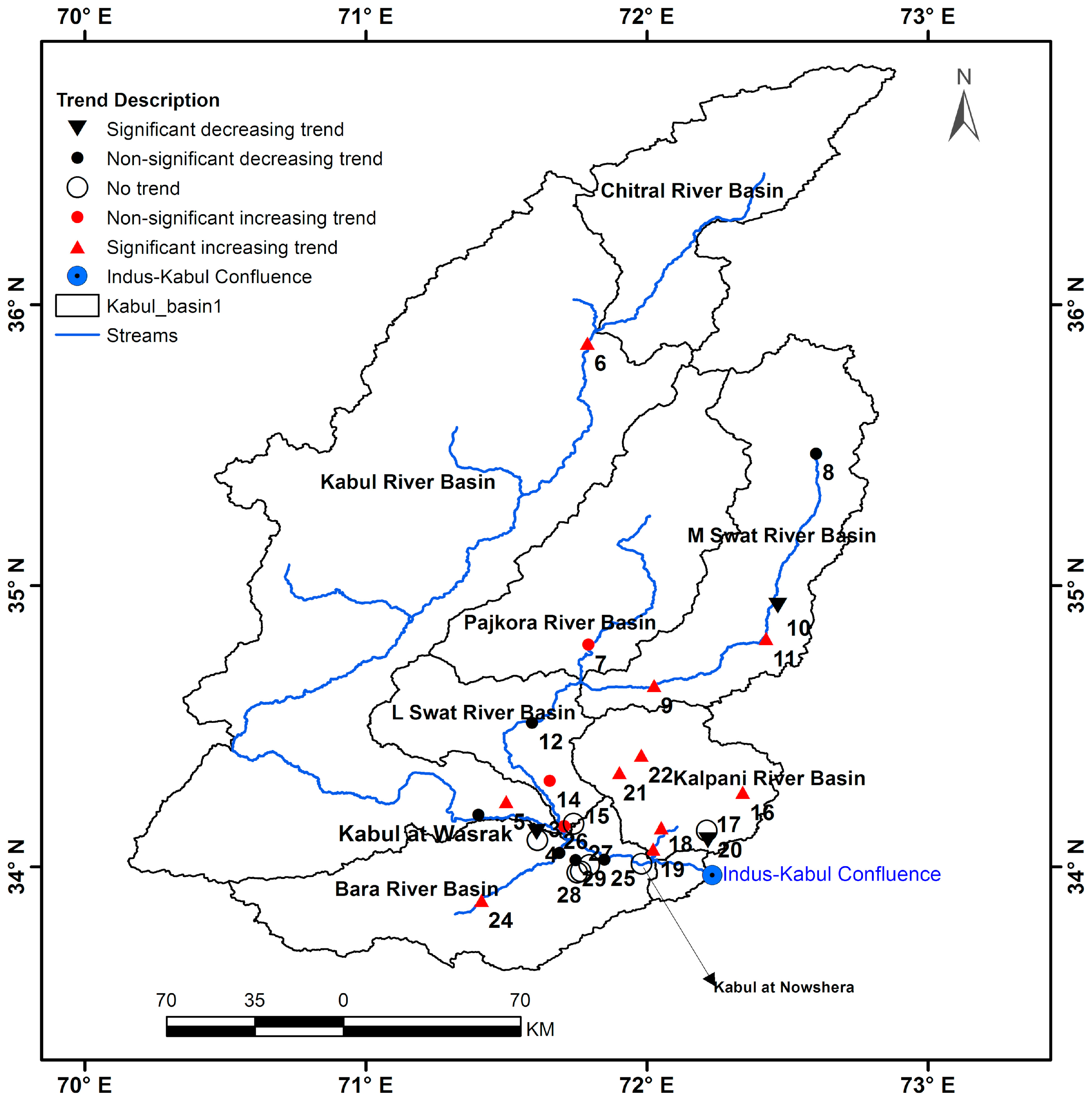
4.1. Temporal and Spatial Trends in Flood Regime

The trend magnitude for each station is presented in

Table 2. Description of trends in the annual maximum flood regime across the KRB, Pakistan.

Site #	Mann–Kendall (Test-Z)	Site #	Mann–Kendall (Test-Z)	Site #	Mann–Kendall (Test-Z)
1	−1.54	11	4.78 ***	21	3.28 **
2	−0.35	12	−0.89	22	2.83 **
3	0.41	13	1.18	23	−1.28
4	−2.02 *	14	0.86	24	2.28 *
5	2.61 **	15	−0.37	25	−1.19
6	2.80 **	16	1.79 +	26	−0.67
7	0.93	17	−3.07 **	27	0.34
8	−1.36	18	3.24 **	28	−0.54
9	1.73 +	19	2.13 *	29	−0.83
10	−2.36 *	20	0.16

*** Trend is significant at α = 0.001, ** Trend is significant at α = 0.01, * Trend is significant at α = 0.05, ⁺ Trend significant at α = 0.1.

. Trend analysis results demonstrated the significant trend by 37.93% of the flow gauge stations in the entire basin; among them, 27.6% showed a significant increasing trend at the 0.05 significance level and 10.34% of the stations showed a significant decreasing trend at the significance level of 0.05. Moreover, 6.9% of the flow gauge stations also revealed a significant increasing trend at the significance level of 0.1. Non-significant trends were also exhibited by 31% of the flow gauge stations. The Chitral River at Chitral, the Kalpani River at Risalpur, the Kalpani River at Mardan, the Swat River at Chakdara, the Swat River at Ningolai, the Adezai River, the Naranji Nullah, the Bagiari Nullah, the Lund Khawar West, and the Bara River at Kohat Bridge displayed a significant increasing trend (Site #5, 6, 9, 11, 16, 18, 19, 21, 22, and 24), while the Swat River at Khawazakhela, the Naguman River, and the Badri Nullah showed a significant decreasing trend. The Khiyali River, the Panjkora River, and the Jundi Nullah at Tangi represented a moderate increasing trend, while the Kabul River at Warsak, the Swat River at Kalam, the Swat River at Munda Head Works, the Budni Nullah, and the Khuderzai Nullah displayed a moderate decreasing trend. Moreover, the main flow gauge station—the Kabul River at Nowshera—did not show any significant trend.

Figure 2 represents the basin-wide spatial distribution of trends in the flood regime, which showed that the flood regime of the Chitral River, the Kalpani River, and the Main Swat River basins exhibited significant increasing trends. However, the Swat River at Khawazakhela and the Badri Nullah represented a significant decreasing trend.

The Lower Swat River, the Kabul sub-basin, and the Jindi River basins showed non-significant trends.

Especially for the southwestern part of the KRB, the Bara River at Kohat Bridge showed non-stationarity in the flood regime due to a significant increasing trend, while all other flow gauge stations in the Bara River basin showed insignificant trends.

The change in flood regime was found to be more evident for the northern and northeastern part of the KRB as compared to the central and southwestern parts of the KRB. Consequently, the overall basin showed large spatial variations. However, the basin did not represent a regular spatial pattern. These spatial variations may be due to climatology, topography, and complex orography of the KRB in the HKH region. However, the temporal changes in the flood regime might be attributable to regional environmental change. The results of trend analysis were consistent with previous studies [68,69,70], but these studies used only two to three flow gauges.

4.2. Evaluation of Goodness of Fit for Annual Extreme Data of Flood

An objective criterion as suggested by Rosner et al. [71] was adopted to evaluate the goodness of fit of the annual maximum flood series, with GEV and non-stationary temporal trend modeling of the flood regime, i.e., only the sites showing significant trends in their flood regime were selected. The study sites under consideration showed proper fitting using the AD test and the value of test statistics for all the sites using the AD test was less than the critical value of 2.5018. While using the K-S test, all the sites showed proper fitting except site 21, but it was included in the analysis because it satisfied the AD test.

Table 3. The goodness of fit statistics of annual maximum daily peak flow to generalized extreme value (GEV) distribution.

Site #	Gauge Stations	GEV Parameters	Anderson–Darling Test	Kolmogorov–Smirnov Test
			A-D Statistics	K-S Statistics	p-Value
5	Adezai River	ξ = 0.07899 σ = 454.66 µ = 521.18	0.6903	0.15394	0.43251
6	Chitral River	ξ = 0.00307 σ = 143.37 µ = 1026.5	0.22503	0.06435	0.97732
9	Swat River at Chakdara	ξ = 0.13247 σ = 152.1 µ = 646.8	0.66053	0.10305	0.59055
11	Swat River at Ningolai	ξ = 0.52162 σ = 103.82 µ = 83.499	0.60066	0.1453	0.48501
16	Naranji Nullah	ξ = 0.25789 σ = 77.168 µ = 81.939	0.19219	0.06263	0.98424
18	Kalpani River at Mardan	ξ = 0.55205 σ = 106.9 µ = 77.204	1.2218	0.17818	0.21796
19	Kalpani River at Risalpur	ξ = 0.20781 σ = 441.0 µ = 604.88	0.42201	0.10944	0.7987
21	Bagiari Nullah	ξ = 0.06073 σ = 112.05 µ = 94.608	1.838	0.22761	0.08399
22	Lund Khawar West	ξ = 0.37899 σ = 3.7993 µ = 3.164	0.48511	0.12903	0.7523
24	Bara River at Kohat Bridge	ξ = 0.57308 σ = 16.871 µ = 9.4788	1.2595	0.15782	0.33006

provides the results of the test statistics and estimated GEV parameters using ML. The p-value belongs to K-S test only.

Outliers were also detected in the data of the annual maximum flood series for the KRB.

Table 4. Representation of detected outliers, as per Chauvenet’s criterion.

Site #	Station Name	Historical Extreme (Outliers)	Observed Value	Critical Value
5	Adezai River	2285	2.449	2.394
6	Chitral River	1633/1603	2.941/2.76	2.576
9	Swat River at Chakdara	1918/1602	4.6/3.35	2.576
11	Swat River at Ningolai	1475	3.447	2.406
16	Naranji Nullah	850	4.748	2.576
18	Kalpani River at Mardan	1499	3.182	2.429
19	Kalpani River at Risalpur	3358	3.316	2.418
21	Bagiari Nullah	473	2.102	2.394
22	Lund Khawar West	37	3.235	2.394
24	Bara River at Kohat Bridge	331	4.234	2.44

demonstrates the outliers present in the data of selected study sites. Sites 5, 6, 16, 18, 19, 21, and 24 displayed the extreme flood of 2010 as an outlier in the data. Site 6 also revealed the flood of 2005 (1603 m³ s⁻¹) as an outlier, as per evaluation criterion. Similar to site 6, site 9 also represented two outliers in its flood series. The outlier 1918 m³ s⁻¹ represents the flood of 1992, and the corresponding value of 1602 m³ s⁻¹ represents the flood of 1987 for site 9.

For Site 11, the 1475 m³ s⁻¹ value corresponds to the flood of 2016 in the Swat River basin, the sub-basin of the KRB. The flood discharge of 37 m³ s⁻¹ at Lund Khawar West (Site 22) in 1997 was also recorded as an outlier. Despite the existence of outliers, the data series belongs to the GEV distribution as per AD and K-S test statistics.

4.3. Regionalization of Shape Parameter for Flash Floods Across the KRB

The shape parameter of the GEV distribution is important for the estimation of flood quantiles. Initially, non-informative priors for shape parameter were used for the Bayesian analysis of annual maximum flood regime for the selected study sites that had non-stationarity, due to the existence of temporal trends. About 30% of the study sites yielded a value of shape parameter in posterior distribution that exceeded beyond the plausible limit (−5, 5) as suggested by Martins and Stedinger [63], causing the degeneration of the GEV distribution. In order to avoid this, homogeneous sites were identified. Halbert et al., Kuczera, Kyselý et al., Sun et al., and Viglione et al. [72,73,74,75,76] state that the use of regional information will improve the flood frequency estimation and reduce the uncertainty for sites having short records.

Table 5. Correlation matrix for the selected study sites.

Site #	5	6	9	11	16	18	19	21	22	24
5	1	0.24	−0.04	0.63	0.35	0.61	0.14	0.25	0.39	0.48
6	0.24	1	0.29	0.11	0.42	0.33	0.42	0.37	0.38	0.41
9	−0.04	0.29	1	0.11	0.11	−0.05	−0.22	−0.02	−0.17	0.04
11	0.63	0.11	0.11	1	0.2	0.59	0.04	0.49	0.6	0.21
16	0.35	0.42	0.12	0.2	1	0.41	0.47	0.29	0.32	0.63
18	0.61	0.33	−0.05	0.59	0.41	1	0.63	0.53	0.52	0.54
19	0.14	0.42	−0.22	0.04	0.47	0.63	1	0.65	0.64	0.42
21	0.25	0.37	−0.02	0.49	0.29	0.53	0.65	1	0.41	0.2
22	0.39	0.38	−0.17	0.6	0.32	0.52	0.64	0.41	1	0.47
24	0.48	0.41	0.04	0.21	0.63	0.54	0.42	0.2	0.47	1

illustrates the correlation matrix for the selected study sites, which demonstrates that hierarchical clustering is possible based on the correlation between the annual maximum flood series of the selected study sites.

A positive correlation is present between the sites. Although site 9 possesses the least positive correlation with site 6, site 6 has more positive correlations with other sites, hence why all the sites are considered homogenous. All the sites also possess “flash” flood type. Moreover, all the sites could also be considered homogenous because of the existence of trends in their flood regime. Sun et al. [77] also highlighted the clustering of temporal trends and exchange of shape parameter for the Bayesian analysis of annual maximum floods across Germany.

Furthermore, the utilization of ML for the estimation of the shape parameter for GEV distribution was found reliable for large records—at least 50 year [78]. After considering all the study sites as homogenous based on the correlations between sites, similar flood type, and existence of trends, Naranji Nullah (site 16), with a sufficiently long record, was considered the benchmark site. The shape parameter estimated by ML was approximately 0.26 for site #16. This value of shape parameter (0.26) was further recognized for all the study sites as an informative prior in the Bayesian model. This is like partial pooling of information across homogenous sites, which ultimately improved the flood quantiles estimates using the regional information as compared to non-informative priors on shape parameter. Lima et al. [79] used the basin’s average shape parameter value in local and regional hierarchical Bayesian models to solve the issue of sites where the shape parameter value exceeds beyond (−5–5). Lima et al. [79] used the prior for shape parameter as non-informative, but this study considers the priors on shape parameter to be informative priors.

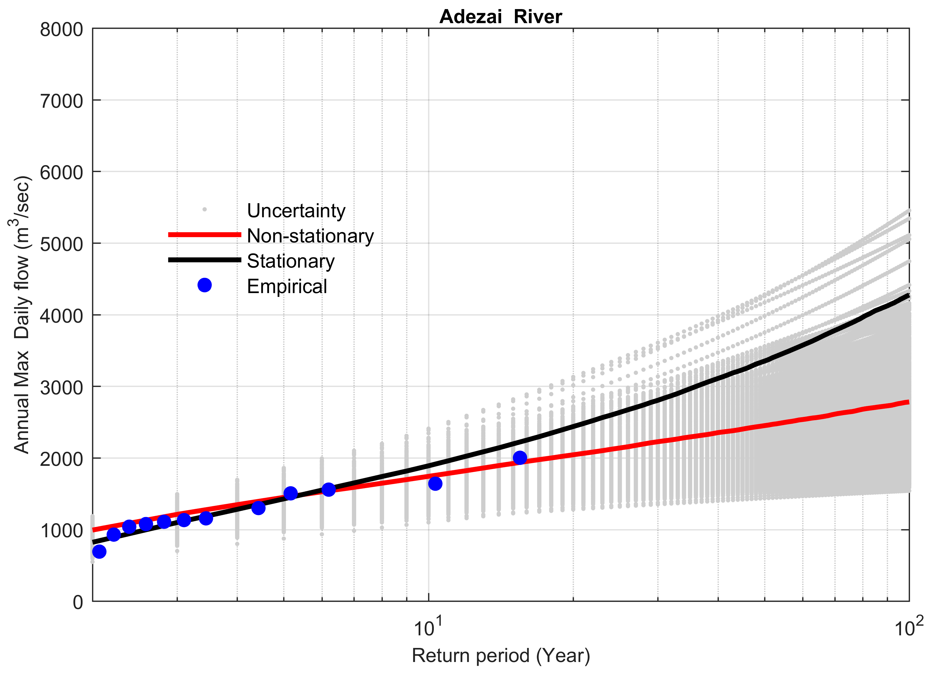
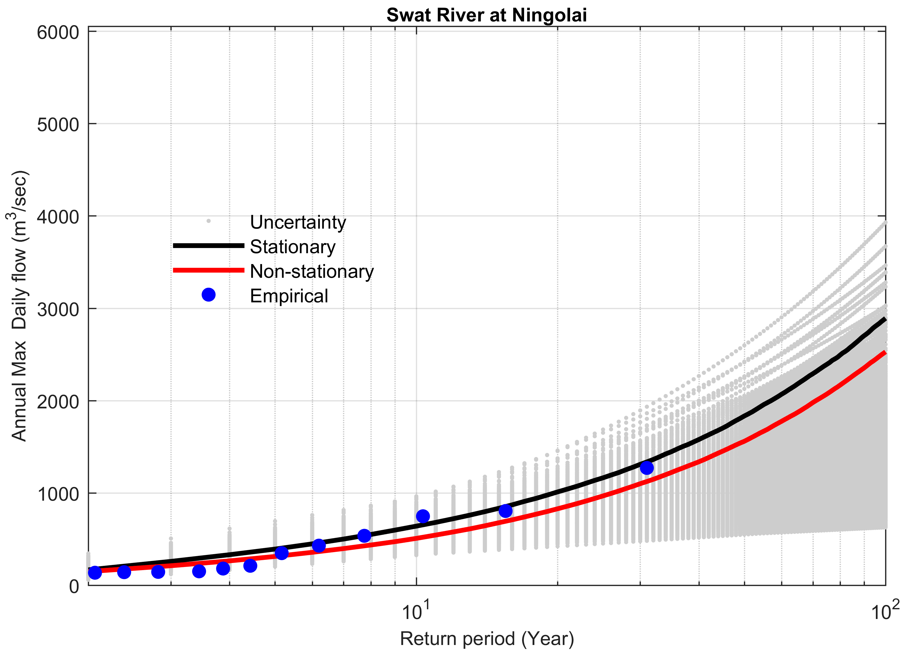
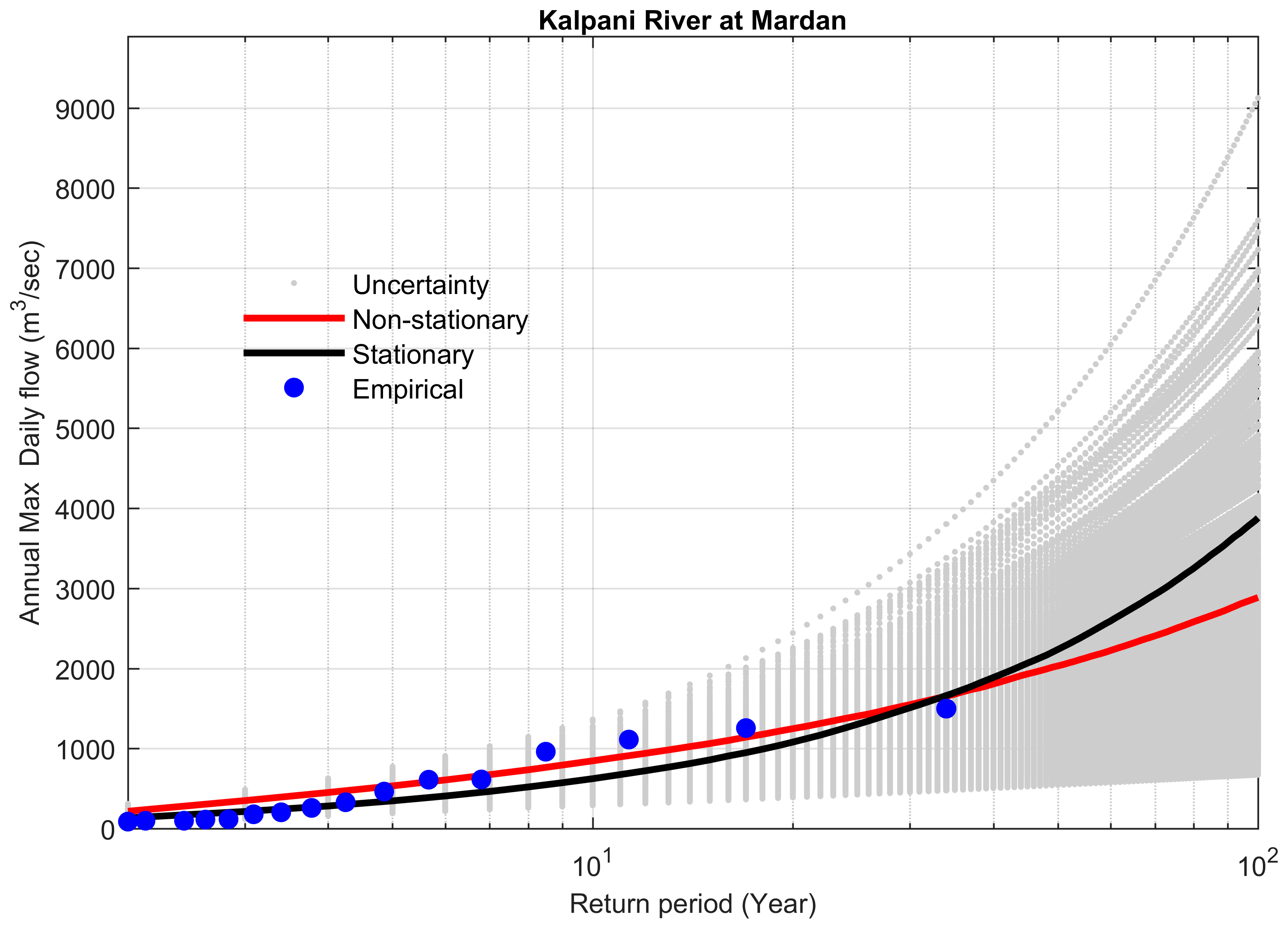
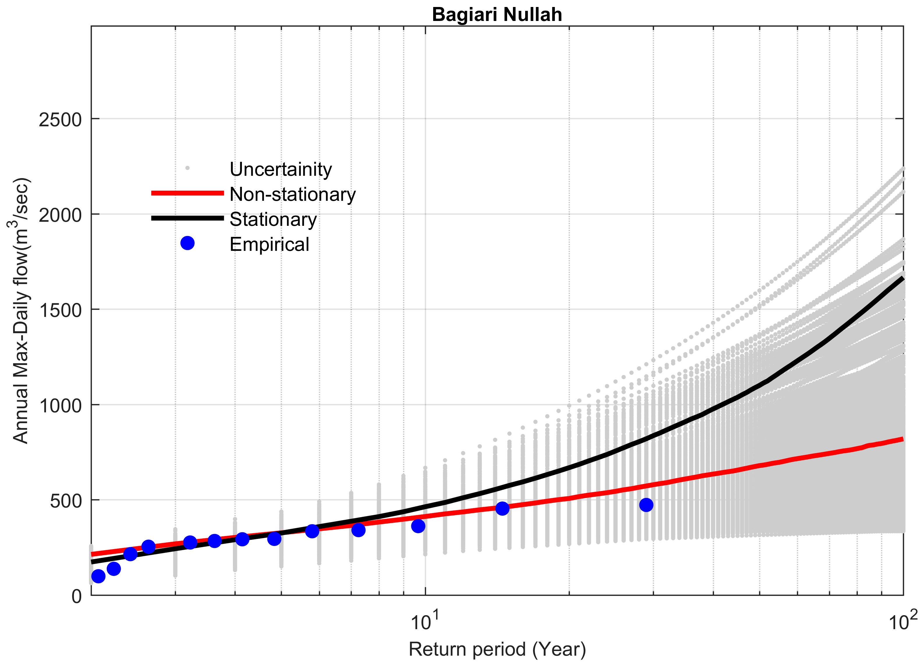
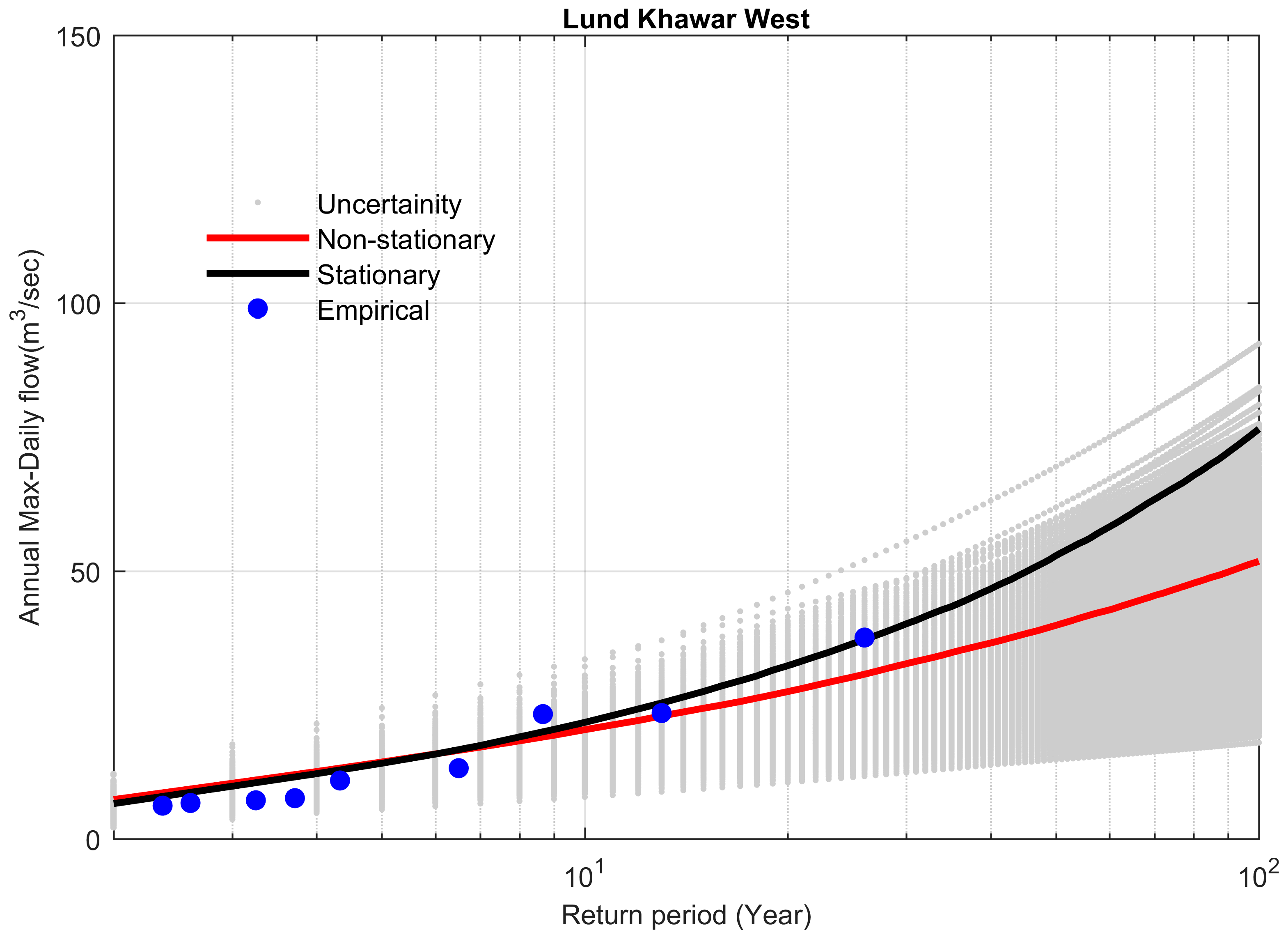
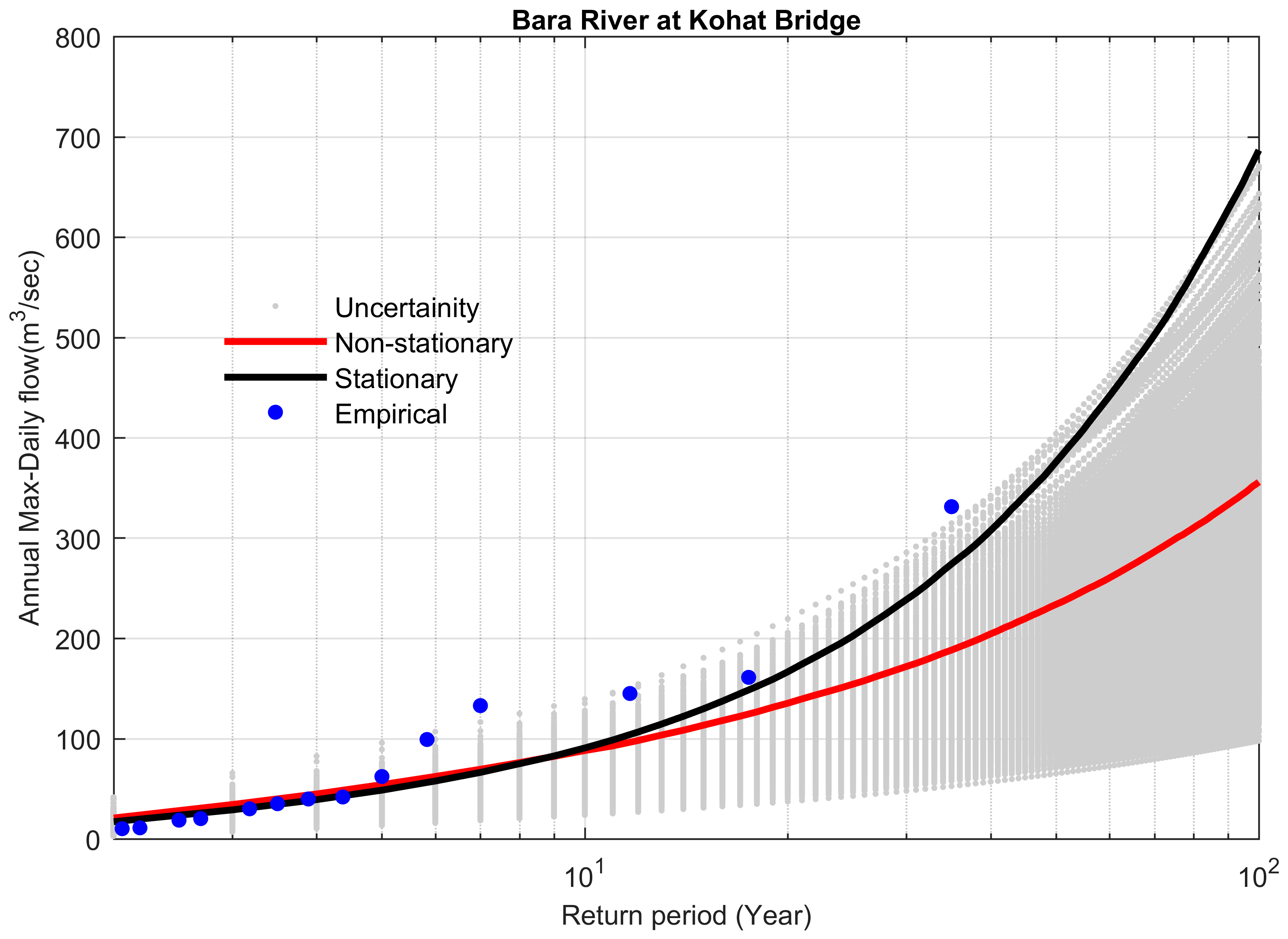
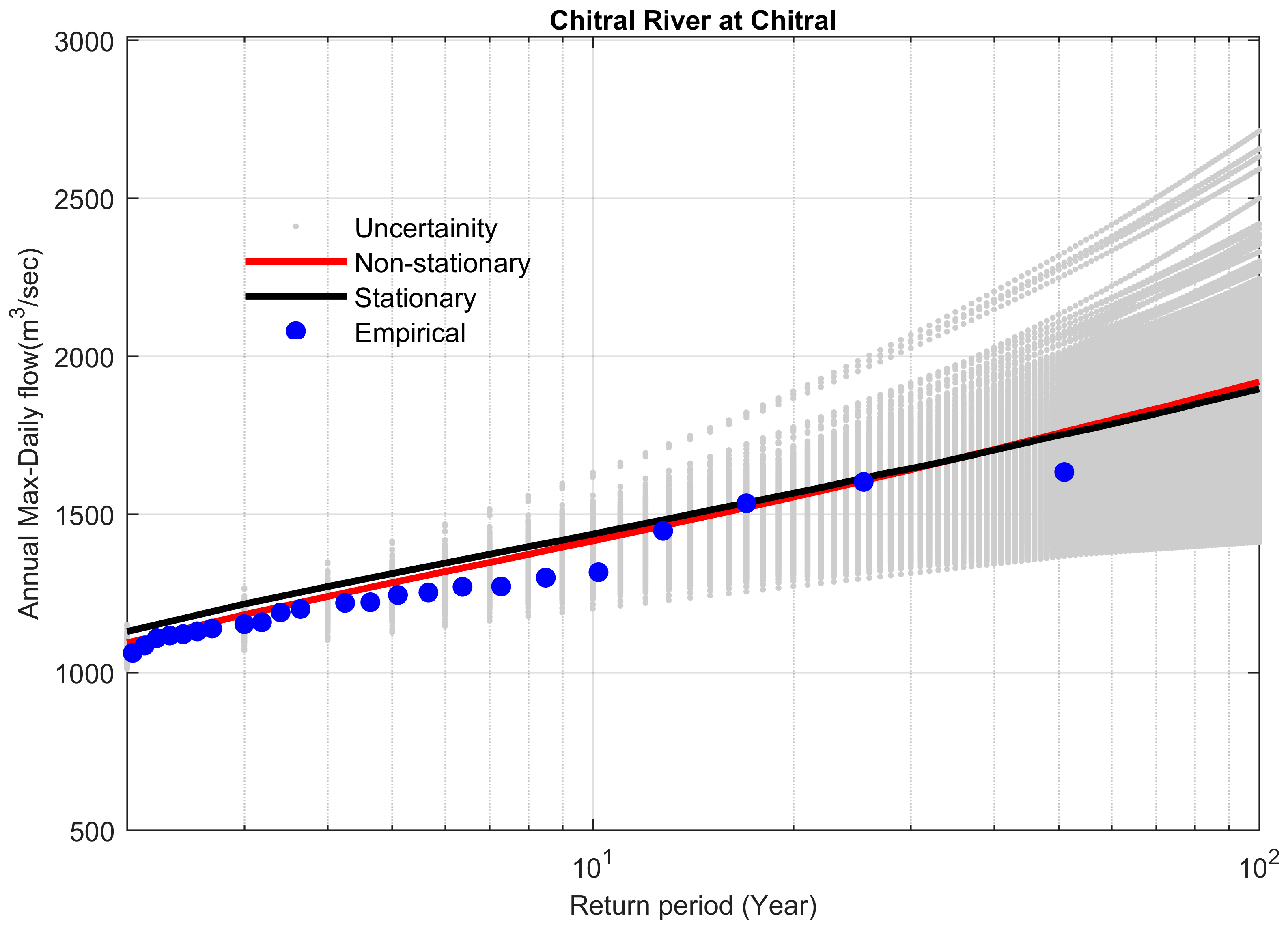
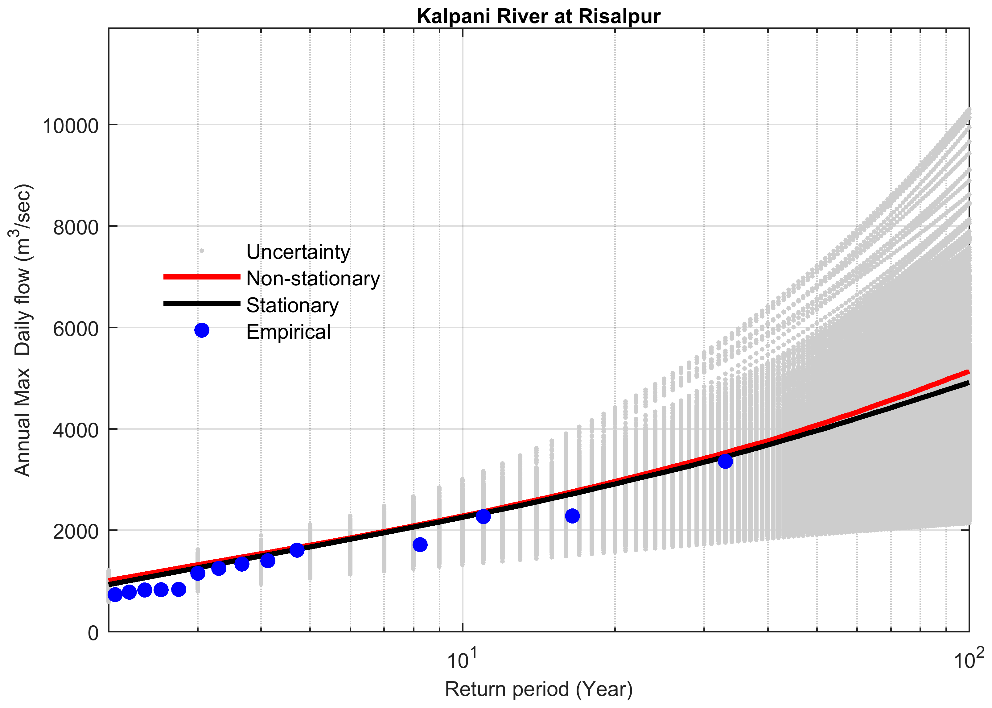
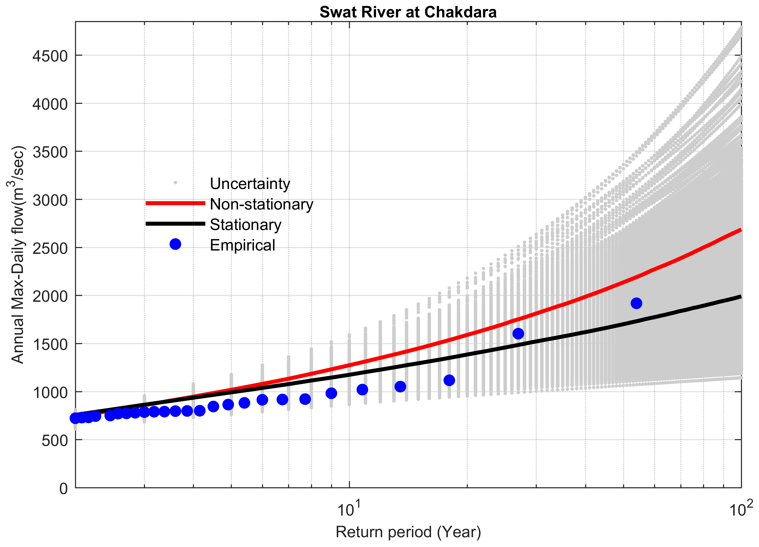
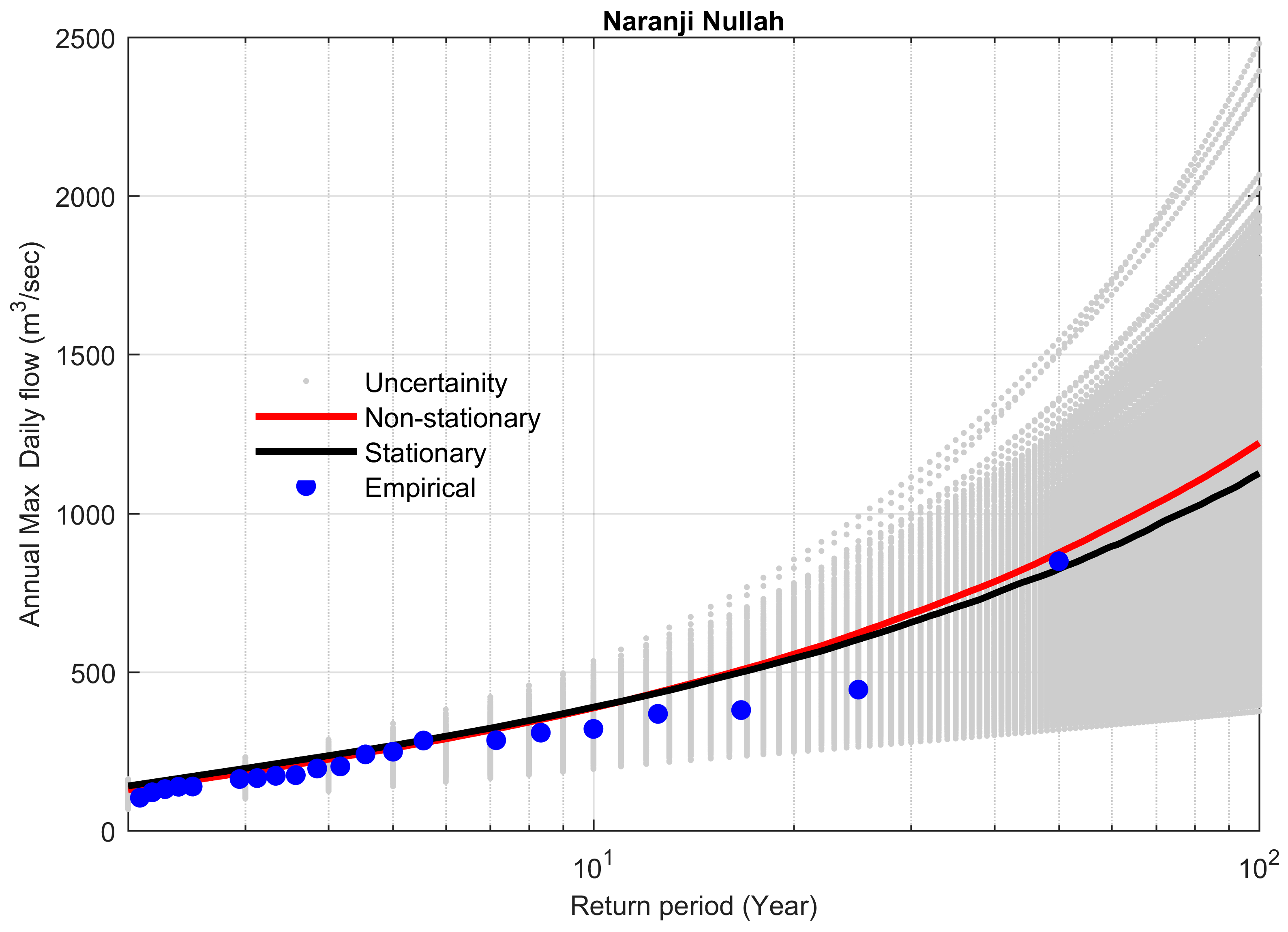
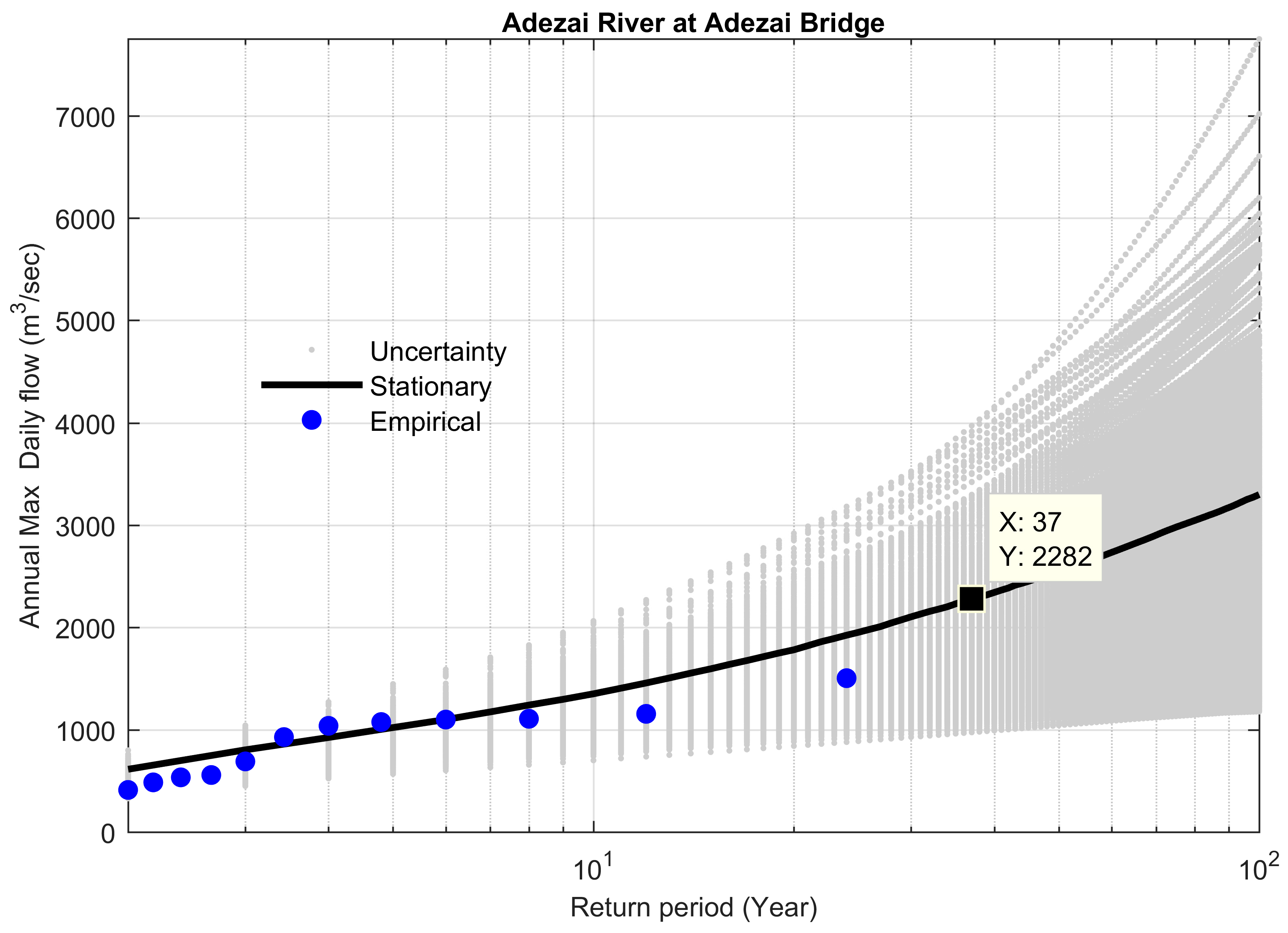
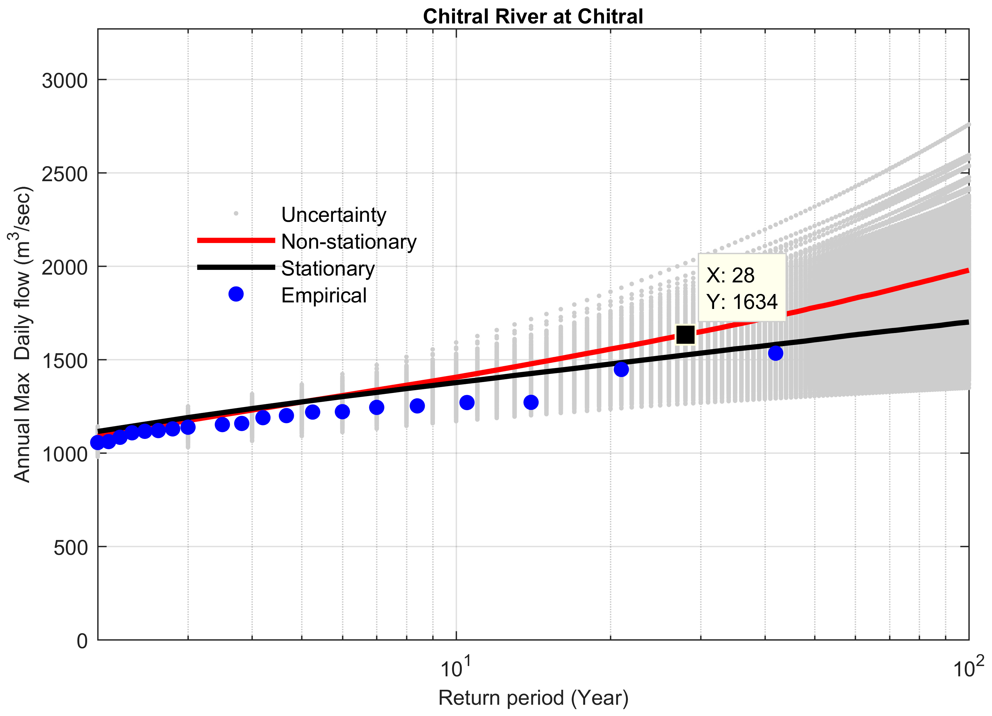
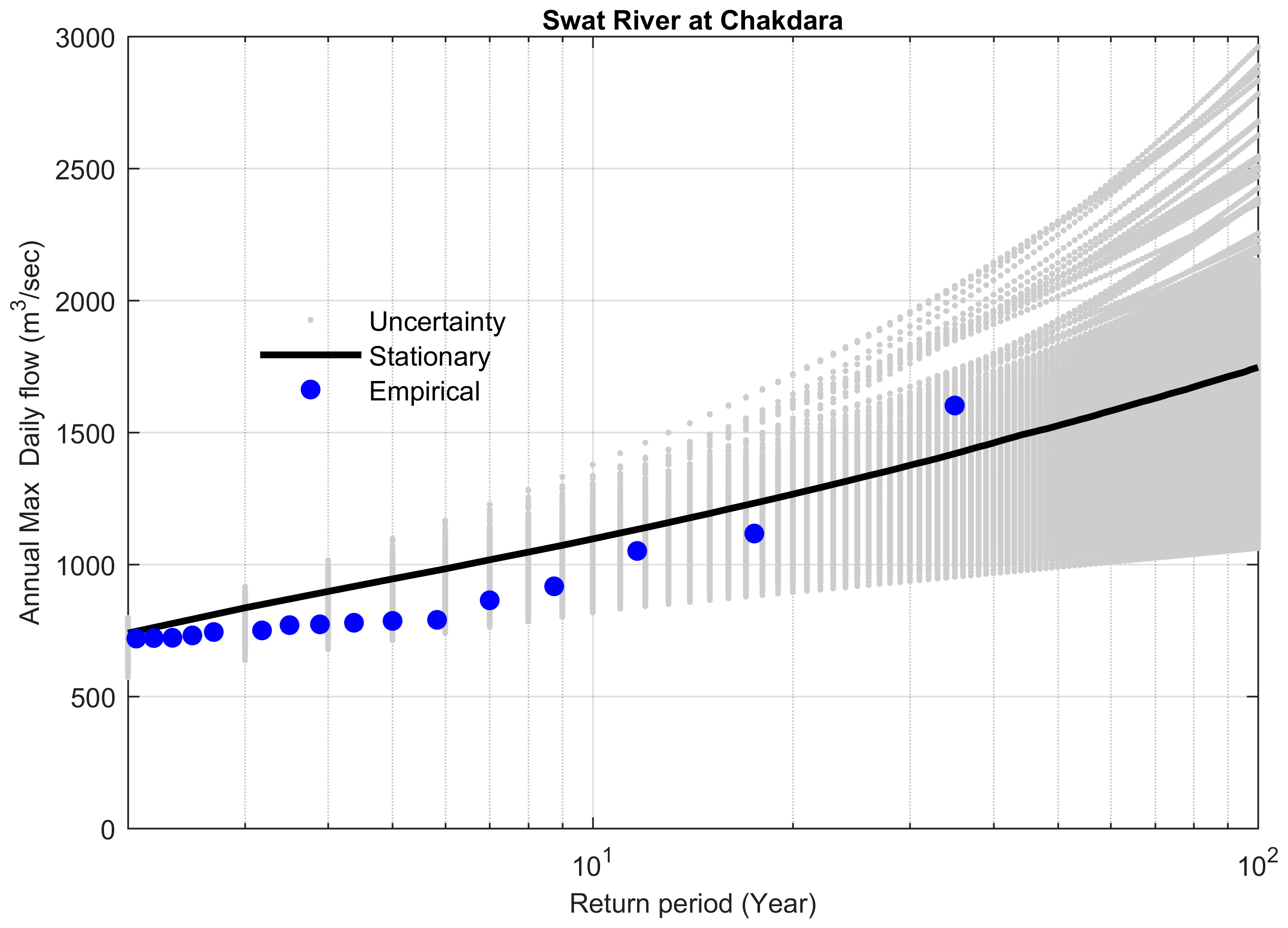
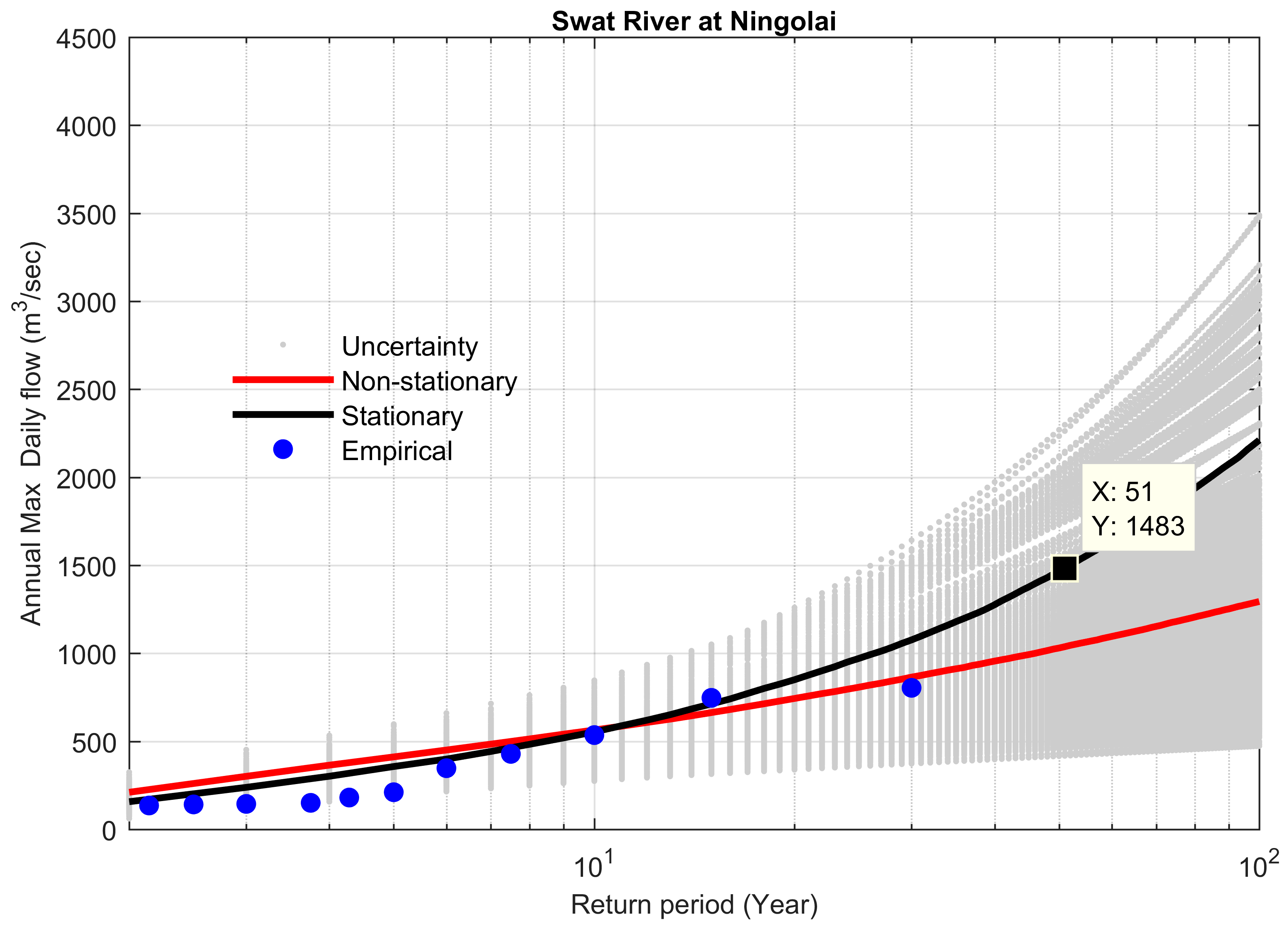
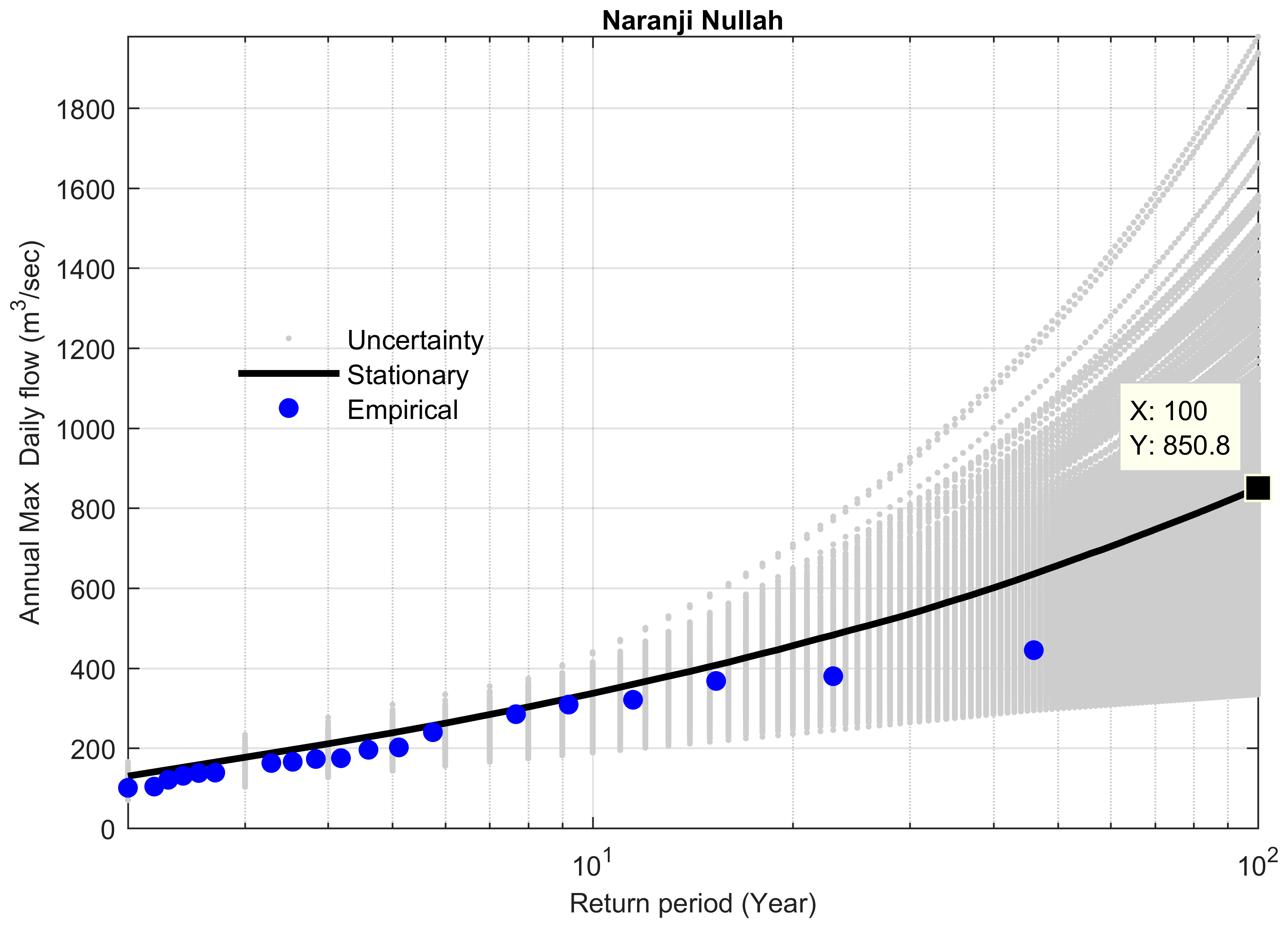
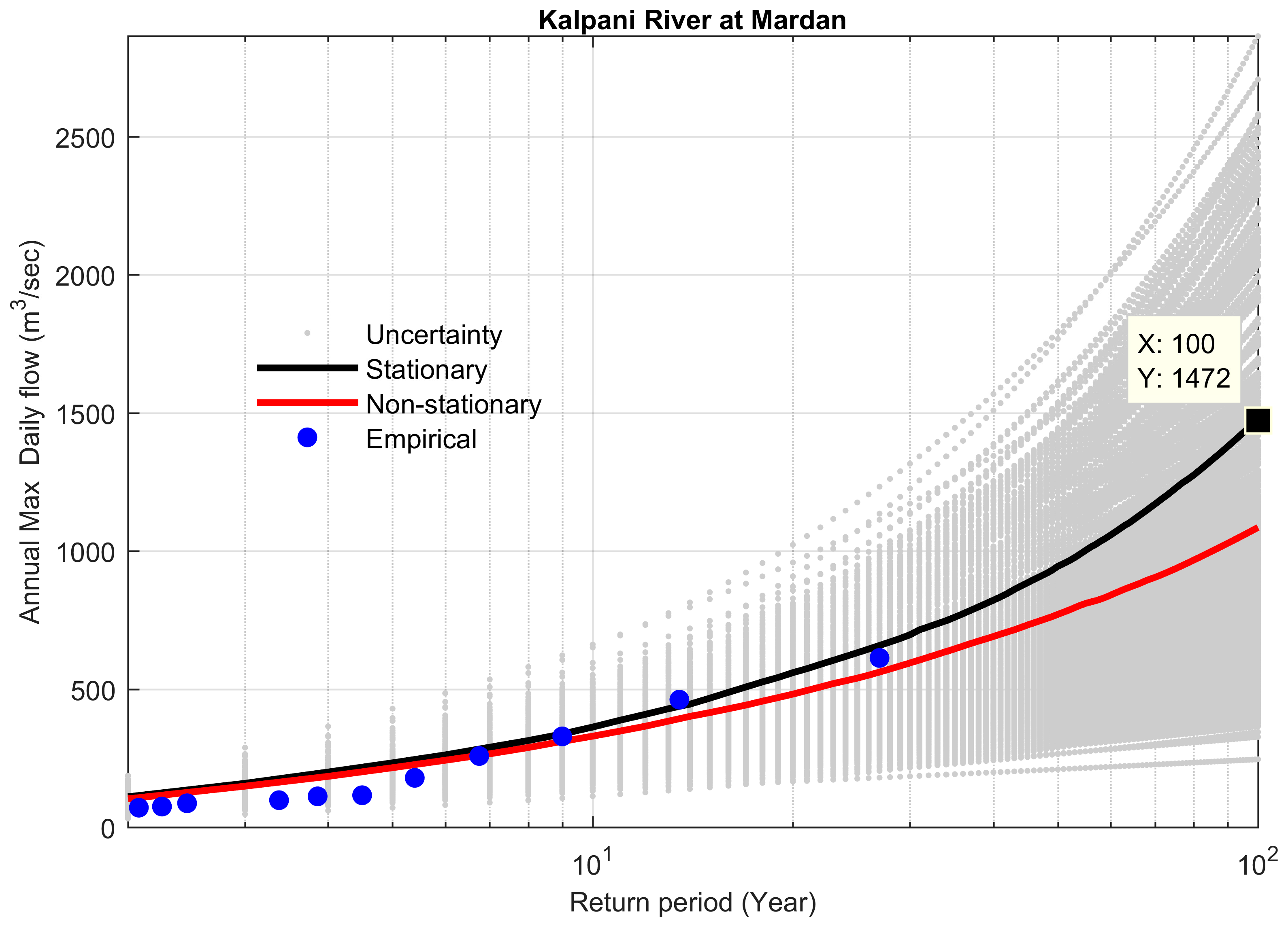
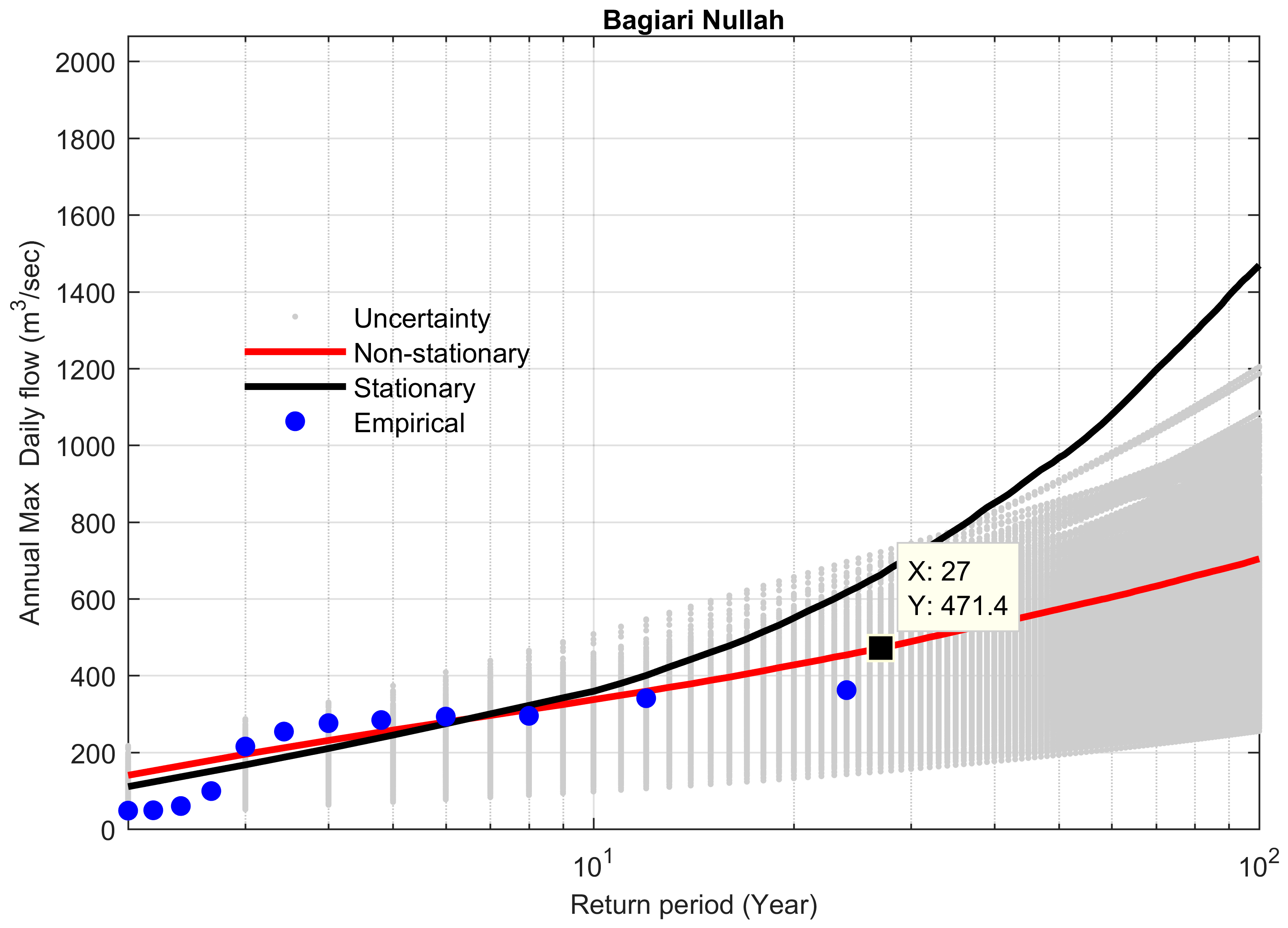
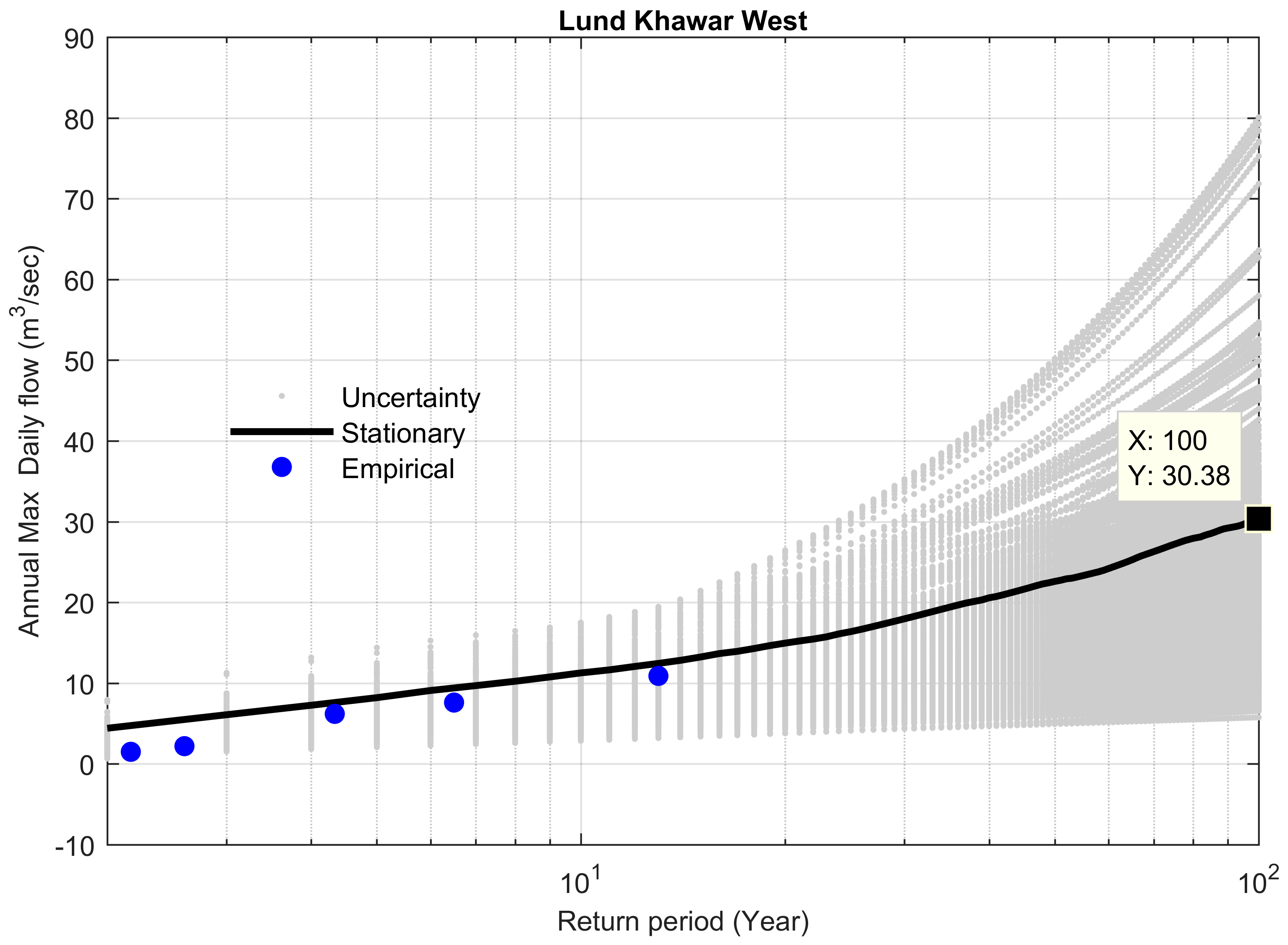
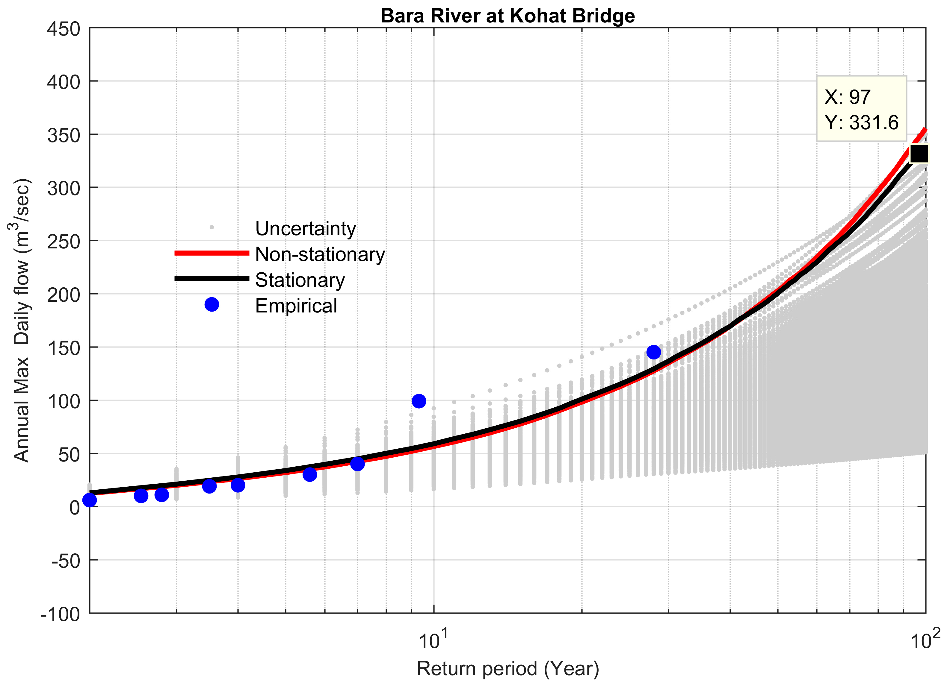
4.4. Comparison between Stationary and Non-Stationary Bayesian Models

Non-stationary FFCs were constructed for the flow gauges with significant increasing trends in their flood series and compared with their stationary FFCs, considering the entire data series without the elimination of outliers.

Table 6. Comparison between 100-year flood estimates using the stationary and non-stationary Bayesian models for “at site modeling” for the KRB, Pakistan.

Site #	Station Name	Historical Extreme m3 s−1	Stationary m3 s−1	Non-Stationary m3 s−1	Difference b/w Stationary & Non-Stationary m3 s−1	Percent Difference (%)	Bayes Factor	% Difference between Preferred Model and Historical Extreme
5	Adezai River	2285	4276	2782	1494	34.9	0.0058	17.86
6	Chitral River	1633	1895	1918	−23	−1.19	0.068	14.85
9	Swat River at Chakdara	1918	1991	2686	−695	−25.8	7.06	3.8
11	Swat River at Ningolai	1475	2891	2528	363	12.5	0.0065	41.65
16	Naranji Nullah	850	1127	1222	−95	−7.7	9.55	24.6
18	Kalpani River at Mardan	1499	3881	2887	1054	27.15	−Infinity	48.14
19	Kalpani River at Risalpur	3358	4918	5140	−222	−4.31	0.4348	34.66
21	Bagiari Nullah	473	1666	819	847	50.8	0.0321	42.24
22	Lund Khawar West	37	76	51	25	32.89	0.11	27.45
24	Bara River at Kohat Bridge	331	686.7	357.5	330.9	48.18	−Infinity	7.2

demonstrates the results at the 95% Bayesian credible interval for all the selected study sites in the KRB. The stationary model showed overestimation as compared to the non-stationary model for a 100-year flood (The flood having a probability of exceedance of 0.01) by 1494 m³ s⁻¹ (+34.9%) for the Adezai River at Adezai Bridge (site 5). The value of the Bayes factor was 0.0058, which was less than 1, so the non-stationary model was favored. The maximum peak flood observed at the Adezai River was 2285 m³ s⁻¹, during the historic flood of 2010 in the KRB. The non-stationary model reasonably described the historical peak flood (Figure 3). Similar behavior was observed for the other study sites, 11, 18, 21, 22, and 24 (Table 6 and Figure 4, Figure 5, Figure 6, Figure 7 and Figure 8).

On the other hand, the stationary model also underestimated the 100-year flood as compared to the non-stationary model. For example, the stationary model underestimated the 100-year flood by 23 m³ s⁻¹ (−1.19%) as compared to the non-stationary model (Figure 9, the Chitral River at Chitral). The value of the Bayes factor was 0.068, which was less than 1, so the non-stationary model was favored. This behavior was obvious for study sites 6 and 19 (Table 6, Figure 9 and Figure 10).

Furthermore, for study sites possessing trends at the significance level of 0.1 (although the trends were modeled at 0.1% for these sites), the non-stationary model overestimated the 100-year flood as compared to the stationary model, and the corresponding value of the Bayes factor was greater than 1. This ultimately favors the stationary model for sites 9 and 16 (Table 6, Figure 11 and Figure 12).

The non-stationary model was found to be reliable for the sites to study the annual maximum flood regime, which exhibits significant trends at α = 0.05. The uncertainty bounds of most of the study sites were high because of the higher value of coefficient of variation, except site 6, where the value of coefficient of variation was 0.2 (see Table 1 and Figure 9). The uncertainty bound could also be higher due to the existence of outliers in the data series. The removal of outliers in the data series can reduce uncertainty.

4.5. Performance of Bayesian Models to Predict the Extreme Floods

The Bayesian models were again re-run for all the study sites before the commencement year of the extreme flood event that we labeled an outlier for all the study sites. Similarly, the objective criterion was adopted again (if a trend exists then modeling was performed using the non-stationary Bayesian model, otherwise only the stationary Bayesian model was used).

Table 7. Performance of Bayesian models for predicting the extreme floods in the KRB, Pakistan.

Site #	Time Series Length	Extreme Event (Year)	Mann–Kendall (Test-Z)	Stationary m3 s−1	Non-Stationary m3 s−1	Difference between Stationary and Non-Stationary m3 s−1	Percent Difference (%)	Bayes Factor
5	1987–2009	2010	−0.05	3300	N/A	N/A	N/A	N/A
6	1964–2004	2005/2010	2.88 **	1701	1978	277	14	0.0054
9	1961–1991	1992	1.42	1746	N/A	N/A	N/A	N/A
11	1986–2015	2016	4.49 ***	2211	1295	916	41.43	15.167
16	1968–2009	2010	1.31	850.8	N/A	N/A	N/A	N/A
18	1984–2009	2010	2.29 *	1472	1085	387	26.3	0.1208
19	1984–2009	2010	2.76 **	4580	3595	990	21.6	0.008
21	1987–2009	2010	2.2 *	1469	704	765	52	0.016
22	1987–1996	1997	−0.28	30.38	N/A	N/A	N/A	N/A
24	1983–2009	2010	1.15	339.6	355	15.4	4.33	+Infinity

*** Trend is significant at α = 0.001, ** Trend is significant at α = 0.01, * Trend is significant at α = 0.05, N/A, Non-stationary Bayesian modeling not applicable because of insignificant or no trend.

describes the results of the corresponding stationary and non-stationary Bayesian models.

The Bayesian models performed well, predicting the extreme floods satisfactorily for all the study sites except sites 9 and 22 (see Table 7 and Figure 13, Figure 14, Figure 15, Figure 16, Figure 17, Figure 18, Figure 19, Figure 20, Figure 21 and Figure 22). The stationary Bayesian model was found reliable for sites 5, 6, 11, 16, 21, and 24. However, the non-stationary model was favored as compared to the stationary model as per the Bayes factor criterion (see Table 7) for sites 6, 18, 19, and 21. Despite the existence of a significant trend at site 11, the stationary model was favored as per the Bayes factor criterion, as well as predicting the extreme flood of 2016.

The outlier’s removal improved the fitting of the FFCs as compared to considering the entire data series and also reduced the uncertainty (see Figure 13, Figure 14, Figure 15, Figure 16, Figure 17, Figure 18, Figure 19, Figure 20, Figure 21 and Figure 22).

Statistical modeling of extremes in hydrology is exciting and challenging, and opens the door for further studies. For example, for study site 9 (the Swat River at Chakdara), it is better to consider the entire data series, and for better fitting, the incorporation of monsoon rainfall as a covariate might be fruitful. The modeling could also be performed by considering other distributions in the Bayesian framework or using the traditional frequentist framework.

Finally, from a regional perspective, the region is heterogeneous due to large altitudinal variations. Due to the regional heterogeneity associated with elevation, it seems to be quite difficult to develop a regional Bayesian model for the whole KRB, but efforts should be made to develop a regional Bayesian model at sub-basin or catchment scales in future studies by further pooling of information for other parameters, like location and scale, across sites. Moreover, the studies are also required to deeply understand the impact of climate or dominating weather patterns, such as the South Asian monsoon, low climate variability El-Niño Southern Oscillation and Indian Ocean Dipole (ENSO, IOD, etc.) and human factors, such as land use cover change (LUCC), population increase, and reservoir construction, on the flood regime of the KRB [1,13,80,81,82,83].

5. Conclusions

Analyzing the flood regime and its non-stationary modeling in a Bayesian framework for the KRB was the main objective of the present study. To achieve this, a Mann–Kendall trend analysis was performed to explore the flood regime of the KRB in detail, and finally, the stationary and non-stationary Bayesian models with informed priors on shape parameter for GEV distribution were developed, and their results were compared by using the corresponding FFCs, along with their uncertainty bounds. We utilized the annual extreme data of flood series for the study area, with a maximum record of 1962–2016 (55 years) and a minimum of 1987–2016 (30 years). The key findings of the study are described below:

• Trend analysis showed a mixture of increasing and decreasing trends at different gauges in the KRB at α = 0.05. The Chitral River, Kalpani River, Main Swat River, and Bara River basins showed significant increasing trends, and the Panjkora River basin displayed a moderate increasing trend in its annual maximum flood regime. However, the Lower Swat and Kabul sub-basins showed decreasing trends, except for the Adezai River in the Kabul sub-basin, which showed a significant increasing trend.
• The overall basin was under critical change and signals of clear non-stationarity in the flood regime were evident at various spatial scales throughout the basin.
• The presence of a significant trend and significant difference in flood estimates for 100-year flood between stationary and non-stationary FFCs were found that represent the clear violation from the so-called stationary assumption.
• The non-stationary Bayesian model was found to be reliable for the study sites that had a significant trend at α = 0.05, while the stationary model overestimated or underestimated the flood risk for these sites. On the other hand, the stationary Bayesian model performed better for the study sites for trends at α = 0.1, while the non-stationary Bayesian model overestimated or underestimated the flood risk for such sites.
• The use of informed priors on the shape parameter based on regional information improved the estimation of flood quantiles and reduced the uncertainty.
• Proper consideration should be given to identify the outliers while using Bayesian models.
• The presence of non-stationarity in the flood regime of the KRB has substantial implications for flood management and water resources development. A design with stationary assumption will cause two major concerns: under estimation or overestimation of design for structural and non-structural measures in the KRB. An event-based design may also overestimate or underestimate the risk in hydraulic design that was intended. Some previous studies in other parts of world also provided similar results [1,13,31,84,85,86].

The study will be helpful for sustainable flood management and provide a reference for studying floods in a changing environment for hydrologists, water resources managers, decision makers, and concerned organizations.

References

1. López, J.; Francés, F. Non-stationary flood frequency analysis in continental Spanish rivers, using climate and reservoir indices as external covariates. Hydrol. Earth Syst. Sci. 2013, 17, 3189–3203. [Google Scholar] [CrossRef] [Green Version]
2. Khaliq, M.; Ouarda, T.; Ondo, J.-C.; Gachon, P.; Bobée, B. Frequency analysis of a sequence of dependent and/or non-stationary hydro-meteorological observations: A review. J. Hydrol. 2006, 329, 534–552. [Google Scholar] [CrossRef]
3. Stedinger, J.R.; Vogel, R.; Foufoula-Georgiou, E. Frequency analysis of extreme events. Handb. Hydrol. 1993, 18, 68. [Google Scholar]
4. Salas, J. Analysis and Modeling of Hydrologic Time Series in Hand Book of Hydrology; Maidment, D.R., Ed.; McGraw Hill Book Co.: New York, NY, USA, 1993. [Google Scholar]
5. Council, N.R. Decade-to-Century-Scale Climate Variability and Change: A Science Strategy; National Academies Press: Washington, DC, USA, 1998. [Google Scholar]
6. Norrant, C.; Douguédroit, A. Monthly and daily precipitation trends in the Mediterranean (1950–2000). Theor. Appl. Climatol. 2006, 83, 89–106. [Google Scholar] [CrossRef]
7. Mudelsee, M.; Börngen, M.; Tetzlaff, G.; Grünewald, U. No upward trends in the occurrence of extreme floods in central Europe. Nature 2003, 425, 166–169. [Google Scholar] [CrossRef]
8. Douglas, E.; Vogel, R.; Kroll, C. Trends in floods and low flows in the United States: Impact of spatial correlation. J. Hydrol. 2000, 240, 90–105. [Google Scholar] [CrossRef]
9. Franks, S.W. Identification of a change in climate state using regional flood data. Hydrol. Earth Syst. Sci. 2002, 6, 11–16. [Google Scholar] [CrossRef]
10. Milly, P.C.; Dunne, K.A.; Vecchia, A.V. Global pattern of trends in streamflow and water availability in a changing climate. Nature 2005, 438, 347–350. [Google Scholar] [CrossRef]
11. Villarini, G.; Serinaldi, F.; Smith, J.A.; Krajewski, W.F. On the stationarity of annual flood peaks in the continental united states during the 20th century. Water Resour. Res. 2009, 45. [Google Scholar] [CrossRef]
12. Wilson, D.; Hisdal, H.; Lawrence, D. Has streamflow changed in the nordic countries?–recent trends and comparisons to hydrological projections. J. Hydrol. 2010, 394, 334–346. [Google Scholar] [CrossRef]
13. Villarini, G.; Smith, J.A.; Serinaldi, F.; Bales, J.; Bates, P.D.; Krajewski, W.F. Flood frequency analysis for nonstationary annual peak records in an urban drainage basin. Adv. Water Resour. 2009, 32, 1255–1266. [Google Scholar] [CrossRef]
14. Vogel, R.M.; Yaindl, C.; Walter, M. Nonstationarity: Flood magnification and recurrence reduction factors in the United States. J. Am. Water Resour. Assoc. 2011, 47, 464–474. [Google Scholar] [CrossRef]
15. Hejazi, M.I.; Markus, M. Impacts of urbanization and climate variability on floods in northeastern Illinois. J. Hydrol. Eng. 2009, 14, 606–616. [Google Scholar] [CrossRef]
16. Held, I.M.; Soden, B.J. Robust responses of the hydrological cycle to global warming. J. Clim. 2006, 19, 5686–5699. [Google Scholar] [CrossRef]
17. Allen, M.R.; Smith, L.A. Monte carlo ssa: Detecting irregular oscillations in the presence of colored noise. J. Clim. 1996, 9, 3373–3404. [Google Scholar] [CrossRef]
18. Zaman, C.Q.U.; Mahmood, A.; Rasul, G.; Afzal, M. Climate Change Indicators of Pakistan; Report No: PMD-22/2009; Pakistan Meteorological Department: Islamabad, Pakistan, 2009.
19. Ahmad, I.; Tang, D.; Wang, T.; Wang, M.; Wagan, B. Precipitation trends over time using mann-kendall and spearman’s rho tests in Swat river basin, Pakistan. Adv. Meteorol. 2015, 2015, 431860. [Google Scholar] [CrossRef]
20. Khalid, S.; Rehman, S.U.; Shah, S.M.A.; Naz, A.; Saeed, B.; Alam, S.; Ali, F.; Gul, H. Hydro-meteorological characteristics of Chitral river basin at the peak of the Hindukush range. Nat. Sci. 2013, 5, 987. [Google Scholar] [CrossRef]
21. Hartmann, H.; Buchanan, H. Trends in extreme precipitation events in the Indus river basin and flooding in Pakistan. Atmos. Ocean 2014, 52, 77–91. [Google Scholar] [CrossRef]
22. Najmuddin, O.; Deng, X.; Siqi, J. Scenario analysis of land use change in Kabul river basin–a river basin with rapid socio-economic changes in Afghanistan. Phys. Chem. Earth Parts A B C 2017, 101, 121–136. [Google Scholar] [CrossRef]
23. Qasim, M.; Hubacek, K.; Termansen, M.; Khan, A. Spatial and temporal dynamics of land use pattern in district Swat, Hindu Kush Himalayan region of Pakistan. Appl. Geogr. 2011, 31, 820–828. [Google Scholar] [CrossRef]
24. Ullah, S.; Farooq, M.; Shafique, M.; Siyab, M.A.; Kareem, F.; Dees, M. Spatial assessment of forest cover and land-use changes in the Hindu-Kush mountain ranges of northern Pakistan. J. Mt. Sci. 2016, 13, 1229–1237. [Google Scholar] [CrossRef]
25. Sajjad, A.; Adnan, S.; Hussain, A. Forest land cover change from year 2000 to 2012 of tehsil Barawal Dir Upper Pakistan. Int. J. Adv. Res. Biol. Sci. 2016, 3, 144–154. [Google Scholar]
26. Ahmad, A.; Nizami, S.M. Carbon stocks of different land uses in the Kumrat valley, Hindu Kush region of Pakistan. J. For. Res. 2015, 26, 57–64. [Google Scholar] [CrossRef]
27. Yar, P.; Atta-ur-Rahman, M.A.K.; Samiullah, S. Spatio-temporal analysis of urban expansion on farmland and its impact on the agricultural land use of Mardan city, Pakistan. Proc. Pak. Acad. Sci. B Life Environ. Sci. 2016, 53, 35–46. [Google Scholar]
28. Raziq, A.; Xu, A.; Li, Y.; Zhao, Q. Monitoring of land use/land cover changes and urban sprawl in peshawar city in khyber pakhtunkhwa: An application of geo-information techniques using of multi-temporal satellite data. J. Remote Sens. GIS 2016, 5. [Google Scholar] [CrossRef]
29. Milly, P.C.; Betancourt, J.; Falkenmark, M.; Hirsch, R.M.; Kundzewicz, Z.W.; Lettenmaier, D.P.; Stouffer, R.J. Stationarity is dead: Whither water management? Science 2008, 319, 573–574. [Google Scholar] [CrossRef] [PubMed]
30. Delgado, J.M.; Apel, H.; Merz, B. Flood trends and variability in the Mekong river. Hydrol. Earth Syst. Sci. 2010, 14, 407–418. [Google Scholar] [CrossRef] [Green Version]
31. Leclerc, M.; Ouarda, T.B. Non-stationary regional flood frequency analysis at ungauged sites. J. Hydrol. 2007, 343, 254–265. [Google Scholar] [CrossRef]
32. Olsen, J.R.; Lambert, J.H.; Haimes, Y.Y. Risk of extreme events under nonstationary conditions. Risk Anal. 1998, 18, 497–510. [Google Scholar] [CrossRef]
33. McNeil, A.J.; Saladin, T. Developing Scenarios for Future Extreme Losses Using the Pot Method. In Extremes and Integrated Risk Management; Embrechts, P., Ed.; CiteseerX: Zurich, Switzerland, 2000; pp. 253–267. [Google Scholar]
34. Stedinger, J.R.; Crainiceanu, C.M. Climate Variability and Flood-Risk Management. In Risk-Based Decision Making in Water Resources IX; ASCE: Reston, VA, USA, 2001; pp. 77–86. [Google Scholar]
35. Strupczewski, W.; Singh, V.; Mitosek, H. Non-stationary approach to at-site flood frequency modelling. III. Flood analysis of Polish rivers. J. Hydrol. 2001, 248, 152–167. [Google Scholar] [CrossRef]
36. He, Y.; Bárdossy, A.; Brommundt, J. Non-Stationary Flood Frequency Analysis in Southern Germany. In Proceedings of the Seventh International Conference on Hydroscience and Engineering, Philadelphia, PA, USA, 10–13 September 2006. [Google Scholar]
37. Renard, B.; Lang, M.; Bois, P. Statistical analysis of extreme events in a non-stationary context via a bayesian framework: Case study with peak-over-threshold data. Stoch. Environ. Res. Risk Assess. 2006, 21, 97–112. [Google Scholar] [CrossRef]
38. Khattak, M.; Anwar, F.; Sheraz, K.; Saeed, T.; Sharif, M.; Ahmed, A. Floodplain mapping using hec-ras and arcgis: A case study of Kabul river. Arab. J. Sci. Eng. (Springer Sci. Bus. Media BV) 2016, 41, 1375–1390. [Google Scholar] [CrossRef]
39. Sayama, T.; Ozawa, G.; Kawakami, T.; Nabesaka, S.; Fukami, K. Rainfall–runoff–inundation analysis of the 2010 Pakistan flood in the Kabul river basin. Hydrol. Sci. J. 2012, 57, 298–312. [Google Scholar] [CrossRef]
40. Bahadar, I.; Shafique, M.; Khan, T.; Tabassum, I.; Ali, M.Z. Flood hazard assessment using hydro-dynamic model and gis/rs tools: A case study of Babuzai-Kabal tehsil Swat basin, Pakistan. J. Himal. Earth Sci. 2015, 48, 129–138. [Google Scholar]
41. Aziz, A. Rainfall-runoff modeling of the trans-boundary Kabul river basin using integrated flood analysis system (ifas). Pak. J. Meteorol. 2014, 10, 75–81. [Google Scholar]
42. Ullah, S.; Farooq, M.; Sarwar, T.; Tareen, M.J.; Wahid, M.A. Flood modeling and simulations using hydrodynamic model and aster dem—A case study of Kalpani river. Arab. J. Geosci. 2016, 9, 439. [Google Scholar] [CrossRef]
43. Mack, T.J.; Chornack, M.P.; Taher, M.R. Groundwater-level trends and implications for sustainable water use in the Kabul basin, afghanistan. Environ. Syst. Decis. 2013, 33, 457–467. [Google Scholar] [CrossRef]
44. Lashkaripour, G.R.; Hussaini, S. Water resource management in Kabul river basin, Eastern Afghanistan. Environmentalist 2008, 28, 253–260. [Google Scholar] [CrossRef]
45. Tariq, M.A.U.R.; Van de Giesen, N. Floods and flood management in Pakistan. Phys. Chem. Earth Parts A B C 2012, 47, 11–20. [Google Scholar] [CrossRef]
46. Anjum, M.N.; Ding, Y.; Shangguan, D.; Ijaz, M.W.; Zhang, S. Evaluation of high-resolution satellite-based real-time and post-real-time precipitation estimates during 2010 extreme flood event in Swat river basin, Hindukush region. Adv. Meteorol. 2016, 2016, 2604980. [Google Scholar] [CrossRef]
47. Rasul, G.; Dahe, Q.; Chaudhry, Q. Global warming and melting glaciers along southern slopes of HKH range. Pak. J. Meteorol. 2008, 5, 63–76. [Google Scholar]
48. Mann, H.B. Nonparametric tests against trend. Econom. J. Econom. Soc. 1945, 13, 245–259. [Google Scholar] [CrossRef]
49. Kendall, M. Rank Correlation Methods; Charles Griffin: London, UK, 1975. [Google Scholar]
50. Katz, R.W. Statistics of extremes in climate change. Clim. Chang. 2010, 100, 71–76. [Google Scholar] [CrossRef]
51. Coles, S.; Bawa, J.; Trenner, L.; Dorazio, P. An Introduction to Statistical Modeling of Extreme Values; Springer: Berlin/Heidelberg, Germany, 2001; Volume 208. [Google Scholar]
52. Smith, R. Extreme value statistics in meteorology and the environment. Environ. Stat. 2001, 8, 300–357. [Google Scholar]
53. Shukla, R.K.; Trivedi, M.; Kumar, M. On the proficient use of gev distribution: A case study of subtropical monsoon region in India. arXiv 2012, arXiv:1203.0642. [Google Scholar]
54. Massey, F.J., Jr. The kolmogorov-Smirnov test for goodness of fit. J. Am. Stat. Assoc. 1951, 46, 68–78. [Google Scholar] [CrossRef]
55. Mehrannia, H.; Pakgohar, A. Using easy fit software for goodness-of-fit test and data generation. Int. J. Math. Arch. 2014, 5, 118–124. [Google Scholar]
56. Lin, L.; Sherman, P.D. Cleaning Data the Chauvenet Way. In Proceedings of the SouthEast SAS Users Group, Hilton Head Island, SC, USA, 4–6 November 2007. SESUG Proceedings, Paper SA11. [Google Scholar]
57. Renard, B.; Sun, X.; Lang, M. Bayesian Methods for Non-Stationary Extreme Value Analysis. In Extremes in a Changing Climate; Springer: Berlin/Heidelberg, Germany, 2013; pp. 39–95. [Google Scholar]
58. Meehl, G.A.; Karl, T.; Easterling, D.R.; Changnon, S.; Pielke, R., Jr.; Changnon, D.; Evans, J.; Groisman, P.Y.; Knutson, T.R.; Kunkel, K.E. An introduction to trends in extreme weather and climate events: Observations, socioeconomic impacts, terrestrial ecological impacts, and model projections. Bull. Am. Meteorol. Soc. 2000, 81, 413–416. [Google Scholar] [CrossRef]
59. Gilleland, E.; Katz, R.W. New software to analyze how extremes change over time. Eos Trans. Am. Geophys. Union 2011, 92, 13–14. [Google Scholar] [CrossRef]
60. Cheng, L.; AghaKouchak, A.; Gilleland, E.; Katz, R.W. Non-stationary extreme value analysis in a changing climate. Clim. Chang. 2014, 127, 353–369. [Google Scholar] [CrossRef]
61. Stephenson, A.; Tawn, J. Bayesian inference for extremes: Accounting for the three extremal types. Extremes 2004, 7, 291–307. [Google Scholar] [CrossRef]
62. Ragno, E.; AghaKouchak, A.; Love, C.A.; Cheng, L.; Vahedifard, F.; Lima, C.H. Quantifying changes in future intensity-duration-frequency curves using multimodel ensemble simulations. Water Resour. Res. 2018, 54, 1751–1764. [Google Scholar] [CrossRef]
63. Martins, E.S.; Stedinger, J.R. Generalized maximum-likelihood generalized extreme-value quantile estimators for hydrologic data. Water Resour. Res. 2000, 36, 737–744. [Google Scholar] [CrossRef]
64. Ter Braak, C.J. A Markov chain monte carlo version of the genetic algorithm differential evolution: Easy bayesian computing for real parameter spaces. Stat. Comput. 2006, 16, 239–249. [Google Scholar] [CrossRef]
65. Vrugt, J.A.; Ter Braak, C.; Diks, C.; Robinson, B.A.; Hyman, J.M.; Higdon, D. Accelerating markov chain monte carlo simulation by differential evolution with self-adaptive randomized subspace sampling. Int. J. Nonlinear Sci. Numer. Simul. 2009, 10, 273–290. [Google Scholar] [CrossRef]
66. Gelman, A.; Shirley, K. Inference from Simulations and Monitoring Convergence. In Handbook. Markov Chain Monte Carlo; CRC Press: Boca Raton, FA, USA, 2011; pp. 163–174. [Google Scholar]
67. Kass, R. Re kass and ae raftery. J. Am. Stat. Assoc. 1995, 90, 773–795. [Google Scholar] [CrossRef]
68. Khan, A. Analysis of streamflow data for trend detection on major rivers of the indus basin. J. Himal. Earth Sci. Vol. 2015, 48, 99–111. [Google Scholar]
69. Khan, K.; Yaseen, M.; Latif, Y.; Nabi, G. Detection of river flow trends and variability analysis of Upper Indus basin, pakistan. Sci. Int. 2015, 27, 1261–1270. [Google Scholar]
70. Sharif, M.; Archer, D.; Fowler, H.; Forsythe, N. Trends in timing and magnitude of flow in the Upper Indus basin. Hydrol. Earth Syst. Sci. 2013, 17, 1503–1516. [Google Scholar] [CrossRef]
71. Rosner, A.; Vogel, R.M.; Kirshen, P.H. A risk-based approach to flood management decisions in a nonstationary world. Water Resour. Res. 2014, 50, 1928–1942. [Google Scholar] [CrossRef]
72. Sun, X.; Thyer, M.; Renard, B.; Lang, M. A general regional frequency analysis framework for quantifying local-scale climate effects: A case study of enso effects on southeast Queensland rainfall. J. Hydrol. 2014, 512, 53–68. [Google Scholar] [CrossRef]
73. Halbert, K.; Nguyen, C.C.; Payrastre, O.; Gaume, E. Reducing uncertainty in flood frequency analyses: A comparison of local and regional approaches involving information on extreme historical floods. J. Hydrol. 2016, 541, 90–98. [Google Scholar] [CrossRef]
74. Kyselý, J.; Gaál, L.; Picek, J. Comparison of regional and at-site approaches to modelling probabilities of heavy precipitation. Int. J. Climatol. 2011, 31, 1457–1472. [Google Scholar] [CrossRef]
75. Viglione, A.; Merz, R.; Salinas, J.L.; Blöschl, G. Flood frequency hydrology: 3. A bayesian analysis. Water Resour. Res. 2013, 49, 675–692. [Google Scholar] [CrossRef]
76. Kuczera, G. Combining site-specific and regional information: An empirical bayes approach. Water Resour. Res. 1982, 18, 306–314. [Google Scholar] [CrossRef]
77. Sun, X.; Lall, U.; Merz, B.; Dung, N.V. Hierarchical bayesian clustering for nonstationary flood frequency analysis: Application to trends of annual maximum flow in Germany. Water Resour. Res. 2015, 51, 6586–6601. [Google Scholar] [CrossRef]
78. Katz, R.W.; Parlange, M.B.; Naveau, P. Statistics of extremes in hydrology. Adv Water Resour. 2002, 25, 1287–1304. [Google Scholar] [CrossRef] [Green Version]
79. Lima, C.H.; Lall, U.; Troy, T.; Devineni, N. A hierarchical bayesian gev model for improving local and regional flood quantile estimates. J. Hydrol. 2016, 541, 816–823. [Google Scholar] [CrossRef]
80. Kwon, H.H.; Brown, C.; Lall, U. Climate informed flood frequency analysis and prediction in Montana using hierarchical bayesian modeling. Geophys. Res. Lett. 2008, 35. [Google Scholar] [CrossRef]
81. Steinschneider, S.; Lall, U. A hierarchical bayesian regional model for nonstationary precipitation extremes in northern california conditioned on tropical moisture exports. Water Resour. Res. 2015, 51, 1472–1492. [Google Scholar] [CrossRef]
82. Lima, C.H.; Lall, U.; Troy, T.J.; Devineni, N. A climate informed model for nonstationary flood risk prediction: Application to negro river at Manaus, Amazonia. J. Hydrol. 2015, 522, 594–602. [Google Scholar] [CrossRef]
83. Machado, M.J.; Botero, B.; López, J.; Francés, F.; Díez-Herrero, A.; Benito, G. Flood frequency analysis of historical flood data under stationary and non-stationary modelling. Hydrol. Earth Syst. Sci. 2015, 19, 2561–2576. [Google Scholar] [CrossRef] [Green Version]
84. Šraj, M.; Viglione, A.; Parajka, J.; Blöschl, G. The influence of non-stationarity in extreme hydrological events on flood frequency estimation. J. Hydrol. Hydromech. 2016, 64, 426–437. [Google Scholar] [CrossRef] [Green Version]
85. Hounkpè, J.; Diekkrüger, B.; Badou, D.F.; Afouda, A.A. Non-stationary flood frequency analysis in the Ouémé river basin, Benin Republic. Hydrology 2015, 2, 210–229. [Google Scholar] [CrossRef]
86. Xiong, L.; Du, T.; Xu, C.-Y.; Guo, S.; Jiang, C.; Gippel, C.J. Non-stationary annual maximum flood frequency analysis using the norming constants method to consider non-stationarity in the annual daily flow series. Water Resour. Manag. 2015, 29, 3615–3633. [Google Scholar] [CrossRef]
Figure 1. Description of Location, SRTM-DEM (Shuttle Radar Topography Mission–digital elevation model, meters) and flow gauge stations for the Kabul River basin (KRB), Pakistan.
Water 11 01246 g001
Figure 2. Spatial distribution of trends in the annual maximum flood regime of the KRB, Pakistan.
Water 11 01246 g002
Figure 3. Comparison between non-stationary and stationary flood frequency curves (FFCs) at site 5, along with non-stationary uncertainty bounds for the year 2016.
Water 11 01246 g003
Figure 4. Comparison between non-stationary and stationary FFCs at site 11, along with non-stationary uncertainty bounds for the year 2016.
Water 11 01246 g004
Figure 5. Comparison between non-stationary and stationary FFCs at site 18, along with non-stationary uncertainty bounds for the year 2016.
Water 11 01246 g005
Figure 6. Comparison between non-stationary and stationary FFCs at site 21, along with non-stationary uncertainty bounds for the year 2016.
Water 11 01246 g006
Figure 7. Comparison between non-stationary and stationary FFCs at site 22, along with non-stationary uncertainty bounds for the year 2016.
Water 11 01246 g007
Figure 8. Comparison between non-stationary and stationary FFCs at site 24, along with non-stationary uncertainty bounds for the year 2016.
Water 11 01246 g008
Figure 9. Comparison between non-stationary and stationary FFCs at site 6, along with non-stationary uncertainty bounds for the year 2013.
Water 11 01246 g009
Figure 10. Comparison between non-stationary and stationary FFCs at site 19, along with non-stationary uncertainty bounds for the year 2016.
Water 11 01246 g010
Figure 11. Comparison between non-stationary and stationary FFCs at site 9, along with non-stationary uncertainty bounds for the year 2009.
Water 11 01246 g011
Figure 12. Comparison between non-stationary and stationary FFCs at site 16, along with non-stationary uncertainty bounds for the year 2016.
Water 11 01246 g012
Figure 13. FFCs at site 5, along with stationary uncertainty bounds for the year 2009.
Water 11 01246 g013
Figure 14. Comparison between non-stationary and stationary FFCs at site 6, along with non-stationary uncertainty bounds for the year 2004.
Water 11 01246 g014
Figure 15. FFCs at site 9, along with stationary uncertainty bounds for the year 1991.
Water 11 01246 g015
Figure 16. Comparison between non-stationary and stationary FFCs at site 11, along with non-stationary uncertainty bounds for the year 2015.
Water 11 01246 g016
Figure 17. FFCs at site 16, along with stationary uncertainty bounds for the year 2009.
Water 11 01246 g017
Figure 18. Comparison between non-stationary and stationary FFCs at site 18, along with non-stationary uncertainty bounds for the year 2009.
Water 11 01246 g018
Figure 19. Comparison between non-stationary and stationary FFCs at site 19, along with non-stationary uncertainty bounds for the year 2009.
Water 11 01246 g019
Figure 20. Comparison between non-stationary and stationary FFCs at site 21, along with non-stationary uncertainty bounds for the year 2009.
Water 11 01246 g020
Figure 21. FFCs at site 22, along with stationary uncertainty bounds for the year 1996.
Water 11 01246 g021
Figure 22. Comparison between non-stationary and stationary FFCs at site 24, along with non-stationary uncertainty bounds for the year 2009.
Water 11 01246 g022