Article

Groundwater Nitrate Contamination Integrated Modeling for Climate and Water Resources Scenarios: The Case of Lake Karla Over-Exploited Aquifer

by
Pantelis Sidiropoulos
1,*,
Georgios Tziatzios
1,
Lampros Vasiliades
1,
Nikitas Mylopoulos
1 and
Athanasios Loukas
1,2
1
Laboratory of Hydrology and Aquatic Systems Analysis, Department of Civil Engineering, School of Engineering, University of Thessaly, Volos 38334, Greece
2
Department of Rural and Surveying Engineering, Aristotle University of Thessaloniki, Thessaloniki 54124, Greece
*
Author to whom correspondence should be addressed.
Water 2019, 11(6), 1201; https://doi.org/10.3390/w11061201
Submission received: 17 January 2019 / Revised: 14 March 2019 / Accepted: 4 June 2019 / Published: 8 June 2019
(This article belongs to the Section Water, Agriculture and Aquaculture)

Abstract

:
Groundwater quantity and quality degradation by agricultural practices is recorded as one of the most critical issues worldwide. This is explained by the fact that groundwater is an important component of the hydrological cycle, since it is a source of natural enrichment for rivers, lakes, and wetlands and constitutes the main source of potable water. The need of aquifers simulation, taking into account water resources components at watershed level, is imperative for the choice of appropriate restoration management practices. An integrated water resources modeling approach, using hydrological modeling tools, is presented for assessing the nitrate fate and transport on an over-exploited aquifer with intensive and extensive agricultural activity under various operational strategies and future climate change scenarios. The results indicate that climate change affects nitrates concentration in groundwater, which is likely to be increased due to the depletion of the groundwater table and the decrease of groundwater enrichment in the future water balance. Application of operational agricultural management practices with the construction and use of water storage infrastructure tend to compensate the groundwater resources degradation due to climate change impacts.

Graphical Abstract

1. Introduction

The development of modeling in surface and ground water hydrology is based on the causative relationships among the hydrological cycle, climate, geomorphology, hydrogeology, and human activities interaction on the above components [1]. According to Biswas [2], the complexity and particularity of integrated water resources management is attributed to 24 different issues which are included in integrated water resources management. One of the 24 issues is the coupling of surface water and groundwater modeling. The difficulty of an integrated approach of these two water resources components modeling for different temporal and spatial scales is mentioned by many scientists in literature. The dynamic processes of surface and groundwater systems are mainly influenced by the hydrological and hydrogeological conditions for integrated water resources management at watershed level [3]. Therefore, understanding surface and groundwater processes requires the understanding of the impact of geomorphology, hydrogeology, and climate on subsurface flow systems [4]. An integrated approach leads to conclusions related to how recharge and discharge are influenced under climate scenarios and management strategies [5]. Moreover, surface water–groundwater interactions could provide important information for contaminated areas [6].
High concentration values of nitrates in the saturated zone is recognized as a serious threat to groundwater quality as indicated by several studies [7,8,9,10,11,12,13,14,15,16,17,18]. Groundwater contamination is classified in two main categories—non-point and point sources. Nitrate in groundwater may be derived from industrial, municipal, residential, and agricultural sources. Several studies show a significant correlation between agriculture and increased nitrate concentration in groundwater [7,15,16]. Non-point agriculture sources include nitrogen fertilizers, manure application, leguminous crops, irrigation return-flows, dissolved nitrogen in precipitation, and dry deposition [19,20]. Groundwater nitrate contamination is considered as a major concern in rural areas, where agriculture is the main human occupation and economic activity and arises as a result of increased water demands as well as increased application of nitrogen fertilizers [21,22]. Nitrogen is led to the saturated zone mainly in the form of nitrate due to the denitrification process which occurs in the vadose zone [15]. Almasri and Kaluarachchi [23] characterize nitrate anions ( NO 3 ) as the most commonly encountered inorganic pollutant in groundwater resources of rural watersheds, owing to their negative electrical load and the low sorption ability of soils, and most importantly to their high mobility and water solubility. Nitrate anions are dissolved in soil water and lost through the water movement in two ways: The direct way, where leaching is performed at the vertical movement of dissolved molecules of nitrogen through the soil profile to the saturated zone; and the indirect way, where the surface runoff solutes are moving over the ground surface until they reach open channels such as field drains, rivers, or lakes [12,24]. Extensive agricultural land use is related to subsurface nitrate contamination that has been linked to adverse health concerns [21,22,25]. There are two types of farming systems—the intensive cropping system and the extensive one. The intensive consists of the arable crops which predominate in Mediterranean areas [26]. The leading forces of utilizing nitrogen-based fertilizers in agriculture is the globally increasing demand for food, the improvement of the crop yield as well as the quality of products. This is primarily caused by a growing world population with a high demand for food production and food quality [27]. Groundwater contamination possibly leads to social and economic losses which may be also influenced by climate change, crop pattern, and crop management [28].
Agriculture activity is closely linked to both ecosystems and society under a two-way relationship: it is obviously affected by environmental changes and, at the same time, its practices directly affect the environment. Climate change is a continuously variable global phenomenon effecting various factors including water quantity and quality assessment as well as surface water and groundwater systems management [29,30]. Human activities in ground and water resources management are, in turn, in close relationship with climate scenarios, especially within the Mediterranean region, an area recognized as one of the world’s most affected by climate change. Local climatic simulation models estimate a significant decrease in precipitation and higher temperatures in the region for the forthcoming period [31]. Furthermore, climate variability and climate change reveal negative impacts in the hydrogeological environment with the decreased recharge rates and the increased water withdrawals affecting the renewable groundwater resources. Impacts on the saturated zone could also be attributed to human activities due to different land use and crop management practices [32,
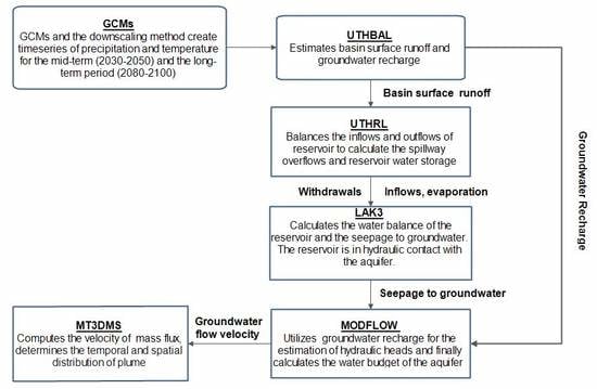
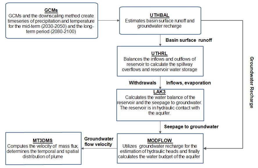
33]. Therefore, the determination of climate change consequences on groundwater systems requires future assessment of the hydrological variables that interact directly with the hydrogeological environment (e.g., groundwater recharge, pumping, pollutant leaching, etc.). The assessment of future conditions impacts (climate, land use, water demands, etc.) on groundwater systems, is achieved with the coupling of mathematical models which represents hydrological and hydrogeological processes [30]. In this study, surface-groundwater integrated modeling is applied in order to investigate the impact of climate change scenarios and the effects of different operational water resources management strategies on groundwater quantity and quality at Lake Karla watershed, Thessaly, Greece. The paper emphasizes groundwater quality investigation and particularly emphasizes the simulation of advection and dispersion of nitrate mass of the Lake Karla aquifer.

2. Materials and Methods

2.1. Study Area Description

Lake Karla watershed is located at the southeastern part of the Thessaly plain, Greece, and has an area of 1171 km2 (Figure 1). Agriculture is the main economic activity and as a result is the major source of income of the local population. The study area is included in the main agricultural region of Greece (i.e., Thessaly) and it is extensively cultivated with crops characterized by increased water and fertilization demands such as maize, cotton, and alfalfa [34]. According to Directive 91/676/EEC, the Thessaly plain area and especially Lake Karla watershed has been identified as Nitrate Vulnerable Zones (NVZs) from agricultural practices. Figure 2 shows the major land use categories and the spatial distribution of crop pattern for the year 2001, whereas Table 1 presents the Land Use and Crop Classification percentage areas and show that the arable cropping systems (cotton, wheat, maize, cereals etc.) dominate in the study area and cover 335.51 km2 or 67.10% of the total aquifer area.

2.2. Climate, Hydrology, and Climate Change Scenarios

The climate of Lake Karla watershed is classified as Mediterranean continental and it is characterized with cold and humid winters, and warm and dry summers. Average annual precipitation and temperature is about 500–600 mm, and 16–17 °C, respectively. The study watershed, presented in Figure 1, has diverse geomorphological features and complex terrain relief (its altitude varies from 40 to 1970 m with average altitude of about 230 m). Two distinct hydrological and elevation units are identified in the study area—the mountainous zone with altitude higher than 200 m and the lowland zone with altitude lower than of 200 m. Hence a semi-distributed approach is followed for the study area based on these two zones [35]. It should be mentioned that the aquifer, with an area of about 500 km2, is located in the low altitude zone (Figure 1). Further details on Lake Karla watershed and aquifer characteristics can be found in a recent study [36].
Future climate change scenarios are based on regional and global circulation models of atmosphere-ocean systems. There are different types of climate models which are applied, such as Simple Climate Models (SCMs) of the energy-balance type, Earth-system Models of Intermediate Complexity (EMICs), and, finally, comprehensive three-dimensional General Circulation Models (GCMs). GCMs are considered the most advanced applications to produce future climate plots regarding different assumptions according to variations mainly in precipitation and temperature [33,37,38,39,40] and their negative point is the low spatial resolution of the derived results. For this reason, a spatial downscaling technique is needed when spatial heterogeneity is important. There are two main categories of downscaling, the dynamical and the statistical. In this study, the statistical downloading methodology is used and is based on multiple linear regression (MLR) with stochastic bias correction of the CGCM results for the historical period (1995–2007) to produce monthly precipitation and temperature time series for two future periods (2030–2050 and 2080–2100) at watershed level. Analytical description of statistical downscaling methodology can be found in a recent study [39]. The paper analyzes 3 different climate change socioeconomic storylines, namely, SRESA2, SRESB1, and SRESAB1 from Special Report on Emissions Scenarios (SRES) for two future periods, one mid-term (2030–2050) and one long-term (2080–2100). The SRES were published in 2000 by the Intergovernmental Panel on Climate Change (IPCC). In 2014, IPCC published the updated series attributed to radiation emissions, named as Representative Concentration Pathways (RCPs). The SRES storylines correspond to RCPs. The SRESA1B results were close related to RCP6.0 results, the SRESA2 outcomes were placed between the RCP6.0 and RCP8.5 outcomes and finally the SRESB1 outputs were in agreement with the RCP4.5 outputs and could be used in climate change studies [41,42].

2.3. Geology and Hydrogeological Settings

The geology of Lake Karla watershed is composed by water resistant geological formations, karstic aquifers, and finally porous formations. Lake Karla aquifer consists of alluvial deposits (Figure 1). The basement rocks, consisting of impermeable marbles and schist, are located underneath the permeable formations. Mavrovouni Mountain extends in the eastern boundary of the basin and consists mainly of impermeable bedrocks. The Thessaly plain continues to the west of the study watershed and Halkodonion Mountain is located to the southwest of the study watershed. The underlying aquifer is located at the lower elevation part of the basin, extending in an area of about 500 km2 [34].

2.4. Water Resources Management

Water use for agriculture and especially for irrigation of crop cultivations is the primary category of water needs at the Lake Karla watershed. Groundwater is the main supplier of water. Almost 98% of the groundwater resources are exploited to cover irrigation needs [36]. In the northern area of the basin aquifer there are 12 small irrigation reservoirs, which store and distribute 20 hm3/year of surface water to the adjacent cultivations. The water stored in the small reservoirs is transferred from the winter high flows of Pinios River, which is adjacent to Lake Karla watershed.
The project of Lake Karla reservoir restoration is under construction to rehabilitate the drained-in-1964 historical natural Lake Karla. This reservoir occupies an area of 38 km2, stored water volume 141.14 hm3, and is situated at the lowest part of the basin (Figure 1 and Figure 2). It will cover the irrigation needs of 92,500 acres of cultivated fields located at the southern part of the watershed and the simultaneous termination of groundwater pumping in the southern part of the aquifer. On average, 46 hm3/year will be supplied to irrigation by the Lake Karla reservoir through an irrigation pipe network under pressure.

2.5. Modeling Framework

The proposed Integrated Water Modeling Framework is based on simulation and coupling of six mathematical models presented in Figure 3. Global Circulation Models (GCMs) [38] are used to produce future climate scenarios. The surface water processes and the groundwater recharge, among other hydrological variables, are simulated by the conceptual UTHBAL watershed model [43]. Monthly areal time series of precipitation (12 precipitation stations), mean temperature (26 meteorological stations) and potential evapotranspiration (calculated by Thornthwaite method) were used as inputs. The water balance model uses a soil moisture mechanism to allocate the watershed runoff into 3 components namely, the surface runoff, the medium runoff, and the baseflow runoff. In this study, the UTHBAL model was applied in a semi-distributed mode considering the hydrological components of lowland area. The surface runoff was used as an input data to both UTHRL and LAK3 models, while groundwater recharge was passed to MODFLOW model. UTHRL [43] is a mass balance model and it was set up according to the reservoir’s volume-water stage curve as proposed by the constructors. It is a simple monthly conceptual model using the general equation of reservoir’s water balance to describe its operation in a monthly time step. It has as inputs the natural runoff of the basin, the direct rainfall to the reservoir, and the flooded waters of Pinios River. The outputs are the withdrawals for irrigation, the evaporation, the spillway overflows, and reservoir seepage to groundwater. The LAK3 module [44], is connected with the UTHRL, receiving the reservoir water stage and the reservoir stored volume, and calculates the reservoir seepage to groundwater. The lake-aquifer interaction is simulated in transient flow conditions, by updating at the end of each time step a water budget for the lake that is independent of the groundwater budget represented by the solution for heads in the aquifer. Implicit in the calculations of a lake water budget is the recalculation of current values of lake volume and stage. The reservoir seepage is, then, used as input for MODFLOW model. Groundwater flow and the nitrates transport processes are simulated using MODFLOW [45] and MT3DMS models [46], respectively. The UΤHBAL, UTHRL and LAK3 models have been presented, in detail, in previous papers [36,40].
The present study examined the impacts of climate change scenarios and various water management strategies using the integrated water modeling framework. Water resources management scenarios are presented in detail, in [40]. In this paper, only two management scenarios are fully described. The first is the no-reservoir scenario, in which the current situation is examined, and the reservoir operation is not taken under consideration, while the second scenario is the reservoir scenario, where the current and the future situation with reservoir operation are examined as well. In this scenario, no private irrigation well will operate at the surrounding area of the new Lake Karla, since the reservoir will cover the irrigation needs of these cultivations at an area of 92,500 acres. Moreover, for the future periods, where the climate change impacts are examined, every main operational scenario is divided into three water demand sub-scenarios: (1) Sub-scenario CS investigates the current situation; (2) sub-scenario RCL investigates the reduction of canal losses; and (3) sub-scenario AIM investigates the alteration of irrigation methods (from sprinkler to drip irrigation).

2.5.1. Ground Water Flow Model Description

Groundwater flow of Lake Karla’s aquifer was simulated by MODFLOW code and it was applied with transient version to obtain hydraulic head changes due to withdrawals during the period of 1 June 1995 to 1 September 2007. Twenty-seven observation wells were used to describe and define boundary conditions of the aquifer on 1 June 1995. The domain was modelled as a one-layer unconfined aquifer, with a finite difference grid of 12,500 cells, with each cell dimensions fixed at 200 m × 200 m. Lateral boundaries in the west and southwest were specified using General–Head boundary due to the hydraulic contact with the adjacent aquifer. No-flow boundary was utilized for the impermeable boundary in the eastern and southeastern part of the aquifer, because of the schist’s presence. The hydraulic parameters and storage coefficients distribution were obtained from [36]. Groundwater infiltration caused by the precipitation, was derived from UTHBAL model on a monthly basis. Irrigation return flow was equal to 10% of the irrigation requirements regarding the bibliography [47] and was aggregated in the recharge. The utility of the ground water flow model was a vitally necessary tool, since this provides the flow velocity for the advection and dispersion of nitrate mass in the contaminant transport modeling [16]. The intense presence and the pumping rates of extraction wells at the central, southernmost, and southeastern part of aquifer distort the natural groundwater flow direction. Under this status, the groundwater flow is directed from northwest, west, and east to the central and south/southeast.

2.5.2. Nitrate Transport and Dispersion Model Description

MT3DMS code was applied to study the spatial and temporal variability of nitrate in the groundwater regime. The spatial distribution of nitrate in groundwater is determined mainly by hydraulic characteristics of the aquifer such as hydrodynamic dispersion and advection parameters, calculating the mass flux at sources with the use of velocities from the groundwater flow model [14,18,48]. Advection and dispersion of pollutant in hydrogeological environment was predicated on some critical geological coefficients. The first critical advection and hydrodynamic dispersion parameter is the effective porosity, which affects the seepage velocity of the model domain [49]. Porosity value of 0.30 was selected, consistent with literature granular aquifers values [36]. Another critical transport parameter is dispersivity. Longitudinal dispersivity (aL) symbolizes the local variations in the velocity field of a groundwater solute in the groundwater flow direction [50]. The dipersivity is defined by the characteristics of the aquifer’s geological materials. In the isotropic porous media, the dispersivity is defined by two functions—the longitudinal dispersivity (αL) of the medium, and the transverse dispersivity of the medium, αT. Concerning the geology of Lake Karla aquifer, the longitudinal dispersivity (aL) was set to 20 m and the transverse dispersivity (aT) value was equal to 0.1 m, according to Gelhar et al. [51]. Eleven observations wells indicated the initial groundwater nitrate status on 1 June 1995. Transient mass transport simulation started from June 1995 and terminated on September 2007. In this time period, systematic observation of groundwater quality was performed by the Greek Institute of Geological and Mineral Exploration [52].
The amount of nitrate leaching to the aquifer system is influenced by various factors such as the application of nitrogen fertilization, the geomorphology and the climate conditions of the area, the physical and chemical parameters of the soil, the nitrogen biochemical transformations in the soil, the land use, the agricultural management practices, and finally the irrigation methods [12,53]. The estimation of the nitrate leaching amount is carried out by various methods. Nitrate concentration in groundwater is determined mainly by hydrogeological parameters, the mass nitrogen loading, and the water infiltration from the ground surface to subsurface system [17]. The typical form of a groundwater nitrate leaching function is a timeseries of spatially loading application rates varying by cultivated area, the crop pattern, the specific fraction of the on-ground nitrogen loading, which is leaching in the nitrate form, and finally the amount of water, which infiltrates to groundwater system. Moreover, there is the approach of nitrogen mass balance calculation in the unsaturated zone and finally the application of agronomic modeling systems, which simulates the biochemical processes, taking place in the unsaturated zone [54,55]. The rate of nitrate leaching to groundwater regime ranges from 35–50% of nitrogen fertilizer products application [16,56,57].
In this paper, the initial method of nitrate leaching was applied to estimate nitrogen losses to saturated zone (Equation (1)): The nitrate loading parameter was based on bibliography research [58]. Cultivation data were obtained from the Integrated Management System of cultivated areas [59].
Nitrate   leaching   ( mg / L ) = Nitrate   loading   ( Kg day ) 0.4 recharge 365 mm cultivated   area   ( m 2 )
Simulation of nitrate fate and transport was based on groundwater flow calibrated model. The transport and dispersion model was calibrated via the trial-and-error approach in 2007 and it is related to the variations of nitrate leaching parameter. The model calibration was carried out until the simulated nitrate concentration values fit closely to the observed ones. The location of the 41 observation wells is presented in Figure 4.

3. Results

The calibration results for surface hydrology and groundwater flow models on watershed level have been presented in the previous studies [36,40]. Well-known and widely used statistical parameters have been used to evaluate the goodness-of-fit of the applied hydrologic models for calibration and validation periods [15,60]. Goodness-of-fit parameters are the Nash–Sutcliffe Model Efficiency (Ef) (Equation (2)), the Root Mean Squared Error (RMSE) (Equation (3)), and the Coefficient of Determination (R2).
Ef = 1 t = 1 T ( Y m t Y o t ) 2 t = 1 T ( Y 0 t Y O ¯ ) 2
where, Y O ¯ is the mean observed value, Ym is the simulated value, and Yo is the observed one at time t.
RMSE = i = 1 n ( Y m i Y o i ) 2 n
where, Ym is the simulated value, Yo is the observed one, i is the code number of observation points, and n is the number of observation points.
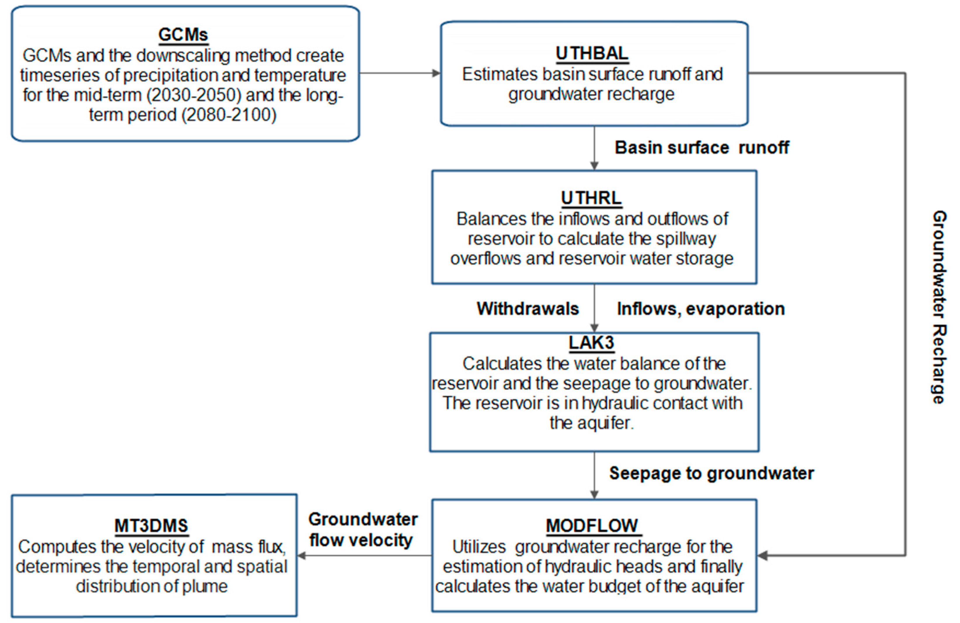
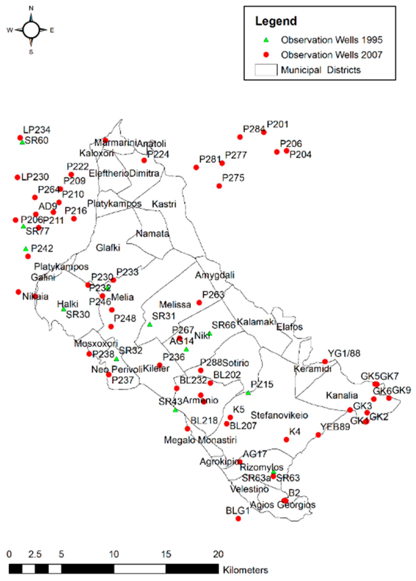
The UTHBAL model was calibrated with the observed sporadic monthly values of Lake Karla’s basin runoff to the Pagasitikos Gulf for the historical period of October 1960 to September 2002, using the multistart Generalized Reduced Gradient algorithm and the split sample test. The Nash–Sutcliffe Model Efficiency was equal to 0.66 for development (using 2/3 of the data selected with random sampling) and validation (using the rest 1/3 of the available streamflow data) periods. The LAK3 model was calibrated against the reservoir’s water level results of the UTHRL model, under the full operation hypothesis. This is due to the absence of historical observed data of the reservoir’s water stages, since the reservoir is still not fully operated in the benefit of the agricultural demands. The Coefficient of Determination (R2) of LAK3 calibration was equal to 0.7805. For the used models UTHRL and LAK3, no validation process was conducted since the reservoir is not in operation yet and no observations are available for validation purposes. The MODFLOW model was calibrated for spatially distributed hydraulic conductivity against 27 observed hydraulic heads for the period of 1997–1987. RMSE was 1.252 and R2 value was 0.989 for the calibration period. The validation period of MODFLOW occurred on May 2002 using 10 wells for the assessment and four statistical criteria (Mean Absolute Error (MAE) = 1.003, RMSE = 1.65, γ = 0.985, and R2 = 0.993). Hence, only the simulation procedure of advection and dispersion of nitrates is presented using the integrated framework to assess natural and man-made effects on groundwater quality. Finally, it is worth mentioning that the dry and wet periods that were used had been characterized on the available historical meteorological data.

3.1. Nitrate Transport and Dispersion Model Calibration

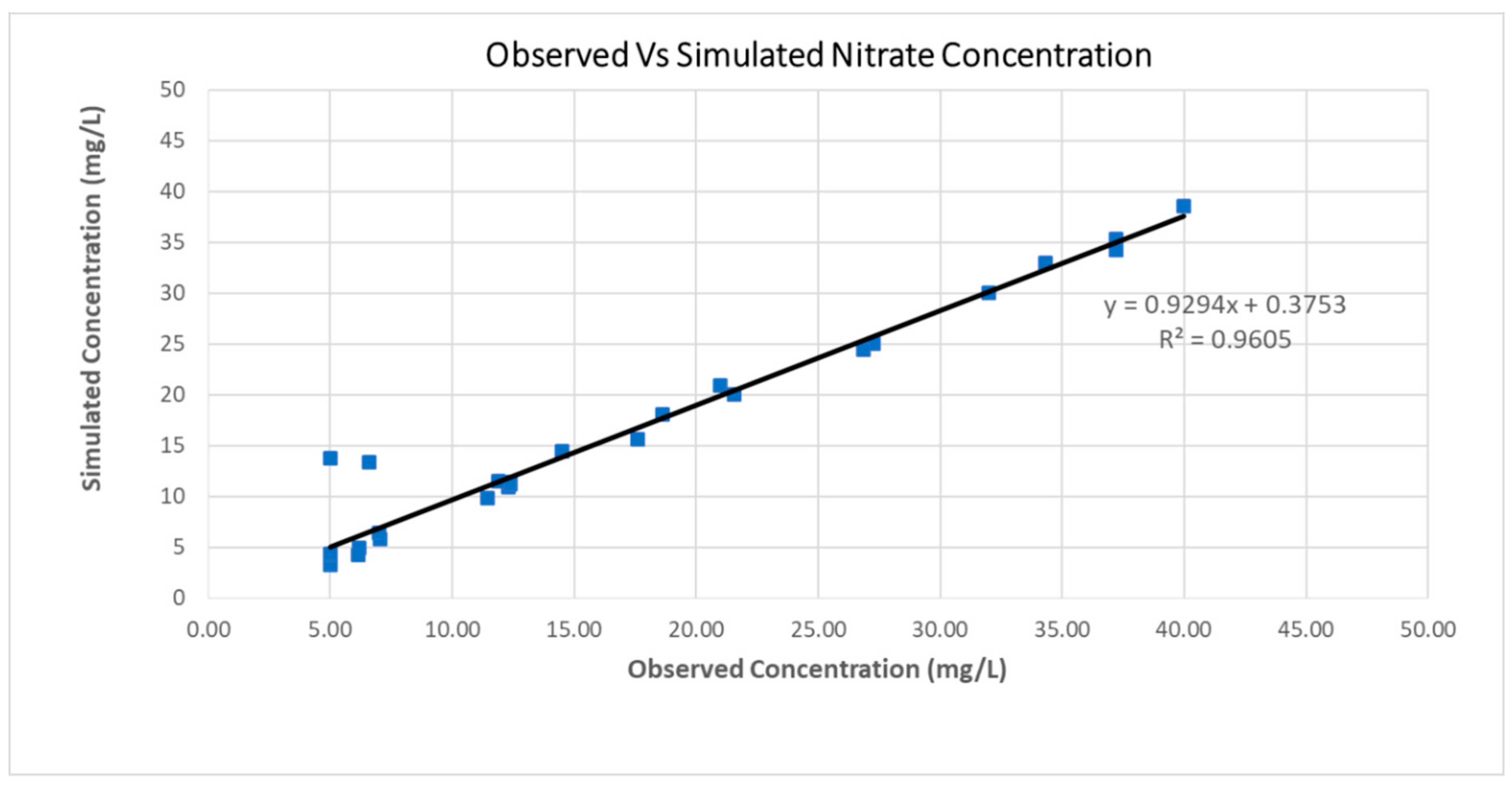
The model calibration procedure is followed in order to assert that the simulated nitrate concentration values are close to the observed ones. The model was calibrated considering the nitrate leaching parameter as the guidance criterion, using the trial and error approach for the observed nitrate concentration data values on 1 September 2007. The visual inspection of Figure 5 (R2 = 0.96) and the performance measure explained by the Nash–Sutcliffe model efficiency coefficient (Ef = 0.95) demonstrated the successful calibration process. The validation process of MT3DMS took place on September 2008 and 22 wells were used. Moreover, the statistical parameter R2 was used for the validation period and it was equal to 0.83. Table 2 shows the starting and final parameter values before-and-after the calibration process of the most significant crops.

3.2. Operation Strategies Results

The operational strategies were performed for the historical period 1995–2007. In these strategies no water demand sub-scenarios were examined. The results regarding to the hydrological modeling on watershed level, were performed by the UTHBAL, UTHRL and LAK3 models and described in the paper of Tzabiras et al. [40]. As expected, between the two scenarios, there was no difference in UTHBAL results as the climatic conditions were the same. Furthermore, there were no UTHRL and LAK3 results for the non-reservoir scenario. However, for the reservoir scenario, UTHRL resulted in a positive volumetric water budget of the aquifer and LAK3 calculated the annual seepage volume at 18 hm3 into the aquifer. These results are fundamental and used as input data of the groundwater nitrate contamination modeling system.

3.2.1. Groundwater Hydrological Modeling

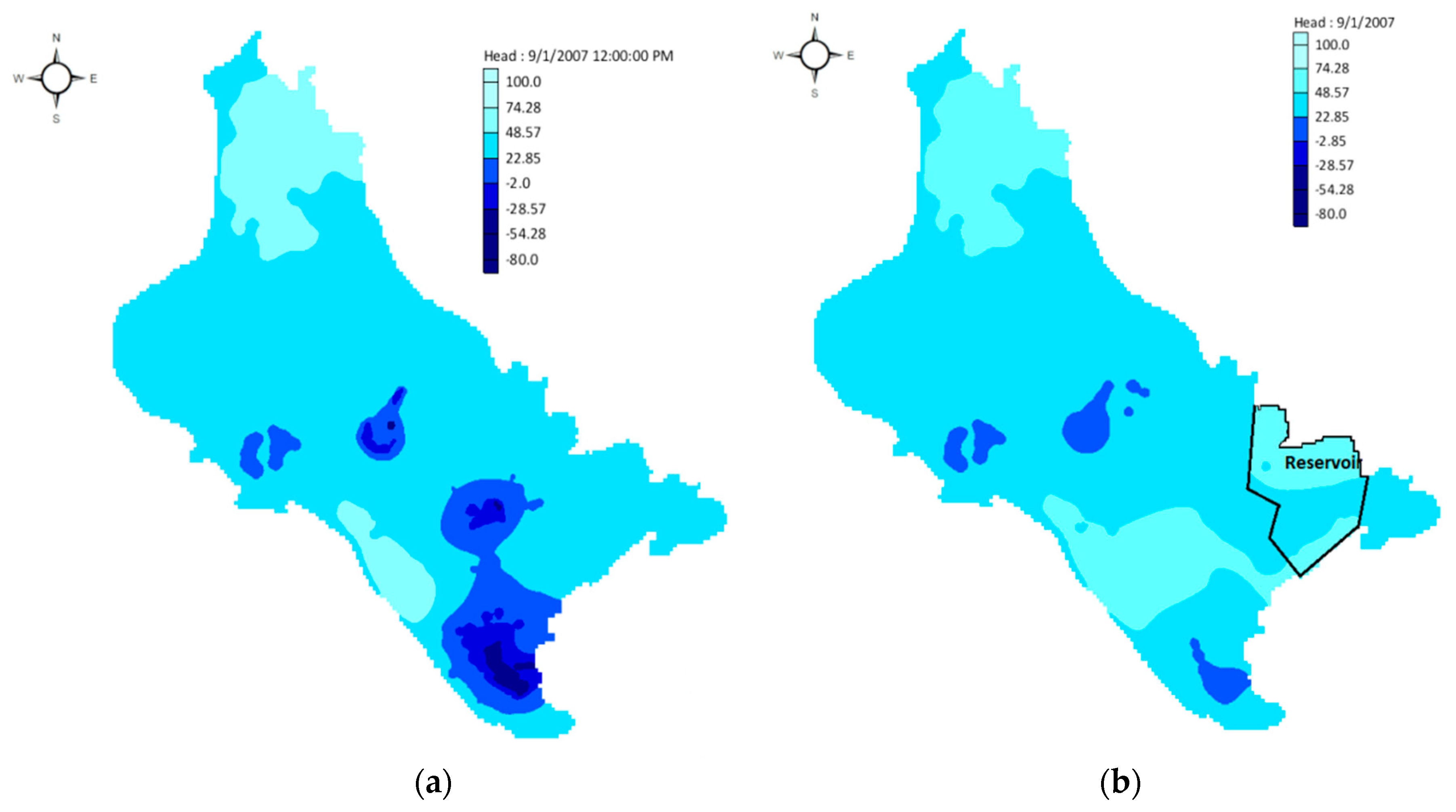
Annually observed water withdrawals of 80 hm3 from the non-renewable resources of the subsurface water system for the no-reservoir scenario described the aquifer’s over-exploitation. As a result, the hydraulic head reached the value of −80 m at the south part of the aquifer area, which is depicted in Figure 6a. On the reservoir scenario implementation, although 62 hm3 per year were exploited from the non-renewable resources, there was a significant rehabilitation of aquifer’s water table at nearby reservoir areas including the southern area of the aquifer (Figure 6b).

3.2.2. Nitrate Transport and Dispersion Modelling

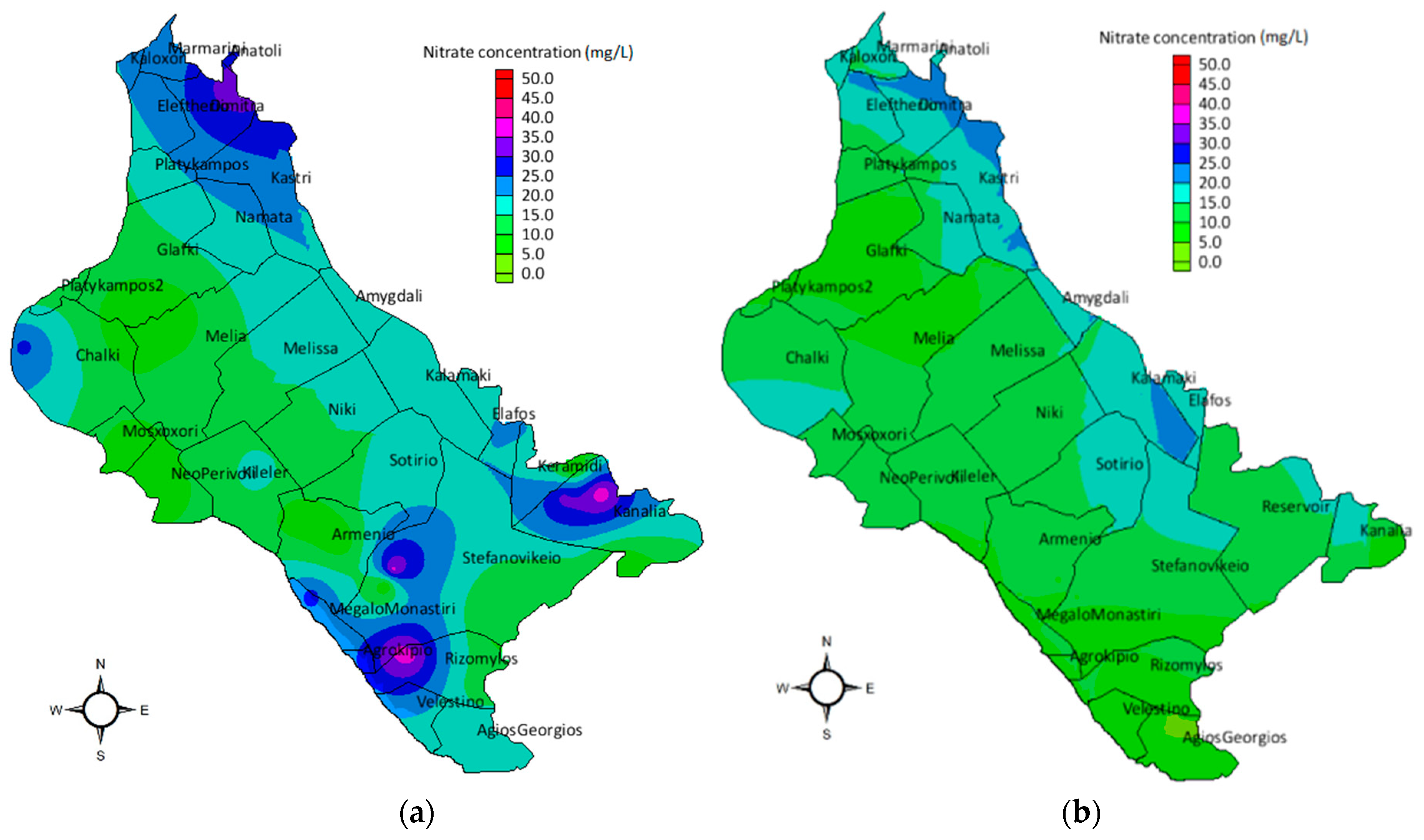
The spatial distribution of nitrate concentration values regarding the no-reservoir scenario, was modelled and presented in Figure 7a. The nitrate values were significantly increased, reaching 33 mg/L in the south-western and south-eastern part of the study area. The large nitrate concentration values were attributed to the excessive application of nitrogenous fertilizers and to the prevailing crop pattern on the study area. According to the reservoir scenario, the results of nitrate concentration values were considerably lower than the no-reservoir scenario. The reservoir operation scenario signaled the increased recharge which is also explained by the direct hydraulic connection between the reservoir and the aquifer. The spatial distribution of its nitrate concentration values is presented in Figure 7b. The maximum nitrate concentration value was equal to 24 mg/L and the lower ones were mostly observed in the south-eastern part of the aquifer, where the reservoir is located. Hence, as nitrates are water-soluble contaminants and the recharge rate is considerably increased, the combination of these two factors resulted in the decrease and dissolution of nitrates in the aquifer. Comparatively evaluating the two management scenarios, the percentages of differences of nitrate concentrations in the surrounding area of the reservoir, ranged between 10% and 15%. Thus, it can be concluded that the contribution of the reservoir operation is of critical importance towards the remediation of the groundwater quality.
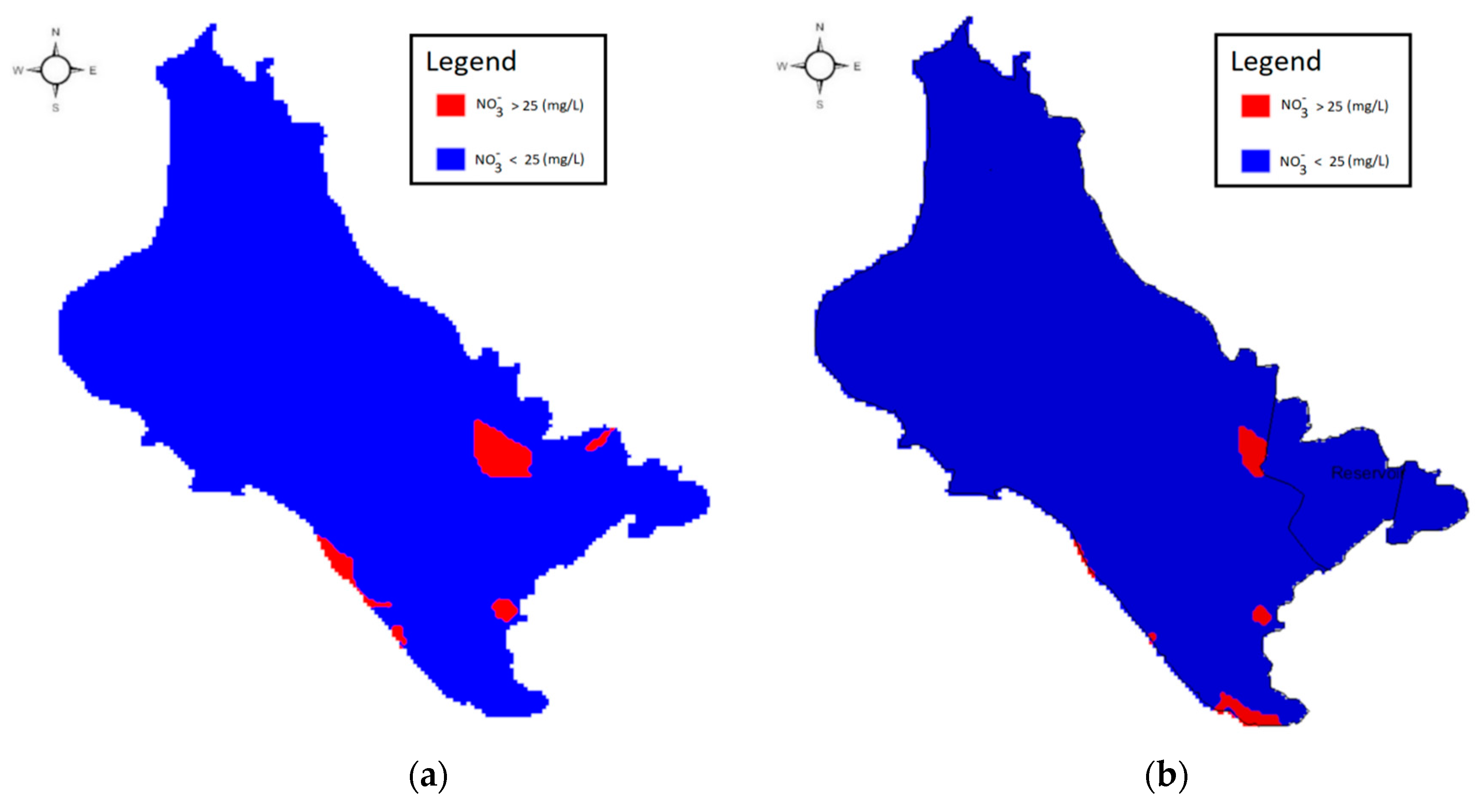
The maximum allowable nitrate concentration limit according to Directive 98/83/EC is the value of 50 mg/L, while the upper limit of 25 mg/L is also defined as the ‘‘guidance value’’, above which the water is characterized as not appropriate for domestic use, since above the defined nitrate upper threshold, severe health issues are caused. The nitrate transport modeling of the no-reservoir scenario showed gradually increasing concentrations of the nitrate compounds in the aquifer, in analogy to the fertilizer application rates on the studied area. The presence of the reservoir, conversely, leads to the increased reservoir’s recharge and the decrease of nitrate concentrations in the groundwater system. Furthermore, the reservoir operation leads to local decrease of nitrate concentrations in the surrounding areas, even below the upper indicative threshold of 25 mg/L, as shown in Figure 8a. Regions with nitrate concentrations above the indicative threshold of 25 mg/L for both the no-reservoir and the reservoir scenario, respectively, are depicted in Figure 8b. As a result, for the inversion of this environmental degradation and the prevention of water pollution, radical measures should be taken for the study area, following the application of good agricultural practices, and the adoption of efficient irrigation methods for the no-reservoir scenario.

3.3. Climate Change Results

3.3.1. Surface Hydrological Modeling

Groundwater recharge is the most essential hydrological component factor that affects nitrate leaching in the aquifer. The annual rainfall decrease observed in all three socioeconomic climatic scenarios has direct impact on the groundwater recharge rates. Annual average recharge rate was estimated to be 41.7 hm3 for the historical period. For the mid-term period of 2030–2050, annual recharge rate is estimated to be 40.7 hm3 for the SRESB1 scenario, 40.5 hm3 for the SRESA1B scenario, and 39.1 hm3 for the most adverse scenario SRESA2. For the long-term period of 2080–2100, it is estimated to be 40.2 hm3 for the SRESB1 scenario, 37.9 hm3 for the SRESA1B scenario, and 37.3 hm3 for the SRESA2 scenario [40].

3.3.2. Groundwater Hydrological Modeling

The overall simulation results highlight the impact of climate change and the effectiveness of the three sub-scenarios of two water resources strategies on the groundwater quantity regime, as shown in Table 3 and Table 4. More specifically, applying of the two water resources management scenarios, the sub-scenarios, and the socioeconomic storylines for the mid and long-term period, the average hydraulic head drawdown was estimated at about 200 m. The largest drawdown (210.73 m) was observed in the mid-term period of the SRESA1 socioeconomic scenario. For the SRESB1 scenario, the drawdown reached the value of 231.40 m for the mid and long-term periods.

3.3.3. Nitrate Solute and Transport Model

The nitrate concentration results which were estimated for the two operational strategies indicated significant differences. Conversely, the resulting differences were minimized during the application of the three socio-economic storylines. The groundwater nitrate contamination results of the two operational scenarios for the historical period and for the three socioeconomic storylines are presented in Table 5 and Table 6.
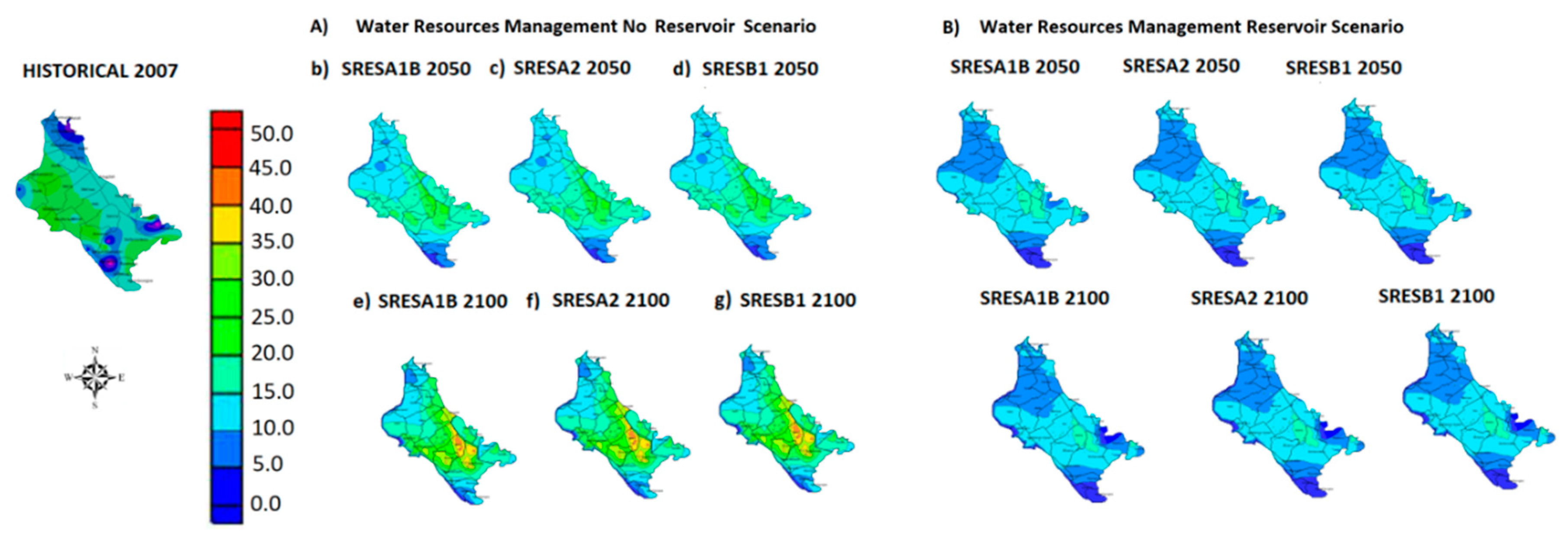
The maximum nitrate concentration value range increased from 31.87 mg/L in the mid-term period, to about 50 mg/L in the long-term period due to climate change without antropogenic activities (no reservoir operation). The highest values of nitrate concentrations was recorded to be 50.48 mg/L in the long-term period of the SRESA2 scenario. Furthermore, the highest values of nitrate concentration were observed at the south-eastern region and portrayed in Figure 9. Additionally, the lowest values of nitrate concentrations were recorded in the mid-term period of the SRESA1B scenario in the north-eastern and south-western part of the study area and are also presented in Figure 9. On the contrary, the nitrate concentration values ranged from 0.20 to 32.64 mg/L, in the historical period. The maximum nitrate concentration value of 32.64 mg/L was recorded in the southeastern area while the minimum value was encountered in the northern part of the study area.
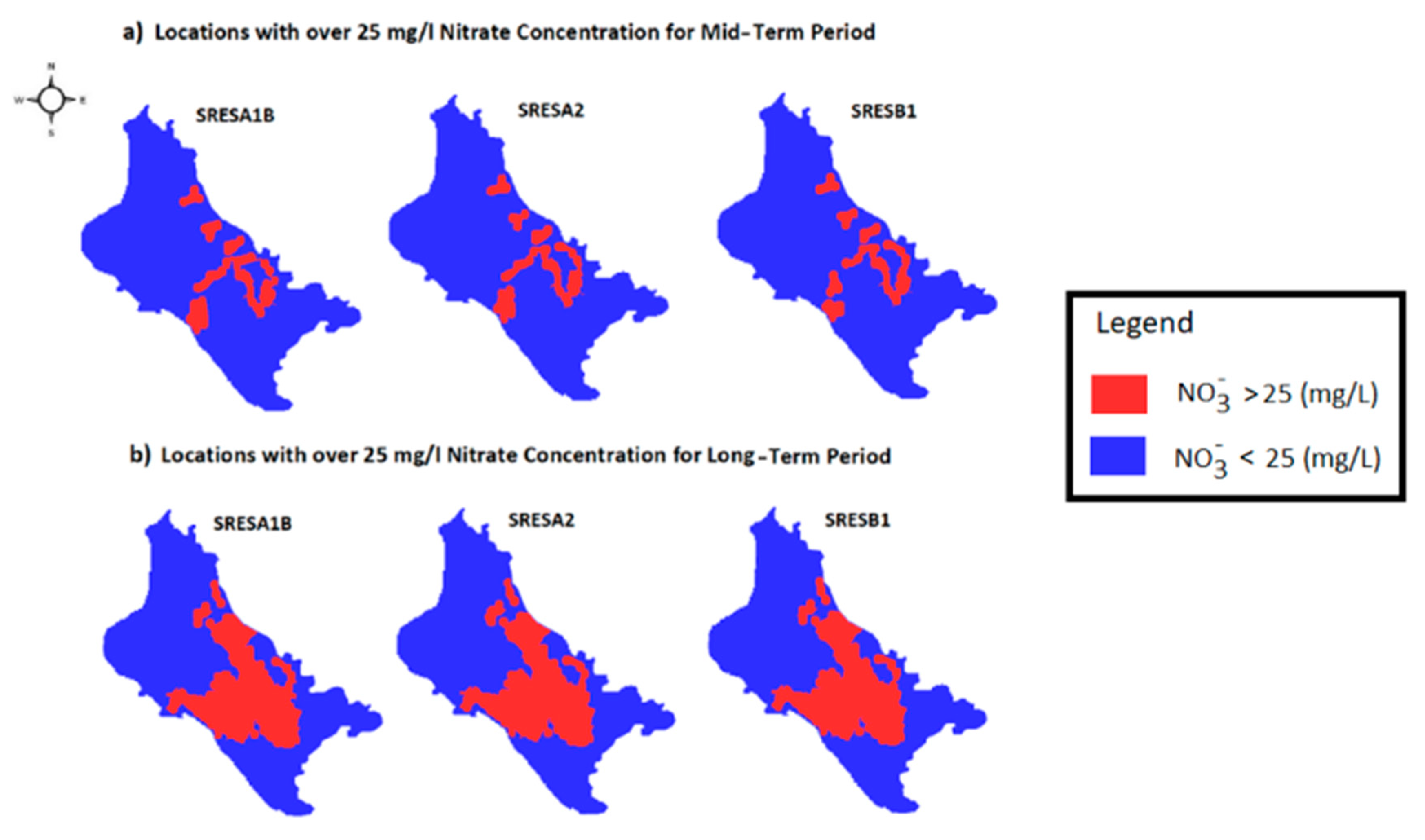
Spatial nitrate concentrations that exceed the indicative threshold value of 25 mg/L regarding the mid-term and long-term period, are depicted in Figure 10a,b, respectively. The comparison of Figure 8 and 
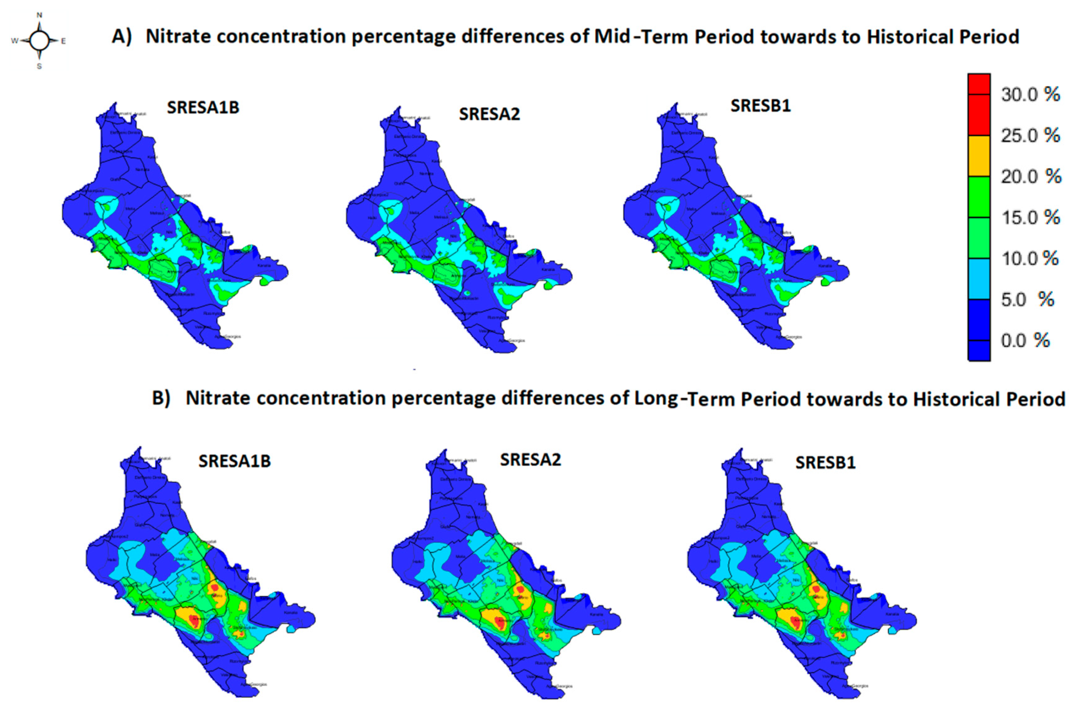
Figure 10 reveal the impact of climate change on nitrate concentrations, since the areas where the value of 25 mg/L is exceeded for the two future periods are significantly larger than the one for the historical period. The percent differences between the three socio-economic plots and the historical period range between 0% and 15% for the mid-term period, and between 0% and 30% for the long-term. Their spatial distribution is illustrated in Figure 11. The differences for the historical period of the reservoir scenario are not depicted, because in neither of the operational nor the climate scenarios was the indicative value of 25 mg/L exceeded. The groundwater quality spatial status for the two water resources operational scenarios in conjunction with the climate change storylines is shown in Figure 9. The above results highlight the necessity of continuous monitoring of groundwater quality in the study area, since many wells are used to supply water for domestic and irrigation uses in the surrounding settlements and in the city of Volos [34].

4. Discussion

One of the most important impacts of climate change and variability on water resources is the reduction of groundwater recharge rate and aquifers’ water table depletion [17,32,33]. This fact affects groundwater quality, leading to the increase of nitrates concentration [17,31,61]. In our research, for the long-term period of SREA2 scenario without reservoir operation, groundwater recharge was reduced to 4.4 hm3 per year and hydraulic head drawdown reached 45 m resulting to about 18 mg/L increase of nitrates concentration. Furthermore, the area of 25 mg/L nitrate concentrations exceedance of aquifer was expanded due to the climate change impact.
On the contrary, the water storage infrastructures operation contributes to the groundwater recharge raise due to their hydraulic connection with the underneath aquifer [62,63]. In the cases where these infrastructures cover the irrigation needs of the nearby cultivations, a significant rehabilitation of aquifer water table was observed [64,65]. The results of this study highlight this benefit. Reservoir operation, for the historical period, increased the groundwater recharge to 18 hm3 per year. Therefore, an elevation of the hydraulic heads at 40 m leading to a reduction of 20 mg/L nitrates concentration was observed in the reservoir vicinity. This concluded to a 41% area reduction of 25 mg/L exceedance.
The land use and the hydrological and hydrogeological data used in this study, refer to the historical period 1995–2007. Newer land use data have been compared with the relevant data of 2001 and the changes were found to be marginal. On the other hand, newer datasets of hydrological and groundwater data are not available. All the component models of the modelling system were calibrated successfully, indicating that the models were able to simulate accurately the hydrological and hydrogeological processes of the watershed and the aquifer of the study area. The calibrated models were also able to capture the future hydrological response because there were no significant changes in the state parameters of the surface and groundwater hydrological processes. Therefore, the use of older datasets was acceptable. They did not introduce additional uncertainties in the results of the paper, and they did not affect the conclusions of the paper.

5. Conclusions

The present study described and evaluated the applicability of an integrated modeling system approach on water management strategies and climate change impacts assessment on the water resources quantity and quality of the Lake Karla aquifer. Nitrates are the most important pollutant factor and nitrate pollution is a known global issue according to worldwide scientific literature, which is caused by the need for increased food-supply production to address the needs of the growing world population. The modeling system included coupled surface, groundwater, and reservoir’s operation hydrological simulation tools that clearly focused on the advection and dispersion of nitrate mass in the groundwater regime.
The groundwater quantity and quality regimes were examined on Municipal District level. Overall, six original water management strategies were compared and evaluated. Two management strategies described the aquifer’s status, one without taking under consideration the operation of the reservoir (no-reservoir scenario) and one taking it under consideration (reservoir scenario). Both cases were sub-linked to three water demand strategies. The climate change impacts were also evaluated for three socio-economic storylines. The applied water resources management strategies’ simulation results under climate change scenarios were milder for the mid-term period, as compared to ones for the long-term period that were more moderate as impact results. Regarding the nitrate contamination of groundwater resources, the management strategies and the current crop pattern applied continued to have significant negative impacts on the groundwater quality regime.
Based on the simulation results, it is concluded that the current agricultural activities were the main reason for the groundwater quality degradation. This phenomenon becomes more intense with climate change impacts. Operational management practices in conjunction with water demands methods compensated the groundwater resources nitrate contamination of climate change impacts. Although the reservoir’s operation in the study area is evidently an efficient groundwater resources management tool, promoting not only the sustainability of the general water regime, but also the regional socio-economic development, this approach of groundwater resources recovery alone, is not a panacea. The adoption and implementation of good agricultural practices in conjunction with the application of appropriate crop pattern, that comply with the objectives of water resources quality remediation constitutes a great necessity.

Author Contributions

P.S. applied and simulated the groundwater flow as well as the reservoir operation simulation. G.T. and P.S. applied and simulated the advection and dispersion of nitrates and created the maps using GIS. L.V. applied and simulated GCMs, the surface hydrological processes and the inflows and outflows of the reservoir. Finally, N.M. and A.L. had the supervision of all the process as well as the supervision of writing the paper.

Funding

This research was funded by Stavros Niarchos Foundation and State Scholarships Foundation.

Acknowledgments

Pantelis Sidiropoulos is a post-doctoral scholar of Stavros Niarchos Foundation and the University of Thessaly. The scientific publication was held within the framework of the invitation “Granting of scholarship for Post-Doctoral Research” of the University of Thessaly, which is being implemented by the University of Thessaly and was funded by the Stavros Niarchos Foundation. Georgios Tziatzios has been co-financed by Greece and the European Union (European Social Fund - ESF) through the Operational Programme Human Resources Development, Education and Lifelong Learning in the context of the project “Scholarships programme for post-graduate studies—2nd Study Cycle” (MIS-5003404), implemented by the State Scholarships Foundation (ΙΚΥ). We are immensely grateful to Konstantina Konovesi and Konstantinos Lois from OPEKEPE for the cultivation and crop data series during the years 2006 and 2007. We would also like to show our gratitude to Georgia Pappa and Ioannis Chrysiados from the Ministry of Rural Development and Food, Directorate General of Administrative Services and eGovernment, Data Center Network Center, Records, Databases and Data Statistics in Bibliography for the cultivation and crop data series from 1995 to 2005.

Conflicts of Interest

The authors declare no conflict of interest.

References

  1. Jajarmizadeh, M.; Harun, S.; Salarpour, M. A review on theoretical consideration and types of models in hydrology. IJEST 2012, 5, 249–261. [Google Scholar] [CrossRef]
  2. Biswas, A.K. Integrated water resources management: Is it working? Int. J. Water Resour. 2008, 24, 5–22. [Google Scholar] [CrossRef]
  3. Li, L.; Zongxue, X.; Depeng, Z.; Jie, Z. A grid-based integrated surface–groundwater model (GISMOD). J. Water Clim. Chang. 2015, 7, 296–320. [Google Scholar] [CrossRef]
  4. Jaworska-Szulc, B. Role of the Lakes in groundwater recharge and discharge in the Young Glacial area, Northern Poland. Ground Water 2016, 54, 603–611. [Google Scholar] [CrossRef] [PubMed]
  5. Candela, L.; Von Igel, W.; Javier Elorza, J.F.; Aronica, G. Impact assessment of combined climate and management scenarios on groundwater resources and associated wetland (Majorca, Spain). J. Hydrol. 2009, 376, 510–527. [Google Scholar] [CrossRef]
  6. Simon, B.R.; Bernard, S.; Meurville, C.; Rebour, V. Flow-through stream modeling with MODFLOW and MT3D: Certainties and limitations. Ground Water 2015, 53, 967–971. [Google Scholar] [CrossRef]
  7. Spalding, R.F.; Exner, M.E. Occurrence of nitrate in groundwater—A review. J. Environ. Qual. 1993, 22, 392–402. [Google Scholar] [CrossRef]
  8. Voudouris, K.; Panagopoulos, A.; Koumantakis, I. Nitrate pollution in the coastal aquifer system of the Korinthos (Greece). Glob. Nest J. 2004, 6, 11–18. [Google Scholar]
  9. Molénat, J.; Gascuel-Odoux, C. Modelling flow and nitrate transport in groundwater for the prediction of water travel times and of consequences of land use evolution on water quality. Hydrol. Process. 2002, 16, 479–492. [Google Scholar] [CrossRef]
  10. Papaioannou, A.; Plageras, P.; Dovriki, E.; Minas, A.; Krikelis, V.; Nastos, P.T.; Kakavas, K.; Paliatsos, A.G. Groundwater quality and location of productive activities in the region of Thessaly (Greece). Desalination 2007, 213, 209–217. [Google Scholar] [CrossRef]
  11. Ghiglieri, G.; Barbieri, G.; Vernier, A.; Carletti, A.; Demurtas, N.; Pinna, R.; Pittalis, D. Potential risks of nitrate pollution in aquifers from agricultural practices in the Nurra region, northwestern Sardinia, Italy. J. Hydrol. 2009, 379, 339–350. [Google Scholar] [CrossRef]
  12. Peña-Haro, S.; Velazquez, P.M.; Sahuquillo, A. A hydro-economic modelling framework for optimal management of groundwater nitrate pollution from agriculture. J. Hydrol. 2010, 373, 193–203. [Google Scholar] [CrossRef]
  13. Takounjou, F.A.; Kuitcha, D.; Fantong, W.Y.; Ewodo, M.G.; Khan, H.H.; Isssa, O.T. Assessing groundwater nitrate pollution in Yaoundé, Cameroon: Modelling approach. World Appl. Sci. J. 2013, 23, 333–344. [Google Scholar] [CrossRef]
  14. Sharma, M.K.; Jain, C.K.; Rao, G.T.; Gurunadha Rao, V.V.S. Modelling of lindane transport in groundwater of metropolitan city Vadodara, Gujarat, India. Environ. Monit. Assess. 2015, 187. [Google Scholar] [CrossRef] [PubMed]
  15. Almasri, M.N.; Kaluarachchi, J.J. Modeling nitrate contamination of groundwater in agricultural watersheds. J. Hydrol. 2007, 343, 211–229. [Google Scholar] [CrossRef]
  16. Shamrukh, M.; Corapcioglu, M.Y.; Hassona, F.A.A. Modeling the effect of chemical fertilizers on groundwater quality in the Nile Valley aquifer. Ground Water 2001, 39, 59–67. [Google Scholar] [CrossRef]
  17. Paradis, D.; Vigneault, H.; Lefebvre, R.; Savard, M.M.; Ballard, J.M.; Qian, B.D. Groundwater nitrate concentration evolution under climate change and agricultural adaptation scenarios: Prince Edward Island, Canada. Earth Syst. Dyn. 2016, 7, 183–202. [Google Scholar] [CrossRef] [Green Version]
  18. Ghoraba, S.M.; Zyedan, B.A.; Rashwan, I.M.H. Solute transport modeling of the groundwater for quaternary aquifer quality management in Middle Delta, Egypt. Alexandria Eng. J. 2013, 52, 197–207. [Google Scholar] [CrossRef] [Green Version]
  19. Psaropoulou, E.T.; Karatzas, G. Pollution of nitrates contaminant transport i heterogeneous porous media: A case study of the coastal aquifer of Corinth, Greece. Glob. Nest J. 2014, 16, 9–23. [Google Scholar] [CrossRef]
  20. Serio, F.; Miglietta, P.P.; Lamastra, L.; Ficocelli, S.; Intini, F.; De Leo, F.; De Donno, A. Ground water nitrate contamination and agricultural land use: A grey water footprint perspective in Southern Apulia Region (Italy). Sci. Total Environ. 2018, 645, 1425–1431. [Google Scholar] [CrossRef]
  21. Gemitzi, A.; Petalas, C.; Pisinaras, V.; Tsihrintzis, V.A. Spatial prediction of nitrate pollution in groundwaters using neural networks and GIS: An application to South Rhodope aquifer (Thrace, Greece). Hydrol. Process. 2009, 23, 372–383. [Google Scholar] [CrossRef]
  22. Lockhart, K.M.; King, A.M.; Harter, T. Identifying sources of groundwater nitrate contamination in a large alluvial groundwater basin with highly diversified intensive agricultural production. J. Contam. Hydrol. 2013, 151, 140–154. [Google Scholar] [CrossRef] [PubMed]
  23. Almasri, M.N.; Kaluarachchi, J.J. Multi-criteria decision analysis for the optimal management of nitrate contamination of aquifers. J. Environ. Manag. 2005, 74, 365–381. [Google Scholar] [CrossRef] [PubMed] [Green Version]
  24. Powlson, D.S.; Addiscott, T.M. Nitrogen in Soils, Nitrates, Encyclopedia of Soils in the Environment, 1st ed.; Hinnel, D.A., Rosenzweig, C.B., Polson, S.D.C., Scow, M.K., Singer, J.M., Sparks, L.D., Eds.; Academic Press, Elsevier: New York, NY, USA, 2005; pp. 21–56. ISBN1 10:0123485304. ISBN2 13:978-0123485304. [Google Scholar]
  25. Liu, C.W.; Lin, C.N.; Jang, C.S.; Ling, M.P.; Tsai, J.W. Assessing nitrate contamination and its potential health risk to Kinmen residents. Environ. Geochem. Health 2011, 33, 503–514. [Google Scholar] [CrossRef] [PubMed]
  26. Olesen, E.J.; Bindi, M. Consequences of climate change for European agricultural productivity, land use and policy. Eur. J. Agron. 2002, 16, 239–262. [Google Scholar] [CrossRef]
  27. Roelsma, J.; Hendriks, R.F.A. Comparative study of nitrate leaching models on a regional scale. Sci. Total Environ. 2014, 499, 481–496. [Google Scholar] [CrossRef]
  28. Maran, N.H.; Crispim, B.D.; Iahnn, S.R.; Araújo, R.P.; Grisolia, A.B.; Oliveira, K.M. Depth and well type related to groundwater microbiological contamination. Int. J. Environ. Res. Public Health 2016, 13, 1036. [Google Scholar] [CrossRef]
  29. Shrestha, S.; Bach, V.T.; Pandey, P.V. Climate change impacts on groundwater resources in Mekong Delta under representative concentration pathways (RCPs) scenarios. Environ. Sci. Policy 2016, 61, 1–13. [Google Scholar] [CrossRef]
  30. Pulido-Velazquez, M.; Peña-Haro, S.; García-Prats, A.; Mocholi-Almudever, A.F.; Henriquez-Dole, L.; Macian-Sorribes, H.; Lopez-Nicolas, A. Integrated assessment of the impact of climate and land use changes on groundwater quantity and quality in the Mancha Oriental system (Spain). Hydrol. Earth Syst. Sci. 2015, 19, 1677–1693. [Google Scholar] [CrossRef] [Green Version]
  31. Pascual, D.; Pla, E.; Lopez-Bustins, J.A.; Retana, J.; Terradas, J. Impacts of climate change on water resources in the Mediterranean Basin: A case study in Catalonia, Spain. Hydrol. Sci. J. 2015, 60, 2132–2147. [Google Scholar] [CrossRef]
  32. Taylor, R.G.; Scanlon, B.; Döll, P.; Rodell, M.; Van, B.R.; Wada, Y.; Longuevergne, L.L.M.; Famiglietti, J.S.; Edmunds, M.; Konikow, L.; et al. Ground water and climate change. Nat. Clim. Chang. 2012, 3, 322–329. [Google Scholar] [CrossRef] [Green Version]
  33. Green, T.R.; Taniguchi, M.; Kooi, H.; Gurdak, J.J.; Allen, D.M.; Hiscock, K.M.; Treidel, H.; Aureli, A. Beneath the surface: Impacts of climate change on groundwater. J. Hydrol. 2011, 405, 532–560. [Google Scholar] [CrossRef]
  34. Sidiropoulos, P.; Tziatzios, G.; Vasiliades, L.; Papaioannou, G.; Mylopoulos, N.; Loukas, A. Modelling flow and nitrate transport in an over-exploited aquifer of rural basin using an integrated system: The case of Lake Karla watershed. Proceedings 2018, 2, 667. [Google Scholar] [CrossRef]
  35. Loukas, A.; Mylopoulos, N.; Kokkinos, K.; Sidiropoulos, P.; Vasiliades, L.; Liakopoulos, A. The effect of spatial discretization in integrated modeling of surface and groundwater hydrology through OpenMI. In Proceedings of the International Interdisciplinary Conference on Predictions for Hydrology, Ecology and Water Resources Management—Using Data and Models to Benefit Society, Prague, Czech Republic, 15–18 September 2008. [Google Scholar]
  36. Sidiropoulos, P.; Mylopoulos, N.; Loukas, A. Stochastic simulation and management of an over-exploited aquifer using an integrated modeling system. Water Resour. Manag. 2015, 29, 929–943. [Google Scholar] [CrossRef]
  37. Intergovernmental Panel on Climate Change IPCC. Climate Change 2007—The Physical science basis. In Contribution of Working Group I to the Fourth Assessment Report of the Intergovernmental Panel on Climate Change (IPCC); Solomon, S., Qin, D., Manning, M., Chen, Z., Marquis, M., Averyt, K.B., Tignor, M., Miller, H.L., Eds.; Cambridge University Press: Cambridge, UK, 2007. [Google Scholar]
  38. Kløve, B.; Ala-Aho, P.; Bertrand, G.; Gurdak, J.J.; Kupfersberger, H.; Kvoerner, J.; Muotka, T.; Mykrä, H.; Preda, E.; Rossi, P.; et al. Climate change impacts on groundwater and dependent ecosystems. J. Hydrol. 2014, 518, 250–266. [Google Scholar] [CrossRef]
  39. Tzabiras, J.; Vasiliades, L.; Loukas, A.; Mylopoulos, N. Climate change impacts on hydrometeorological variables using a bias correction method. The Lake Karla watershed case. MESA J. 2015, 6, 683–700. [Google Scholar]
  40. Tzabiras, J.; Vasiliades, L.; Sidiropoulos, P.; Loukas, A.; Mylopoulos, N. Evaluation of water resources management strategies to overturn climate change impacts on Lake Karla watershed. Water Resour. Manag. 2016, 30, 5819–5844. [Google Scholar] [CrossRef]
  41. Moss, R.H.; Edmonds, J.A.; Hibbard, K.A.; Manning, M.R.; Rose, S.K.; Van Vuuren, D.P.; Carter, T.R.; Emori, S.; Kainuma, M.; Kram, T.; et al. The next generation of scenarios for climate change research and assessment. Nature 2010, 463, 747–756. [Google Scholar] [CrossRef]
  42. Alotaibi, K.; Ghumman, A.; Haider, H.; Ghazaw, Y.; Shafiquzzaman, M. Future predictions of rainfall and temperature using GCM and ANN for arid regions: A case study for the Qassim Region, Saudi Arabia. Water 2018, 10, 1260. [Google Scholar] [CrossRef]
  43. Loukas, A.; Mylopoulos, N.; Vasiliades, L. A modeling system for the evaluation of water resources management strategies in Thessaly, Greece. Water Resour. Manag. 2007, 21, 1673–1702. [Google Scholar] [CrossRef]
  44. Merritt, M.L.; Konikow, L.F. Documentation of a Computer Program to Simulate Lake-Aquifer Interaction Using the MODFLOW Ground-Water Flow Model and the MOC3D Solute-Transport Model; Water-Resources Investigations Report 00–4167; U.S. Geological Survey: Reston, VA, USA, 2000.
  45. Harbaugh, A.W.; McDonald, M.G. User’s Documentation for MODFLOW-2000, an Update to the U.S. Geological Survey Modular Finite-Difference Ground-Water Flow Model; United States Government Printing Office: Washington, DC, USA, 2000.
  46. Zheng, C.; Wang, P.P. MT3DMS: A Modular Three-Dimensional Multi-Species Transport Model for Simulation of Advection, Dispersion and Chemical Reactions of Contaminants in Groundwater Systems, Documentation and User’s Guide; Army Corps of Engineers: Washington, DC, USA, 1999. [Google Scholar]
  47. Costantinidis, D. Hydrodynamique d’un système aquifère hétérogène, Hydrogéologie de la Thessalie Orientale. Ph.D. Thesis, University of Grenoble, Grenoble, France, 1978. [Google Scholar]
  48. Craig, J.R.; Rabideau, A.J. Finite element transport modeling using analytic element flow solutions. Water Resour. Res. 2006, 42, 1–16. [Google Scholar] [CrossRef]
  49. Konikow, F.L. The secret to successful solute-transport modeling. Ground Water 2011, 49, 144–159. [Google Scholar] [CrossRef] [PubMed]
  50. Schulze-Makuch, D. Longitudinal dispersivity data and implications for scaling behavior. Ground Water 2005, 43, 443–456. [Google Scholar] [CrossRef] [PubMed]
  51. Gelhar, L.; Welty, C.; Rehfeldt, K.A. Critical review of data on field-scale dispersion in aquifers. Water Resour. Res. 1992, 28, 1955–1974. [Google Scholar] [CrossRef]
  52. Institute of Geological and Mineral Exploration. Recording and Evaluation of the Hydrogeological Characteristics of the Groundwater Systems of the Country; Basement of the Aquatic Potential of Thessaly; Institute of Geological and Mineral Exploration: Thessaloniki, Greece, 2010. [Google Scholar]
  53. Libutti, A.; Monteleone, M. Soil vs. groundwater: The quality dilemma. Managing nitrogen leaching and salinity control under irrigated agriculture in Mediterranean conditions. Agric. Water Manag. 2017, 186, 40–50. [Google Scholar] [CrossRef]
  54. Kourakos, G.; Harter, T. Parallel simulation of groundwater non-point source pollution using algebraic multigrid preconditioners. Computat. Geosci. 2014, 18, 851–867. [Google Scholar] [CrossRef]
  55. Almasri, M.N.; Kaluarachchi, J.J. Implications of on-ground nitrogen loading and soil transformations on ground water quality management. JAWRA 2004, 40, 165–186. [Google Scholar] [CrossRef]
  56. Doble, M.; Kumar, A. Groundwater Decontamination and Treatment. In Biotreatment of Industrial Effluents, 1st ed.; Elsevier: Amsterdam, The Netherlands; Butterworth-Heinemann: New York, NY, USA, 2005; pp. 285–294. ISBN 9780750678384. [Google Scholar]
  57. Burkart, M.R.; Stoner, D.J. Nitrate in aquifers beneath agricultural systems. Water Sci. Technol. 2007, 56, 59–69. [Google Scholar] [CrossRef]
  58. Wichmann, W. World Fertilizer Use Manual; International Fertilizer Association: Paris, France, 1992. [Google Scholar]
  59. Ministry of Rural Development and Food. Data on the Integrated Management System of Cultivated Areas; Ministry of Rural Development and Food: Athens, Greece, 1995–2007.
  60. Pisinaras, V.; Petalas, C.; Tsihrintzis, V.A.; Zagana, A. A groundwater flow model for water resources management in the Ismarida plain, North Greece. Environ. Model. Assess. 2007, 12, 75–89. [Google Scholar] [CrossRef]
  61. Antonakos, A.; Lambrakis, N. Hydrodynamic characteristics and nitrate propagation in Sparta aquifer. Water Resour. Res. 2000, 34, 3977–3986. [Google Scholar] [CrossRef]
  62. Zajac, Z.; Revilla-Romero, B.; Salamon, P.; Burek, P.; Hirpa Feyera, A. The impact of lake and reservoir parameterization on global streamflow simulation. J. Hydrol. 2016, 548, 552–568. [Google Scholar] [CrossRef] [PubMed]
  63. Yihdego, Y.; Webb, J.A.; Vaheddoost, B. Highlighting the role of groundwater in lake—Aquifer interaction to reduce vulnerability and enhance resilience to climate change. Hydrology 2017, 4, 10. [Google Scholar] [CrossRef]
  64. Seeboonruang, U. Impacts of reservoir on groundwater level and quality in a Saline Area, Nakhon Panom Province, Thailand. APCBEE Procedia 2012, 4, 16–21. [Google Scholar] [CrossRef]
  65. Guo, W. Transient groundwater flow between reservoirs and water-table aquifers. J. Hydrol. 1997, 195, 370–384. [Google Scholar] [CrossRef]
Figure 1. The study idea and its hydrogeological formations.
Water 11 01201 g001
Figure 2. Land Uses and Crop Classification in 2001.
Water 11 01201 g002
Figure 3. Flow chart of Modelling System Framework.
Water 11 01201 g003
Figure 4. Location of observation wells for the simulation period.
Water 11 01201 g004
Figure 5. Scatter diagram of observed versus simulated nitrate concentration values for the study area on 1 September 2007. The equation of the linear regression and the R2 value are also presented.
Water 11 01201 g005
Figure 6. Hydraulic head results of the operational scenarios modeling: (a) No-reservoir scenario hydraulic heads; (b) reservoir scenario hydraulic heads.
Water 11 01201 g006
Figure 7. Nitrate concentrations on the operational scenarios modeling: (a) No-reservoir scenario nitrate concentrations; (b) reservoir scenario nitrate concentrations.
Water 11 01201 g007
Figure 8. Spatial location of over 25 mg/L nitrate concentrations: (a) No-reservoir scenario and (b) reservoir scenario.
Water 11 01201 g008
Figure 9. Maps of Nitrate concentration for the two water resources management and socio-economic scenarios: (A) SRES scenario of no-reservoir operational strategy; and (B) SRES scenario of reservoir operational strategy.
Water 11 01201 g009
Figure 10. Spatial distribution of 25 mg/L excess for all three socio-economic scenarios for the historical period of no-reservoir scenario: (a) For Mid-Term Period of 2030–2050 and (b) for Long-Term Period of 2080–2100.
Water 11 01201 g010
Figure 11. Nitrate concentration percentage differences for all three social-economic scenarios towards to the historical period of no-reservoir status: (A) Mid-Term Period and (B) Long-Term Period.
Water 11 01201 g011
Table 1. Land Uses and Crop Classification percentage area.
CropsArea km2Percentage (%)
Cotton114.4722.89
Wheat153.1930.64
Energy Crops0.280.06
Legumes14.382.88
Maize12.292.46
Cereals32.236.45
Sugar Beets8.671.73
Pastures37.247.45
Wetland1.910.38
Water Bodies42.288.46
Urban Areas42.818.56
Other Land Uses40.258.05
Total Area500.00100.00
Table 2. Parameters and changes before-and-after calibration of the main crops.
CropsNitrate Loading
Before Calibration (kg/ha/year)After Calibration (kg/ha/year)
Cereal Crops100140
Cotton150240
Energy Crops220310
Legumes030
Maize250330
Sugar Beets115195
Wheat140240
Table 3. Simulation results from MODFLOW for water demand sub-scenarios of no reservoir operation strategy.
MODFLOW Simulation Results
Historical PeriodMid-Term PeriodLong-Term Period
A1BA2B1A1BA2 B1
Hydraulic Head (m)CS sub-scenarioMin −80.60−216.49−146.96−201.37−198.11−218.31−228.32
Max105.5749.8169.8558.6858.6860.0449.82
Mean 44.52−31.6645.817.046.95−16.38−30.97
Median45.81−29.0548.327.797.74−13.30−28.19
Standard deviation0.971.622.182.312.332.851.65
RCL sub-scenarioMin −80.60−210.59−210.73−200.69−224.14−204.94−225.28
Max105.5758.7558.6858.6849.8149.7849.81
Mean 44.528.377.387.58−27.83−29.40−27.48
Median45.819.107.918.05−23.69−25.55−23.32
Standard deviation0.971.952.021.991.641.671.60
AIM sub-scenarioMin −80.60−208.44−201.37−202.03−224.56−231.40−221.41
Max105.5758.6860.3156.0849.8162.2949.81
Mean 44.527.1919.25−1.30−30.38−12.01−33.06
Median45.817.8118.46−1.93−27.06−7.98−30.08
Standard deviation0.972.212.532.741.701.441.35
Table 4. Simulation results from MODFLOW for water demand sub-scenarios of reservoir operation strategy.
MODFLOW Simulation Results
Historical PeriodMid-Term PeriodLong-Term Period
A1BA2B1A1BA2 B1
Hydraulic Head (m)CS sub-scenarioMin −79.00−201.11−202.25−205.72−223.95−222.59−197.11
Max105.4458.6859.0059.0269.7371.6271.81
Mean 46.5212.276.987.43−8.95−12.41−10.50
Median47.2211.827.518.00−1.93−3.73−1.97
Standard deviation1.012.203.032.941.941.961.72
RCL sub-scenarioMin −79.00−202.22−207.48−201.73−224.73−224.21−229.15
Max105.4458.9959.0059.0271.7171.6271.81
Mean 46.528.338.058.54−8.18−9.25−7.47
Median47.227.947.698.09−3.41−4.33−2.86
Standard deviation1.012.582.642.551.551.611.54
AIM sub-scenarioMin −79.00−203.02−199.75−202.22−221.32−194.98−222.90
Max105.4458.9959.0059.0271.7171.6271.81
Mean 46.527.687.407.87−9.94−11.13−9.19
Median47.227.987.698.21−3.07−4.05−2.66
Standard deviation1.012.822.872.781.641.751.59
Table 5. Simulation results from MT3DMS for water demand sub-scenarios of no reservoir operation strategy.
MT3DMS Simulation Results
Historical PeriodMid-Term PeriodLong-Term Period
A1BA2B1A1BA2 B1
Nitrate Concentration (mg/L)CS sub-scenarioMin 0.200.930.930.920.900.930.95
Max32.6431.8732.4731.7047.7250.4847.18
Mean 14.1313.8613.9613.8418.5418.6618.45
Median13.2913.7613.8413.7517.5317.3517.45
Standard deviation0.870.180.170.170.450.500.44
RCL sub-scenarioMin 0.200.930.930.921.061.051.07
Max32.6430.7331.1331.1749.2648.9351.33
Mean 14.1313.8013.6913.8618.3918.2318.12
Median13.2913.7513.6613.7617.4517.0316.89
Standard deviation0.870.190.210.140.470.500.45
AIM sub-scenarioMin 0.200.930.930.920.980.980.99
Max32.6431.2831.7131.0148.0549.7847.24
Mean 14.1313.8713.6113.8418.5417.9718.44
Median13.2913.7713.2913.7517.5116.9117.43
Standard deviation0.870.180.190.170.460.480.45
Table 6. Simulation results from MT3DMS for water demand sub-scenarios of reservoir operation strategy.
MT3DMS Simulation Results
Historical PeriodMid-Term PeriodLong-Term Period
A1BA2B1A1BA2 B1
Nitrate Concentration (mg/L)CS sub-scenarioMin 0.060.260.260.260.180.170.19
Max24.0420.5820.6920.3720.8420.5620.77
Mean 11.4011.0611.0618.8510.3310.3419.20
Median11.3311.2311.2311.0610.4310.4410.33
Standard deviation0.230.060.050.100.030.030.09
RCL sub-scenarioMin 0.060.260.260.260.220.210.23
Max24.0418.9518.4918.4719.5218.0819.24
Mean 11.4011.0611.2111.2110.5010.5010.49
Median11.3311.2311.1711.1710.4410.4510.43
Standard deviation0.230.063.273.273.243.253.23
AIM sub-scenarioMin 0.060.260.260.230.200.180.15
Max24.0419.6518.5918.7919.0618.5919.98
Mean 11.4011.0611.1011.2110.4910.3610.48
Median11.3311.2310.9811.1710.4310.2310.42
Standard deviation0.230.063.233.273.253.203.27

