Experimental and Numerical Investigation of Mixing Phenomena in Double-Tee Junctions


1
Department of Fluid Mechanics and Computational Engineering, Faculty of Engineering, University of Rijeka, 51000 Rijeka, Croatia
2
Center for Advanced Computing and Modeling, University of Rijeka, 51000 Rijeka, Croatia
*
Author to whom correspondence should be addressed.
Water 2019, 11(6), 1198; https://doi.org/10.3390/w11061198
Submission received: 3 May 2019
/
Revised: 3 June 2019
/
Accepted: 6 June 2019
/
Published: 8 June 2019
(This article belongs to the Section Hydraulics and Hydrodynamics)
Abstract
:This work investigates mixing phenomena in a pressurized pipe system with two sequential Tee junctions and experiments are conducted for a range of different inlet flow ratios, varying distances between Tee junctions and two pipe branching configurations. Additionally, obtained experimental results are compared with results from previous studies by different authors and are used to validate the numerical model using the open source computational fluid dynamics toolbox OpenFOAM. Two different numerical approaches are used—Passive scalar model and Multiphase model. It is found that both numerical models produce similar results and that they are both greatly dependent on the turbulent Schmidt number. After the calibration procedure, both models provided good results for all investigated flow ratios, double-Tee junction distances, and pipe branching configurations, therefore both numerical models can be applied for a wide range of pipe networks configurations, but passive scalar model is the viable choice due to its much higher computational efficiency. Obtained results also describe the relationship between the double-Tee distances and complete mixing occurrence.
1. Introduction
Water distribution networks are complex systems that are of great concern due to the possibility of accidental or deliberate water contamination that can affect a great number of network users. To predict and prevent such scenarios, a number of water-quality models were developed that help in modeling of such complex systems. Most widely used simulation software is EPANET developed by the Environmental Protection Agency [1] which provides quick results of hydraulic and water-quality analysis of complex networks. EPANET can be used in investigation of algorithms and methods for optimal sensor placement [2,3], contaminant source detection [4,5,6] or contaminant characterization [7].
Mass transport at junctions is a complex phenomenon due to secondary currents or flow instabilities that can greatly enhance turbulence and thus mixing. Due to this, a proper mixing model must be known to correctly predict contamination spreading in a pipe network. EPANET assumes complete mixing at every junction, which makes the concentration in the fluid at the outlet pipes the same and its value is defined by the inlet pipe flow-weighted concentrations. While complete mixing model is formulated in accordance with the law of conservation of mass, it can be considered correct only if there is a single outlet at a junction as it does not accurately describe the physical process of mixing. The greatest deviation from complete mixing occurs when the Reynolds numbers are the same for all the inlet and outlet pipes [8]. A water-quality model in EPANET was improved with experimental and three-dimensional computational fluid dynamics (CFD) approach for cross junctions with different inlet and outlet flow scenarios [9]. In turbulent mixing at a cross junction, there is a considerable difference from complete mixing [10]. A bulk advective mixing model (BAM) which describes bulk mixing was developed, instabilities and diffusion of fluid interfaces are ignored and bulk mixing is defined as a lower limit of mixing while complete mixing model represented the upper boundary of mixing behavior [11]. Bulk mixing model greatly depends on the flow momentum in each inlet pipe as it is calculated and used to determine how the inlet concentrations will split into the outlet pipes i.e., the pipe flow with higher momentum will be dominant in spreading the concentration in the outlet pipe with the same direction, while the pipe with the lower momentum flow will only spread to its neighboring outlet pipe. In addition, an experimental cross junction mixing model was derived and implemented into EPANET as an extension called EPANET-BAM [12]. In the EPANET-BAM model, a mixing parameter s between 0 (bulk mixing) and 1 (complete mixing) can be chosen but this empirical parameter needs to be predetermined by the user.
The double-Tee junction mixing behavior is analyzed by varying distances between the Tee junctions, varying inflow and outflow values, and pipe configurations [13]. A major factor for achieving complete mixing is the distance between two sequential Tee junctions [14]. Also, when pipe diameters are uneven in a double-Tee junction configuration, mixing behavior is changed, larger differences yield more complete mixing [15]. Mixing behavior is also affected by the orientation of two sequential Tee junctions i.e., the outlet branch is positioned on the same or the opposite side of the inlet branch [16].
Besides experiments, 3D CFD simulations provide a good characterization of mixing in pipe junctions, but due to a great amount of time and computational resources needed for real scale water distribution networks simulations, simpler models are being used and implemented. Assumption of complete or bulk mixing used in these simpler models when implemented in simulation programs causes inaccuracies in simulations and therefore scientific investigations are still being conducted to define corrections of mixing parameters for specific conditions.
In this work, an experimental analysis of two different configurations of double-Tee junctions is considered, where influence on complete mixing due to change of inlet flow discharge ratio and distance between junctions is investigated. Along with the experimental analysis, a CFD analysis is also performed using two different approaches in OpenFOAM [17] with validation by experimental results and to further assess which numerical approach could be used to efficiently study the mixing behavior in pipes. It is mostly considered that distance between two junctions when complete mixing occurs should be around 7.5 and 10 pipe diameters respectively [13,14]. This assumption is also numerically investigated in this paper, increasing the distance between the junctions until complete mixing is reached.
2. Materials and Methods
2.1. Experimental Setup
The experiment was set up in the Fluid Mechanics Laboratory of the Faculty of Engineering, University of Rijeka. The experimental setup consists of two inlet and two outlet pipes connected with two Tee junctions. The pipe network is constructed of PVC pipes with an internal diameter of 18 mm and Tee junctions of the same internal diameter. One inlet pipe is connected with the distilled water tank while the other is connected with the tap water tank which represents tracer. Both inlet pipes merge on the first Tee junction and both are straight pipes of the length 20 times the internal diameter (20D) which is considered long enough to provide stable flow. Outlet pipes connected on the second Tee junction are the length 40 times the internal diameter (40D).
Two different pipe configurations are considered and both can be seen in Figure 1. For both configurations, the main straight pipeline is the inlet of tap water and the mixture outlet. For the first pipe configuration, the branch that serves as the inlet of distilled water and the mixture branch are positioned on the opposite sides of the main pipeline, this configuration will be referred to as configuration S (Figure 1a). In the second configuration, both inlet and outlet branches are placed on the same side of the main pipeline and this configuration will be referred to as configuration U (Figure 1b).
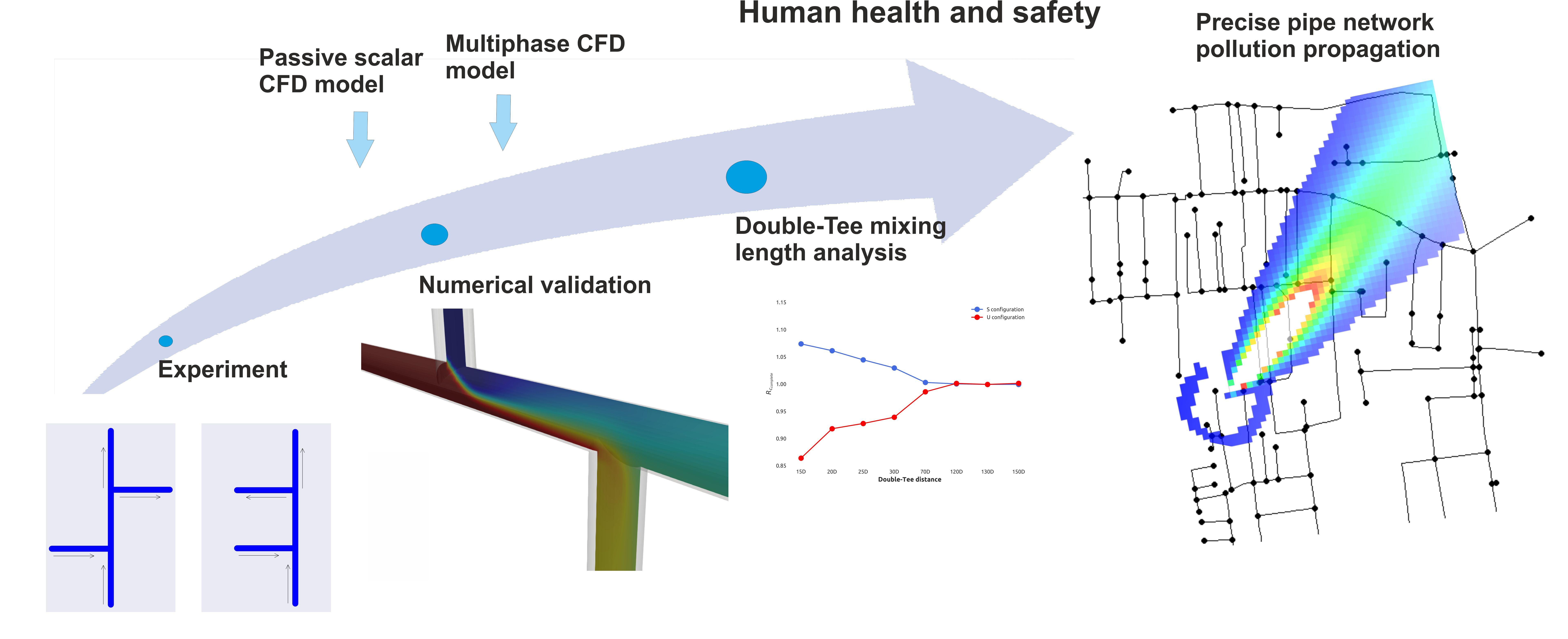
Investigated distances between Tee junctions are 5.6D, 10D, 15D, 20D, 25D, 30D, 70D, 120D, 130D and 150D for both configurations. The distance between Tee junctions refers to the centerline distance of pipe 2 and pipe 4. The 5.6D distance is the smallest one that could be physically constructed due to tees design. Investigated inlet flows range from 0.08 l/s to 0.43 l/s (Reynolds numbers range from 6000 to 30,000 in inlet pipes) and are regulated with valves to obtain different inlet volume flow ratios. Flow ratios considered for distances 5.6D, 10D and 15D at inlet branches are 3:1, 2:1, 1:1, 1:2 and 3:1 while for all other distances the ratio is 1:1. Flow at the outlet is regulated to be the same in both pipes for all experimental runs. A complete overview of the experiment can be seen in Table 1 and a schematic of the experiment can be seen in Figure 2.
2.2. Measurement Procedure and Apparatus
Distilled water used in the experiment is produced in the faculty laboratory from the tap water acquired from the water supply network. To account for the possible changes in water quality in the water supply network, the conductivity of both distilled and tap water is measured before every experimental run. Samples of mixture for conductivity measurement are taken at both outlet pipes after the distance of 40D. The temperature of both tap and distilled water is kept the same before every run to ensure that no additional effects would enhance the mixing behavior due to thermal diffusivity. Every measurement is repeated twice to make sure the results were consistent.
Since both distilled and tap water have a different initial electrical conductivity, the amount of mixing is determined by measuring the electrical conductivity of the mixture (S/cm) using an analog conductivity measuring cell (TetraCon 325 manufactured by WTW/Xylem Inc., Weilheim, Germany) and conductivity monitor (WTW LF 296 manufactured by WTW/Xylem Inc., Weilheim, Germany). The flow at both inlet and outlet pipes is measured with a turbine flowmeter (OMEGA FTB691A and FTB695A manufactured by OMEGA Engineering, Inc., Norwalk, CT, USA).
2.3. Numerical Modeling
Two different numerical approaches (passive scalar and multiphase) in a double-Tee pipe junctions mixing modeling are performed using OpenFOAM to further investigate the CFD as a viable tool in mixing phenomena modeling for internal fluid flow. Both numerical models are implemented along with the steady-state (passive scalar) or transient (multiphase) isothermal 3D Reynolds-Averaged Navier–Stokes (RANS) continuity and momentum equations with the K-epsilon (k-) turbulence model. For both models, a second-order upwind scheme is used for divergence terms, while for the gradient terms the central difference scheme is used. Computational mesh used for both models is unstructured and hexa-dominant. In the course of numerical mesh sensitivity analysis a range of mesh sizes from 70,000 to 2 million elements is tested depending on the geometry size for each case. Detailed mesh independence test diagrams for each case (configuration S) are given in the supplementary material (Figure S1). Therefore, the adequate mesh size was found for each case and adopted following the concentration convergence values criterion of 10.
Both models depend on the turbulent diffusion parameter which is defined as:
where refers to molecular diffusivity which is defined as m/s [18], is the turbulent Schmidt number and is the kinematic turbulent viscosity calculated from the turbulent kinetic energy k and turbulent dissipation [19]:
where is the default k- model constant equal to 0.09.
It has been shown that the values of the turbulent Schmidt number are problem specific [20] and greatly dependent on the local flow conditions. Even for a specific problem there is a range of feasible values of when using RANS turbulent models [21,22]. For RANS turbulence models values of for double-Tee junction with 2.5D distance have been reported in range between 0.001 and 0.01 and for 5D between 0.01 and 0.1 [23] while for a cross junction configuration, a number of 0.135 yielded the best agreement with experimental results [9], showing uncertainty in turbulent Schmidt number determination as given by different authors. It was reported that the Schmidt number is significantly different for RANS and LES turbulence models and that for LES models its value is 0.7 [24]. In this study, the Schmidt number is taken 0.5 for both passive scalar and multiphase models as it produced the best agreement between CFD model and experiment for all distances and all flow ratios on both U and S configurations.
2.3.1. Passive Scalar Model
In this approach an additional 3D advection-diffusion equation is solved with the isothermal steady-state RANS/k- model. It has been shown in previous studies [9,13,23] that this approach gives relatively good agreement with the experimental results. The model is defined as:
where c is a dimensionless scalar defined as 0 for distilled water and 1 for tap water as it represents the tracer, refers to turbulent diffusivity defined in Equation (1) and v is the advection velocity vector. Physically, Equation (3) can be interpreted as an additional transport of a scalar quantity c by the fluid flow. Since this approach models steady flow, it is less computationally expensive than the multiphase model (Section 2.3.2). In this study, the additional Equation (3) is implemented into the steady-state OpenFOAM solver SimpleFoam. Boundary conditions for velocity are Dirichlet boundary conditions (DBC) and the values at the inlet and outlet of pipes is defined to be the same as the experimental values. The no-slip boundary condition is used at the pipe walls. The Neumann boundary condition (NBC) is assigned for pressure p at the inlet of both pipes and at the pipe wall while at the outlets it is defined as zero to obtain a positive gradient. The dimensionless scalar c is defined as 1 at the inlet of pipe 1 (Figure 1) and 0 at the inlet of pipe 2, while the NBC is set at the outlets and pipe wall. Turbulence model variables k and are estimated [19] and assigned at the inlets and NBC set at the outlet. Turbulence wall functions are defined at the pipe walls. Boundary condition types for all variables being solved are summarized in Table 2.
2.3.2. Multiphase Model
The multiphase model approach is fundamentally transient and it is coupled with the transient RANS/k- model. This approach models the mixing of two miscible fluids and it can be considered to be an extension of the volume of fluid method [25] with an added diffusion term. The validated OpenFOAM solver twoLiquidMixingFoam [26,27,28] for two incompressible fluids is used and the 3D model is defined as:
where is the cell fraction of one fluid or phase. The cell phase fraction is connected to the RANS model via density as:
where is the density of the fluid which corresponds to the phase fraction , while is the density that corresponds to the second fluid with phase fraction . The computed density in Equation (6) should not be considered to be a real density of fluid but a density of the mixture of phases that occupy a cell in the finite volume framework. RANS model uses density in the momentum conservation equation. The phase is equal to 1 and represented tap water while distilled water phase is defined as 0. Any value between 1 and 0 describes a mixture and it can be also interpreted as a percentage of how much of which fluid is present in a cell. Equation (4) can be interpreted as an advection-diffusion equation for the phase . Being transient, this approach is more computationally expensive than the passive scalar model (Section 2.3.1).
3. Results and Discussion
3.1. Experimental Results
To validate the experimental results, S configuration results are first compared with results from previous cross junction mixing studies [8,9] showing that the obtained results are in line with referenced authors and logically bounded between the complete (upper boundary of mixing where concentrations at outlet pipes are the same) and bulk (lower boundary of mixing where instabilities and diffusion of fluid interfaces are ignored) mixing line [11], as shown in Figure 3. For clarity reasons, Figure 3 and Figure 4 show the results for double-Tee junction distances 5.6D, 10D and 15D only while all the other results for longer distances are presented separately in Section 3.1.1. Both referenced studies conducted an investigation of mixing in a cross junction which can be considered to be S configuration where the distance between two Tee junctions is zero. In Figure 3 the relationship between the inlet flow ratio and normalized conductivity of tracer at pipe 3 outlet is presented. Inlet flow ratio is defined as:
where is the flow of tap water in pipe 1 and is the flow of distilled water in pipe 2. The branch outlet to main inlet pipe conductivity ratio at pipe 4 outlet is calculated as:
where is measured conductivity of mixture at pipe 4 outlet and measured conductivity of tap water at inlet of pipe 1.
Even though the results are still in the area between bulk mixing and complete mixing line it can be observed in Figure 3 that as the distance between double-Tee junctions increases a level of mixing increases as well. Figure 3 shows the relationship of cross junction to double-Tee junction mixing results. Higher degree of mixing in double-Tee junction is expected since there is enough pipe length for two inlet streams to properly mix with a greater influence of turbulent diffusion, unlike in the cross junction case where distance between junctions does not exist and the streams are merely touching, which makes the mixing behavior move toward the bulk mixing line as seen in the data from previous studies. It can also be observed in Figure 3 that it is possible to determine the EPANET-BAM mixing parameter s (used in = + s( [11]) for double Tee mixing modeling by observing the experimental results e.g., for inlet flow ratio equal to 1 and a Tee distance of 10D, a recommended value of mixing parameter s reads 0.88. Same as for results from previous research [8,9], it can be observed that for different inlet flow ratios , the recommended mixing parameter s changes, i.e., with increase in flow ratio, the value of s increases. While the relationship between distance and the degree of mixing is obvious, complete mixing is still not achieved with the junction distance of 15D.
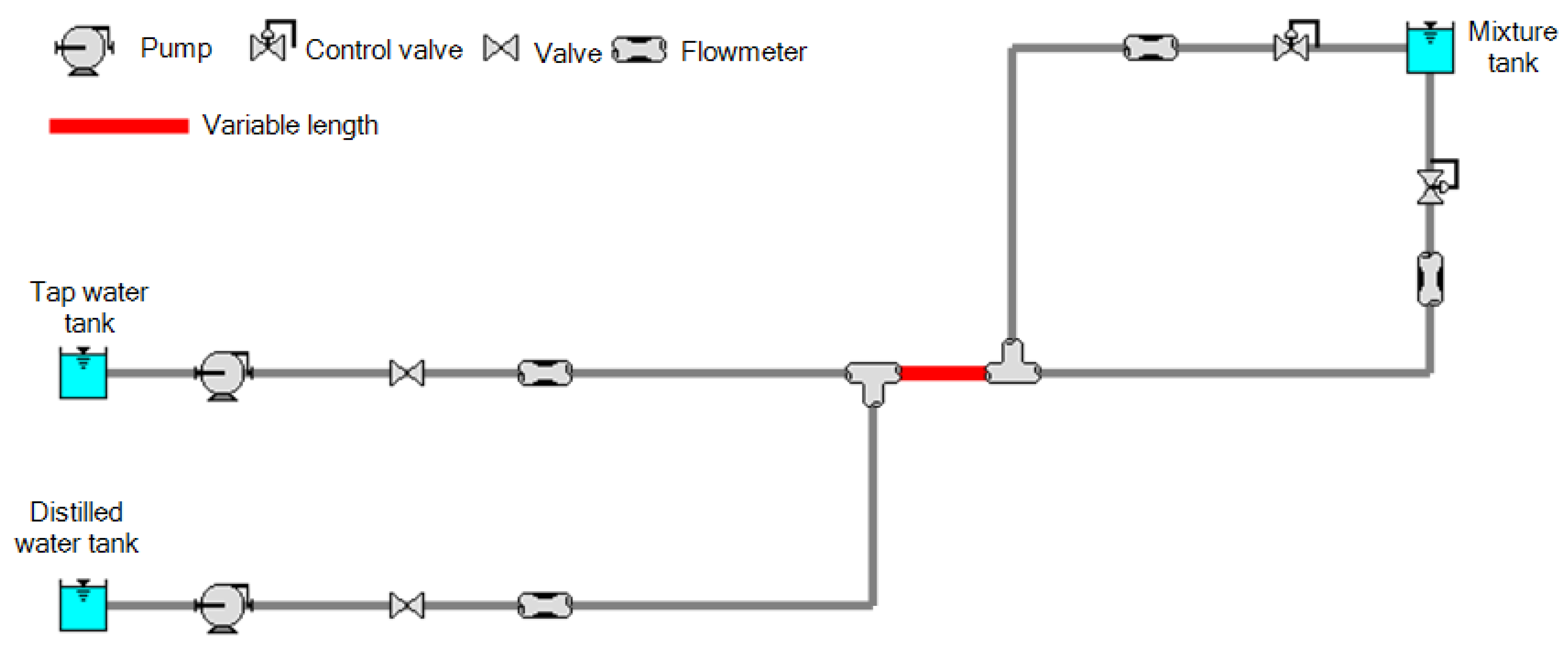
To further investigate mixing behavior both S and U configuration are compared with the experimental results from a previous study [16] where investigation of distance of Tee junctions was considered for 2.5D, 5D and 10D. The focus is on the area around the complete mixing line seen in Figure 3. The normalized main pipe inlet flow is defined as:
and branch inlet conductivity is normalized as:
where is the electrical conductivity of distilled water at inlet of pipe 2. Relation between the normalized branch inlet conductivity ratio at pipe 4 outlet and normalized main pipe inlet flow for both S and U configuration is presented in Figure 4.
It can be seen that for both configurations experimental results fall into the same region as in the previous study [16]. Configuration S results are above the complete mixing line while for the U configuration results fall below the line. In the S configuration case the tap water flow at the inlet of the main pipe 1 is dominant since the values are above the complete mixing line but for the U configuration, the clean flow of distilled water from the inlet of pipe 2 makes the greater impact since the values of the normalized concentration are in the lower region. It can be seen in both experiments that the assumption of complete mixing for Tee-junction distance of 10D is not valid (for most inlet flow ratios). Further investigations of complete mixing are conducted and results shown in the next chapter.
3.1.1. Complete Mixing
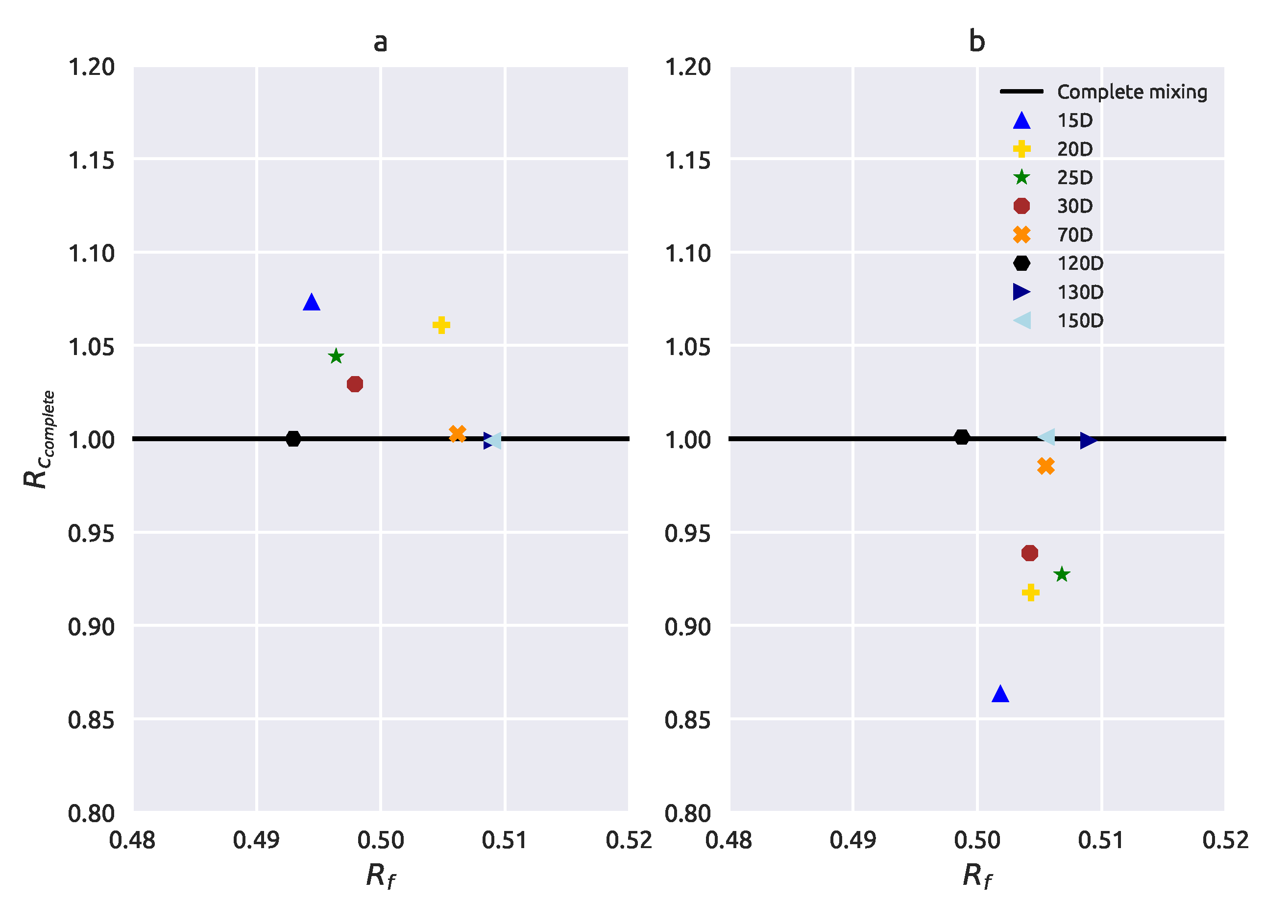
Influence of the double-Tee junction distance on complete mixing is analyzed for identical flow rates in all inlet and outlet branches and distances of 20D, 25D, 30D, 70D, 120D, 130D and 150D. In order to better visualize the behavior of mixing near the complete mixing line, the outlet conductivity ratio is defined as:
where is the measured conductivity on the pipe 3 outlet. It can be seen in Figure 5 how outlet conductivity ratio values are moving toward the complete mixing line for both pipe configurations but from the opposite sides and are mirrored in terms of the double-Tee distances’ sequence.
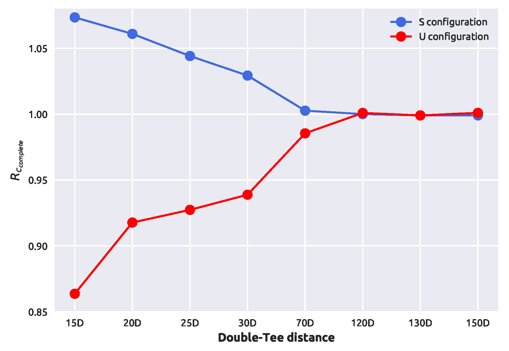
The double-Tee distance at which the complete mixing occurs in 99% and 98% magnitude for the S and U configurations respectively is 70D, while the complete mixing is achieved slightly before the 120D distance. A graph of complete mixing convergence can be seen in Figure 6. Measured mixture conductivity values at pipe outlets for both configurations, all inlet flow ratios and Tee distances can be found in supplementary material.
3.2. CFD Results
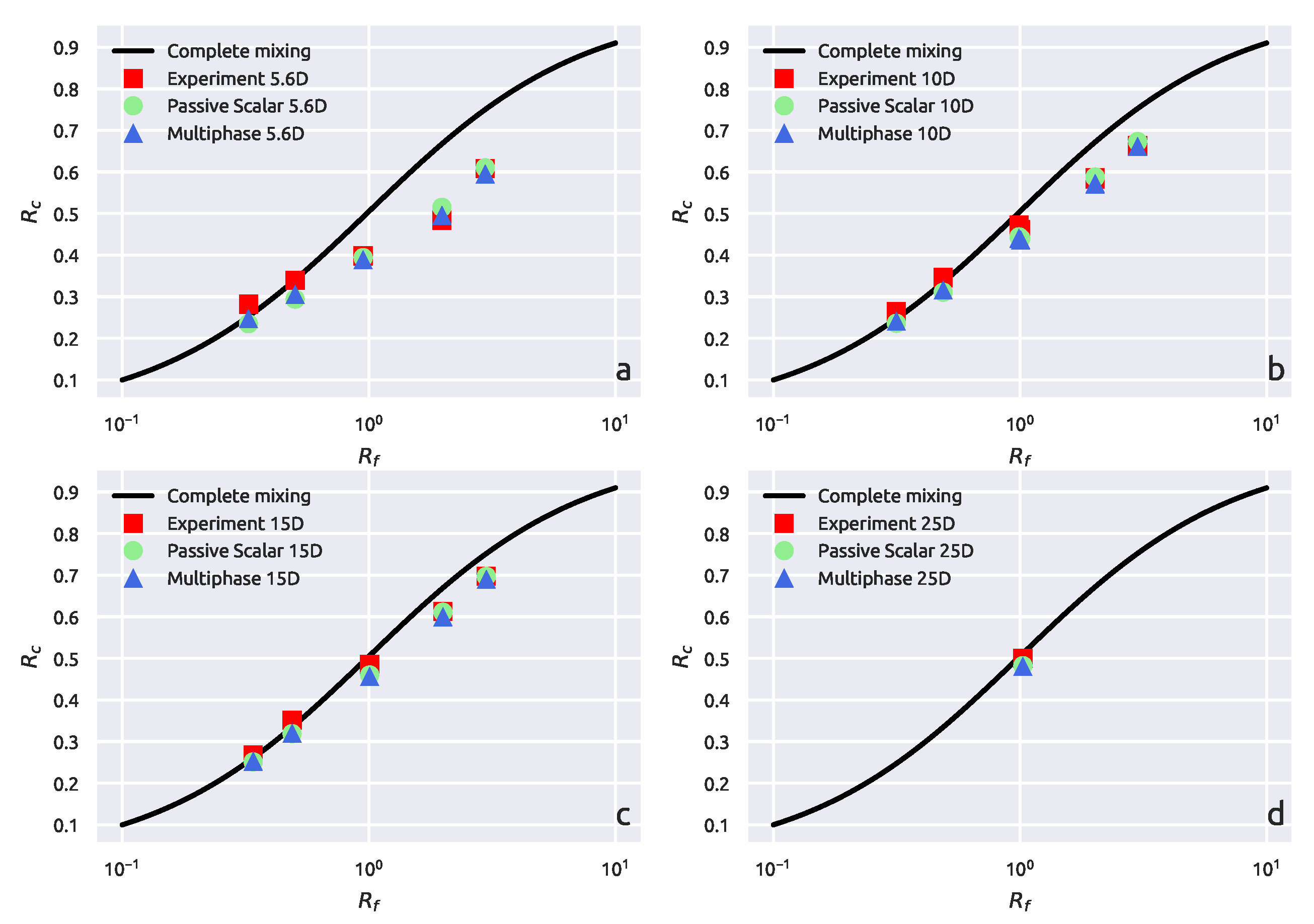
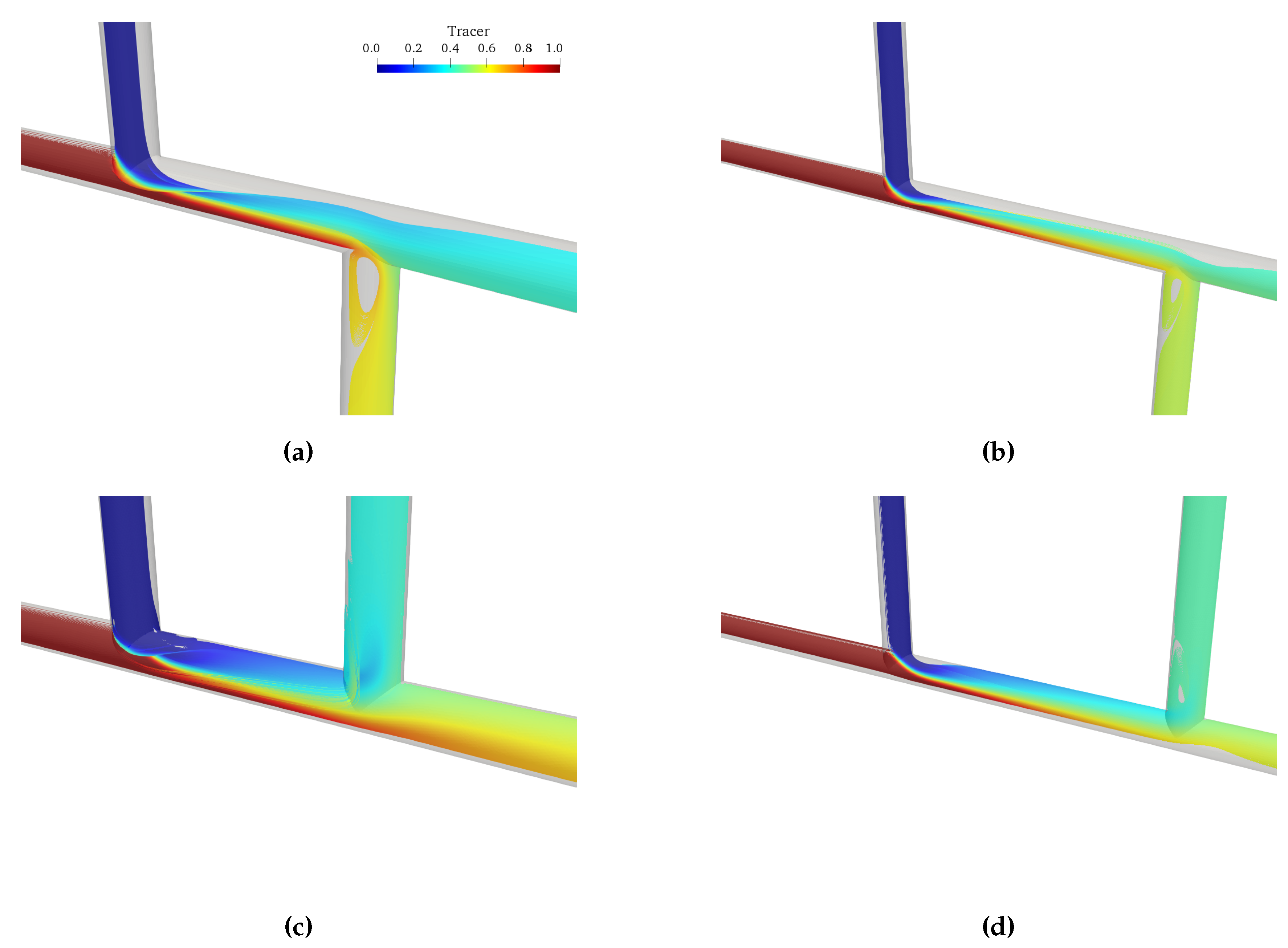
The CFD analysis is done on both pipe configurations for all inlet flow ratios for distances of 5.6D, 10D, and 15D and compared with experimental results. Additionally, a comparison is also done on the distance of 25D but only for the inlet flow ratio of 1:1 since that is the only experimental result available for that distance. Normalization is done the same way as in Equation (8) and the results for the S configuration can be seen in Figure 7 while the results for the U configuration are presented in Figure 8. Both passive scalar and multiphase model show a good agreement with the experimental results which proves that CFD is a necessary tool in mixing phenomena modeling. The essential part of the correct modeling is to properly calibrate the turbulent Schmidt number presented in Equation (1) and both models show a major dependence on it. Through the calibration procedure, it is proved that the same value of Schmidt number, 0.5, can be used for all geometries and flow ratios to obtain good results. This value is different from values found in previous studies, as discussed in Section 2.3, which shows that specific problems, in this case mixing, have a specific Schmidt number which needs to be experimentally calibrated. Since in all cases both models exhibit equal result quality, it can be concluded that using a multiphase model for this particular problem of mixing in two double-Tee junctions is not necessary since it is computationally more expensive than the passive scalar model. A visualization of CFD mixing simulation results of tracer streamlines for both configurations can be seen in Figure 9 and numerical study results can be found in supplementary material.
Computation is done using the supercomputer resources at the Center for Advanced Computing and Modeling of the University of Rijeka. Transient multiphase model took about 2 s of simulation time (on average) to converge to a steady-state solution which is an hour and a half (on average) of computation time on supercomputer Intel E7 fat node with 128 threads while the steady-state passive scalar model converged (on average) in 10 min on the same hardware (after 3000 iterations).
4. Conclusions
This paper brings new experimental data to the pipe mixing analysis investigation. The mixing behavior in two different double Tee-junction configurations (S and U) was investigated both experimentally and numerically. Experimental results were compared to experimental data available in previous studies which confirmed that the assumption of complete mixing in cross junctions is not valid and causes inaccuracy in pipe network pollution propagation modeling. Also, due to the fact that distance of 10D between the Tee junctions is usually taken as a distance after which complete mixing occurs, experimental investigations were conducted for greater distances between Tee junctions and complete mixing was observed for distances slightly before the 120D.
Numerical simulations comparing two different numerical approaches are validated by experimental work in this paper. Numerical analysis was conducted using passive scalar and multiphase models in OpenFOAM. It was shown that both models are greatly dependent on the turbulent Schmidt number through the turbulent diffusion parameter (as seen in Equation (1)). Both models, passive scalar and multiphase model exhibited excellent fitting with the experiment. Comparison of two numerical approaches showed that steady-state passive scalar model was absolutely sufficient for this type of mixing phenomenon analysis because it brought similar results with only the fraction of computational cost compared to the transient multiphase model.
Numerical simulations provide greater insight into the nature of mixing and helps to define correction parameters for complete mixing in engineering numerical software used for pipe network simulations. In this sense, the importance of the Schmidt number is emphasized. Calibration of the numerical model was performed using the Schmidt number showing the significance of this number in mixing phenomenon numerical simulations control. The Schmidt number value of 0.5 was obtained and experimentally confirmed to be valid for the whole range of inlet flow ratios, Reynolds number values, pipe configurations, and Tee-junction distances. This numerical model fitting effort should prove as a useful tool when simulating other distances and other flow ratios, and it can be used to better represent incomplete mixing behavior since, due to experiment cost, available data is usually limited.
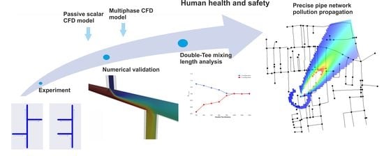
In future work, in order to contribute to the pipe network pollution propagation problem which is an environmental topic of the great importance for human health and for safety reasons, analysis of double-Tee pipe junctions (as primary building blocks of any realistic pipe network system), its integration in realistic pipe network via machine learning algorithms and simulation of different pollution propagation scenarios should be conducted in order to usefully apply this scientific research and use it as an efficient environmental analysis tool.
Supplementary Materials
The following are available online at https://www.mdpi.com/2073-4441/11/6/1198/s1, Table S1: Experimental results for S configuration, Table S2: Experimental results for U configuration, Table S3: Experimental and numerical results for S configuration, Table S4: Experimental and numerical results for U configuration, Figure S1: Mesh independence test.
Author Contributions
Conceptualization, L.G. and L.K.; Data curation, L.G. and I.L.; Formal analysis, L.G., L.K. and I.L.; Investigation, L.G. and I.L.; Methodology, L.K., I.L. and Z.Č.; Project administration, L.K. and Z.Č.; Resources, L.K.; Software, L.G.; Supervision, L.K. and Z.Č.; Validation, L.G. and I.L.; Visualization, L.G.; Writing—original draft, L.G., L.K. and I.L.; Writing—review & editing, L.G., L.K., I.L. and Z.Č.
Funding
This work has been supported in part by Ministry of Science, Education and Sports of the Republic of Croatia under the project Research Infrastructure for Campus-based Laboratories at the University of Rijeka, number RC.2.2.06-0001. Project has been co-funded from the European Fund for Regional Development (ERDF). The authors would like to thank the graduate and undergraduate students for their participation in the experiment.
Conflicts of Interest
The authors declare no conflict of interest.
References
- Rossman, L.A. EPANET 2: Users Manual; United States Environmental Protection Agency: Cincinnati, OH, USA, 2000.
- Ostfeld, A.; Uber, J.G.; Salomons, E.; Berry, J.W.; Hart, W.E.; Phillips, C.A.; Watson, J.P.; Dorini, G.; Jonkergouw, P.; Kapelan, Z.; et al. The battle of the water sensor networks (BWSN): A design challenge for engineers and algorithms. J. Water Res. Plan. Manag. 2008, 134, 556–568. [Google Scholar] [CrossRef]
- Wang, H.; Harrison, K.W. Improving efficiency of the Bayesian approach to water distribution contaminant source characterization with support vector regression. J. Water Res. Plan. Manag. 2012, 140, 3–11. [Google Scholar] [CrossRef]
- Hu, C.; Zhao, J.; Yan, X.; Zeng, D.; Guo, S. A MapReduce based Parallel Niche Genetic Algorithm for contaminant source identification in water distribution network. Ad Hoc Netw. 2015, 35, 116–126. [Google Scholar] [CrossRef]
- Seth, A.; Klise, K.A.; Siirola, J.D.; Haxton, T.; Laird, C.D. Testing contamination source identification methods for water distribution networks. J. Water Res. Plan. Manag. 2016, 142, 04016001. [Google Scholar] [CrossRef]
- Kranjčević, L.; Čavrak, M.; Šestan, M. Contamination source detection in water distribution networks. Eng. Rev. 2010, 30, 11–25. [Google Scholar]
- Yan, X.; Zhao, J.; Hu, C.; Zeng, D. Multimodal optimization problem in contamination source determination of water supply networks. Swarm Evolut. Comput. 2017. [Google Scholar] [CrossRef]
- McKenna, S.A.; Orear, L.; Wright, J. Experimental determination of solute mixing in pipe joints. In Proceedings of the World Environmental and Water Resources Congress 2007: Restoring Our Natural Habitat, Tampa, FL, USA, 15–19 May 2007; pp. 1–11. [Google Scholar]
- Romero-Gomez, P.; Choi, C.; van Bloemen Waanders, B.; McKenna, S. Transport phenomena at intersections of pressurized pipe systems. In Proceedings of the Water Distribution Systems Analysis Symposium, Cincinnati, OH, USA, 27–30 August 2006; pp. 1–20. [Google Scholar]
- Austin, R.; Waanders, B.V.B.; McKenna, S.; Choi, C. Mixing at cross junctions in water distribution systems. II: Experimental study. J. Water Res. Plan. Manag. 2008, 134, 295–302. [Google Scholar] [CrossRef]
- Ho, C.K. Solute mixing models for water-distribution pipe networks. J. Hydraul. Eng. 2008, 134, 1236–1244. [Google Scholar] [CrossRef]
- Ho, C.K.; O’Rear, L., Jr. Evaluation of solute mixing in water distribution pipe junctions. J. Am. Water Works Assoc. 2009, 101, 116–127. [Google Scholar] [CrossRef]
- Shao, Y.; Yang, Y.J.; Jiang, L.; Yu, T.; Shen, C. Experimental testing and modeling analysis of solute mixing at water distribution pipe junctions. Water Res. 2014, 56, 133–147. [Google Scholar] [CrossRef] [PubMed]
- Yu, T.; Tao, L.; Shao, Y.; Zhang, T. Experimental study of solute mixing at double-Tee junctions in water distribution systems. Water Sci. Technol. Water Supply 2015, 15, 474–482. [Google Scholar] [CrossRef]
- Yu, T.; Qiu, H.; Yang, J.; Shao, Y.; Tao, L. Mixing at double-Tee junctions with unequal pipe sizes in water distribution systems. Water Sci. Technol. Water Supply 2016, 16, 1595–1602. [Google Scholar] [CrossRef]
- Song, I.; Romero-Gomez, P.; Andrade, M.A.; Mondaca, M.; Choi, C.Y. Mixing at junctions in water distribution systems: an experimental study. Urban Water J. 2018, 15, 32–38. [Google Scholar] [CrossRef]
- Jasak, H.; Jemcov, A.; Tukovic, Z. OpenFOAM: A C++ library for complex physics simulations. In Proceedings of the International Workshop on Coupled Methods in Numerical Dynamics, Dubrovnik, Croatia, 19–21 September 2007; Volume 1000, pp. 1–20. [Google Scholar]
- Mills, R. Self-diffusion in normal and heavy water in the range 1–45. deg. J. Phys. Chem. 1973, 77, 685–688. [Google Scholar] [CrossRef]
- Launder, B.E.; Spalding, D.B. The numerical computation of turbulent flows. In Numerical Prediction of Flow, Heat Transfer, Turbulence and Combustion; Elsevier: Amsterdam, The Netherlands, 1983; pp. 96–116. [Google Scholar]
- Gualtieri, C.; Angeloudis, A.; Bombardelli, F.; Jha, S.; Stoesser, T. On the values for the turbulent Schmidt number in environmental flows. Fluids 2017, 2, 17. [Google Scholar] [CrossRef]
- Valero, D.; Bung, D.B. Sensitivity of turbulent Schmidt number and turbulence model to simulations of jets in crossflow. Environ. Model. Softw. 2016, 82, 218–228. [Google Scholar] [CrossRef]
- Valero, D.; Bung, D.; Oertel, M. Turbulent dispersion in bounded horizontal jets: RANS capabilities and physical modeling comparison. In Sustainable Hydraulics in the Era of Global Change, Proceedings of the 4th IAHR Europe Congress, Liege, Belgium, 27–29 July 2016; CRC Press: Boca Raton, FL, USA, 2016; p. 49. [Google Scholar]
- Ho, C.K.; Wright, J.L.; McKenna, S.A.; Orear, L., Jr. Contaminant Mixing at Pipe Joints: Comparison between Laboratory Flow Experiments and Computational Fluid Dynamics Models; Technical Report; Sandia National Lab. (SNL-NM): Albuquerque, NM, USA, 2006. [Google Scholar]
- Webb, S.W.; van Bloemen Waanders, B.G. High fidelity computational fluid dynamics for mixing in water distribution systems. In Proceedings of the Eight Water Distribution Systems Analysis Symposium, Cincinnati, OH, USA, 27–30 August 2006; pp. 1–15. [Google Scholar]
- Hirt, C.W.; Nichols, B.D. Volume of fluid (VOF) method for the dynamics of free boundaries. J. Comput. Phys. 1981, 39, 201–225. [Google Scholar] [CrossRef]
- Zhang, S.; Jiang, B.; Law, A.W.K.; Zhao, B. Large eddy simulations of 45 inclined dense jets. Environ. Fluid Mech. 2016, 16, 101–121. [Google Scholar] [CrossRef]
- Jiang, M.; Law, A.W.K.; Lai, A.C. Turbulence characteristics of 45 inclined dense jets. Environ. Fluid Mech. 2019, 19, 27–54. [Google Scholar] [CrossRef]
- Krpan, R.; Končar, B. Simulation of turbulent wake at mixing of two confined horizontal flows. Sci. Technol. Nucl. Install. 2018, 2018, 5240361. [Google Scholar] [CrossRef]
Figure 1.
Two different experimental configurations with variable distance between two Tee junctions where inlet pipes are labeled as 1 and 2 and outlet pipes as 3 and 4. D represents distilled water, T represents tap water and M represents mixture: (a) Distilled water inlet and mixture outlet branch on opposite sides (configuration S). (b) Distilled water inlet and mixture outlet branch on the same side (configuration U).

Figure 2.
Complete experimental setup schematic with the S configuration.

Figure 3.
Experimental results for the S configuration—relationship between branch outlet to main inlet pipe conductivity ratio and inlet flow ratio compared with previous studies [8,9] of cross junction mixing results. Dashed lines represent the value of mixing parameter s used in EPANET-BAM [12].

Figure 4.
S and U configuration experimental results—normalized branch inlet conductivity ratio to normalized main pipe inlet flow compared with the previous study [16] and shown in relation to the complete mixing line: (a) Configuration S, (b) Configuration U.
Figure 4.
S and U configuration experimental results—normalized branch inlet conductivity ratio to normalized main pipe inlet flow compared with the previous study [16] and shown in relation to the complete mixing line: (a) Configuration S, (b) Configuration U.

Figure 5.
Influence of Tee junctions distance on complete mixing—the relationship between inlet flow ratio and outlet conductivity ratio : (a) Configuration S (b) Configuration U.
Figure 5.
Influence of Tee junctions distance on complete mixing—the relationship between inlet flow ratio and outlet conductivity ratio : (a) Configuration S (b) Configuration U.

Figure 6.
Relation between the outlet conductivity ratio and Tee-junction distance.

Figure 7.
S pipe configuration—comparison of experimental results with passive scalar and multiphase model results for different Tee-junction distances: (a) 5.6D, (b) 10D, (c) 15D, (d) 25D.
Figure 7.
S pipe configuration—comparison of experimental results with passive scalar and multiphase model results for different Tee-junction distances: (a) 5.6D, (b) 10D, (c) 15D, (d) 25D.

Figure 8.
U pipe configuration - comparison of experimental results with passive scalar and multiphase model results for different Tee-junction distances: (a) 5.6D, (b) 10D, (c) 15D, (d) 25D.
Figure 8.
U pipe configuration - comparison of experimental results with passive scalar and multiphase model results for different Tee-junction distances: (a) 5.6D, (b) 10D, (c) 15D, (d) 25D.

Figure 9.
CFD tracer streamlines visualization for identical inlet flow ratio: (a) Configuration S, 5.6D, (b) Configuration S, 10D, (c) Configuration U, 5.6D, (d) Configuration U, 10D.
Figure 9.
CFD tracer streamlines visualization for identical inlet flow ratio: (a) Configuration S, 5.6D, (b) Configuration S, 10D, (c) Configuration U, 5.6D, (d) Configuration U, 10D.


Table 1.
Experimental setup data overview for S and U configuration.
| Parameter | Value | Unit |
|---|---|---|
| Internal pipe diameter (D) | 18 | (mm) |
| Inlet pipes length | 20D | (-) |
| Outlet pipes length | 40D | (-) |
| Tee distances | 5.6D, 10D, 15D, 20D, 25D, 30D, 70D, 120D, 130D, 150D | (-) |
| Inlet flow range | 0.08–0.43 | (l/s) |
| Reynolds number range | 6000–30,000 | (-) |
| Inlet flow ratios (5.6D, 10D, 15D) | 3:1, 2:1, 1:1, 1:2, 3:1 | (-) |
| Inlet flow ratios (20D, 25D, 30D, 70D, 120D, 130D, 150D) | 1:1 | (-) |
Note: (-) - dimensionless.
Table 2.
Boundary conditions summary for the passive scalar model (n represents the normal vector) and refers to the wall shear stress.
Table 2.
Boundary conditions summary for the passive scalar model (n represents the normal vector) and refers to the wall shear stress.
| Variable | Inlets | Outlets | Pipe Walls |
|---|---|---|---|
| p | p | ||
| c | c | ||
| k | k | ||
Table 3.
Boundary conditions summary for the multiphase model.
| Variable | Inlets | Outlets | Pipe Wall |
|---|---|---|---|
| p | p | ||
| k | k | ||
© 2019 by the authors. Licensee MDPI, Basel, Switzerland. This article is an open access article distributed under the terms and conditions of the Creative Commons Attribution (CC BY) license (http://creativecommons.org/licenses/by/4.0/).
Share and Cite
MDPI and ACS Style
Grbčić, L.; Kranjčević, L.; Lučin, I.; Čarija, Z. Experimental and Numerical Investigation of Mixing Phenomena in Double-Tee Junctions. Water 2019, 11, 1198. https://doi.org/10.3390/w11061198
AMA Style
Grbčić L, Kranjčević L, Lučin I, Čarija Z. Experimental and Numerical Investigation of Mixing Phenomena in Double-Tee Junctions. Water. 2019; 11(6):1198. https://doi.org/10.3390/w11061198
Chicago/Turabian StyleGrbčić, Luka, Lado Kranjčević, Ivana Lučin, and Zoran Čarija. 2019. "Experimental and Numerical Investigation of Mixing Phenomena in Double-Tee Junctions" Water 11, no. 6: 1198. https://doi.org/10.3390/w11061198
Note that from the first issue of 2016, this journal uses article numbers instead of page numbers. See further details here.