Attribution Analysis of Dry Season Runoff in the Lhasa River Using an Extended Hydrological Sensitivity Method and a Hydrological Model


1
State Key Laboratory Water Resources and Hydropower Engineering Science, Wuhan University, Wuhan 430072, China
2
China Institute of Water Resources and Hydropower Research, Beijing 100038, China
*
Author to whom correspondence should be addressed.
Water 2019, 11(6), 1187; https://doi.org/10.3390/w11061187
Submission received: 13 May 2019
/
Revised: 1 June 2019
/
Accepted: 5 June 2019
/
Published: 7 June 2019
(This article belongs to the Special Issue Advances in Hydrogeology: Trend, Model, Methodology and Concepts)
Abstract
:In this study, a coupled water–energy balance equation at an arbitrary time scale was proposed as an extension of the Budyko hypothesis. The second mixed partial derivative was selected to represent the magnitude of the interaction. The extended hydrological sensitivity method was used to quantitatively evaluate the impacts of climate change, anthropogenic activities, and their interaction on dry season runoff in the Lhasa River. In addition, an ABCD model, which is a monthly hydrological model included a snowmelt module, was used to calculate the change in soil water and groundwater storage. The Mann–Kendall test, Spearman’s test, dynamic linear model (DLM), and Yamamoto’s method were used to identify trends and change points in hydro-climatic variables from 1956–2016. The results found that dry season runoff increased non-significantly over the last 61 years. Climate change, which caused an increase in dry season runoff, was the dominant factor, followed by anthropogenic activities and their interaction, which led to varying degrees of decrease. This study concluded that the methods tested here performed well in quantifying the relative impacts of climate change, anthropogenic activities, and their interaction on dry season runoff change.
1. Introduction
The Qinghai-Tibet Plateau has long been a focus of international academic concern because it is the source point of many of Asia’s largest rivers and possesses a unique high plateau climate. The Lhasa River, situated in the southeastern part of the Qinghai-Tibet Plateau, is recognized as a sensitive area with respect to global climate change and also experiences the most anthropogenic activities in Tibet [1]. In recent years, much research has focused on streamflow variability and climate change in the Lhasa River Basin (LRB) [2,3,4]. Lin et al. [5] analyzed the characteristics of annual and monthly mean runoff in the LRB from 1956–2003. They observed an increasing trend in annual runoff with two abrupt change points around 1970 and in the early 1980s. Liu et al. [6] established the correlation between discharge and temperature using correlation analysis and identified an abrupt change point for winter streamflow. However, these studies focused more on runoff characteristics at an annual scale or qualitative attribution analysis of streamflow variability, while few addressed extreme hydrological regimes such as floods or low flows in the Lhasa River Basin. As the economy and society develop, such extreme hydrological regimes, especially low flows, could lead to environmental and natural resource issues [7]. Consequences include water shortages, drinking water contamination, and more. To better understand the water cycle and water resources in the Qinghai-Tibet Plateau and promote responsible water resources development in Lhasa, analysis of Lhasa River runoff characteristics during the dry season is needed, along with identification of the possible causes of streamflow variability.
It is undeniable that climate change, intensive anthropogenic activities, and their complex interactions have led to significant changes in water cycles and streamflow variability [8,9,10]. Climate change has a direct impact on precipitation and evaporation, while anthropogenic activities can modify temporal and spatial distribution through land use change, river diversion, dam construction, and other engineering and management practices. However, quantifying the impacts of climate change and anthropogenic activities on runoff variation is still in the exploratory stages. Various methodologies—such as hydrological modeling, the time trend method, paired catchment method, and Budyko framework—have been used to investigate the impacts of climate change and anthropogenic activities on streamflow [11,12,13,14,15,16,17]. Of these, the hydrological sensitivity method based on the Budyko hypothesis has attracted more attention due to its convenience and lower data requirements [18,19]. However, this method has two basic assumptions [20]: first, changes in soil and groundwater storage are generally ignored at annual or multi-annual scales; second, the impacts of climate change and anthropogenic activities on runoff variation are independent. The first assumption limits the applicability of the Budyko method at monthly or seasonal scales, but several methods have been proposed to solve this problem [21,22]. Wang and Alimohammadi [23] suggested that effective rainfall, as the difference between rainfall and soil water storage, could be used in place of the available water supply. Therefore, calculated effective rainfall replaces rainfall in both the climate aridity index and the evaporation ratio. Recently, Han et al. [24] proposed a null-parameter formula of the storage–evapotranspiration relationship based on a simplified proportionality hypothesis. However, the attribution analysis methods used in these studies were mostly based on Budyko decomposition [25] and few studies have applied hydrological sensitivity analysis to seasonal runoff attribution. The second assumption considers the causes of runoff change including climate change and human activities, but ignores the interactions between them.
To solve the problems mentioned above, the Budyko hypothesis was first replaced by the “coupled water–energy balance equation at an arbitrary time scale” derived by Yang et al. [26]. Yang’s equation is always valid at annual or monthly scales. More interestingly, it takes the same form as the Penman equation at the daily scale and the Budyko hypothesis at the annual (or multi-annual) scale. Based on this equation, the second mixed partial derivative was then taken to represent the magnitude of the interaction between climate change and anthropogenic activities. When using the hydrological sensitivity method based on the Budyko hypothesis, a fundamental assumption is that both water storage and deep groundwater losses are negligible during both the baseline or altered periods. However, the validity of this assumption has been poorly addressed in previous studies [27]. In this study, an improved ABCD model was proposed to verify whether water storage variability between the baseline and altered periods could be ignored.
The specific objectives of this study were to: (1) explore trends and abrupt changes in dry season runoff in the Lhasa River; (2) simulate monthly runoff to assess variability in soil water and groundwater storage using an improved ABCD model; and (3) based on the results of the above two, quantify the impacts of climate change, anthropogenic activities, and their interaction on runoff using an extended hydrological sensitivity method. This is the first effort to attribute changes in runoff to climate change, anthropogenic activities, and their interaction in the LRB. Analyzing dry season runoff variability and quantifying the roles of climate change and anthropogenic activities will contribute to the study of extreme hydrology in the Lhasa River and serve as a guide for future water resource management in the LRB.
2. Methods
2.1. Preliminary Data Analysis
The observed streamflow data over the study period from the Lhasa station need to be preliminarily examined before analyzing the recent trends and abrupt changes of dry season runoff in the LRB. In this study, we take the normality and homogeneity test to ensure the validity of the observed time.
Many normality tests are widely used in hydrological time series analysis, for example, normal Q-Q plot, histogram, skewness and kurtosis test, Shapiro–Wilk test and so on [28,29]. Among these tests, the Shapiro–Wilk test [30] was used in this study to verify the normality of streamflow in the LRB. This test generates two values: W and P. The value of W is in the range from 0 to 1, and a higher W values means the acceptance of normality and a lower W values means leads to rejection. If W is equal to 1, it means that normality is totally satisfied. If the p-value is higher than the critical significance level, normality will be accepted.
The homogeneity test of the hydrometeorological time series is essential regarding the quality assurance. Several methods of testing the homogeneity of hydrometeorological time series, for example, standard normal homogeneity test, Buishand’s test, and Pettitt’s test are offered to check whether a data series has been sourced from homogeneous heterogeneous records [31,32]. In this study, Pettitt’s test was applied to check the homogeneity of streamflow records from the Lhasa station over 61 years from 1956 to 2016.
2.2. Statistical Methods
2.2.1. Trend Analysis Method
To understand existing and future water resources development in any basin, it is important to investigate trends in hydroclimatic variables. Here, the Mann–Kendall (MK) test, Spearman’s correlation test, and dynamic linear models (DLM) were used to analyze dry season runoff trends at Lhasa Hydrological Station. Among these methods, MK test and Spearman’s correlation test are widely used in hydrological trend analysis, while DLM model is not common. We mainly introduce DLM model below, and the introduction of MK and Spearman’s test can be referred to relevant literature [33,34].
The DLM model is a state space model [35]. The purpose of fitting and analyzing the time series is achieved by modeling the regular hidden state contained in the real observation sequence. Similar to the hidden Markov model (HMM), the hidden state of the DLM model also satisfies the Markov property. The formula is
where yt are the observations at time t, with t = 1, 2, …, n. Vector xt of length m contains the unobserved states if the system that are assumed to evolve in time according to linear system operator Gt (a m × m matrix). We observe a linear combination of the states with noise and matrix Ft (m × p) is the observation operator that transforms the model states into observations. Both observation and equations can have additive Gaussian errors with covariance Vt and Wt.
In order to build a DLM for the trend, we introduce xt with two hidden states , where is the mean level and is the change in the level from time t − 1 to time t. then Equation (1) can be rewritten as
where is Gaussian stochastic terms. In terms of the Equation (1), it then becomes
In our analysis, we will set = 0 and estimate from the observations.
A first autoregressive model (AR(1)) is used to estimate autocorrelation in the residuals. In DLM form, we simply define
Then we combine the selected individual model components into larger model evolution and observation equations by
the parameters and model states are estimated by an efficient adaptive Markov chain Monte Carlo (MCMC) algorithm by Haario et al. [36] and the Kalman filter likelihood. Seasonal components are not considered in this study due to the time series being analyzed are at an annual scale. The details of the estimation procedure can be found in [37,38] and are not covered in this article.
2.2.2. Abrupt Change Analysis
Many methods can be used to detect abrupt hydro-climatic changes, such as the moving T test, Yamamoto’s method, the Mann–Kendall test, and Crammer’s method. In this paper, MK [39,40] and Yamamoto methods [41] were selected due to their user-friendly properties, such as no probability distribution limits for data and simple calculation.
In the MK method, the element in the time series is presumed to be random and independent to each other [42]. In order to reduce the impact of serial correlation on the MK test, pre-whitening by Von Storch [43] was used to remove serial correlation from time series as
where Xt is the raw time series, r1 is the lag 1 serial correlation coefficient of sample data, which can be estimated from sample data by an autocorrelation function as given in the work of Salas et al. [44].
Under the null hypothesis of no trend, the time series of variables has no change, the time series could be regarded as x1, x2, …, xn. mi is computed as the number of xi in the series whose values exceeded xj ()). The test statistic is calculated as
The expected value and variance of could be shown as
We define
Applying the method to the inverse series, we could obtain the series of as
The terms of the constitute curve UF, and the terms of the constitute curve UB. If the intersection of the two curves (UF and UB) was within the confidence interval while UF was outside the confidence interval, that point was considered to be the start of mutation [45].
Yamamoto method is used to test the significant difference for means between two random sample series, which was proposed based on the t-test. Given a reference year, the signal-to-noise ratio (SNR) is defined as
where , and , are the mean and variance for the data series before and after the reference year.
The MK test was first used to identify change points for runoff, precipitation, and potential evapotranspiration. If multiple change points were detected in the same time series, Yamamoto’s method was then used to test the significance of those change points. Only the significant abrupt change that exceeded the confidence interval in Yamamoto’s method was confirmed as the possible change point. Finally, the significant change points were combined with anthropogenic activities in the LRB. Change point detection was used to divide the monthly runoff series into the baseline and altered periods.
2.3. Coupled Water–Energy Balance Equation at an Arbitrary Time Scale
Yang et al. [26] developed an analytical coupled water–energy balance equation at an arbitrary time scale to estimate actual evapotranspiration over different time scales. The equation can be expressed as
where E is actual evapotranspiration, E0 is potential evapotranspiration, P is precipitation, I is the external water supply for a basin, S is soil moisture at the beginning of the month, w is a parameter representing basin characteristics, and C is a constant for a particular basin.
We assume that I equals zero when there is no irrigation or inter-regional water transportation. Available water is expressed as P-DS [21], and C is ignored at monthly or daily scales. Equation (1) can then be further transformed into
where DS represents the change in total water stored in the basin, including the change in soil water storage and groundwater storage. Equation (2) has a similar form to the Choudhury-Yang equation [46,47].
2.4. Extended Hydrological Sensitivity Method
For a natural basin, the water balance equation can be expressed as
where R is runoff and P is precipitation.
Substituting Equation (2) into Equation (3), we obtain the mathematical expression of R with respect to P, E0, DS, and w
Based on average monthly precipitation , monthly streamflow , average monthly potential evapotranspiration , and average change of total stored water , the parameter w can be obtained by solving an implicit function as
where .
For a gauged basin of interest, the first step of runoff attribution analysis using the hydrological sensitivity method is to split the historic time series into two subseries at a year before which anthropogenic activity was negligible. The years prior to this split refer to the baseline period (bp for simplicity), while the latter years refer to the altered period (ap). Then the runoff variability can be estimated as
where is mean runoff during the altered period, is mean runoff during the baseline period, is the change in runoff due to climate change only, and is the change in runoff due to anthropogenic activity only.
Based on the assumption that both soil water and groundwater storage losses are negligible during the baseline or altered periods, the change in runoff caused by climate change can be simplified as
where and are changes in P and E0 between the altered and baseline periods, respectively. Then can be solved by combining Equations (6) and (7).
This study also took the interaction between climate change and anthropogenic activities into account when calculating runoff variability, and Equation (6) becomes
Konapala et al. [48] presented a three-parameter-based streamflow elasticity model considering soil water storage variability as an extension of Equation (7), which is expressed as
where is the changes in DS between the altered and baseline periods.
In fact, Equation (22) is part of the first-order Taylor expansion of Equation (17), and we can also extend it into second-order Taylor series as follows.
For convenience, we introduce , where i = 1, 2, 3, 4 denote P, E0, DS and w, respectively. are the average respective values of P, E0, DS, and w during the baseline period. are the average respective values of P, E0, DS, and w during the altered period.
Then the second-order Taylor expansion of runoff change and its respective partial derivatives can be expressed as
where is a linear term, is a nonlinear term, is the coupled term, is a two-level Taylor Remainder. The specific formulae for each term are shown in Table 1.
Runoff change due to climate impacts can generally be regarded as the sum of the linear and nonlinear terms that quantify the impacts of precipitation and potential evapotranspiration [49]. Considering the close connection between surface water and groundwater in the LRB, the terms that quantify the impact of water storage change DS and parameter w represent runoff change due to anthropogenic activities. The remaining coupled term is runoff change due to the interaction between climate change and anthropogenic activities. Hence
where p denotes the number of climatic variables (e.g., precipitation or potential evapotranspiration). The relative impacts of climate change, anthropogenic activities, and their interaction on streamflow can be further estimated as
where , , and are the percentages of the impact of climate change, anthropogenic activities, and their interaction on runoff, respectively.
2.5. An Improved ABCD Model with a Snow Melt Module
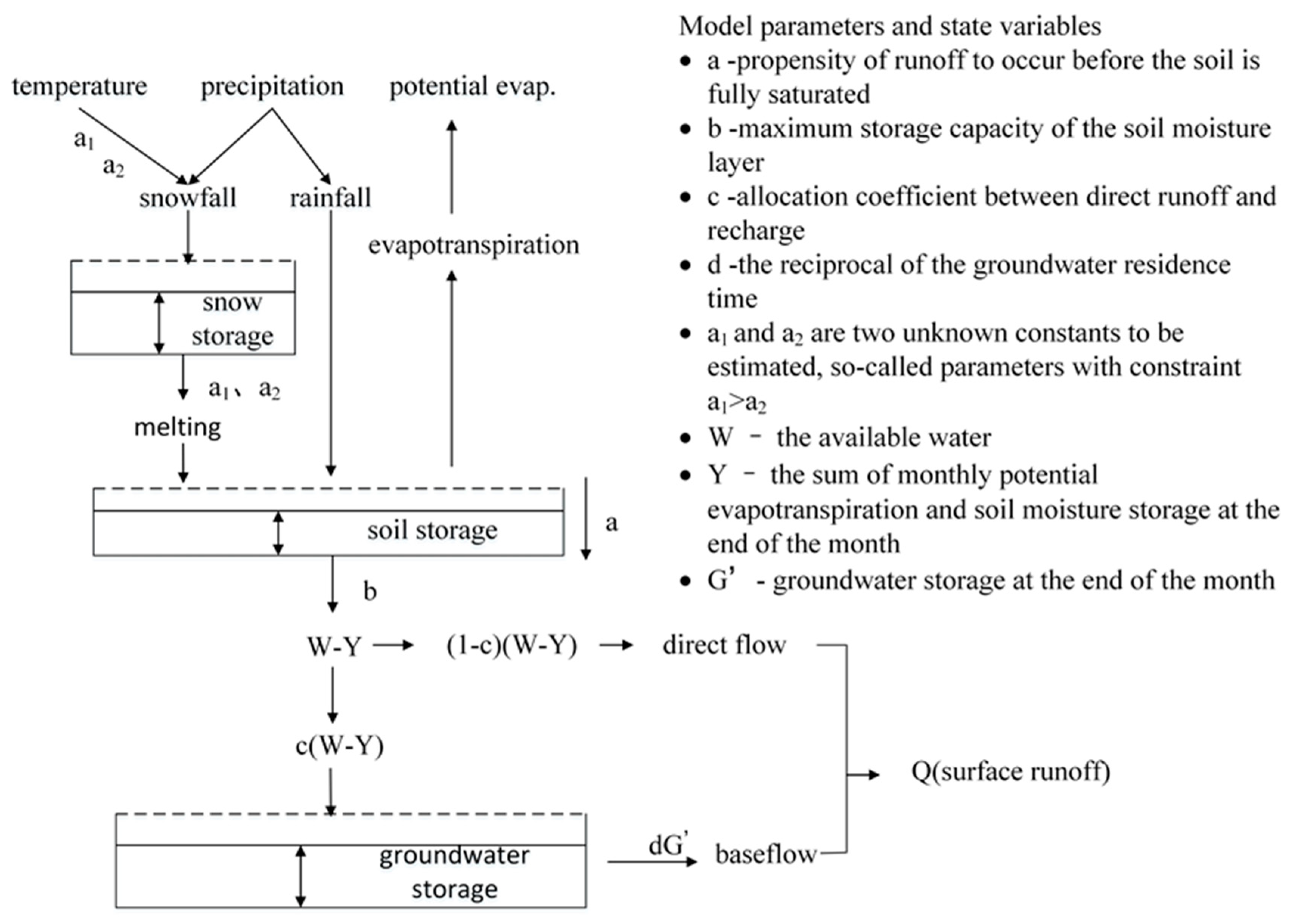
The ABCD model is a monthly hydrological model with four parameters (a, b, c, and d) developed by Thomas Jr. [50], which uses precipitation and potential evapotranspiration to simulate actual evapotranspiration, surface/subsurface runoff, and storage changes [51]. It has been widely applied as a hydro-climatologic model to investigate the response of basins to climate change and performs well in humid or arid regions [52,53]. Considering that summer and autumn snowmelt in the LRB impact the regional water cycle, the snowmelt module proposed by Xu et al. [54] was embedded into the primary ABCD model. By introducing the two parameters a1 and a2, the snowmelt module was able to describe the processes of snowfall, snow cover, and snowmelt. Figure 1 is a structural diagram of the ABCD model with the snowmelt module. Detailed information on the ABCD model and snowmelt module can be found in the relevant literature [50,54] and is not covered in this article.
2.6. Genetic Algorithm Mehtod
One of the objectives of this paper was to model inter-annual storage change by optimizing the seasonal variables. The six parameters in the ABCD model (a, b, c, d, a1, and a2) were optimized using a genetic algorithm (GA) in MATLAB. Model calibration was achieved by maximizing the Nash–Sutcliffe Efficiency (NSE) of monthly runoff, which can be expressed as
where and represent the observed and simulated values, respectively.
GA is a method for solving engineering optimization problems that is based on natural selection, the process that drives biological evolution [55,56,57]. The genetic algorithm repeatedly modifies a population of individual solutions. At each step, the genetic algorithm selects individuals at random from the current population to be parents and uses them to produce the children for the next generation. Over successive generations, the population ‘evolves’ toward an optimal solution.
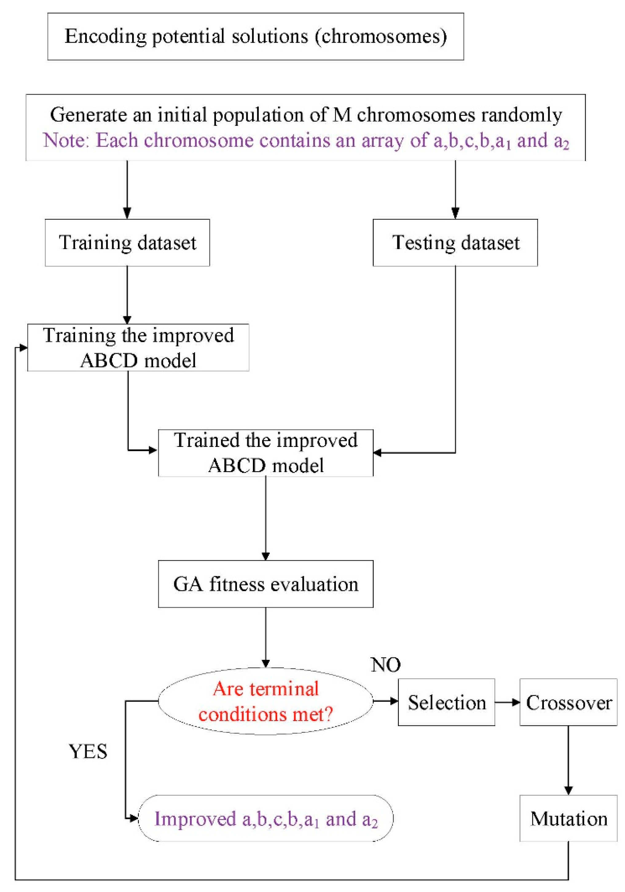
GA algorithm is utilized in order to obtain the optimum for six parameters in the improved ABCD model (a, b, c, d, a1, and a2). The flow chart in Figure 2 represents the procedure in the applied algorithm.
3. Study Area and Data Sources
3.1. Study Area Description
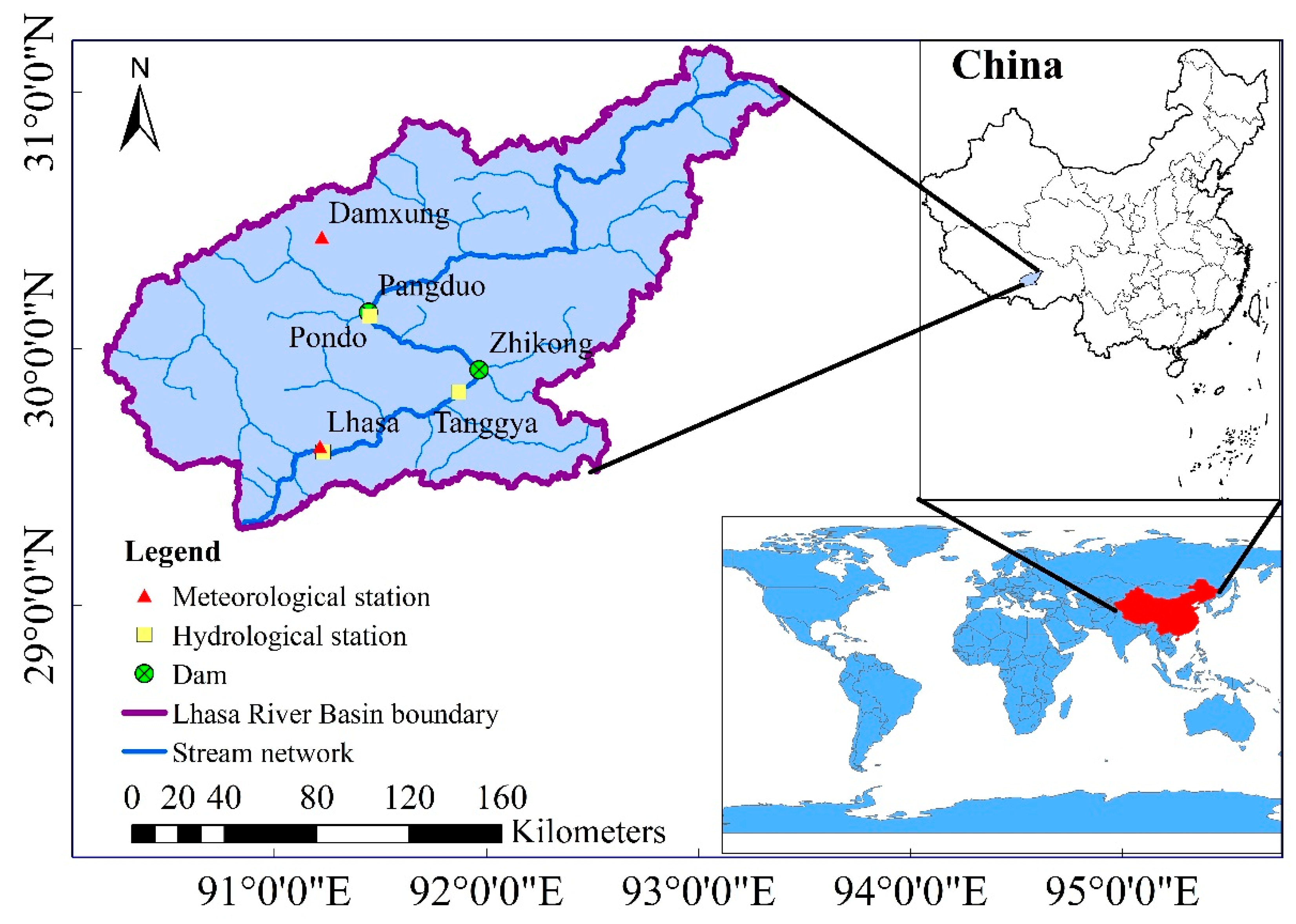
The Lhasa River is a primary branch on the left bank of the Yarlung Tsangpo River. It originates from the foothills of the Nyenchen Tanglha Mountains and flows from northeast to southwest through the Naqu area and Lhasa City. It eventually joins the Yarlung Tsangpo River near Qushui County. The study area is located in the southeastern part of the Tibet Autonomous Region, with an area of approximately 32,875 km2 and an average annual streamflow of 107.1 billion m3. Water resources in this area are abundant but also spatially and temporally heterogeneous. Precipitation is primarily concentrated from June to September and the low water period is typically from November to April. The minimum, maximum, and average runoff and precipitation for each month at the Lhasa Hydrological Station and the Lhasa Meteorological Station are given in Table 2. It is indicated from Table 2 that the river flow in May to October accounting for 87.7% of the total amount of the annual runoff, and the precipitation in June to September accounting for 89.1% of the total amount of the annual precipitation.
At present, there are three hydrological stations on the main stream: Pondo, Tanggya, and Lhasa, of which the Lhasa station has the longest time series and the most observations. The study area is the basin above Lhasa Hydrological Station, covering an area of 26,225 km2. It accounts for 79.8% of the total area of the LRB. There are three meteorological stations (Lhasa, Maizhokunggar, and Damxung) in the basin. Maizhokunggar meteorological station has a shorter observation time series and the data are not suitable for use. Damxung and Lhasa meteorological stations are distributed uniformly in the basin in the upper and lower parts of the Lhasa River, respectively. In addition, their observation conditions have not changed in recent decades. Therefore, Damxung and Lhasa meteorological stations were selected to provide the meteorological data. The geographical positions of hydrological and meteorological stations are shown in Figure 3.
3.2. Data
The data used in this study include: (1) average daily observed streamflow from the two hydrological stations (Lhasa: 1956–1968 and 1973–2016; Tanggya: 1961–2000); (2) daily precipitation, daily observation data of small/large evaporating dishes, average daily temperature from the two meteorological stations (Damxung: 1962–2016; Lhasa: 1956–2016). The hydrological data for this study were obtained from the Hydrological Bureau of Tibet Autonomous Region. Missing data for Lhasa hydrological station from 1969 to 1972 were determined by interpolation using the Tanggya streamflow data, which had a correlation coefficient of 0.98. Then daily streamflow data for Lhasa hydrological station from 1956 to 2016 were obtained. The meteorological data were collected from the China Meteorological Data Service Center (CMDC) (http://data.cma.cn). Missing data for Damxung meteorological station from 1956 to 1961 were interpolated using Lhasa meteorological station data, and the correlation coefficient was greater than 0.94.
The observed pan evaporation data were recorded using an E20 pan (an evaporimeter with a diameter of 20 cm) or E-601B pan (an evaporimeter with a diameter of 61.8 cm) depending on the external environment. In Tibet, average E20 pan and E-601B pan coefficients are 0.585 and 0.9, respectively [58]. Therefore, the potential evapotranspiration data used in this study were derived using the E20 pan or E-601B pan observations multiplied by the corresponding coefficient.
The meteorological data, monthly precipitation data, calculated potential evapotranspiration, and average temperature data were spatially averaged using Thiessen polygons to estimate values over the entire study area.
4. Results and Discussion
4.1. Preliminary Data Analysis
The Shapiro–Wilk test was applied to check the normality of streamflow, precipitation, and potential evapotranspiration data at 95% confidence level. Based on the test results W(0.75) and P(0), monthly streamflow data are considered to be non-normally distributed. The monthly precipitation and potential evaporation data series also fail to pass the Shapiro–Wilk test, with W(0.73) and P(0), and W(0.97) and P(0.1), respectively.
According to the above analysis, no observations in the monthly streamflow, precipitation, and potential evapotranspiration series fit the normality distribution very well. This means that tests which assume an underlying normality distribution are not appropriate for the trend and abrupt analysis. Instead, nonparametric methods, such as MK test and Spearman’s test, are better choices.
Pettitt’s test was applied to verify the homogeneity of the monthly streamflow, precipitation, and potential evapotranspiration data. The p-value of the three series are 1.29, 0.45, and 0.87, respectively. All the absolute value of them are higher than the typical critical value, i.e., 0.05, which indicates the three observed series are homogeneity at the 5% significance level.
4.2. Trends for Runoff, Precipitation, and Potential Evapotranspiration during the Dry Season
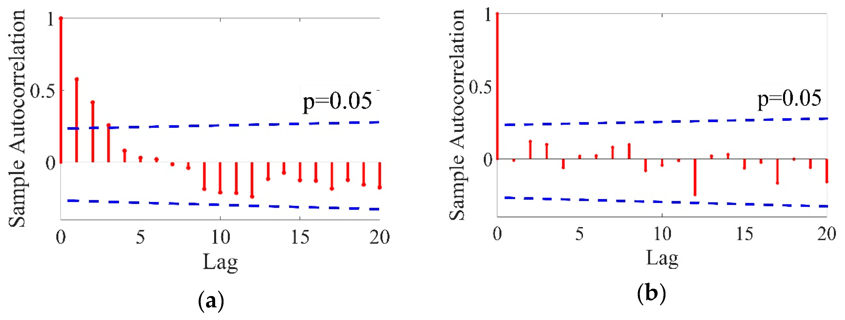
Prior to analyzing the trend by MK and Spearman’s test, we explore the correlation of the annual minimum 1-day, 3-day, 7-day, 30-day, and 90-day, dry season streamflow, precipitation, and potential evapotranspiration by calculating serial correlation coefficient. The results show that all time series, except dry season precipitation series, fail to pass the autocorrelation test. Figure 4a presents a serial coefficient under different lags for raw annual minimum 1-day flow series. The lag-one correlation coefficient (i.e., 0.58) is higher than critical value, which indicates that the assumption of data independence is not valid. Prewhitening mentioned in Section 2.2 is used to eliminate the effects of serial correlation on the MK test. As shown in Figure 4b, the lag-one correlation coefficient of ‘pre-whitened’ time series is lower than critical value, indicating that there is no autocorrelation in the pre-whitened series.
Runoff trends at the 0.05 level of significance are shown in Table 3. As seen in Table 3, there were no clear trends in the six-flow series, except for minimum one-day flow. Runoff in the Lhasa River increased non-significantly in both the dry season series and minimum 90-day flow series. In contrast, minimum 1-day, 3-day, 7-day, and 30-day flows decreased over the past 61 years, and 1d minimum runoff decreased significantly. Nevertheless, these results suggest that over shorter durations, flow decreases were more significant.
The same methods were also applied for dry season precipitation (Pdry) and potential evapotranspiration (E0,dry). Pdry and E0,dry values using the Spearman’s test were −0.45 and −0.14, respectively, while their corresponding statistics using the MK test were 3.54 and 0.89. This showed that there was a significant increasing trend for Pdry during the dry season and a non-significant decreasing trend for E0,dry over the same period. Some research [4] has confirmed increasing precipitation and almost no trend in evapotranspiration during the winter. The trend analysis results in this paper were consistent with these prior conclusions.
The DLM model without the seasonal component was fitted for observations of annual minimum 1-, 3-, 7-, 30-, 90-day flow and dry season flow separately. The variance parameters in Vt and Wt and the autocorrelation coefficient ρ used in the DLM are estimated using he MCMC simulation algorithm. The prior mean and prior standard of are 0.0005 and 200%, respectively, while the prior distribution of ρ is uniform (0, 1). Figure 5 shows the measurement series and the modeled mean background flow, μt. Overall, it is easy to see that the fits usually follow the data points very accurately. A continuous decay of flow is evident in annual minimum 1-, 3-, 7-, and 30-day flow series. The change is most visible at shorter durations. The mean value in annual minimum 90-day and dry season flow has risen from the 1956–2016. These results agree well with those obtained by MK test and Spearman’s test.
4.3. Change Point Identification of Hydro-Climatic Variables
Figure 6a and 6b shows the abrupt changes in precipitation and potential evapotranspiration identified from the dry season time series using the MK test at a significance level of 0.05. Figure 6a shows that an abrupt change in precipitation occurred during the dry season from 1970–1980. As shown in Figure 6b, there was no clear change point in dry season potential evapotranspiration.
The MK test was also used to detect change points for low water extremes related to daily, weekly, monthly, and seasonal cycles. An abrupt change occurred in 1970 for the 1-, 3-, and 7-day annual minimum time series (shown in Figure 6c,e), and two change points occurred in the 1970s and 1980s for 30- and 90-day annual minimum time series (shown in Figure 6f,g), where 1970 was a non-significant change point. Figure 6h shows that five abrupt changes in average dry season runoff occurred between 1970 and 1990. Considering the abrupt change in precipitation in 1970, the results indicate that shorter duration extreme low flows responded faster and more significantly to climate change. However, the change points for longer duration extreme low flows may reflect the impacts of human activities to some extent, which are gradual and build up over time. To reflect the effects of human activities, the average dry season runoff series was selected to be representative of low flow.
Streamflows and the abrupt climate change points detected by Yamamoto’s method at a significance level of 0.05 are shown in Figure 7a,b. An abrupt change occurred in 1986 for mean runoff in the dry season, and an abrupt change in mean dry season precipitation occurred in 1975. These results were consistent with the MK test results.
Because the abrupt change in dry season precipitation occurred nearly 10 years earlier than average runoff change over the same period, the change in dry season runoff in the 1980s was likely due to both climate change and anthropogenic activities rather than climate change alone. According to the relevant literature, there was low water resource development in the LRB until the 1980s. Since the implementation of basin planning in 1987, Zhikong hydropower station construction (2007), the Pondo hydropower station (2013), and the Moda Irrigation District (2011) have been developed in succession [59]. Earlier studies also observed abrupt changes in Lhasa River seasonal runoff in the 1980s [5]. Therefore, 1986 was selected as an abrupt change point for dry season runoff. The baseline and altered periods were then adjusted to be 1956–1985 and 1986–2016, respectively.
4.4. Modeling Dry Season Water Storage Change
Because initial soil water storage, groundwater storage, and snow depth must be known before the model run, the initial six years of the time series were chosen as the spin-up period to diminish the influence of the model state at the start of the model run. Monthly soil water and groundwater storage in the LRB were then simulated using parameters calibrated by Equation (30).
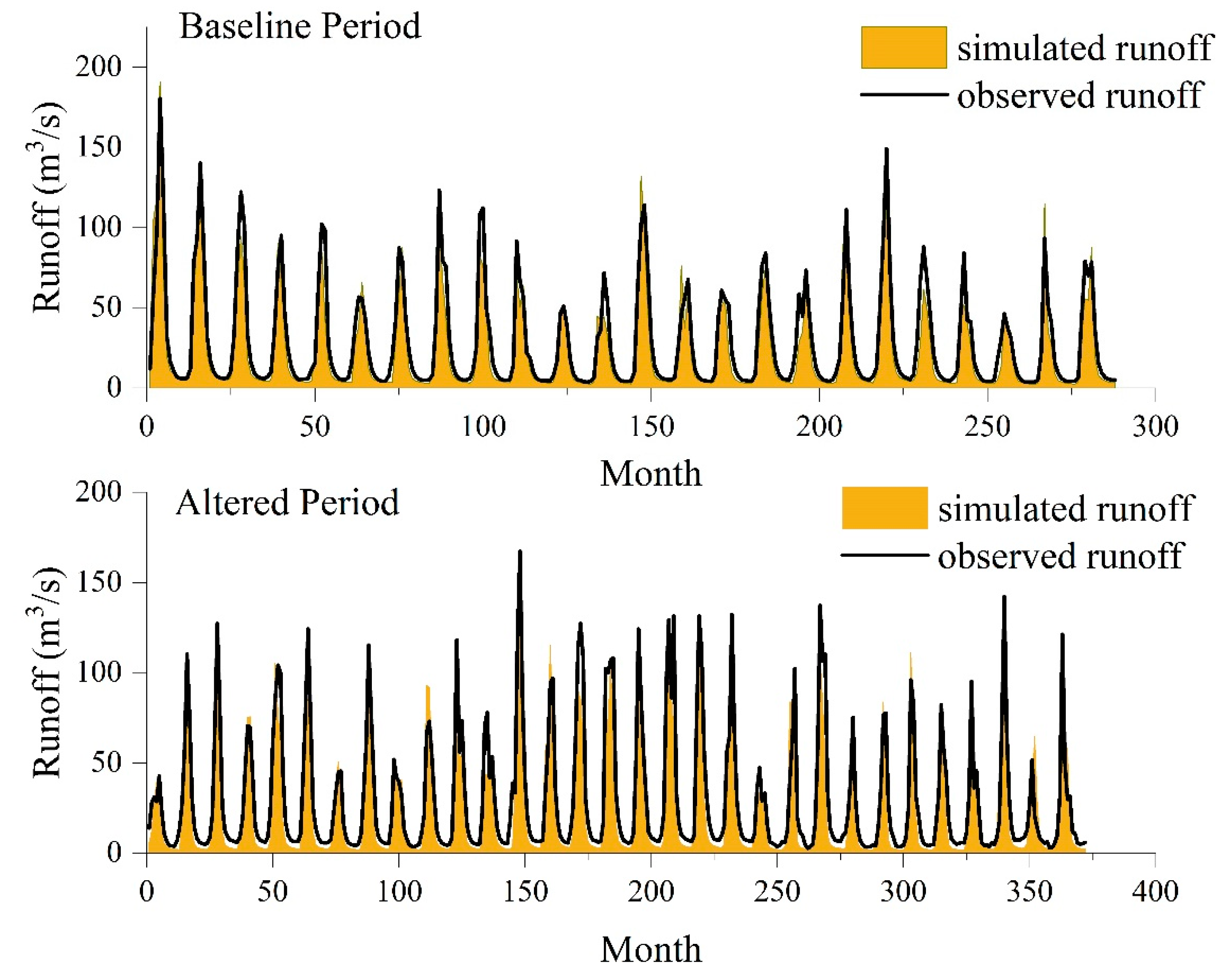
However, there was concern as to whether the parameters changed significantly before and after the change point. To verify this, the improved ABCD model was calibrated and validated based on streamflows from both the baseline and altered periods. As shown in Table 4, streamflow during the baseline period was divided into two periods: calibration (1962.5–1970.4) and validation (1970.5–1986.4). The corresponding NSE values were 0.86 and 0.84. Streamflow during the altered period was also divided into a calibration period (1986.5–1996.4) and a validation period (1996.5–2017.4), with corresponding NSE values of 0.83 and 0.81. The improved ABCD model produced good runoff simulation results for the Lhasa River. Monthly runoff simulation results at Lhasa Hydrological Station are shown in Figure 8.
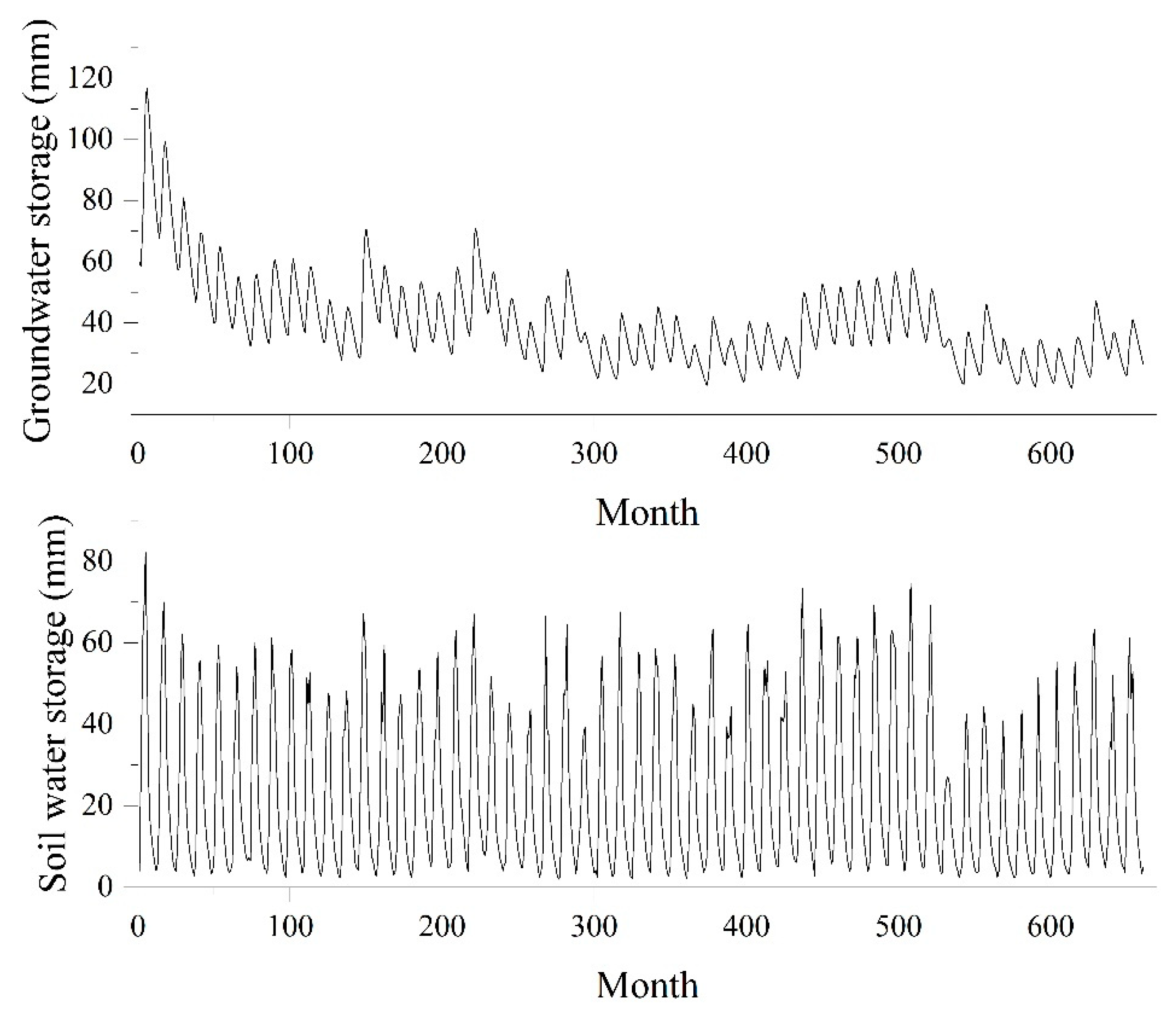
To verify the applicability of the improved ABCD model in the LRB, this paper considered the problem from two perspectives: the calibrated parameters and the runoff simulation results. From the perspective of calibrated parameters, Table 5 shows parameter ranges and corresponding calibration results. As mentioned in Section 2.5, parameter b is the upper limit of the sum of evapotranspiration and soil moisture storage in a given month. The calibration value (approximately 199.97 mm) was slightly higher than the actual value of 133 mm. Parameter c represents the proportion of streamflow derived from groundwater in a given month. The calibration value of c (0.11–0.16 mm) was about the same as the actual value (about 13%). Parameter d represents the reciprocal of average groundwater residence time. The calibration value of d was within a reasonable range considering the frequent exchange of groundwater and surface flow in the LRB [60,61]. From the perspective of the model output, simulated monthly soil water and groundwater storage are shown in Figure 9. Simulated average annual groundwater storage was 27.05mm, which was close to actual groundwater storage (about 24.7 mm). In addition, simulated soil water storage results were in good agreement with the HIMS model simulation results by Wang et al. [62]. Overall, the improved ABCD model was applicable in the LRB.
The change in dry season total stored water, DSdry, was evaluated by adding the monthly DS values in the dry season. Total dry season precipitation Pdry and runoff Rdry was used to calculate total actual evapotranspiration Edry using the water balance equation. Table 6 summarizes the differences between Pdry, Rdry, DSdry, and Edry before and after 1986. It can be observed that the absolute value of DSdry was about twice that of Pdry during both the baseline and altered periods, indicating that change in total stored water could be a significant recharge source for runoff. It was clear that neither water storage nor deep groundwater losses can be neglected during either period.
4.5. Quantitative Assessment of the Impacts of Climate Change and Anthropogenic Activities on Streamflow
Average values and variability for each variable in the baseline and altered periods are shown in Table 7. According to Equations (24)–(26) in Section 2.4, the direct impacts of P, potential evapotranspiration E0, water storage variability DS, and underlying surface w on runoff variability were quantified using the sum of corresponding linear and non-linear terms. Similarly, their interacting impacts were quantified by the sum of the coupled terms. The value of each partial derivative is summarized in Table 8. The results showed that a 10% increase in precipitation would result in a 2.30% increase in runoff, while a 10% increase in potential evapotranspiration would lead to a 13.2% decrease in runoff. For basin characteristics, a 10% increase in DS would cause a 3.2% decrease in runoff, while a 10% increase in parameter w would lead to a 6.34% decrease in runoff.
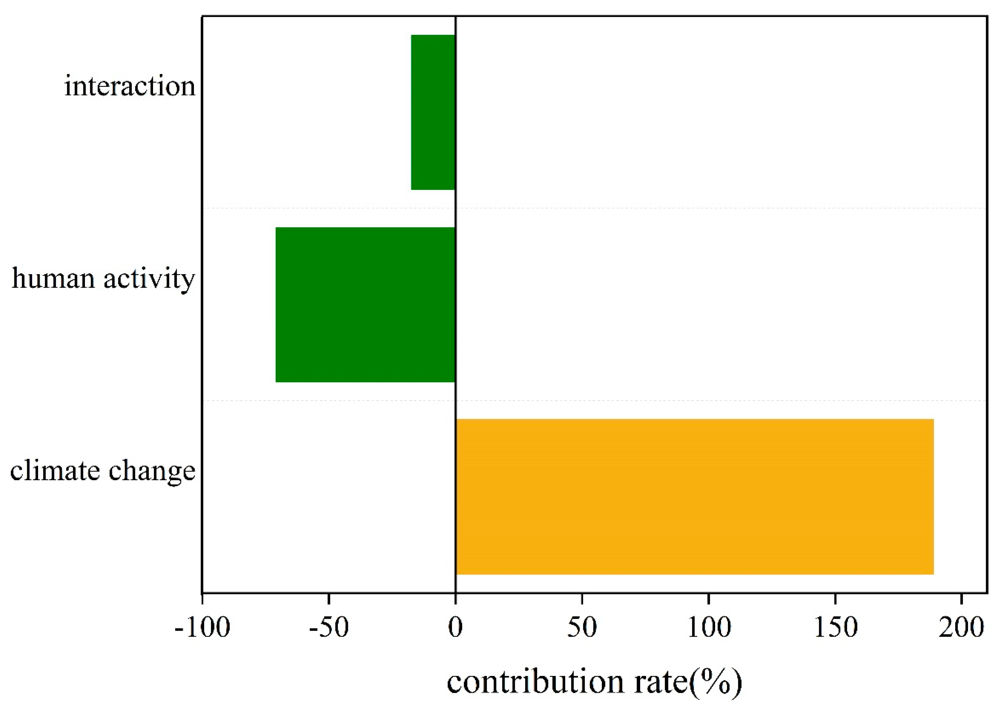
Equations (24)–(29) were used to calculate the relative contributions of climate change, anthropogenic activities, and their interaction on streamflow (shown in Figure 10). It was found that climate change with a relative contribution of 188.8% was the dominant factor affecting dry season runoff variability in the LRB. Climate change had a positive impact on dry season runoff, contributing to water supply for users and water demand in the river channel. The relative contribution of anthropogenic activities was −70.9%, indicating that it prevented the increase of runoff. This might be due to recent increases in water intake and consumption in the LRB, which countered the positive shift due to climate change to some extent. The interacting impacts also inhibited the increase in dry season runoff with a relative contribution of only −17.1%. The P and w coupled term had the largest impact of the interaction terms, which indicated that the interaction between climate change and anthropogenic activities was mainly reflected by coupled P and w. Prior literature [63] also found that climate change had a stronger impact on runoff in the LRB than anthropogenic activities, and the results of this paper were consistent with those conclusions.
4.6. Discussion
In this study, an extended hydrological sensitivity method was used to separate the impacts of climate change, anthropogenic activities, and their interaction on dry season runoff in the LRB. Compared with the current popular methods of attribution analysis [11,12,13], such as the hydrological model and Budyko framework method, the greatest advantage of the new method is that it can quantitatively determine the interaction effect. The result of the attribution analysis shows that the P and w coupled term (i.e., 0.298) had the most positive impact on the interaction. It can be explained from two perspectives. On the one hand, the changing characteristics of the underlying surface induced by anthropocentric activities, such as urbanization and afforestation, can affect regional climate cycle. On the other hand, the rainfall change also affects the underlying surface characteristics by adjusting the regional vegetation coverage in return. However, the specific mechanism of the interaction effect on streamflow is not clear and needs continued in-depth study. Another remarkable advantage of the extended hydrological sensitivity method is its applicability on monthly scales. Although many literatures [4,5,6] have provided the attribution analysis of runoff in the LRB, almost all focus on the annual scale and qualitative analysis. Besides simply function structure, the extended hydrological sensitivity method is suitable for the attribution analysis on shorter time scales and describes the contribution of different factors more accurately.
In this study, MK, Spearman’s test and DLM model was applied to investigate trends and abrupt change of annual minimum 1-day, 3-day, 7-day, 30-day, and 90-day streamflow. It is found that over shorter durations, flow decreases were more significant. Therefore, it is important to focus on low flow events (e.g., annual minimum 1-day and 3-day flow) so that the change of dry season flow can be detected early and scientifically.
With the recommended structure of the improved ABCD model for snowmelt areas, we simulated the change of soil water and groundwater in the LRB with ensured model performance on NSE. The result is close to that obtained by Wang et al. [62] who simulate streamflow of the LRB by the HIMS, VIC, and Swat models at monthly time step. The improved ABCD model has the advantage that simulate changes in soil water and groundwater simultaneously while Wang et al. obtained simulation of the soil water only. Because the water consumption in Lhasa city is highly dependent on groundwater, the simulation results of the model can provide decision-making guidance for urban development.
The extended hydrological sensitivity method and the improved ABCD model are only applied in the LRB in this study. We cannot guarantee that the basic equation, namely “Coupled water–energy balance equation at an arbitrary time scale”, has the same form in other areas. It is more likely that the form of the equation varies spatially and temporally. Therefore, the applicability of the model in other parts of the world remains to be further studied. In addition, there exits several uncertainties in the method. Firstly, the limitations due to the number and distribution of hydro-meteorological stations affect the accuracy of the simulation. Secondly, the actual evaporation was calculated using PET and pan coefficients, which increase the uncertainty of the model simulations. Finally, uncertainty of the model parameter can also influence the simulation results. Therefore, these uncertainties will affect the computational results to a certain extent.
5. Conclusions
It is important to quantify the impacts of climate change and anthropogenic activities on runoff variation of the study areas, due to the influence of human activities on water cycling processes. However, most existing sensitivity methods cannot be applied at monthly scales and ignore the interaction effect because of the basic assumptions of the Budyko hypothesis. To solve these problems, this study proposes an extended hydrological sensitivity method and an improved ABCD model to quantify the impacts of climate change, anthropogenic activities, and their interaction on dry season runoff in the LRB.
Trend and abrupt analysis can be a delicate matter and it is always challenging to give causal explanations. Hydro-climatic variable trends in the LRB were analyzed for the past 60 years. MK test, Spearman’s test, and DLM model showed that annual minimum 1-day, 3-day, 7-day, and 30-day streamflows exhibited varying levels of decrease from 1956–2016. Only the annual minimum one-day flow results tested at the 0.05 significance level. Annual minimum 90-day streamflows and mean dry season flows had non-significant increasing trends. Precipitation in the dry season significantly increased and potential evapotranspiration decreased non-significantly. Results from mutation testing for the dry season time series indicated that shorter duration low flow extremes responded faster and more significantly to climate change, while longer duration low flow extremes reflected the impacts of human activities. Combined MK and Yamomoto’s methods identified the year 1986 as an abrupt change point in dry season runoff. The monthly runoff series was then divided into two periods. Prior to 1986 (1957–1985) was regarded as the baseline period and after 1986 (1986–2016) was referred to as the altered period.
In order to simulate monthly runoff to assess variability in soil water and groundwater storage, an improved ABCD model with an embedded snowmelt module was proposed to simulate dry season runoff in the LRB. The NSE coefficient of the improved model is above 0.80. The simulation results showed that water storage variability made up a large proportion of runoff recharge, therefore neither water storage nor deep groundwater loss can be neglected in seasonal runoff change attribution.
We have shown that the extended hydrological sensitivity method is well suited for separating climate change, anthropogenic activities, and their interaction on dry season runoff in the LRB. The results showed that climate change had the greatest impacts on dry season runoff, followed by anthropogenic activities, and finally their interactions, whose relative contributions were only 1/2 and 1/11 of the former. Climate change increased runoff in the dry season, while anthropogenic activities and the interaction impact caused varying degrees of runoff reductions. The results contribute to a better understanding of the critical factors affecting the evolution of the Lhasa River runoff and can be used to serve as a guide for future water resource management in the LRB.
Author Contributions
Conceptualization: Z.W., J.C., and Y.M.; Methodology: Z.W.; Formal analysis: Z.W.; investigation: W.X.; Resources: Y.M and T.H.; Writing—original draft preparation, Z.W.; Writing—review and editing: Y.M.; Funding acquisition, T.H. All the authors have approved of the submission of this manuscript.
Funding
Financial support for this study was provided by the National Natural Science Foundation of China (91647204; 51479140).
Acknowledgments
Special thanks to Di Zhu, Hao Cai and Yue Ben for providing instructions and suggestion on this work.
Conflicts of Interest
The authors declare no conflict of interest.
References
- Wu, X.; Li, Z.; Gao, P.; Huang, C.; Hu, T. Response of the Downstream Braided Channel to Zhikong Reservoir on Lhasa River. Water 2018, 10, 1144. [Google Scholar] [CrossRef]
- Fan, J.; Sun, W.; Zhao, Y.; Xue, B.; Zuo, D.; Xu, Z. Trend Analyses of Extreme Precipitation Events in the Yarlung Zangbo River Basin, China Using a High-Resolution Precipitation Product. Sustainability 2018, 10, 1396. [Google Scholar] [CrossRef]
- Makokha, G.O.; Wang, L.; Zhou, J.; Li, X.P.; Wang, A.H.; Wang, G.P.; Kuria, D. Quantitative drought monitoring in a typical cold river basin over Tibetan Plateau: An integration of meteorological, agricultural and hydrological droughts. J. Hydrol. 2016, 543, 782–795. [Google Scholar] [CrossRef]
- You, Q.; Kang, S.; Wu, Y.; Yan, Y. Climate change over the yarlung zangbo river basin during 1961–2005. J. Geogr. Sci. 2007, 17, 409–420. [Google Scholar] [CrossRef]
- Lin, X.; Zhang, Y.; Yao, Z.; Gong, T.; Wang, H.; Chu, D.; Liu, L.; Zhang, F. The trend on runoff variations in the Lhasa River Basin. J. Geogr. Sci. 2008, 18, 95–106. [Google Scholar] [CrossRef]
- Liu, J.; Xie, J.; Gong, T.; Wang, H.; Xie, Y. Impacts of winter warming and permafrost degradation on water variability, upper Lhasa River, Tibet. Quat. Int. 2011, 244, 178–184. [Google Scholar] [CrossRef]
- Foulon, E.; Rousseau, A.N. Surface Water Quantity for Drinking Water during Low Flows—Sensitivity Assessment Solely from Climate Data. Water Resour. Manag. 2019, 33, 369–385. [Google Scholar] [CrossRef]
- Guzha, A.C.; Rufino, M.C.; Okoth, S.; Jacobs, S.; Nobrega, R. Impacts of land use and land cover change on surface runoff, discharge and low flows: Evidence from East Africa. J. Hydrol.-Reg. Stud. 2018, 15, 49–67. [Google Scholar] [CrossRef]
- Hanasaki, N.; Yoshikawa, S.; Pokhrel, Y.; Kanae, S. A global hydrological simulation to specify the sources of water used by humans. Hydrol. Earth Syst. Sci. 2018, 22, 789–817. [Google Scholar] [CrossRef] [Green Version]
- Kundzewicz, Z.W.; Kanae, S.; Seneviratne, S.I.; Handmer, J.; Nicholls, N.; Peduzzi, P.; Mechler, R.; Bouwer, L.M.; Arnell, N.; Mach, K.; et al. Flood risk and climate change: global and regional perspectives. Hydrol. Sci. J. 2014, 59, 1–28. [Google Scholar] [CrossRef]
- Mishra, V.; Cherkauer, K.A.; Niyogi, D.; Lei, M.; Pijanowski, B.C.; Ray, D.K.; Bowling, L.C.; Yang, G.X. A regional scale assessment of land use/land cover and climatic changes on water and energy cycle in the upper Midwest United States. Int. J. Climatol. 2010, 30, 2025–2044. [Google Scholar] [CrossRef] [Green Version]
- Napoli, M.; Massetti, L.; Orlandini, S. Hydrological response to land use and climate changes in a rural hilly basin in Italy. Catena 2017, 157, 1–11. [Google Scholar] [CrossRef]
- Tomer, M.D.; Schilling, K.E. A simple approach to distinguish land-use and climate-change effects on watershed hydrology. J. Hydrol. 2009, 376, 24–33. [Google Scholar] [CrossRef]
- Umar, D.A.; Ramli, M.F.; Aris, A.Z.; Jamil, N.R.; Abdulkareem, J.H. Runoff irregularities, trends, and variations in tropical semi-arid river catchment. J. Hydrol.-Reg. Stud. 2018, 19, 335–348. [Google Scholar] [CrossRef]
- Wu, J.; Miao, C.; Wang, Y.; Duan, Q.; Zhang, X. Contribution analysis of the long-term changes in seasonal runoff on the Loess Plateau, China, using eight Budyko-based methods. J. Hydrol. 2017, 545, 263–275. [Google Scholar] [CrossRef]
- Zhang, L.; Nan, Z.; Yu, W.; Zhao, Y.; Xu, Y. Comparison of baseline period choices for separating climate and land use/land cover change impacts on watershed hydrology using distributed hydrological models. Sci. Total Environ. 2018, 622–623, 1016–1028. [Google Scholar] [CrossRef] [PubMed]
- Bu, J.; Lu, C.; Niu, J.; Gao, Y. Attribution of Runoff Reduction in the Juma River Basin to Climate Variation, Direct Human Intervention, and Land Use Change. Water 2018, 10, 1775. [Google Scholar] [CrossRef]
- Li, C.; Wang, L.; Wanrui, W.; Qi, J.; Linshan, Y.; Zhang, Y.; Lei, W.; Cui, X.; Wang, P. An analytical approach to separate climate and human contributions to basin streamflow variability. J. Hydrol. 2018, 559, 30–42. [Google Scholar] [CrossRef]
- Yang, H.; Yang, D. Derivation of climate elasticity of runoff to assess the effects of climate change on annual runoff. Water Resour. Res. 2011, 47. [Google Scholar] [CrossRef]
- Dey, P.; Mishra, A. Separating the impacts of climate change and human activities on streamflow: A review of methodologies and critical assumptions. J. Hydrol. 2017, 548, 278–290. [Google Scholar] [CrossRef]
- Chen, X.; Alimohammadi, N.; Wang, D. Modeling interannual variability of seasonal evaporation and storage change based on the extended Budyko framework. Water Resour. Res. 2013, 49, 6067–6078. [Google Scholar] [CrossRef] [Green Version]
- Zhang, L.; Potter, N.; Hickel, K.; Zhang, Y.; Shao, Q. Water balance modeling over variable time scales based on the Budyko framework – Model development and testing. J. Hydrol. 2008, 360, 117–131. [Google Scholar] [CrossRef]
- Wang, D.B.; Alimohammadi, N. Responses of annual runoff, evaporation, and storage change to climate variability at the watershed scale. Water Resour. Res. 2012, 48, 5546. [Google Scholar] [CrossRef]
- Han, P.-F.; Wang, X.-S.; Istanbulluoglu, E. A Null-Parameter Formula of Storage–evapotranspiration Relationship at Catchment Scale and its Application for a New Hydrological Model. J. Geophys. Res. Atmospheres 2018, 123, 2082–2097. [Google Scholar] [CrossRef]
- Jiang, C.; Xiong, L.; Wang, D.; Liu, P.; Guo, S.; Xu, C.-Y. Separating the impacts of climate change and human activities on runoff using the Budyko-type equations with time-varying parameters. J. Hydrol. 2015, 522, 326–338. [Google Scholar] [CrossRef]
- Yang, H.; Yang, D.; Lei, Z.; Lei, H. Derivation and validation of watershed coupled water–energy balance equation at arbitrary time scale (in Chinese). J. Hydraul. Eng. 2008, 610–617. [Google Scholar]
- Wang, X. Advances in separating effects of climate variability and human activity on stream discharge: An overview. Adv. Water Resour. 2014, 71, 209–218. [Google Scholar] [CrossRef]
- Razali, N.M.; Wah, Y.B. Power comparisons of Shapiro-Wilk, Kolmogorov-Smirnov, Lilliefors and Anderson-Darling tests. J. Stat. Model. Anal. 2011, 2, 21–33. [Google Scholar]
- Kim, I.; Park, S. Likelihood ratio tests for multivariate normality. Commun. Stat. Theory Methods 2018, 47, 1923–1934. [Google Scholar] [CrossRef]
- Royston, P. Approximating the Shapiro–Wilk W-test for non-normality. Stat. Comput. 1992, 2, 117–119. [Google Scholar] [CrossRef]
- Buishand, T.A. Some methods for testing the homogeneity of rainfall records. J. Hydrol. 1982, 58, 11–27. [Google Scholar] [CrossRef]
- Pettitt, A.N. A Non-Parametric Approach to the Change-Point Problem. J. R. Stat. Soc. 1979, 28, 126–135. [Google Scholar] [CrossRef]
- Hirsch, R.M.; Slack, J.R.; Smith, R.A. Techniques of Trend Analysis for Monthly Water-Quality Data. Water Resour. Res. 1982, 18, 107–121. [Google Scholar] [CrossRef]
- Shadmani, M.; Marofi, S.; Roknian, M. Trend Analysis in Reference Evapotranspiration Using Mann–Kendall and Spearman’s Rho Tests in Arid Regions of Iran. Water Resour. Manag. 2012, 26, 211–224. [Google Scholar] [CrossRef]
- Poncela, P. Time series analysis by state space methods. Int. J. Forecast. 2004, 20, 139–141. [Google Scholar] [CrossRef]
- Haario, H.; Laine, M.; Mira, A.; Saksman, E. DRAM: Efficient adaptive MCMC. Stat. Comput. 2006, 16, 339–354. [Google Scholar] [CrossRef]
- Mikkonen, S.; Laine, M.; Mäkelä, H.M.; Gregow, H.; Tuomenvirta, H.; Lahtinen, M.; Laaksonen, A. Trends in the average temperature in Finland, 1847–2013. Stoch. Environ. Res. Risk Assess. 2015, 29, 1521–1529. [Google Scholar] [CrossRef]
- Laine, M.; Latva-Pukkila, N.; Kyrölä, E. Analysing time-varying trends in stratospheric ozone time series using the state space approach. Atmos. Chem. Phys. 2014, 14, 9707–9725. [Google Scholar] [CrossRef] [Green Version]
- Goossens, C.; Berger, A. How to Recognize an Abrupt Climatic Change? D. Reidel Publishing Company: Dordrecht, Holland, 1987. [Google Scholar]
- Mann, H.B. Nonparametric Tests against Trend. Econometrica 1945, 13, 245–259. [Google Scholar] [CrossRef]
- Yamamoto, R.; Iwashima, T.; Sanga, N.K.; Hoshiai, M. An Analysis of Climatic Jump. J. Meteorol. Soc. Jpn. 1986, 64, 273–281. [Google Scholar] [CrossRef] [Green Version]
- Yue, S.; Wang, C. Applicability of prewhitening to eliminate the influence of serial correlation on the Mann–Kendall test. WATER Resour. Res. 2002, 38. [Google Scholar] [CrossRef]
- Von Storch, H. Misuses of Statistical Analysis in Climate Research. In Analysis of Climate Variability: Applications of Statistical Techniques; von Storch, H., Navarra, A., Eds.; Springer: Berlin/Heidelberg, Germany, 1995; pp. 11–26. ISBN 978-3-662-03167-4. [Google Scholar]
- Salas, J.D. Applied Modeling of Hydrologic Time Series; Water Resources Publications: Littleton, CO, USA, 1980; Available online: https://www.researchgate.net/publication/243784685_Applied_Modeling_of_Hydrologic_Time_Series/ (accessed on 6 June 2019).
- Moraes, J.M.; Pellegrino, G.Q.; Ballester, M.V.; Martinelli, L.A.; Victoria, R.L.; Krusche, A.V. Trends in Hydrological Parameters of a Southern Brazilian Watershed and its Relation to Human Induced Changes. Water Resour. Manag. 1998, 12, 295–311. [Google Scholar] [CrossRef]
- Roderick, M.L.; Farquhar, G.D. A simple framework for relating variations in runoff to variations in climatic conditions and catchment properties. Water Resour. Res. 2011, 47. [Google Scholar] [CrossRef]
- Yang, H.; Yang, D.; Lei, Z.; Sun, F. New analytical derivation of the mean annual water–energy balance equation. Water Resour. Res. 2008, 44. [Google Scholar] [CrossRef]
- Konapala, G.; Valiya Veettil, A.; Mishra, A.K. Teleconnection between low flows and large-scale climate indices in Texas River basins. Stoch. Environ. Res. Risk Assess. 2018, 32, 2337–2350. [Google Scholar] [CrossRef]
- Ye, X.; Zhang, Q.; Liu, J.; Li, X.; Xu, C. Distinguishing the relative impacts of climate change and human activities on variation of streamflow in the Poyang Lake catchment, China. J. Hydrol. 2013, 494, 83–95. [Google Scholar] [CrossRef]
- Thomas, H.A., Jr. Improved Methods for National Water Assessment, Water Resources Contract: WR15249270; US Water Resources Council: Washington, DC, USA, 1981. Available online: https://pubs.er.usgs.gov/publication/70046351 (accessed on 6 June 2019).
- Alley, W.M. On The Treatment Of Evapotranspiration, Soil-Moisture Accounting, And Aquifer Recharge In Monthly Water-Balance Models. Water Resour. Res. 1984, 20, 1137–1149. [Google Scholar] [CrossRef]
- Pellicer Martinez, F.; Martínez Paz, J.M. Contrast and transferability of parameters of lumped water balance models in the Segura River Basin (Spain). Water Environ. J. 2015, 29, 43–50. [Google Scholar] [CrossRef]
- Shahid, M.; Cong, Z.; Zhang, D. Understanding the impacts of climate change and human activities on streamflow: A case study of the Soan River basin, Pakistan. Theor. Appl. Climatol. 2018, 134, 205–219. [Google Scholar] [CrossRef]
- Xu, C.Y.; Seibert, J.; Halldin, S.; Uppsala, U. Regional water balance modelling in the NOPEX area: Development and application of monthly water balance models. J. Hydrol. 1996, 180, 211–236. [Google Scholar] [CrossRef]
- Chang, F.-J.; Chen, L. Real-Coded Genetic Algorithm for Rule-Based Flood Control Reservoir Management. Water Resour. Manag. 1998, 12, 185–198. [Google Scholar] [CrossRef]
- Liu, P.; Li, L.; Guo, S.; Xiong, L.; Zhang, W.; Zhang, J.; Xu, C.-Y. Optimal design of seasonal flood limited water levels and its application for the Three Gorges Reservoir. J. Hydrol. 2015, 527, 1045–1053. [Google Scholar] [CrossRef]
- Farzin, S.; Singh, V.P.; Karami, H.; Farahani, N.; Ehteram, M.; Kisi, O.; Allawi, M.F.; Mohd, N.S.; El-Shafie, A. Flood Routing in River Reaches Using a Three-Parameter Muskingum Model Coupled with an Improved Bat Algorithm. Water 2018, 10, 1130. [Google Scholar] [CrossRef]
- Shi, H.; Fu, X.; Chen, J.; Wang, G.; Li, T. Spatial distribution of monthly potential evaporation over mountainous regions: case of the Lhasa River basin, China. Hydrol. Sci. J. 2014, 59, 1856–1871. [Google Scholar] [CrossRef]
- Luo, H.; Tang, Y.; Zhu, X.; Di, B.; Xu, Y. Greening trend in grassland of the Lhasa River Region on the Qinghai-Tibetan Plateau from 1982 to 2013. Rangel. J. 2016, 38, 591–603. [Google Scholar] [CrossRef]
- Ge, S.; Wu, Q.B.; Lu, N.; Jiang, G.L.; Ball, L. Groundwater in the Tibet Plateau, western China. Geophys. Res. Lett. 2008, 35. [Google Scholar] [CrossRef]
- Smith, C.; Clark, M.; Broll, G.; Ping, C.L.; Kimble, J.M.; Luo, G. Characterization of selected soils from the Lhasa region of Qinghai-Xizang Plateau, SW China. Permafr. Periglac. Process. 1999, 10, 211–222. [Google Scholar] [CrossRef]
- Wang, L.; Wang, Z.; Liu, C.; Bai, P.; Liu, X. A Flexible Framework HydroInformatic Modeling System—HIMS. Water 2018, 10, 962. [Google Scholar] [CrossRef]
- Liu, Z.; Yao, Z.; Huang, H.; Wu, S.; Liu, G. Land use and climate changes and their impacts on runoff in the Yarlung Zangbo River Basin, China. Land Degrad. Dev. 2014, 25, 203–215. [Google Scholar] [CrossRef]
Figure 1.
Water partitions in the improved ABCD model.

Figure 2.
Flowchart of the parameter optimization base on GA.

Figure 3.
Location of the Lhasa River Basin and distribution of hydro-meteorological stations.

Figure 4.
Model diagnostic on the (a) original minimum one-day flow and (b) pre-whitened minimum 1-day flow by an estimated autocorrelation function (ACF).
Figure 4.
Model diagnostic on the (a) original minimum one-day flow and (b) pre-whitened minimum 1-day flow by an estimated autocorrelation function (ACF).

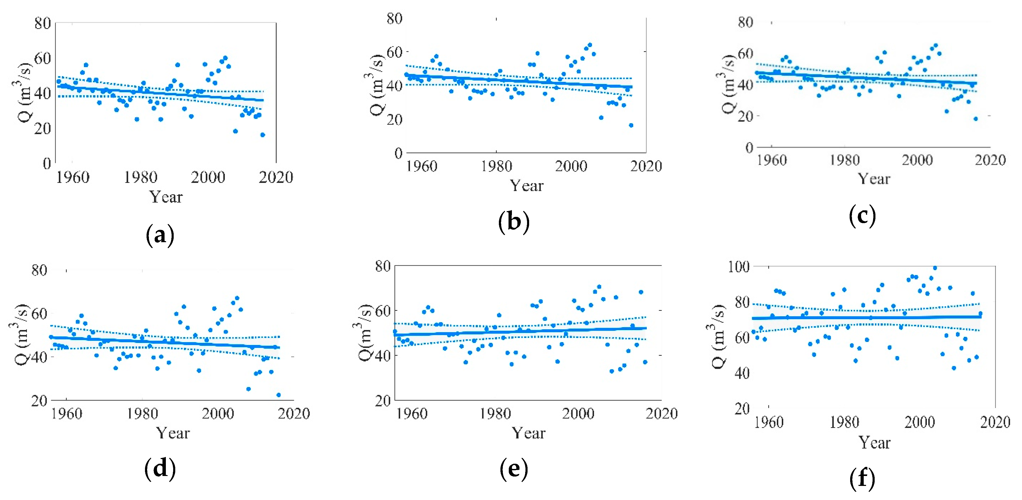
Figure 5.
DLM fit for (a) annual minimum 1-day flow runoff, (b) annual minimum 3-day flow runoff, (c) annual minimum 7-day flow runoff, (d) annual minimum 30-day flow runoff, (e) annual minimum 90-day flow runoff and (f) dry season runoff at Lhasa station. The dots are the observations used in the analysis, the solid line following the observations is the DLM fit obtained by a Kalman filter. The smooth solid line is the background level component of the model with 95% probability envelope.

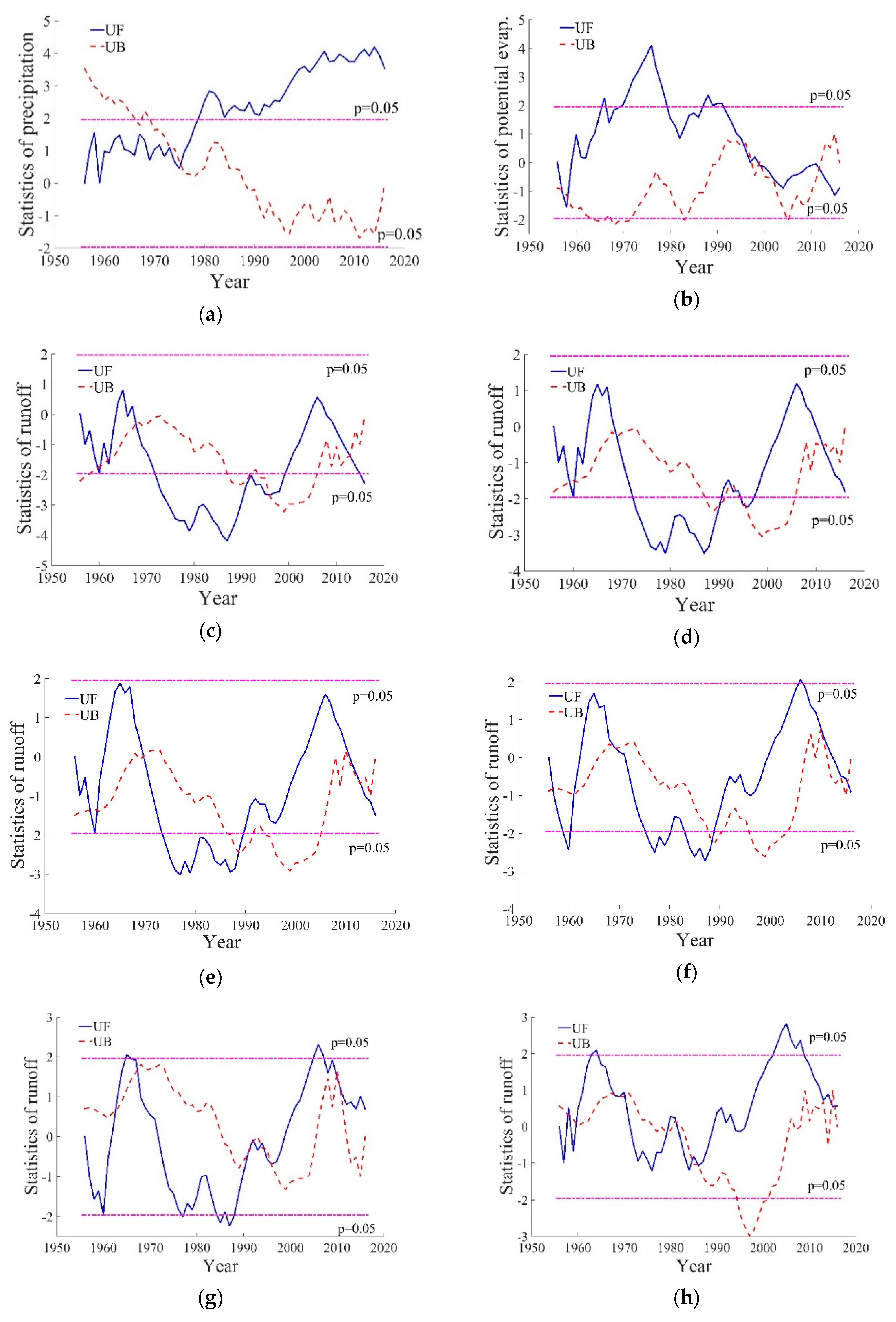
Figure 6.
Mutation analysis using MK testing: (a) precipitation, (b) potential evapotranspiration, (c) annual minimum 1-day flow runoff, (d) annual minimum 3-day flow runoff, (e) annual minimum 7-day flow runoff, (f) annual minimum 30-day flow runoff, (g) annual minimum 90-day flow runoff, and (h) dry season runoff at Lhasa station in the dry season. UF and UB were calculated using the MK test in the forward and backward directions, respectively. Horizontal dashed lines are ±95% confidence intervals.

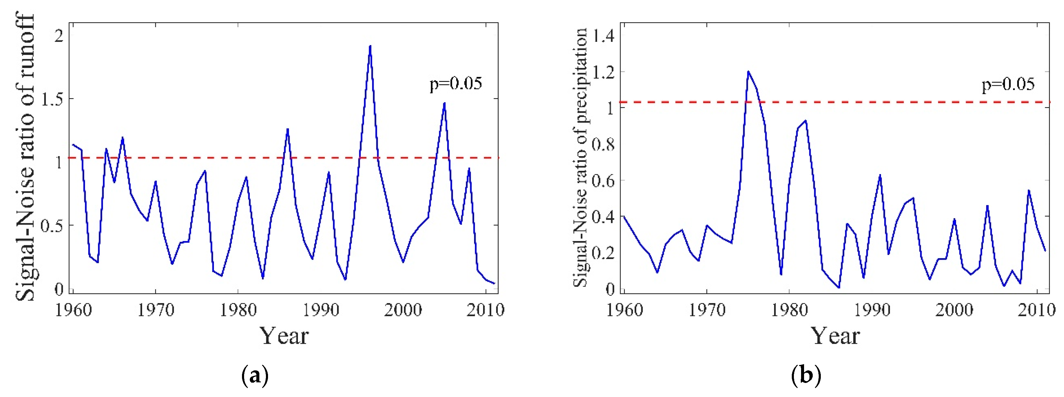
Figure 7.
Mutation analysis using Yamamoto’s method: (a) Lhasa station runoff and (b) dry season precipitation. Horizontal red lines are ±95% confidence intervals.
Figure 7.
Mutation analysis using Yamamoto’s method: (a) Lhasa station runoff and (b) dry season precipitation. Horizontal red lines are ±95% confidence intervals.

Figure 8.
Monthly runoff simulation results using the improved ABCD model at Lhasa Hydrological Station from 1962–2016. The unit of the runoff is transferred from millimeter into cubic per second (m3/s) by multiplying by the watershed area for the convenience of comparing with observed runoff.
Figure 8.
Monthly runoff simulation results using the improved ABCD model at Lhasa Hydrological Station from 1962–2016. The unit of the runoff is transferred from millimeter into cubic per second (m3/s) by multiplying by the watershed area for the convenience of comparing with observed runoff.

Figure 9.
Simulated results for monthly change in groundwater and soil water storage in the basin from 1962–2016.
Figure 9.
Simulated results for monthly change in groundwater and soil water storage in the basin from 1962–2016.

Figure 10.
Contributions of the impacts of climate change and anthropogenic activities on runoff in the Lhasa River during the dry season.
Figure 10.
Contributions of the impacts of climate change and anthropogenic activities on runoff in the Lhasa River during the dry season.


Table 1.
Expressions of different partial derivatives.
| Linear Terms | Coupled Terms | Nonlinear Terms |
|---|---|---|
Note: .
Table 2.
Runoff and precipitation for each month at the Lhasa Hydrological Station and the Lhasa Meteorological Station.
Table 2.
Runoff and precipitation for each month at the Lhasa Hydrological Station and the Lhasa Meteorological Station.
| Months | Jan. | Feb. | Mar. | Apr. | May | Jun. | Jul. | Aug. | Sept. | Oct. | Nov. | Dec. | |
|---|---|---|---|---|---|---|---|---|---|---|---|---|---|
| Runoff (m3/s) | Maximum | 85.5 | 74.3 | 78.9 | 172 | 385 | 1020 | 1370 | 1800 | 1310 | 439 | 191 | 109 |
| Minimum | 33.6 | 26 | 31.4 | 36.3 | 38.8 | 121 | 309 | 203 | 141 | 87.3 | 59.5 | 41.1 | |
| Average | 57.5 | 51.1 | 50.2 | 62.1 | 124.6 | 398.0 | 749.0 | 849.9 | 630.0 | 265.8 | 125.1 | 77.9 | |
| Precipitation (mm) | Maximum | 5.5 | 18.9 | 19.3 | 26.2 | 78.3 | 192.5 | 258.9 | 283.2 | 147.2 | 38.4 | 22.4 | 12.7 |
| Minimum | 0 | 0 | 0 | 0 | 0.2 | 5.9 | 35.3 | 29 | 11 | 0 | 0 | 0 | |
| Average | 0.6 | 1.2 | 2.5 | 6.9 | 27.2 | 76.8 | 126.8 | 130.3 | 62.0 | 8.1 | 1.2 | 0.6 | |
Table 3.
Trends for different flow components in the LRB using the Spearman’s and Mann–Kendall tests.
Table 3.
Trends for different flow components in the LRB using the Spearman’s and Mann–Kendall tests.
| Series | Number of Years | Spearman’s Test | Mann–Kendall Test | ||||
|---|---|---|---|---|---|---|---|
| r | Threshold | Tendency | z | Threshold | Tendency | ||
| Annual minimum 1-day flow | 61 | −0.28 * | 0.25 |  | −2.24 * | 1.96 | |
| Annual minimum 3-day flow | 61 | −0.23 | 0.25 | | −1.80 | 1.96 | |
| Annual minimum 7-day flow | 61 | −0.20 | 0.25 | | −1.49 | 1.96 | |
| Annual minimum 30-day flow | 61 | −0.14 | 0.25 | | −0.89 | 1.96 | |
| Annual minimum 90-day flow | 61 | 0.07 | 0.25 |  | 0.68 | 1.96 | |
| Annual dry-seasonal flow* | 61 | 0.06 | 0.25 | | 0.55 | 1.96 | |
represents a decreasing trend; represents an increasing trend. * Indicates significance at the 0.05 level. Annual dry season flow represents average seasonal runoff from November to April.Table 4.
Calibration and validation period details.
| Model | Calibration Method | Spin-Up Period | Baseline Period | Altered Period | ||
|---|---|---|---|---|---|---|
| Calibration Periods | Validation Periods | Calibration Periods | Validation Periods | |||
| Improved ABCD model | Genetic algorithm | 1956.5–1962.4 | 1962.5–1970.4 | 1970.5–1986.4 | 1986.5–1996.4 | 1996.5–2017.4 |
Table 5.
NSE values for simulated and calibrated parameter results.
| Nash-Sutcliffe Efficiency | a | b | c | d | a1 | a2 | ||
|---|---|---|---|---|---|---|---|---|
| Range | / | 0~1 | 0~200 | 0~1 | 0~20 | 0~30 | −20~20 | |
| Baseline period | Calibration periods | 0.86 | 0.64 | 199.97 | 0.16 | 0.08 | 18.4 | 9.2 |
| Validation periods | 0.84 | |||||||
| Altered period | Calibration periods | 0.83 | 0.65 | 199.98 | 0.11 | 0.07 | 14.5 | 9.5 |
| Validation periods | 0.81 | |||||||
Table 6.
Change in hydro-climatic variables (mm) in the dry season between the baseline and altered periods.
Table 6.
Change in hydro-climatic variables (mm) in the dry season between the baseline and altered periods.
| Period | Pdry | Rdry | DSdry | Edry |
|---|---|---|---|---|
| Baseline period (1962–1985) | 454.3 | 799.8 | −1026.7 | 681.1 |
| Altered period (1986–2016) | 753.9 | 1100.7 | −1057.0 | 710.3 |
| Total period (1962–2016) | 1208.2 | 1900.5 | −2083.7 | 1391.4 |
Table 7.
Change in mean monthly hydro-climatic variables due to climate change and anthropogenic activities.
Table 7.
Change in mean monthly hydro-climatic variables due to climate change and anthropogenic activities.
| Variables | Baseline Period | Altered Period | Variability |
|---|---|---|---|
| (mm/month) | 33.33 | 35.51 | 2.18 |
| (mm/month) | 18.93 | 24.32 | 5.39 |
| (mm/month) | 489.24 | 465.04 | −24.20 |
| (mm/month) | −42.78 | −34.10 | 8.68 |
| 0.44 | 0.39 | −0.05 |
Table 8.
Partial derivatives of runoff variables in the Lhasa River during the dry season.
| 3.63 | 0.40 | −5.84 | 4.02 | 0.03 | 0.01 | 0.08 |
| 0.19 | 0.04 | −0.11 | 0.298 | −0.06 | −0.03 | −0.48 |
© 2019 by the authors. Licensee MDPI, Basel, Switzerland. This article is an open access article distributed under the terms and conditions of the Creative Commons Attribution (CC BY) license (http://creativecommons.org/licenses/by/4.0/).
Share and Cite
MDPI and ACS Style
Wu, Z.; Mei, Y.; Chen, J.; Hu, T.; Xiao, W. Attribution Analysis of Dry Season Runoff in the Lhasa River Using an Extended Hydrological Sensitivity Method and a Hydrological Model. Water 2019, 11, 1187. https://doi.org/10.3390/w11061187
AMA Style
Wu Z, Mei Y, Chen J, Hu T, Xiao W. Attribution Analysis of Dry Season Runoff in the Lhasa River Using an Extended Hydrological Sensitivity Method and a Hydrological Model. Water. 2019; 11(6):1187. https://doi.org/10.3390/w11061187
Chicago/Turabian StyleWu, Zhenhui, Yadong Mei, Junhong Chen, Tiesong Hu, and Weihua Xiao. 2019. "Attribution Analysis of Dry Season Runoff in the Lhasa River Using an Extended Hydrological Sensitivity Method and a Hydrological Model" Water 11, no. 6: 1187. https://doi.org/10.3390/w11061187
Note that from the first issue of 2016, this journal uses article numbers instead of page numbers. See further details here.