Condition Assessment of Water Infrastructures: Application to Segura River Basin (Spain)
by
 , and
, and
Mario Urrea-Mallebrera
1, 
Luis Altarejos-García
2,*,
Juan García-Bermejo
2 and
and
Bartolomé Collado-López
2 1
Segura River Basin Authority, Plaza de Fontes 1, Murcia 30001, Spain
2
Technical University of Cartagena; Paseo Alfonso XIII 52, Cartagena 30203, Spain
*
Author to whom correspondence should be addressed.
Water 2019, 11(6), 1169; https://doi.org/10.3390/w11061169
Submission received: 27 April 2019
/
Revised: 3 June 2019
/
Accepted: 3 June 2019
/
Published: 4 June 2019
(This article belongs to the Special Issue Socioeconomic Indicators for Sustainable Water Management)
Abstract
:The paper deals with the condition assessment of water management infrastructures such as storage facilities, water mains and water distribution facilities. The objective is to develop a methodology able to provide a fast, simple assessment of present asset condition, that can also be used for predicting future conditions under different investment scenarios. The authors investigate the use of different methodologies to assess condition with focus on simple, indirect condition indices based on maintenance records, such as Infrastructure Value Index (IVI) and Asset Sustainability Index (ASI). The novelty of the approach presented is the development of a methodology that combines an asset inventory together with maintenance data, that can be integrated hierarchically, delivering an assessment of condition of elements, assets and groups of assets in a bottom-up fashion. The methodology has been applied to a group of water management infrastructures of the Segura River Basin in Spain. The main conclusion is that the proposed methodology allows to assess assets’ sustainability based upon past and current trends in operation and maintenance budgets, providing a baseline for planning future maintenance actions.
1. Introduction
Providing water supply for irrigation and urban use in a reliable manner begins at the raw water infrastructure level system. The mission of this system is to deliver access to water with enough quantity and quality levels, under variable hydrologic conditions, while accounting for regulatory and institutional context and operation and maintenance requirements. In addition, the system shall meet current and future, long-term, demand forecasts [1,2].
Organizations managing water infrastructures have to make decisions regarding what new infrastructures are needed, which ones should be renewed, rehabilitated or decommissioned and what maintenance activities should be performed, and when. In the case of state-owned infrastructures, provision of economic resources should be included in the State’s General Budget. The budget availability is conditioned by the existing regulatory framework, which may include provisions for the calculation of water tariffs and indications on what part of the operation and maintenance costs should be transferred to users through the tariffs [3,4,5].
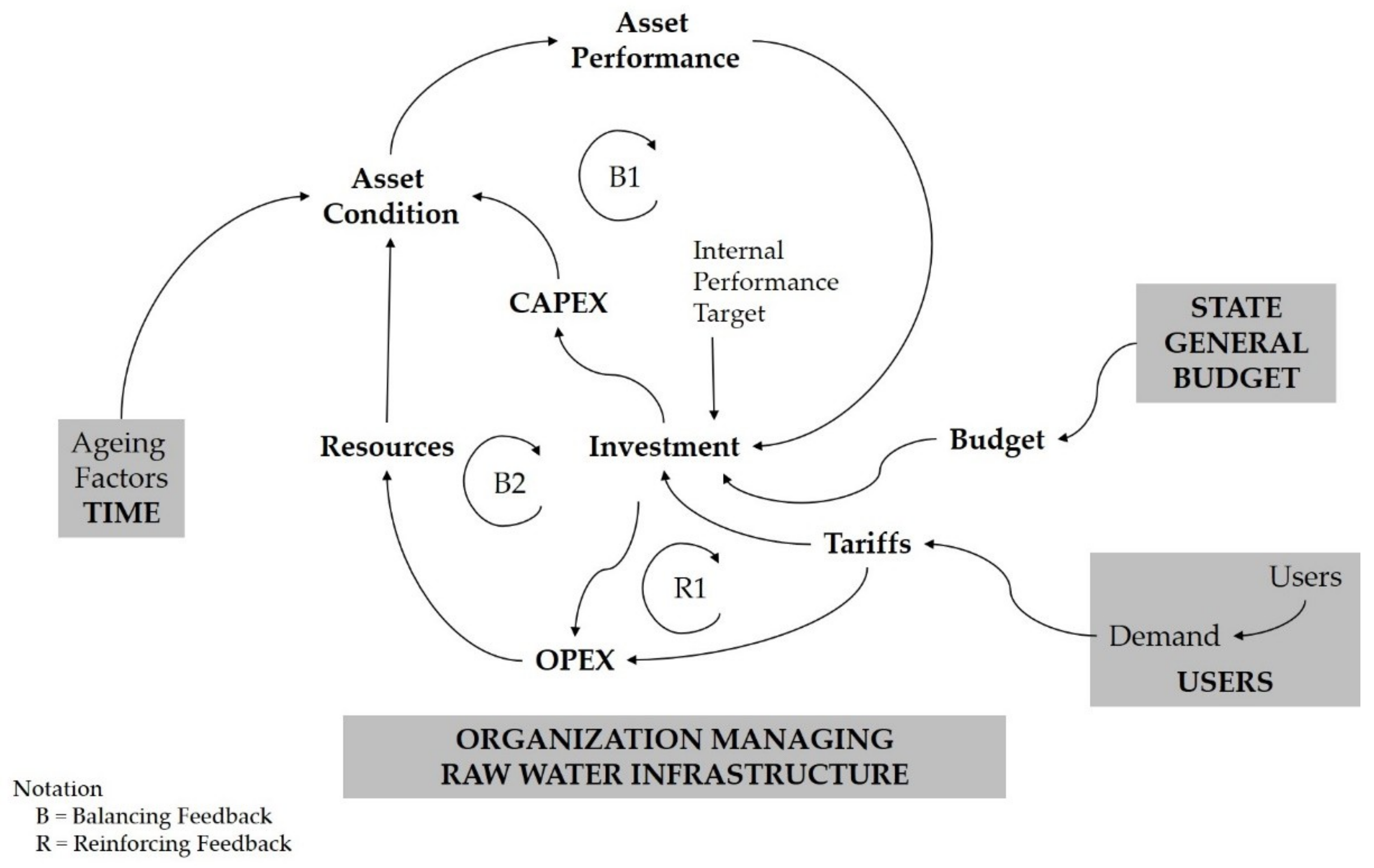
To illustrate the relationships between the different elements of the infrastructure system, a causal loop diagram adapted from Schneider et al. [6] is shown in Figure 1. The sources for investment may come from the State’s general budgets but also from the users, embedded as a part of the water tariffs.
A gap between the actual and the needed expenditure in water management infrastructures has been identified and widely recognized [7,8,9,10,11,12] despite the fact that they are considered as critical infrastructures, that have to be managed through their whole technical life-cycle, assuring a desired level of service and risk [13,14,15,16,17,18]. The literature review shows that there is an extensive development on asset management for water distribution networks [19,20,21,22] but less for primary, raw water infrastructure, including dams and large water conveyance infrastructures [23].
Two key inputs are needed for effective asset management: the asset inventory and the assessment of asset condition.
The asset inventory is the baseline to develop any life-cycle approach to determine the optimal timing for investment [24,25]. One of the problems encountered to apply asset management methodologies is the lack of sound databases [26] and the lack of standardized formats [27,28].
The second key input is the asset condition assessment, as the likelihood of failures related to service and safety levels increases if condition is not adequately identified [29,30,31]. The problem of deterioration in water distribution networks has been studied by different authors, concluding that extensive parts of existing distribution systems need repair and that those systems needing repair are performing below the acceptable standard [32,33,34,35,36].
The assessment of asset condition can be addressed using different approaches. The first approach is the on-line continuous monitoring of condition-related indices of the components of the asset [37]. The main disadvantage of applying this approach is the lack of information available in practice. Another approach is the off-line regular measurements that provide direct or indirect information about condition [38,39]. These techniques are costly and are usually applied when there is a sign of failure. Another possibility is the indirect approach, using operational parameters that are measured in combination with a set of physical and environmental factors to derive condition indices to get insight on the level of deterioration [40]. An alternative approach is to assess condition based on the statistical data of failures and incidents [19,41,42]. Yet, where failures are rare, as it is the case of dams and canals, this method is difficult to apply.
A simplified indirect approach based on asset age and current asset value assessment can be adopted. Many methods of valuing assets are available, including the book value, the written down replacement cost and the market value [43]. A value-based asset condition index is the Infrastructure Value Index (IVI) [44]. Another simplified indirect approach is based on investments on maintenance, repair and rehabilitation, which are compared with the theoretical investments that should have been spent to keep the asset in optimal condition. This comparison is spread through the full life cycle of the infrastructure. This is the concept behind the Asset Sustainability Index (ASI) [45]. The main advantage of these simplified approaches is that they are not asset-specific, and therefore can be applied to a wide variety of typologies. They use estimations of asset value to generate estimations of asset condition, therefore, it is important to know the value of hydraulic infrastructures as assets. Examples of applications of these indices and results obtained can be found in [46,47,48].
This paper focuses on the definition of an inventory of water management assets and on the application and comparison of two approaches to assess asset condition: one based on asset value, IVI, and another based on past maintenance investments and maintenance backlog, ASI. Water infrastructures operated by Segura River Basin authority in Spain are used as case study.
It has been found that the hierarchical structure proposed is adequate to arrange existing information, enabling the calculation of condition indices at different levels of the hierarchy. The indices have been used to get estimates of future condition under different scenarios of investment efforts. In general, good agreement between the two indices used has been found in the prognosis, which provides a more robust basis to inform decisions on asset renewal and maintenance planning. A sensitivity analysis has been performed to address uncertainty in the estimation of one critical aspect, which is the theoretical amount needed for maintenance, as this amount should be defined by the owner according to the organization’s experience and current best practices in the industry. It has been found that using the two indices simultaneously is useful in supporting the decision on what maintenance strategy should be followed in the long term. These indices can also be used to make a preliminary appraisal of the impact of different maintenance strategies on water tariffs.
2. Materials and Methods
2.1. Methodology
2.1.1. Asset Inventory Development
To develop the asset inventory and database structure, a thorough investigation was conducted to track how the information on past investments on renewal, rehabilitation and maintenance had been recorded and managed in the organization in recent decades. As a result of this extensive, lengthy field survey, an asset inventory structure has been proposed, that allows to ease the transfer of information from existing software and paper-format databases.
2.1.2. Asset Hierarchy
The asset inventory is based on a hierarchical structure of the River Basin assets, with four different levels, in a top-down decomposition scheme. The higher level on top or first level is the Operational System (OS) followed by a second level called the Operational Sub-Systems (OSS), a third level called the Assets and a fourth level called the Elements.
An OS comprises the hydrological, infrastructure and water demand dimensions over a certain part of the territory. Each OS in turn can be divided into one or more OSSs, each with their own hydrological, infrastructure and water demand dimensions. Each OSS can be managed independently.
At the Asset Level, the following classification of assets is considered: Storage, Diversion and Flood Protection Facilities, Water Wells, Water Conveyance Facilities, Water Distribution Facilities, Wastewater Treatment Plants and the River Basin’s Hydrologic Information System.
Each asset is further decomposed (fourth level) into one or more different elements that may fall into one of 6 possible types: (1) civil works, (2) electromechanical equipment, (3) electrical equipment, (4) instrumentation equipment, (5) building facilities and (6) access roads. The proposed structure is flexible and is ready to be decomposed into lower levels with more detail in the future, if the organization targets the implementation of asset management practices on a more mature approach. The proposed hierarchical structure is shown in Table 1.
The following set of Equations (1)–(3) describes the logic of the four-level structure proposed, where indices: i, j, k, l are the identification indices for first, second, third and fourth level, respectively. A river basin will be divided into a number of i Operational Systems, OSi, each of them divided into j Operational sub-systems, OSSi,j, where each of them is in turn formed by several k assets, Ai,j,k. Each asset is formed by l different elements, Ei,j,k,l.
2.1.3. Asset Inventory Database Structure
For effective use of existing information on past investments on asset renewal, rehabilitation, repair and maintenance in the assessment of asset condition, the following arrangement for the database structure is created. Based on the information needed for the calculation of asset condition indices that is shown in the next sections, the structure summarized in Table 2 is proposed.
2.2. Asset Condition Assessment
2.2.1. Value-Based Condition Assessment of Assets
The first index used is the Infrastructure Value Index, IVI(t), based on the concept of asset value, and proposed by Alegre et al. [44]. IVI(t), at a given time, t, is the ratio between the current value of an infrastructure at time t, ICV(t), and the replacement cost on modern equivalent asset basis at time t, IRC(t), excluding the salvage value, as shown in Equation (4).
ICV(t) for a given year is estimated assuming a linear depreciation model, the theoretical and actual cumulative budgets in maintenance and a certain salvage value. The model assumes a reference year and constant costs [44]. Reductions in the remaining service life with respect to the expected service life will reduce the infrastructure value. ICV(t) can be estimated at any given year, t, by Equation (5):
where SLR(t) is the Service Life Remaining at time t, in years, and SLE is the total Service Life Expected for the infrastructure analyzed, in years. As the information on past investments is available at Level 4 of the asset inventory, i.e., the element level, the value index of any element, IVI_Ei,j,k,l(t), can be obtained with Equation (6):
where SLR_Ei,j,k,l(t) is the Service Life Remaining of element Ei,j,k,l at time t, and SLE_Ei,j,k,l is total Service Life Expected of element Ei,j,k,l. As stated by Alegre et al. [43], IVI can be seen as a weighted average of the residual lives of the infrastructure components, where the weights are the component replacement costs. Therefore, it is possible to derive IVI values at Asset level, IVI_Ai,j,k(t), as shown in Equations (7):
where RC_Ei,j,k,l(t) is the replacement cost of element Ei,j,k,l at time t. Using this recurrent expression, IVI values at the Operational Sub-system at time t, IVI_OSSi,j(t), can be obtained with Equation (8):
where RC_Ai,j,k(t) is the replacement cost of asset Ai,j,k at time t. Similarly, IVI value at the Operational System at time t, IVI_OSi(t), can be obtained with Equation (9):
where RC_OSSi,j(t) is the replacement cost the whole operational sub-system OSSi,j at time t.
The IVI values of mature, well-maintained infrastructures should be in the vicinity of 50% (40–60%). Higher values point towards one of the following situations: (1) young infrastructures; (2) old infrastructures subject to a recent and significant expansion phase; (3) old infrastructures subject to over-investment in rehabilitation. IVI values below 0.4 reflect accumulated lack of capital maintenance [43]. To help in the interpretation of the results obtained in the following sections it is worth noting that, according to this model, a perfectly maintained infrastructure would have a linear IVI decreasing from 1 at commissioning year to a value of 0.4 at the end of the service life.
2.2.2. Maintenance-Based Condition Assessment of Assets
The second index used is the Asset Sustainability Index, ASI(t), which is defined as the ratio between the Cumulative Amount Budgeted for infrastructure maintenance and preservation over the whole life-cycle of the infrastructure, evaluated at time t, CAB(t), and the total Amount Needed to achieve a specific infrastructure condition over the whole life-cycle of the infrastructure, AN, as shown in Equation (10). The amounts shall include all maintenance actions that contribute to retain the asset in, or to restore the asset to, a certain state, which is the target [44].
For a given time, t, the cumulative amount budgeted, CAB(t), is the sum of two terms. The first term is the sum of past investments accomplished between the time of commissioning of the infrastructure and the year of evaluation, t. The second is the sum of future expected or planned investments between time t + 1 and end of service life year, N. The backlog in investment is defined as the difference between the amount needed and the amount budgeted, and it is reflected in the calculation of CAB(t). As the information on investments is available at Level 4 of the asset inventory, i.e., the element level, the asset sustainability index of any element, ASI_Ei,j,k,l(t), can be obtained with Equation (11):
where CAB_Ei,j,k,l(t) is the Cumulative Amount Budgeted for element Ei,j,k,l evaluated at time t, and AN_Ei,j,k,l is total Cumulative Amount Needed during the service life for element Ei,j,k,l. Similarly, for a certain Asset, Ai,j,k, the asset sustainability index can be calculated with Equation (12):
Taking into account that the cumulative amount budgeted for a certain asset is the sum of the cumulative amounts budgeted for its component elements and that the amount needed is the sum of the amounts needed for its component elements, Equations (13) and (14) can be written.
Combining Equations (11) to (14), the following relationship holds:
The sustainability index at the asset level defined by Equation (15) can be understood as a weighted average of the sustainability indices of its components, where the weights are the total amounts needed for the components. Similar expressions are derived for calculation of the sustainability index at the Operational Sub-system and Operational System levels, as shown by Equations (16) and (17)
A qualitative correlation between ASI and asset condition is defined in Table 3 [45]. To help in the interpretation of the results obtained in the following sections it is worth noting that, according to this model, a perfectly maintained infrastructure without any backlog would have a linear, constant ASI value of 1 throughout the service life.
2.3. Investigation of Case Study
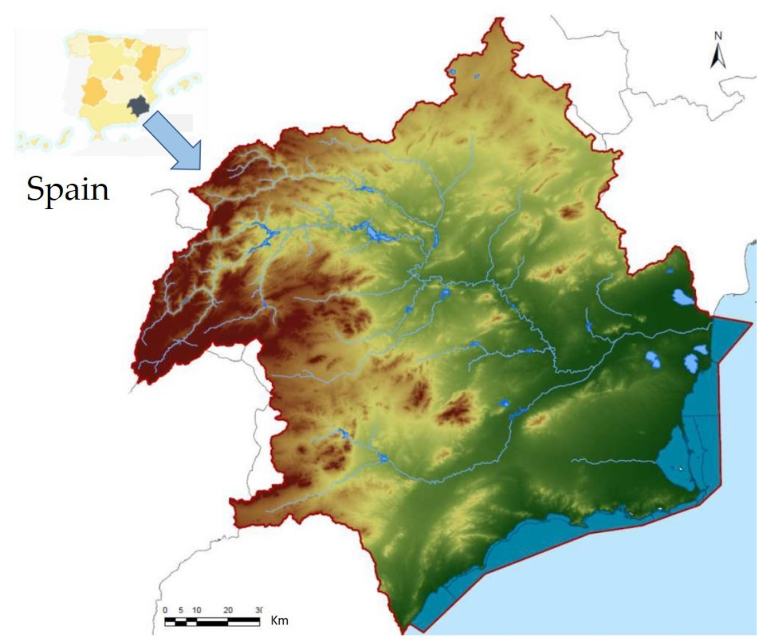
Part of the infrastructures owned and operated by the Segura River Basin Authority in Spain have been used as a case study. The Segura River basin is located on the south-east part of Spain, as shown in Figure 2, with an extension of 20,234 km2.
The average annual rainfall is 385 mm, very unevenly distributed both in space and time. The western part of the river basin corresponds to mountainous areas with maximum elevation of 2000 m above sea level, where most of the rainfall is concentrated, with annual rainfall of 500–1000 mm. The south-eastern part is mostly formed by alluvial plains, draining into the Mediterranean Sea, with annual rainfall below 300 mm. Climate is mild with annual potential evapotranspiration of 993 mm. Average runoff is the lowest in Spain, with a value of 43 mm/year. The main river is the Segura river, with a length of 260 km and annual mean discharge volume of 700 Mm3. The rest of the drainage network is formed by creeks that are dry most of the year, except after events of heavy rainfall. Population in the Segura River Basin is 2,200,000 people. Total water available, including ground water, desalination, reuse and water transfers from other river basins is 1566 Mm3 per year, while total water demand is 1843 Mm3 per year, resulting in an average deficit of 277 Mm3 per year. Agricultural land area is 7720 km2, of which 3865 km2 is irrigated. The operation of the raw water systems in Spain is organized as follows. River basins are divided into one or more independent Operational Systems (OS). Each OSS includes a variety of infrastructure assets (A), including dams, water wells, channels, pipes, pump stations and wastewater treatment plants. The Segura River Basin includes only one OS, divided into 5 different OSS.
Operation and maintenance actions are proposed at the asset level without using a unified methodology, and criteria vary across different types of assets. To the best knowledge of the authors there is not a unified methodology in place used by technical staff managing these infrastructures to elaborate an asset register, to assess the assets’ condition and to evaluate risks associated to critical assets. Most of the information available of past operation and maintenance actions is related to the assigned budgets for operation and maintenance of the different physical assets on a yearly basis. The result is that it is difficult to plan future actions related to the management of these water infrastructure assets, as there is not a clear overall picture of some key features such as past and current asset performance, current asset condition and current and expected asset risk.
The case study focuses on one Operational Sub-System, namely OSS-1, formed by two assets, Asset 1 and Asset 2, selected by the Segura River Authority for this research, which are described in Table 4. The methodology is capable to reach the OS level provided that all OSSs are analyzed.
Expected service life for each asset element and the % of construction costs used to estimate the salvage value are shown in Table 5, according to current standards inside the River Basin Authority [49].
The assessment of the amount needed is a key aspect for successful use of the index. Estimating the amount needed should take into account the past experiences of the organization together with industry best practices. The amount needed per year is estimated as a fraction of the initial value of the asset, using a parameter, m. The maintenance budget percentages associated with parameter ‘m’ should be understood as an estimate of the minimum maintenance budget which should be provided every year in relation to current replacement costs of the infrastructure, in order to provide a basis for ongoing service delivery. The following aspects are embedded in the average annual costs: normal maintenance, emergency maintenance and periodic refurbishment. Based on a detailed review of more than 40 years of maintenance practices inside the organization and international best practices [49,50], the maintenance budget percentages used to test the methodology are shown in Table 6. Records of maintenance investments are included in the Supplementary Materials.
3. Results
The presentation of results follows a bottom-up logic, starting at the element level, and then integrating the results at asset and operational sub-system levels.
3.1. Results of Element Condition (Level 4)
3.1.1. Results for Elements of Asset 1
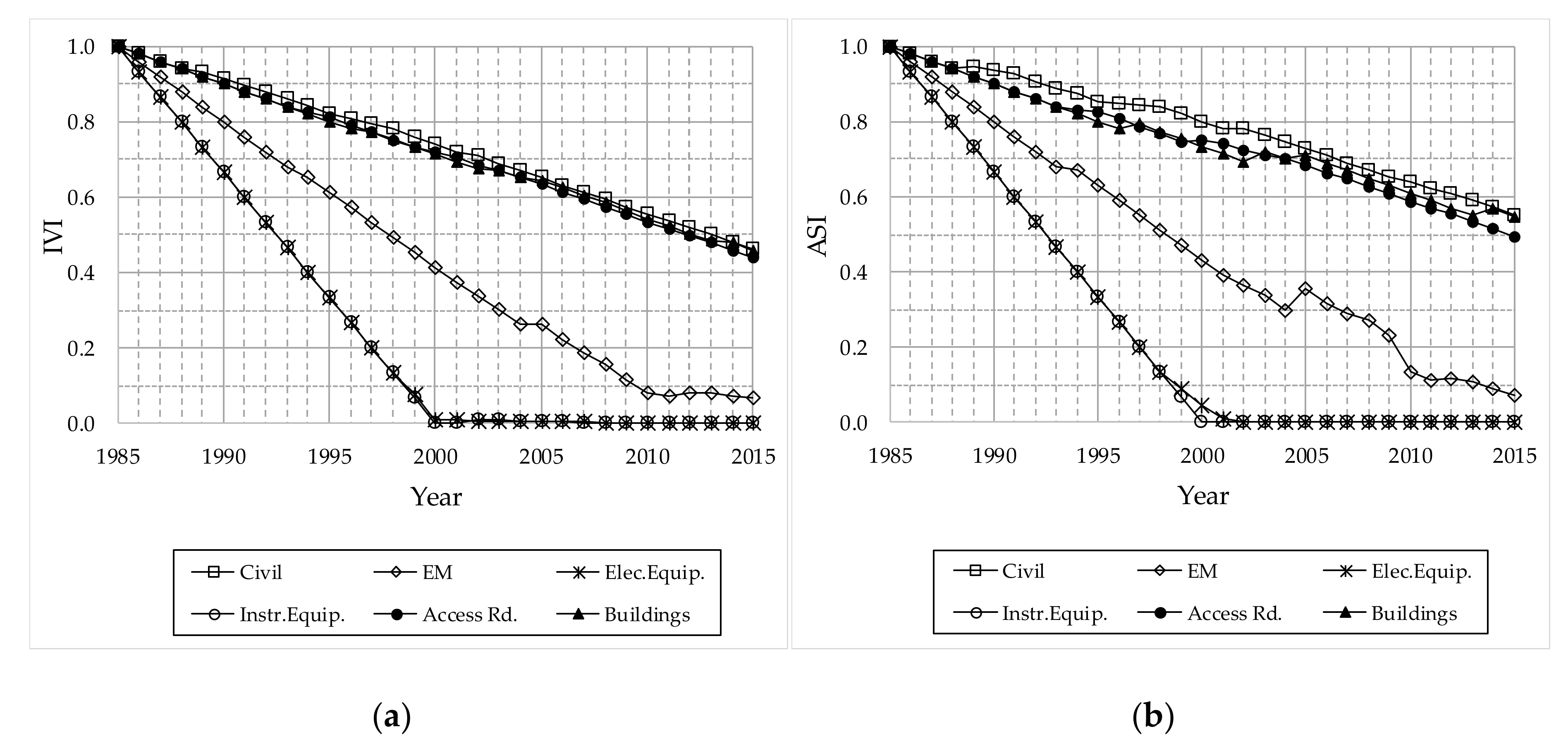
Asset 1, which is a Storage Facility, is formed by a gravity dam, height 61 m, and reservoir volume 246 Mm3. Table 1 shows the breakdown of total cost between the different elements: civil works (92.8%), electromechanical equipment (2.6%), electrical equipment (0.9%), instrumentation equipment (1.7%), building facilities (0.5%) and access roads (1.5%). Figure 3a,b show the results of element condition assessment using IVI and ASI indices, respectively. The period time of analysis is 31 years, from 1985 to 2015. The results according to IVI show that civil elements of the dam, building facilities and access roads are reaching the 0.4 value index after nearly 30 years in service, while with sound maintenance this should have happened at the end of their service life, by year 2035. The electromechanical equipment is lacking maintenance, as it reached the 0.4 value index after 15 years of service, 10 years before its intended service life. Electrical and instrumentation equipment seem to have lacked maintenance since the commissioning of the dam. These results are supported by ASI index calculations. Civil elements of dam, buildings and access roads are entering the medium-poor condition after 30 years of service. Electromechanical equipment has been in very poor condition since the year 2001 (0.4 ≤ ASI < 0.2). According to the results obtained, most of the electrical and instrumentation equipment entered in unpredictable reliability condition at year 1997. Service life of electrical and instrumentation equipment of the dam is 15 years, and the results show not only a lack of maintenance but also that no renewal or replacement of these elements has been provided. The overall picture shows good agreement between IVI and ASI.
3.1.2. Results for Elements of Asset 2
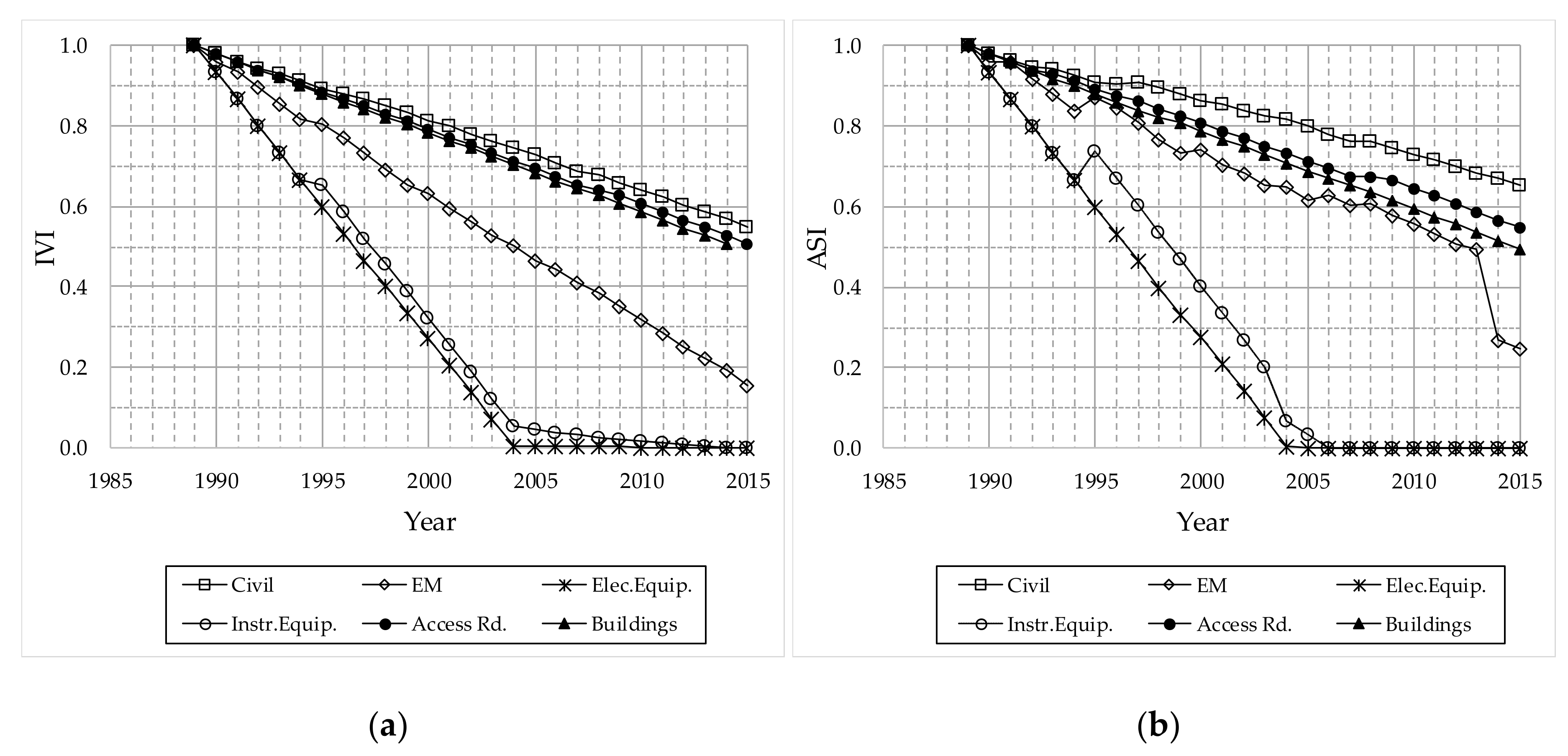
Asset 2 is a water conveyance facility including a channel with maximum capacity of 10 m3/s. Table 1 shows the breakdown of total cost between the different elements: civil works (88.5%), electromechanical equipment (3.1%), electrical equipment (5.3%), instrumentation equipment (0.5%), building facilities (1.7%) and access roads (3.4%). Figure 4a,b show the results of element condition assessment using IVI and ASI indices, respectively. The period time of analysis is 27 years, from 1989 to 2015. The results according to IVI show that civil elements, building facilities and access roads will be reaching the 0.4 value index after nearly 30 years in service, while with sound maintenance this should have happened at the end of their service life, by year 2039. Electromechanical equipment is lacking maintenance, as it reached the 0.4 value index after 18 years of service, seven years before its intended service life. Electrical and instrumentation equipment seem to have lacked maintenance since the commissioning of the dam. Regarding the ASI results, it can be seen that civil elements, buildings and access roads are entering the medium-poor condition after 25 to 30 years of service. Electromechanical equipment has been in very poor condition since the year 2014 (0.4 ≤ ASI < 0.2) due to lack of renewal. Results show that electrical and instrumentation equipment entered in unpredictable reliability condition between the years 2001 and 2002. Results show again not only a lack of maintenance but also no renewal or replacement of these elements. Again, there is good agreement in the diagnosis using both indices.
3.2. Results of Asset Condition (Level 3)
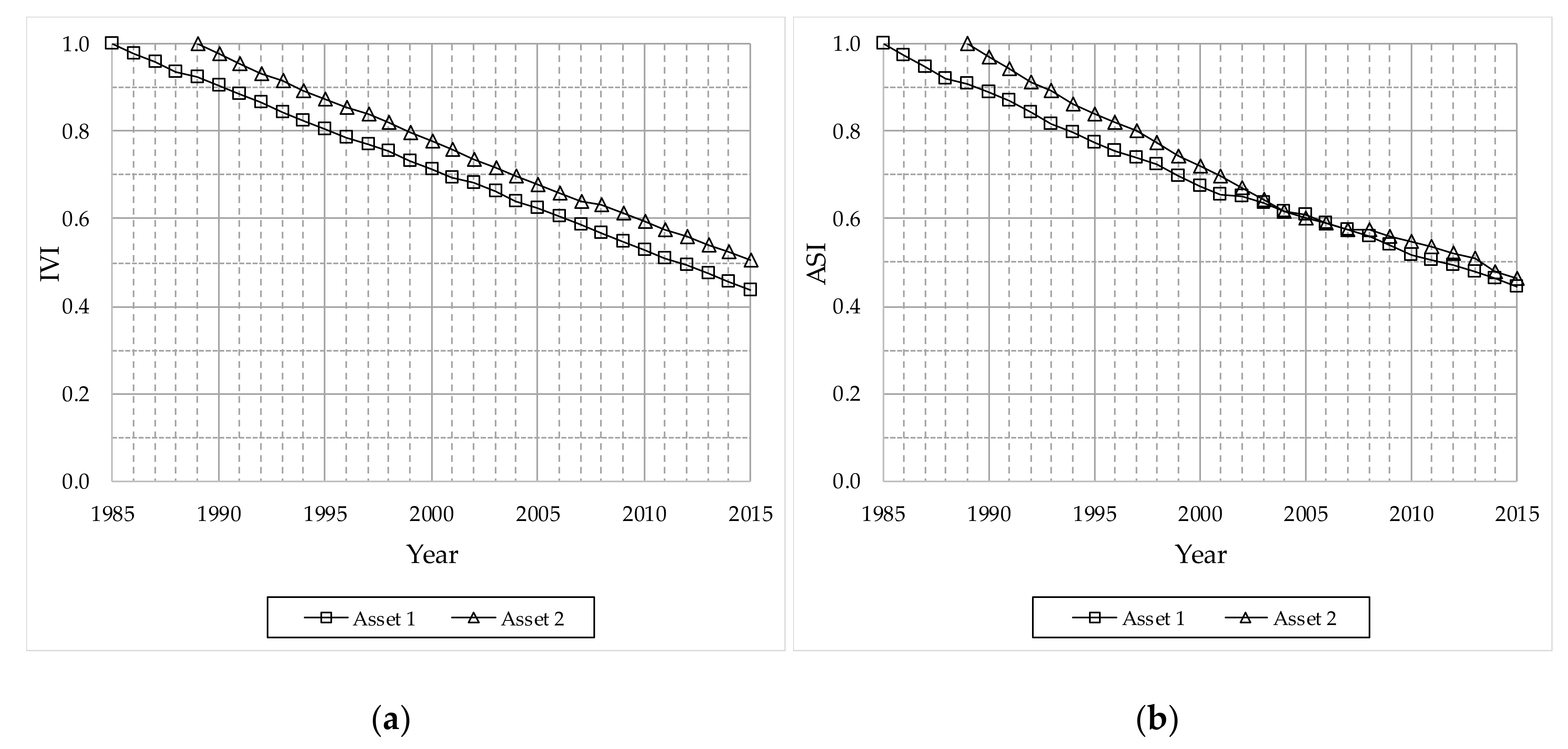
Values of IVI and ASI at the Asset Level can be derived from IVI and ASI values at the Element Level, using Equations (8) and (16), respectively. Figure 5a,b show the results obtained for Asset 1 and Asset 2, respectively. The results with IVI show an overall fair condition for both assets by year 2015, but a lack of maintenance as the target value of 0.4 is going to be reached 15–20 years before the end of the service life. The results with ASI show an overall poor condition for both assets (0.4 ≤ ASI < 0.6) by year 2015, pointing to an accumulated lack of maintenance. The reason for having such values despite the lack of maintenance in some elements such as electrical and instrumentation equipment is found in the weights applied in the calculation of the indices. Both the replacement cost of these elements used in IVI and the amount needed for maintenance used in ASI are much less than for other elements, such as civil works or electromechanical equipment. Therefore, their impact on the overall index value is lower.
3.3. Results of Operational Sub-System Condition (Level 2)
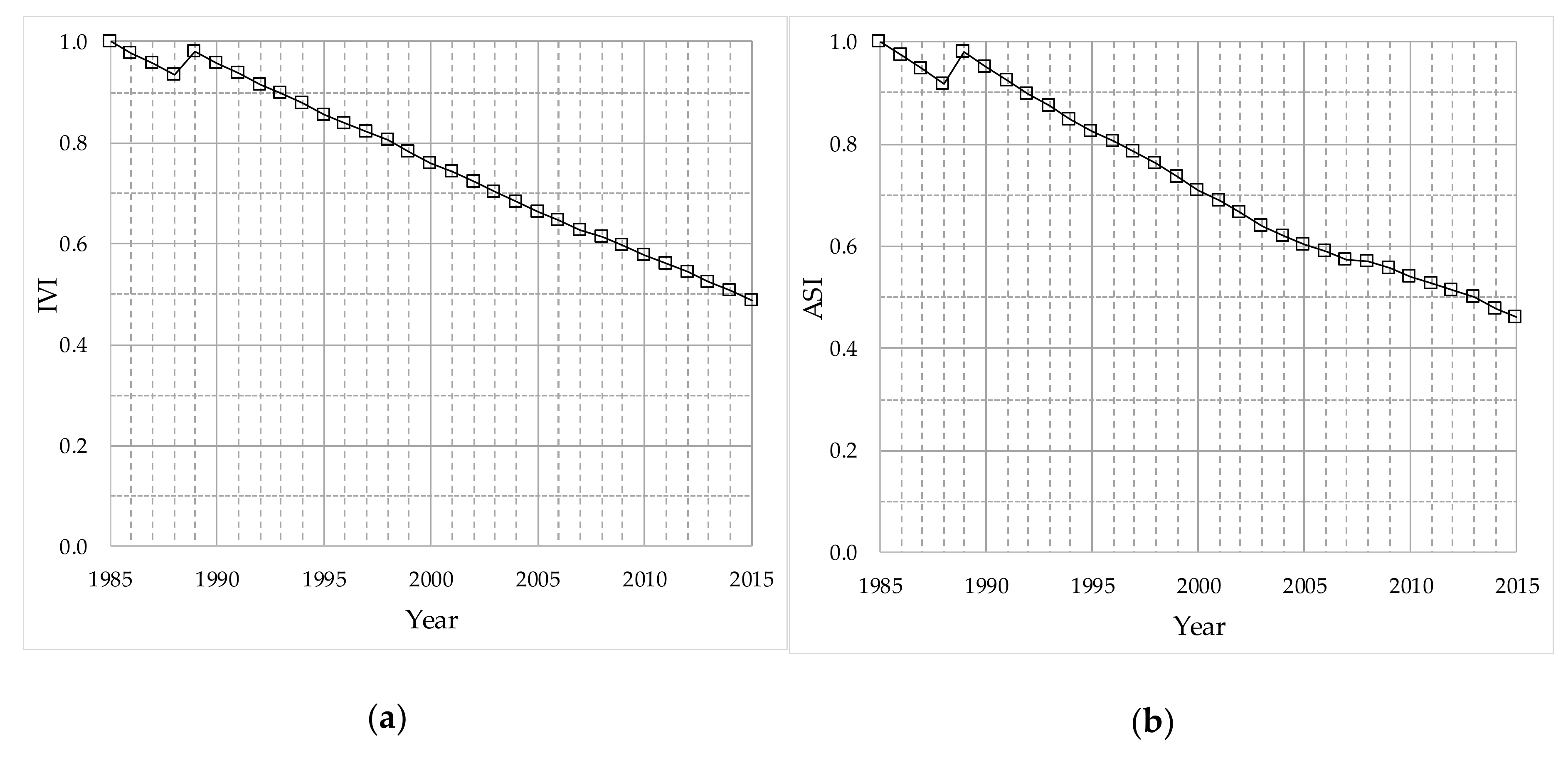
Values of IVI and ASI at the OS-1 Level can be derived from IVI and ASI values at the Asset Level, using Equations (8) and (16), respectively. Figure 6a shows the results obtained using IVI while Figure 6b shows the results with ASI.
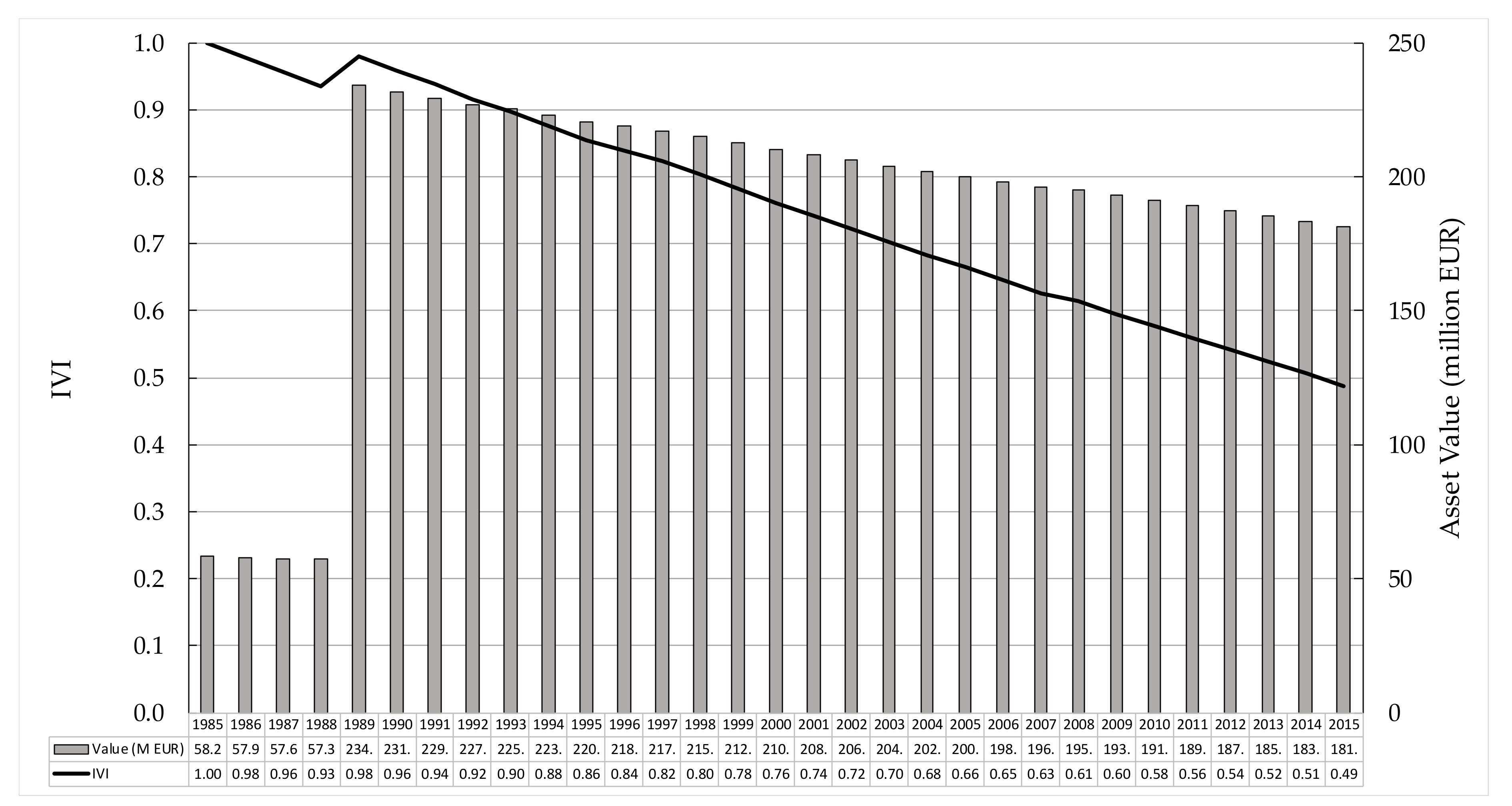
The evolution along time of the total current value of assets of OS-1 and the corresponding IVI values are shown in Figure 7. Current value at a given year is represented by the vertical bars while IVI index is shown as a line. The evolution along time of the backlog in investment and the corresponding ASI values are shown in Figure 8. Cumulative backlog is represented by the vertical bars and the ASI index is represented by the line. The results with IVI show an overall fair condition (0.4 ≤ IVI) whereas the results with ASI show that OS-1 entered the poor condition at year 2006. Accumulated backlog in maintenance investment by year 2015 was approximately 83 million EUR, considered from the commissioning date of assets.
3.4. Sensitivity Analysis
Both indices, IVI and ASI, are influenced by the level of maintenance effort that is considered the adequate or proper, which is estimated through parameter m according to Table 6.
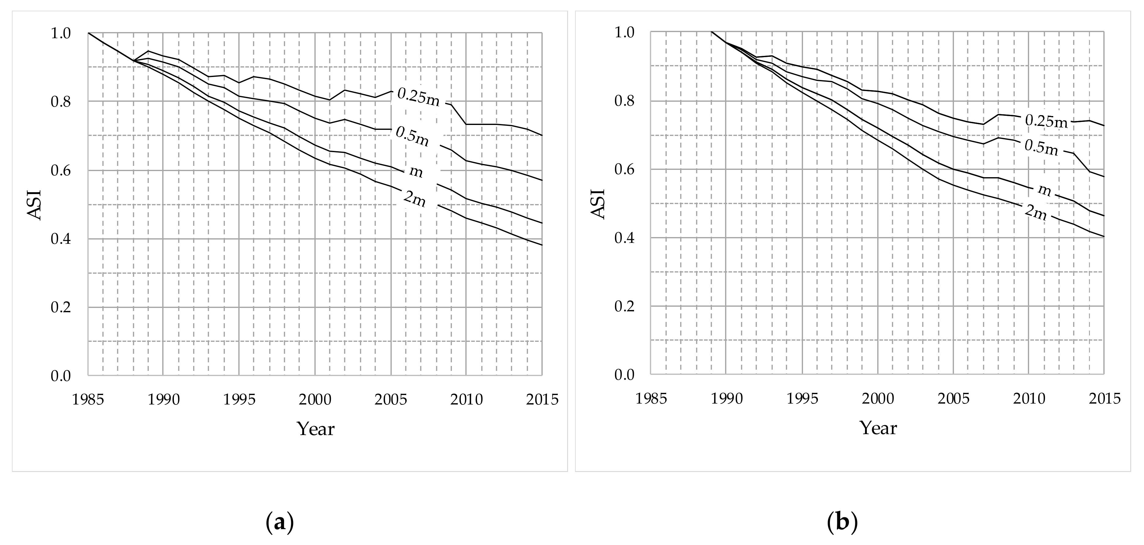
Thus, to explore the effect of m on IVI and ASI indices, the parameter has been scaled by different factors: 0.25, 0.5, 1 and 2, and the corresponding IVI and ASI values have been obtained for Assets 1 and 2, as shown in Figure 9 and Figure 10.
The analysis shows that with lower m values, which means lower amount needed, IVI and ASI values are higher, depicting a better condition of assets, while with higher m values, which means higher amount of investment needed, IVI and ASI values are lower, describing a worse condition of assets. Particularly, if the needed investment effort is set to 25% of that shown in Table 6, the actually performed investment will be considered as adequate, with a minimum backlog. An interesting finding is that doubling the amount needed given by Table 6 does not have a significant influence on IVI and ASI values.
3.5. Assessing Future Asset Condition under Different Scenarios of Investment Effort
3.5.1. Results for Asset 1
ASI and IVI indices can be used to get an approximate picture of future asset condition under different scenarios of future maintenance investment planning. Figure 11 and Figure 12 show the evolution of asset condition with IVI and ASI indices, respectively, together with associated cumulative budget for each scenario.
Several scenarios of investment have been simulated for the period 2016–2034, which corresponds with the service life expected for Asset 1. Each scenario assumes a different investment effort in maintenance for the analysis period. The Base Case is the scenario where planned budget would be equal to the theoretical budget needed according to values of parameter m shown in Table 6 (100%) and the pending renewal of electromechanical, electrical and instrumentation elements is done by year 2016. Three scenarios considering that future investments will be lower and with no renewal of elements are also considered, with efforts corresponding to 75%, 50% and 20% of the theoretical needed, respectively. It should be emphasized that the case with 20% corresponds approximately with the level of investment effort actually performed in the period 1985–2015.
Results with IVI shows that only for the 100% case the asset condition will be over the 0.4 threshold value until year 2022. On the other hand, results with ASI indicates that with the 100% case, the renewal of elements and sustained effort in maintenance improves significantly the index value, masking somehow the ongoing deterioration of civil elements due to previous backlog in maintenance.
3.2.2. Results for Asset 2
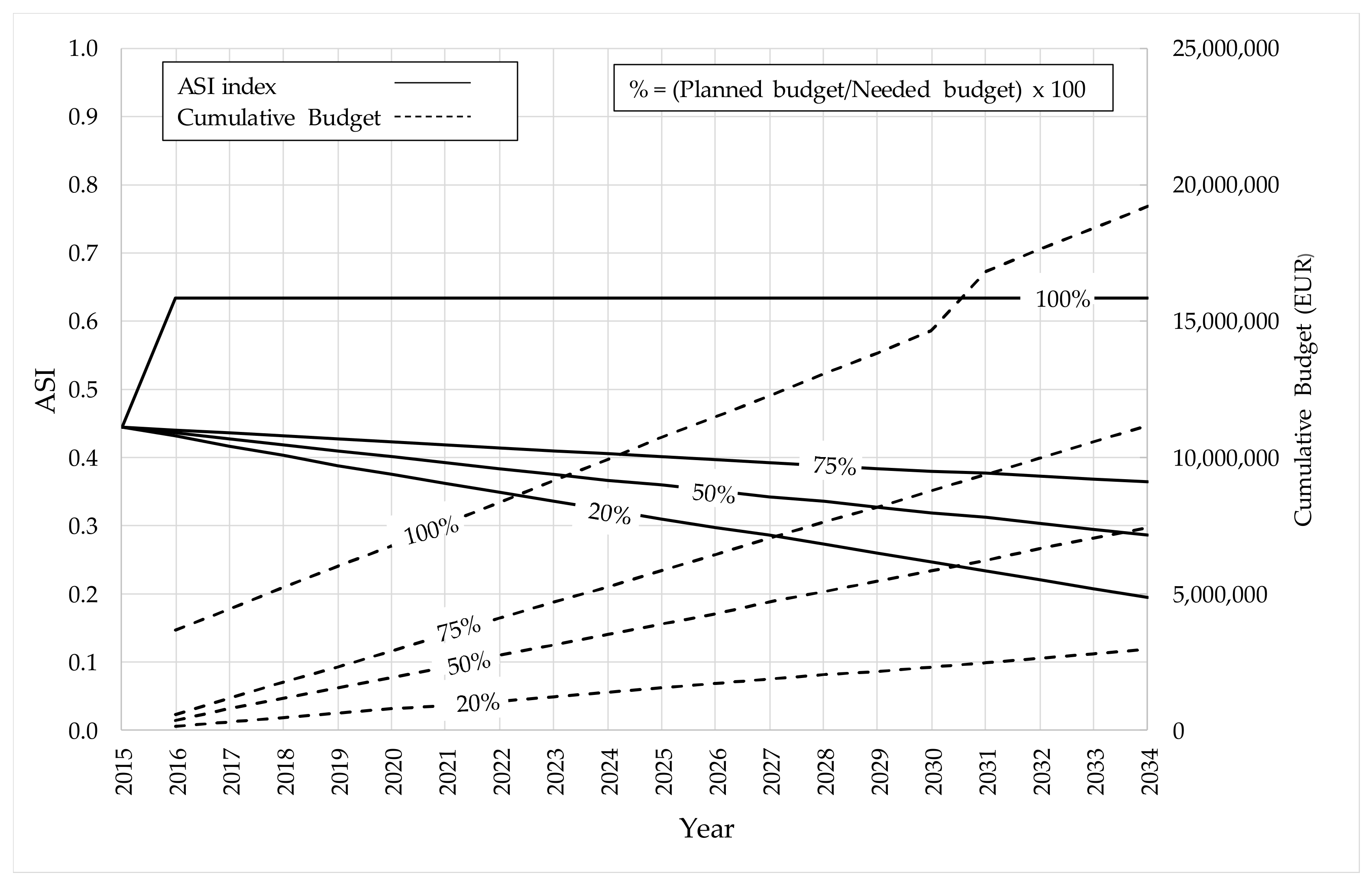
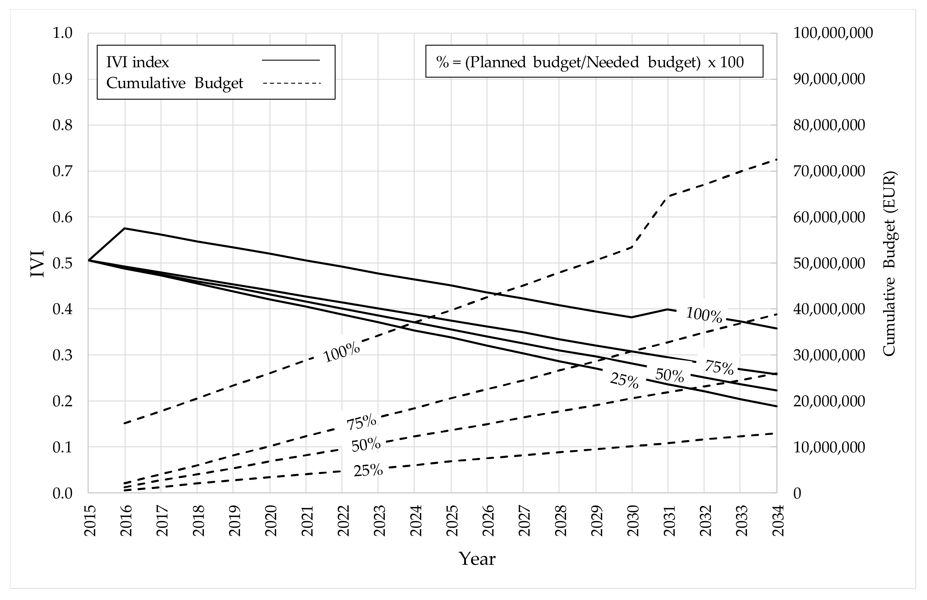
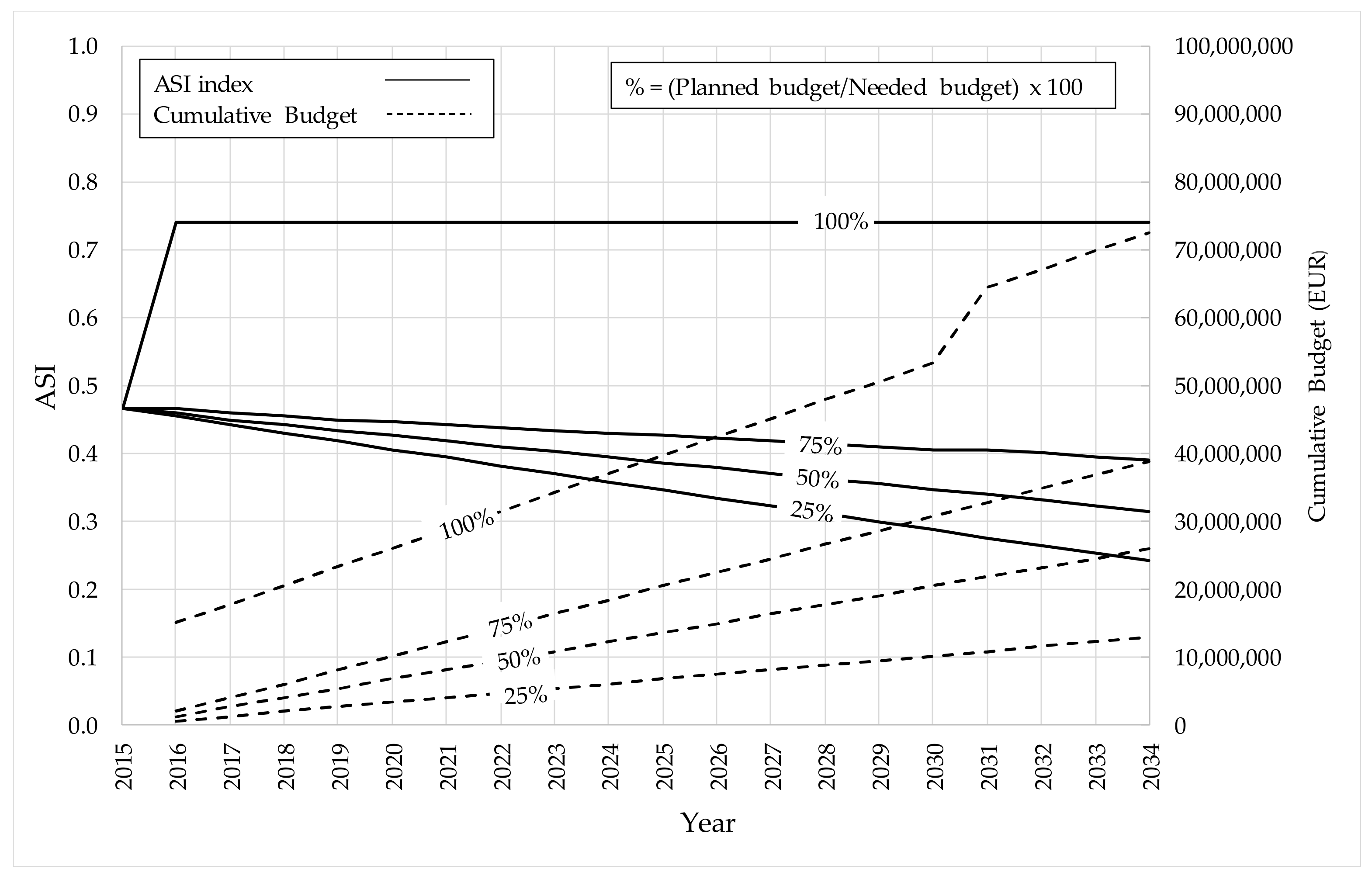
Different scenarios of investment effort have been simulated for the period 2016–2034. Base Case is defined in the same way as Asset 1: maintenance is 100% of theoretical requirement, including pending renewals of elements performed in year 2016. Three scenarios assuming that future investments will be lower than Base Case are considered: 75%, 50% and 25%, where the 25% case corresponds to the real level of investment during the period 1989–2015. Figure 13 and Figure 14 show the evolution of asset condition indices IVI and ASI, respectively, and the associated cumulative budget for each scenario.
Results with IVI show that with the current 25% level of effort, the asset will enter the Below Average Condition (IVI < 0.4) by year 2021, while in the 100% case this will happen in year 2029.
Results with ASI shows that with the current 25% effort the asset will enter in the Very Poor Condition zone by year 2020. ASI index value improves significantly in the 100% case, due to the effect of renewal of elements.
4. Discussion
4.1. Asset Inventory
To analyze asset condition, it was necessary to develop an asset inventory with a proper asset database structure, based on the available information on past investments on asset renewal, asset rehabilitation and asset maintenance. The asset inventory proposed is based on a hierarchical structure of the River Basin Assets, considering a top-down decomposition scheme in four levels: OS, OSS, Assets and Elements, which have been classified into one of six possible categories: civil works, electromechanical equipment, electrical equipment, instrumentation equipment, building facilities and access roads. This structure has been found to be adequate to arrange existing information enabling the calculation of different asset condition indices. In any case, it is needed to have good databases on maintenance investments to apply the proposed methodology.
Though the asset database has been adapted to the features of the Segura River Basin, its structure and the methodology can be applied without limitations to other river basins, as long as the data needed for the calculation of condition indices is available and arranged in the correct format. An advantage of raw water infrastructure systems is that they offer relatively less complexity than water distribution systems, which have many more data challenges.
A storage facility (Dam, Asset 1) and a water conveyance infrastructure (Channel, Asset 2) have been used as target assets.
4.2. Main Parameters in the Calculation of the ASI and IVI Indices
The parameter reflecting the average amount of investment needed per year, m, shown in Table 6 has been estimated based both on national and international published recommendations and practices. As this parameter is relevant in the estimation of IVI and ASI indices, a sensitivity analysis has been performed. It has been found that IVI and ASI numerical values increase significantly when the needed investment is reduced. This feature of the indices makes it necessary to carefully evaluate the values adopted for parameter m before any decision making after asset condition assessment, as different outcomes of current condition are obtained depending on the value selected for the amount needed for maintenance. To explore the range of variation of both indices, a wide range of variation of parameter m has been adopted, including values of 2 × m that are not considered realistic. An interesting result of the analysis performed is that both indices tend to stabilize, with relatively small further reductions, when m values are increased significantly, as shown in Figure 9 and Figure 10.
Valuing involves calculation of depreciation of assets. Though linear depreciation may not be adequate for all water management assets, it is not common to have sufficient and reliable data to justify the use of a specific non-linear depreciation.
Service life is another main parameter. In the context of the case study analyzed, the service life is determined using a technical guideline [49]. Nevertheless, different values for specific assets can be used if evidence exists that the deterioration of the asset has been significantly higher or lower than the theoretical expectation. Judgement from experienced staff managing the assets is a valuable input to assess service life differently from standards or published recommendations.
As with service life, salvage value is determined based on a technical guideline [49] and may well vary depending on owner criteria or current economic regulations.
4.3. Asset and OSS Condition by Year 2015
Starting at the element level, it has been found that both indices adequately capture the significant lack of maintenance of electromechanical, electrical and instrumentation equipment of assets, as shown in Figure 3 and Figure 4, and that both indices depict a fair condition of civil parts, building facilities and access roads of both assets by year 2015.
At the asset level, both indices describe an overall fair condition by year 2015. A critical point for correctly interpreting the results is the understanding of how asset condition indices at the element level are weighted to produce indices at the asset level. The weighting is controlled by the replacement cost of the elements in IVI and by the amount needed for element maintenance in ASI. Therefore, elements with higher replacement costs and with higher maintenance costs are controlling the numerical value of the indices, respectively. The case study analyzed considers assets where the civil elements represent most of these concepts. Therefore, the IVI and ASI values of assets as a whole are controlled by those of their civil elements. This effect may conceal the existence of a large asymmetry in maintenance investments across different elements. It has been found that overall investment in the period from the commissioning of assets until 2015 is approximately 20% of what is theoretically needed for Asset 1 and 25% for Asset 2.
Moving one level up, into the OSS level, both indices show that after 30 years in service the infrastructure is approaching the condition that would be expected by the end of the 50-year service life, due to an under-investment in maintenance. Thus, an under-investment of 75–80% results in a 40% accelerated ageing effect.
4.4. Future Asset Condition Assessment
The indices have been used to estimate future asset condition under different budget scenarios. Results with IVI index show that investment efforts of 100% of the amount theoretically needed, including pending renewals of elements, should be performed to slow down the deterioration of overall asset condition. Sustaining current investment efforts will lead to poor asset condition well before the end of the service life, likely affecting performance and reliability. As the ASI index is weighted by the maintenance effort per year, the long-term deterioration of civil parts has less weight in ASI than in IVI, due to the lower m values used for civil parts compared with other elements. Therefore, the assessment of m values for civil parts plays a key role in the practical application of the methodology and should be validated with an analysis of the condition and performance of the civil parts.
At the OSS level, the mean annual maintenance cost associated with the current investment effort is approximately 0.85 million EUR per year for the whole system. The level of investment associated with the 100% target is 3.5 million EUR per year. Thus, it would be necessary to increase the current effort in asset maintenance by 2.65 million EUR per year.
Assuming that OSS-1 provides 540 Mm3/year of water resources for irrigation, the impact of achieving the 100% target of maintenance for Assets 1 and 2 in the water tariff for irrigation would be about 0.5 cents of EUR per cubic meter of water. It is informative to put this figure in the context of the current price of water for irrigation paid by users in the Segura River Basin, which is in the range of 12 to 33 cents of EUR per cubic meter.
5. Conclusions
The asset inventory proposed, based on a hierarchical structure, has proven to be adequate to arrange the necessary information for calculating different condition indices as IVI and ASI. Nevertheless, it is important that reliable and good quality information on past investments in maintenance is available.
With the proposed arrangement of condition index calculation, it is possible to assess the condition of elements, assets and OSSs. Provided that all OSSs are analyzed, it is possible to get an overall estimation at the OS level.
Using IVI and ASI at the asset level is useful to compare among different assets, but it may convey a distorted vision of the true asset condition if the analysis does not consider explicitly the breakdown of assets into their component elements. Due to the weighting procedure used in the calculation, care must be taken in the interpretation of results, to avoid diluting the true condition of some elements after aggregating their indices into the asset level indices.
Due to the sensitivity of IVI and ASI indices to the amount needed for maintenance, it is advisable to benchmark the asset condition obtained with the model proposed with other condition or performance related measures, to get a more robust assessment. This is especially important for large civil infrastructures due to their high weight in the overall asset condition assessment. This is also of special interest in budget planning for the future.
The methodology has been proved to be useful in the preliminary determination of the impact of future trends in maintenance budgets over water tariffs, though further research is needed to analyze in depth the implications on users.
The proposed approach has proven to be practical, providing a way to gain insight on the condition of asset portfolio and helping to develop an asset investments program based on asset age and asset condition, under a life cycle planning approach.
Extending the methodology to the rest of the OSSs of the Segura River Basin will provide a valuable input for assessing the cost of transferring the asset portfolio to the next generation in a sustainable manner.
Supplementary Materials
The following are available online at https://www.mdpi.com/2073-4441/11/6/1169/s1. Table S1: Maintenance Investments 1985–2015; Figure S1. Main River Basin Infrastructures.
Author Contributions
Conceptualization, M.U.-M. and L.A.-G.; Data curation, M.U.-M. and B.C.-L.; Investigation, M.U.-M. and B.C.-L.; Methodology, M.U.-M. and L.A.-G.; Validation, M.U.-M. and L.A.-G.; Writing—original draft, M.U.-M.; Writing—review & editing, L.A.-G. and J.G.-B.
Funding
This research received no external funding.
Conflicts of Interest
The authors declare no conflict of interest.
References
- McDonald, R.I.; Weber, K.; Padowski, J.; Flörke, M.; Schneider, C.; Green, P.A.; Gleeson, T. Water on an urban planet: Urbanization and the reach of urban water infrastructure. Glob. Environ. Chang. 2014, 27, 96–105. [Google Scholar] [CrossRef] [Green Version]
- Brown, R.R.; Keath, N.; Wong, T.H.F. Urban water management in cities: Historical, current and future regimes. Water Sci. Technol. 2009, 59, 847–855. [Google Scholar] [CrossRef] [PubMed]
- Bakker, K. From State to market?: Water mercantilization in Spain. Environ. Plan. 2002, 34, 767–790. [Google Scholar] [CrossRef]
- González-Gómez, F.; García-Rubio, M.A.; González-Martínez, J. Beyond the public-private controversy in urban water management in Spain. Util. Policy 2014, 31, 1–9. [Google Scholar] [CrossRef]
- Garcia-Rubio, M.A.; Ruiz-Villaverde, A.; González-Gómez, F. Urban water tariffs in Spain: What needs to be done? Water 2015, 7, 1456–1479. [Google Scholar] [CrossRef]
- Schneider, J.; Gaul, A.J.; Neumann, C.; Hogräfer, J.; Wellβow, W.; Schwan, M.; Schnettler, A. Asset management techniques. Electr. Power Energy Syst. 2006, 28, 643–654. [Google Scholar] [CrossRef] [Green Version]
- Andrews, R. Fair value, earnings management and asset impairment: The impact of a change in the regulatory environment. Procedia Econ. Financ. 2012, 2, 16–25. [Google Scholar] [CrossRef]
- Zayed, T.; Mohamed, E. Budget allocation and rehabilitation plans for water systems using simulation approach. Tunn. Undergr. Space Technol. 2013, 36, 34–45. [Google Scholar] [CrossRef]
- Giustolisi, O.; Berardi, L.; Laucelli, D. Supporting decision on energy vs. asset cost optimization in drinking water distribution networks. Procedia Eng. 2014, 70, 734–743. [Google Scholar] [CrossRef]
- Rehan, R.; Knight, M.A.; Unger, A.J.A.; Hass, C.T. Financially sustainable management strategies for urban wastewater collection infrastructure—Development of a system dynamics model. Tunn. Undergr. Space Technol. 2014, 39, 116–129. [Google Scholar] [CrossRef]
- Zhang, W.; Wang, W. Cost modelling in maintenance strategy optimization for infrastructure assets with limited data. Reliab. Eng. Syst. Saf. 2014, 130, 33–41. [Google Scholar] [CrossRef]
- Ward, B. Integrated Asset Management Systems for Water Infrastructure. Ph.D. Thesis, University of Exeter, Exeter, UK, 2015. [Google Scholar]
- Korving, H.; Langeveld, J.G.; Palsma, A.J.; Beenen, A.S. Uniform registration of failures in wastewater systems (SUF-SAS). In Proceedings of the NOVATECH—6th International Conference, Lyon, France, 25–28 June 2007; GRAIE: Villeurbanne, France, 2007; pp. 957–964. [Google Scholar]
- Makaya, E.; Hensel, O. Water distribution system efficiency assessment indicators—Concepts and applications. Int. J. Sci. Res. 2012, 3, 219–228. [Google Scholar]
- Marlow, D.; Moglia, M.; Cook, S.; Beale, D.J. Towards sustainable urban water management: A critical reassessment. Water Res. 2013, 47, 7150–7161. [Google Scholar] [CrossRef]
- Zio, E. Challenges in the vulnerability and risk analysis of critical infrastructures. Reliab. Eng. Syst. Saf. 2016, 52, 137–150. [Google Scholar] [CrossRef]
- Rahim, Y.; Refsdal, I.; Kenett, R.S. The 5C model: A new approach to asset integrity management. Int. J. Press. Vessel. Pip. 2010, 87, 88–93. [Google Scholar] [CrossRef]
- El-Akruti, K.; Dwight, R.; Zhang, T. The strategic role of engineering asset management. Int. J. Prod. Econ. 2013, 146, 227–239. [Google Scholar] [CrossRef]
- Renaud, E.; Le Gat, Y.; Poulton, M. Using a break prediction model for drinking water networks asset management: From research to practice. Water Sci. Technol. Water Supply 2012, 12, 674–682. [Google Scholar] [CrossRef] [Green Version]
- Stern, J.; Mirrless-Black, J. A framework for valuing water in England and Wales. Util. Policy 2012, 23, 13–30. [Google Scholar] [CrossRef]
- Scholten, L.; Scheidegger, A. Strategic rehabilitation planning of piped water networks using multicriteria decision analysis. Water Res. 2014, 49, 124–143. [Google Scholar] [CrossRef]
- Younis, R.; Knight, M.A. Development and implementation of an asset management framework for wastewater collection networks. Tunn. Undergr. Space Technol. 2014, 39, 130–143. [Google Scholar] [CrossRef]
- Heo, C.G.; Bae, S.J. Life-Cycle Cost Analysis of dams maintenance for decision making. Korea Infrastruct. Saf. Technol. Corp. 2009, 33, 52–67. [Google Scholar]
- Du, F.; Woods, G.J.; Kang, D.; Lansey, K.E.; Arnold, R.G. Life cycle analysis for water and wastewater pipe materials. J. Environ. Eng. 2013, 139, 703–711. [Google Scholar] [CrossRef]
- Lee, H.; Shin, H.; Rasheed, U.; Kong, M. Establishment of an inventory for the Life Cycle Cost (LCC) analysis of a water supply system. Water 2017, 9, 592. [Google Scholar]
- Dlamini, D. Improving Water Asset Management When Data Are Sparse. Ph.D. Thesis, Cranfield University, Bedford, UK, 2013. [Google Scholar]
- Morimoto, R. Estimating the benefits of effectively and proactively maintaining infrastructure with the innovative Smart Infrastructure Sensor System. Socio-Econ. Plan. Sci. 2010, 44, 247–257. [Google Scholar] [CrossRef]
- Davis, P.; Sullivan, E.; Marlow, D.; Mamey, D. A selection framework for infrastructure condition monitoring technologies in water and wastewater networks. Expert Syst. Appl. 2013, 40, 1947–1958. [Google Scholar] [CrossRef]
- Hassan, J.; Khan, F. Risk-based asset integrity indicators. J. Loss Prev. Proc. 2012, 25, 544–554. [Google Scholar] [CrossRef] [Green Version]
- Francis, R.A.; Guikema, S.D.; Henneman, L. Bayesian Belief Networks for predicting drinking water distribution system pipe breaks. Reliab. Eng. Syst. Saf. 2014, 130, 1–11. [Google Scholar] [CrossRef]
- Baily, M.J. Inter-Governmental Co-Operation in the North Sea Oil and Gas Industry; Health and Safety Executive: Bootle, UK, 2002; Available online: http://www.npd.no/English/Om+OD/Internasjonalt+samarbeid/NSOAF.htm (accessed on 5 July 2002).
- Too, E.G. Capabilities for Strategic Infrastructure Asset Management. Ph.D. Thesis, Queensland University of Technology, Brisbane, Australia, 2009. [Google Scholar]
- Rehan, R.; Knight, M.A. Application of system dynamics for developing financially self-sustaining management policies for water and wastewater systems. Water Res. 2011, 45, 4737–4750. [Google Scholar] [CrossRef]
- Salman, A. Reliability-Based Management of Water Distribution Networks. Ph.D. Thesis, Concordia University, Montréal, QC, Canada, 2011. [Google Scholar]
- Kabir, G.; Tesfamariam, S. Evaluating risk of water mains failure using a Bayesian belief network model. Eur. J. Oper. Res. 2015, 240, 220–234. [Google Scholar] [CrossRef]
- Bruaset, S.; Saegrov, S.; Ugarelli, R. Performance-based modelling of long-term deterioration to support rehabilitation and investment decisions in drinking water distribution systems. Urban Water J. 2018, 15, 46–52. [Google Scholar] [CrossRef]
- Ye, X.W.; Liu, T.; Zhang, D.F.; Li, J.; Liu, Z.F.; Zhang, L. Applications of Optical Fiber Sensing Technology in Monitoring of Geotechnical Structures. In Environmental Vibrations and Transportation Geodynamics; Bian, X., Chen, Y., Ye, X., Eds.; Springer: Singapore, 2018. [Google Scholar]
- Hao, T.; Rogers, C.D.F.; Metje, N.; Chapman, D.N.; Muggleton, J.M.; Foo, K.Y.; Wang, P.; Pennock, S.R.; Atkins, P.R.; Swingler, S.G.; et al. Condition assessment of the buried utility service infrastructure. Tunn. Undergr. Space Technol. 2012, 28, 331–344. [Google Scholar] [CrossRef]
- Rizzo, P. Water and wastewater pipe non-destructive evaluation and health monitoring: A review. Adv. Civ. Eng. 2010, 2010, 818597. [Google Scholar]
- Tuhovcak, L.; Taus, M.; Mika, P. Indirect condition assessment of water mains. Proc. Eng. 2014, 70, 1669–1678. [Google Scholar] [CrossRef]
- Kleiner, Y.; Nafi, A.; Rajani, B. Planning renewal of water mains while considering deterioration, economies of scale and adjacent infrastructure. In Proceedings of the 2nd International Conference on Water Economics, Statistics and Finance, Alexandroupolis, Greece, 3–5 July 2009. [Google Scholar]
- Alvisi, S.; Franchini, M. Comparative analysis of two probabilistic pipe breakage models applied to a real water distribution system. Civ. Eng. Environ. Syst. 2010, 27, 1–22. [Google Scholar] [CrossRef]
- Falls, L.C.; Haas, R.; Tighe, S. A comparison of asset valuation methods for civil infrastructure. In Proceedings of the 2004 Annual Conference of the Transportation Association of Canada, Quebec City, QC, Canada, 19–22 September 2004. [Google Scholar]
- Alegre, H.; Vitorino, D.; Coelho, S. Infrastructure Value Index: A powerful modelling tool for combined long-term planning of linear and vertical assets. Proc. Eng. 2014, 89, 1428–1436. [Google Scholar] [CrossRef]
- Federal Highway Administration. Financial Planning for Transportation Asset Management. An Overview; Report 1; US Department of Transportation: Washington, DC, USA, 2015. Available online: https://www.fhwa.dot.gov/asset/ (accessed on 5 June 2018).
- Coelho, S.T.; Vitorino, D.; Alegre, H. AWARE-P: A System-Based Software for Urban Water IAM Planning; IWA LESAM: Sydney, Australia, 2013. [Google Scholar]
- Leitão, J.P.; Coelho, S.P.; Alegre, H.; Cardoso, M.A.; Silva, M.S.; Ramalho, P.; Ribeiro, R.; Covas, D.; Vitorino, D.; Almeida, M.C.; et al. The iGPI Collaborative Project: Moving IAM from Science to Industry; IWA LESAM: Sydney, Australia, 2013. [Google Scholar]
- Federal Highway Administration. Asset Management Financial Report Series: The Vermont Experience: A Case Study; Report 6; US Department of Transportation: Washington, DC, USA, 2017. Available online: https://www.fhwa.dot.gov/asset/ (accessed on 15 May 2019).
- García-Cantón, A. Guía Técnica para la Caracterización de Medidas a Incluir en los Planes Hidrológicos y Estudios de Viabilidad, 1st ed.; CEDEX: Madrid, Spain, 2012. [Google Scholar]
- Construction Industry Development Board. Infrastructure Maintenance Budgeting Guideline. Available online: http://www.cidb.org.za/publications/Pages/Infrastructure-Maintenance.aspx/ (accessed on 21 June 2018).
Figure 1.
Causal loop diagram (adapted from Schneider at al. [6]).
Figure 1.
Causal loop diagram (adapted from Schneider at al. [6]).

Figure 2.
Segura River Basin.

Figure 3.
Element condition assessment of Asset 1: (a) Infrastructure Value Index (IVI) index; (b) Asset Sustainability Index (ASI) index.
Figure 3.
Element condition assessment of Asset 1: (a) Infrastructure Value Index (IVI) index; (b) Asset Sustainability Index (ASI) index.

Figure 4.
Element condition assessment of Asset 2: (a) IVI index; (b) ASI index.

Figure 5.
Asset condition assessment for Assets 1 and 2: (a) IVI index; (b) ASI index.

Figure 6.
Condition assessment for Operational Sub-system 1: (a) IVI index; (b) ASI index.

Figure 7.
Operational Sub-system 1. IVI and Asset Value.

Figure 8.
Operational Sub-system 1. ASI and investment backlog.

Figure 9.
Sensitivity analysis of IVI index: (a) Asset 1; (b) Asset 2.

Figure 10.
Sensitivity analysis of ASI index: (a) Asset 1; (b) Asset 2.

Figure 11.
Asset 1 condition assessment with IVI under several future investment scenarios.

Figure 12.
Asset 1 condition assessment with ASI under several future investment scenarios.

Figure 13.
Asset 2 condition assessment with IVI under several future investment scenarios.

Figure 14.
Asset 2 condition assessment with ASI under several future investment scenarios.


Table 1.
Asset Inventory Hierarchy.
| Level 1 | Level 2 | Level 3 | Level 4 |
|---|---|---|---|
| Operational System | Operational Sub-System | Storage, Diversion and Flood Protection Facilities, Water Wells, Water Conveyance Facilities, Water Distribution Facilities, Wastewater Treatment Plants and the River Basin’s Hydrologic Information System | civil works, electromechanical equipment, electrical equipment, instrumentation equipment, building facilities, access roads |
Table 2.
Inventory Database Structure.
| Field | Description |
|---|---|
| System ID | Alpha-numerical code of operational system the asset belongs to |
| Sub-System ID | Alpha-numerical code of operational sub-system the asset belongs to |
| Asset ID | Alpha-numerical code of the asset |
| Asset name | Asset description, linked with asset ID |
| Asset position | Asset coordinates in geographical UTM system |
| Cost | Construction cost (EUR), referred to a certain base year |
| Commissioning | Date used for the calculation of elapsed years of service |
| Service life | Expected years of service |
| Salvage value | Value of the asset at the end of its economic life |
| Intervention ID | Internal code of the investment and its associated information |
| Intervention class | A: Investment in new elements B: Investments in renewal of existing elements C: Investments in maintenance D: Other investments, such as element upgrading |
| Intervention cost | Monetary value of the investment associated with the intervention |
| Intervention date | Date used for the calculation of time elapsed since the intervention |
| Asset value | Monetary value of the asset at a given year, t |
Table 3.
Asset Condition from Asset Sustainability Index [45].
Table 3.
Asset Condition from Asset Sustainability Index [45].
| ASI | Infrastructure Condition | Reliability |
|---|---|---|
| 0.8 ≤ ASI < 1.0 | Good | Reliable |
| 0.6 ≤ ASI < 0.8 | Medium | Reliable |
| 0.4 ≤ ASI < 0.6 | Poor | Degenerated |
| 0.2 ≤ ASI < 0.4 | Very poor | Degenerated |
| 0 ≤ ASI < 0.2 | Failure | Unpredictable |
Table 4.
Description of assets.
| Asset-1 | Asset-2 | |
|---|---|---|
| System ID | OS-1 | OS-1 |
| Sub-System ID | OSS-1 | OSS-1 |
| Sub-System description | Water distribution system for supply and irrigation of 540 Mm3/year | |
| Asset ID | A-1 | A-2 |
| Asset description | Storage Facility (Gravity dam, height 61 m, reservoir volume 246 Mm3) | Water Conveyance Facility (Channel with max. capacity of 10 m3/s) |
| Base year for costs | 2015 | 2015 |
| Construction cost (M EUR 1) | 58.2 | 176.9 |
| Civil cost (M EUR) | 53.9 | 156.5 |
| Electromechanical cost (M EUR) | 1.5 | 5.5 |
| Electrical cost (M EUR) | 0.5 | 9.3 |
| Instrumentation cost (M EUR) | 1.0 | 0.5 |
| Access road cost (M EUR) | 0.9 | 3.4 |
| Building facilities cost (M EUR) | 0.3 | 1.7 |
| Year of commissioning | 1985 | 1989 |
| Service life (years) | 50 | 50 |
| Salvage Value (M EUR) | 44.6 | 84.2 |
1 Notation: M EUR stands for million EUR.
Table 5.
Asset Service Life and Salvage Value [49].
Table 5.
Asset Service Life and Salvage Value [49].
| Elements | Service Life (Years) | Salvage Value (% of Construction Cost) |
|---|---|---|
| civil works | 50 | 80% (Storage, Diversion and Flood Protection Facilities) 75% (System Information Facilities, SAIH) 50% (Water Wells, Water Conveyance Facilities, Water Distribution Facilities and Wastewater Treatment Plants) |
| electromechanical equip. | 25 | 20% |
| electrical equipment | 15 | 10% |
| instrumentation equipment | 15 | 10% |
| building facilities | 50 | 75% |
| access roads | 50 | 75% |
Table 6.
Amount needed per year.
| Level 4—Elements | m | Amount Needed Per Year |
|---|---|---|
| Civil works | 0.01 | m × Asset Value |
| Electromechanical equipment | 0.04 | |
| Electrical equipment | 0.06 | |
| Instrumentation equipment | 0.06 | |
| Building facilities | 0.05 | |
| Access roads | 0.08 |
© 2019 by the authors. Licensee MDPI, Basel, Switzerland. This article is an open access article distributed under the terms and conditions of the Creative Commons Attribution (CC BY) license (http://creativecommons.org/licenses/by/4.0/).
Share and Cite
MDPI and ACS Style
Urrea-Mallebrera, M.; Altarejos-García, L.; García-Bermejo, J.; Collado-López, B. Condition Assessment of Water Infrastructures: Application to Segura River Basin (Spain). Water 2019, 11, 1169. https://doi.org/10.3390/w11061169
AMA Style
Urrea-Mallebrera M, Altarejos-García L, García-Bermejo J, Collado-López B. Condition Assessment of Water Infrastructures: Application to Segura River Basin (Spain). Water. 2019; 11(6):1169. https://doi.org/10.3390/w11061169
Chicago/Turabian StyleUrrea-Mallebrera, Mario, Luis Altarejos-García, Juan García-Bermejo, and Bartolomé Collado-López. 2019. "Condition Assessment of Water Infrastructures: Application to Segura River Basin (Spain)" Water 11, no. 6: 1169. https://doi.org/10.3390/w11061169
Note that from the first issue of 2016, this journal uses article numbers instead of page numbers. See further details here.