Occurrence of Micropollutants in Wastewater and Evaluation of Their Removal Efficiency in Treatment Trains: The Influence of the Adopted Sampling Mode


1
Department of Engineering, University of Ferrara, Via Saragat 1, 44122 Ferrara, Italy
2
Terra & Acqua Tech Tecnopolo, University of Ferrara, Via Borsari 46, 44121 Ferrara, Italy
*
Author to whom correspondence should be addressed.
Water 2019, 11(6), 1152; https://doi.org/10.3390/w11061152
Submission received: 13 May 2019
/
Revised: 23 May 2019
/
Accepted: 31 May 2019
/
Published: 31 May 2019
(This article belongs to the Special Issue Emerging Contaminants in Water: Detection, Treatment, and Regulation)
Abstract
:The monitoring of micropollutants in water compartments, in particular pharmaceuticals and personal care products, has become an issue of increasing concern over the last decade. Their occurrence in surface and groundwater, raw wastewater and treated effluents, along with the removal efficiency achieved by different technologies, have been the subjects of many studies published recently. The concentrations of these contaminants may vary widely over a given time period (day, week, month, or year). In this context, this paper investigates the average concentration and removal efficiency obtained by adopting four different sampling modes: grab sampling, 24-h time proportional, flow proportional and volume proportional composite sampling. This analysis is carried out by considering three ideal micropollutants presenting different concentration curves versus time (day). It compares the percentage deviations between the ideal concentration (and removal efficiencies) and the differently measured concentrations (removal efficiencies) and provides hints as to the best sampling mode to adopt when planning a monitoring campaign depending on the substances under study. It concludes that the flow proportional composite sampling mode is, in general, the approach which leads to the most reliable measurement of concentrations and removal efficiencies even though, in specific cases, the other modes can also be correctly adopted.
1. Introduction
In planning a monitoring campaign, difficulties may arise in defining the sampling strategy, namely the mode and frequency of sample withdrawal in order to collect a number of samples which can be considered representative of the environment, the phenomenon or the process under study. Limiting attention to the water environment (namely raw wastewater, treated effluent, surface water and groundwater), different sampling modes may be utilized: water samples can be instantaneous (grab samples) or composite. In the second case, the resulting composite samples may be time proportional, flow proportional or volume proportional. Moreover, the reference interval for each composite sample could be 24 h or a fraction of the day (12 h, 4 h, or 3 h) [1]. With regard to withdrawal frequency, it is important to plan the sampling in order to pinpoint the (expected or potential) different behaviors in the occurrence of the compounds under study over a period of time [2,3].
In the case of monitoring campaigns tackling compounds occurring at very low concentrations, in the range of ng/L–μg/L—the so-called ‘micropollutants’—it is fundamental to adopt an adequate sampling strategy and also to report it in detail along with the collected results [4,5,6]. Pharmaceuticals and personal care products, flame retardants and parabens are just some of the groups of (micro)pollutants of emerging concern. There has been a sudden increase in studies and publications dealing with the occurrence of these (micro)pollutants in different water environments, and relative removal technologies, from conventional treatments to the most promising technologies and different treatment trains. Most of them are still unregulated compounds (thus their limits in the case of discharge of a treated effluent into a surface water body have not yet been defined), but attention to their potential effects on the environment and human health is increasing and studies are in progress in many parts of the world [7,8,9].
Micropollutants can also be present in industrial wastewater. For instance, a petrochemical wastewater treatment plant may receive raw wastewater from different production wards within the industrial pole, characterized by a wide spectrum of pollutants. Cattaneo et al. [10] report the case of the petrochemical site of Porto Marghera, near Venice in Italy, where the purpose-built wastewater treatment plant must adhere to (strict) authorized limits for the occurrence of macropollutants (among them: suspended solids, biological oxygen demand, total Kjeldahl nitrogen, and nitrates) and ten micropollutants (the so-called “ten forbidden substances”: cyanides, arsenic, cadmium, mercury, lead, organic chloride pesticides, hexachlorobenzene, tributyltin, polychlorinated biphenyls (PCB), dioxins and polycyclic aromatic hydrocarbons (PAH)) in the treated effluent. Sometimes, regulations may also require that the wastewater treatment plant guarantees removal for a selection of (micro)pollutants, in order to demonstrate that it acts as an efficient barrier against them. It is important to underline that in all these situations, a correct sampling mode must be adopted and clearly reported in detail with the results in order to be able to evaluate how representative and reliable the collected measured concentrations are.
Investigations into the occurrence of micropollutants in wastewater have highlighted that many of them may exhibit a substantial variation in concentration over the day (e.g., sulfamethoxazole and ciprofloxacin, [11,12,13]), the week (e.g., fluoruracil, diatrizoate, iomeprol and iohexol [2]), and the month (e.g., cefazolin and carbamazepine, [3]). Others have drawn attention to the temporal variation and distribution of selected pharmaceuticals in surface water bodies (among them [14,15]).
The issue of the influence of the sampling mode adopted in monitoring micropollutants has been addressed by many researchers in the last 10 years. Only in a few studies has this issue has been addressed with great detail (among them [2,4,5,6,16,17]); more often the issue is remarked on but not well discussed [1]. Particularly interesting are the sophisticated studies carried out by Ort and colleagues in [5,6,16,17] regarding the occurrence of pharmaceuticals and diagnostic agents in raw (municipal and hospital) wastewater and treated effluents, as well as in surface water, leading to suggestions for monitoring campaigns of micropollutants on the basis of the number of pulses containing the substance of interest (i.e., the number of toilet flushes at the sampling location) for a catchment area.
The current paper focuses on this issue following another approach: it faces the question by presenting and discussing numerical examples referring to some (representative) micropollutants characterized by different concentrations versus time curves.
In particular, it refers to three substances presenting very different profiles of concentration over the day (a highly variable compound, a randomly variable compound and a compound with low variability), and for each of them it evaluates: (i) the average daily concentration in the case of grab sampling, 24-h time proportional, 24-h volume proportional and 24-h flow proportional composite sampling; and (ii) the daily mass loading based on the estimated average concentrations and the provided flow rate. Finally, it assesses (iii) the removal efficiency for one of the three substances based on the different values of average concentrations found by applying the different sampling modes. This study ends with the evaluation of the (percentage) deviations between the “measured” concentration obtained by adopting a specific sampling mode and the “ideal” average concentration of each representative compound, as well as the (percentage) deviation between the evaluated removal efficiency and the ideal one.
2. Materials and Methods
This study refers to a “theoretical” case study regarding the occurrence of three micropollutants characterized by a different concentration profile versus time (over the day). The simulated substances do not correspond to three specific compounds, but each of them is representative of a group of compounds with a similar concentration trend versus time (see Section 2.1). In this context, the investigations by [11,12,18,19] clearly show the variations in the concentration of micropollutants in municipal raw wastewaters and hospital effluents over a typical day. These experimental values provide us useful insights into the different possible profiles of concentration of micropollutants and allow us to define theoretical ad hoc curves of concentrations versus time for three different representative scenarios.
As to flow rate, the study refers to a small urban settlement, which, according to the technical literature, is characterized by enhanced variations at well-known day hours [20]. A very similar flow pattern was found for the effluent of a medium-large hospital [12,21,22]. In this context, an ad hoc curve of flow rates versus time (during a typical day) was defined on the basis of literature data and evidences [20,21] (see Section 2.2).
It is important to keep in mind that, in the following, attention has to be paid to the variations in concentrations and flow rate over the day and not to the specific (absolute) values reported in the graphs. This means that considerations and results developed in this study can be applied to a small urban settlement as well as a medium to large hospital characterized by similar concentration profiles but different (maximum and minimum) concentration values (often higher in the hospital effluent, [3,21].
2.1. Definition of Representative Compounds
Three key compounds were considered for the study:
- a substance whose concentration in wastewater presents few but evident variations over the day, such as the diagnostic agents gadolinium and iopamidol [18], the cytostatic agent 5-fluoruracil [2] or the diuretic furosemide and the antibiotic sulphamethoxazole [13]. Such a substance is called a ‘high variability substance’, HV_Sub. During the night, its concentration decreases even lower than the corresponding limit of detection (Lod) for some hours;
- a substance whose concentration in wastewater presents a modest variation over the day, and is also detectable during the night, such as the anti-inflammatory ketoprofen [19], the antiseptic triclosan and the anticonvulsant agent phenytoin [13], and the antibiotic trimethoprim [13,23]. This is called the ‘low variability substance’, LV_Sub. It may happen that during the night its concentration decreases to values below its limit of detection, but only for very short periods;
- a substance whose concentration “randomly” varies over the day, such as the antibiotics ciprofloxacin [12] lincomycin [23], the anti-inflammatories diclofenac [13], and 4-tert octylfenol (a degradation product of a surfactant). This substance is called a ‘random variability substance’, RV_Sub. Its profile pattern is not easily predictable.
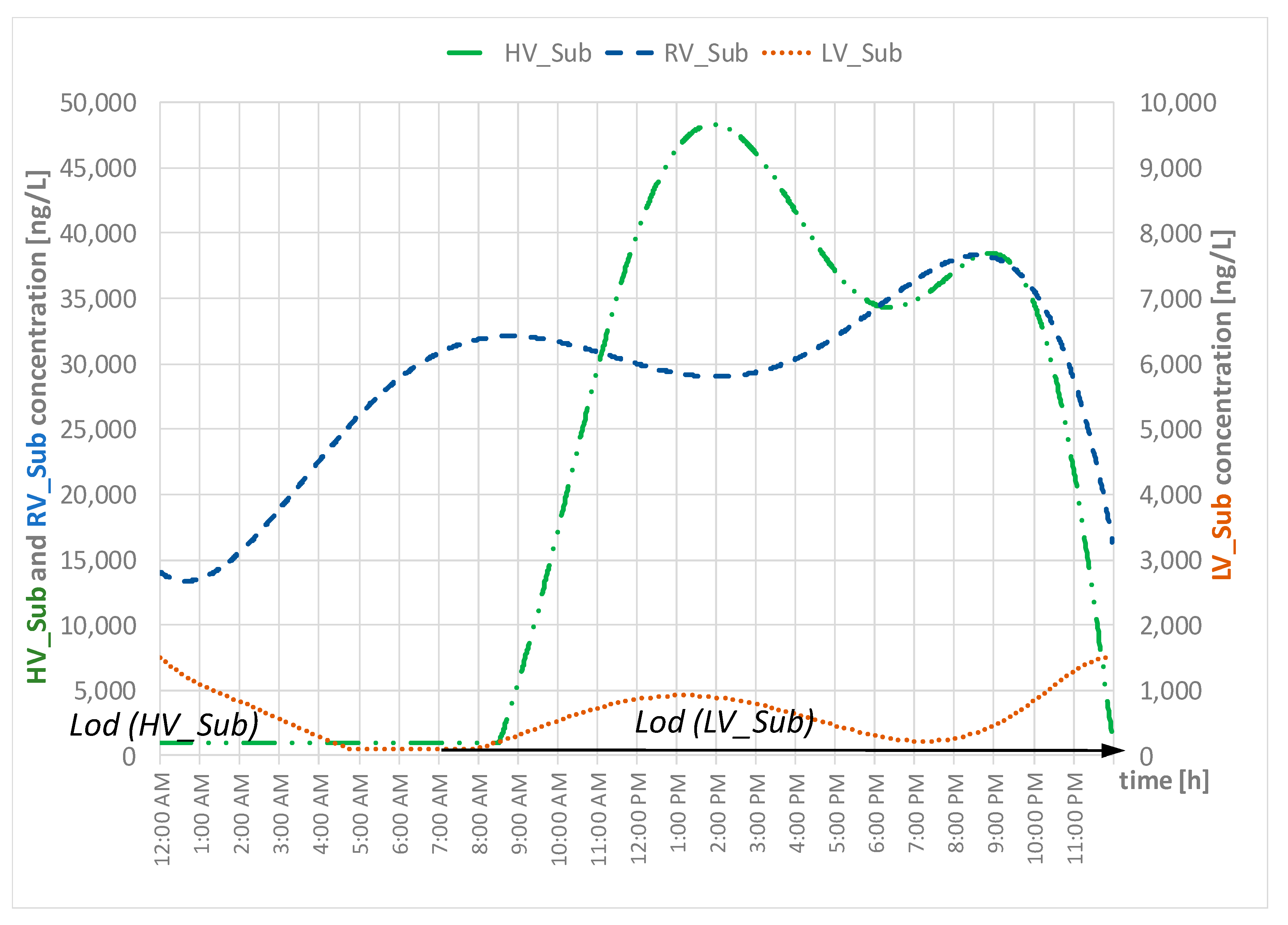
Based on literature data and in particular on the observed temporal variations in concentrations reported for the cited compounds in wastewater [2,4,11,12,13,18,19,23], 24 values of concentrations were set (one for each hour of a day) for the three key compounds (Table S1). Based on them, a nonlinear regression curve was carried out for each substance, by means of the software MATLAB R2018b. The corresponding polynomial functions are reported in Equations (1)–(3) (where concentration is in ng/L and time in min). In this way, the concentration c versus time t curves were set as continuous functions c(t) (Figure 1).
cHV_Sub (t) = 0.015t8 − 0.16t7 + 6.58t6 − 141.33t5 + 1660.2t4 − 10367t3 + 30900t2 − 32689t + 1289.9
cRV_Sub (t) = −0.27t5 + 14.93t4 − 280.73t3 − 1977.7t2 − 2162.1t − 14009
cLV_Sub (t) = +0.008t9 + 0.2t8 − 3.07t7 + 26.93t6 − 126.64t5 + 304.67t4 − 612.86t3 + 1502.8t2
These curves may represent the occurrence in the influent wastewater of a treatment step of three compounds whose characteristics are reported above.
2.2. Flow Rate Curves Versus Time
It was assumed that the flow rate refers to the wastewater generated by a small catchment area (around 3500 inhabitants characterized by an individual water consumption of 200 L/(inhabitant day)) or a medium-large hospital (characterized by around 900 beds with a patient water consumption of 700 L/(patient day), according to literature [21]).
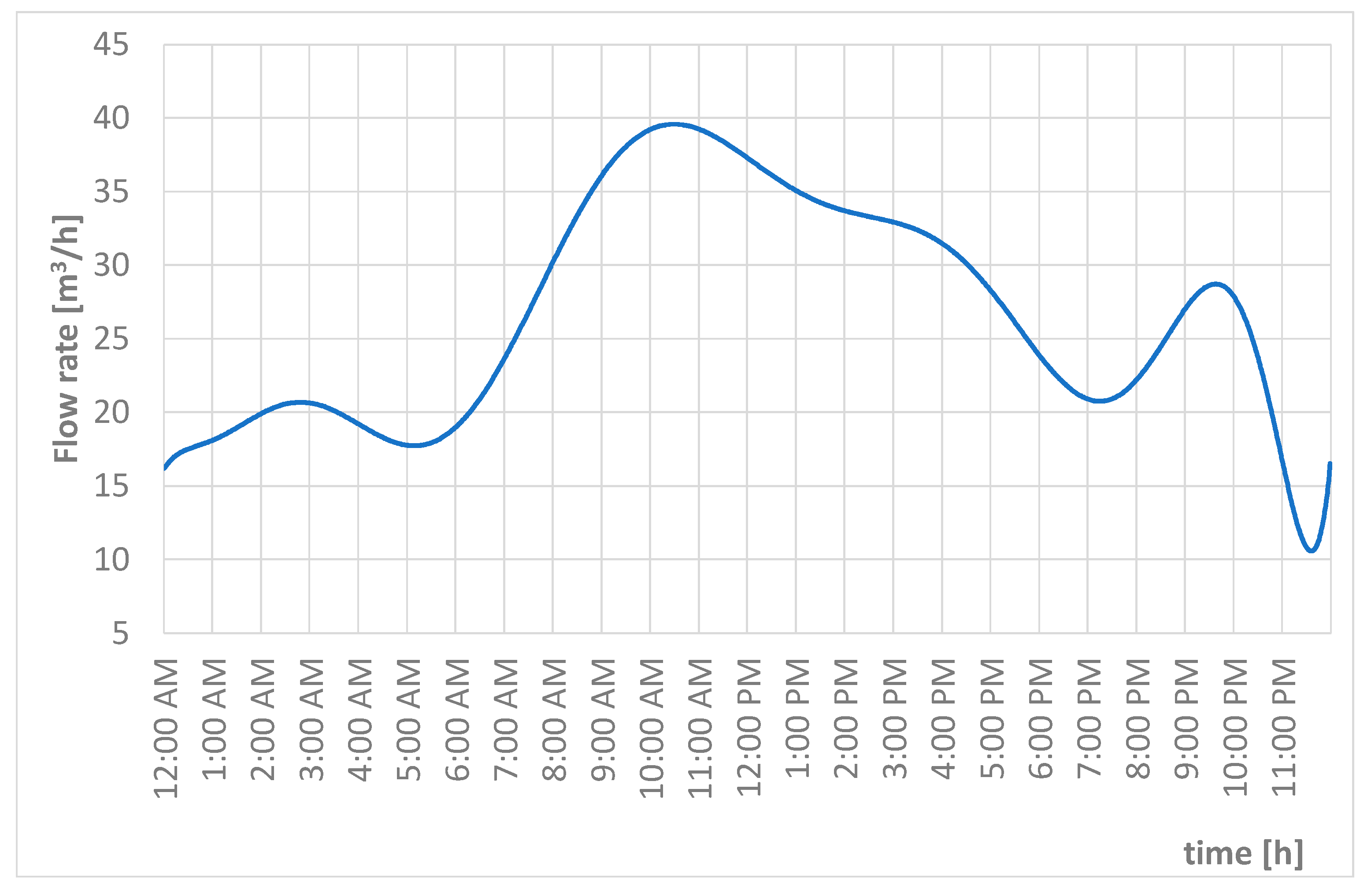
The selection of this size of wastewater source (small urban settlement or medium-large hospital) was in order to obtain more frequent and enhanced variations with regard to a larger urban settlement, as clearly shown by data provided in literature [12,22]. The flow rate referring to the whole day Qdaily is 634.5 m3/d. Based on literature studies on curves of flow rate versus time (day) in settlement/hospital of this size [12,20,22], 24 values of flow rate were set (Table S1) and by software MATLAB R2018b a nonlinear regression was carried out leading to Equation (4) (Q is in m3/h and time t in min). It is reported in Figure 2.
Q(t) = +0.01t11 − 0.11t10 + 0.78t 9 − 3.20t8 + 7.12t7 − 7.77t6 + 5.10t5 + 16.19t4
The wastewater volume flowing as a function of the time V(t) is obtained by the integration of Equation (4):
2.3. The Sampling Modes Adopted and Compared
The sampling modes compared in this study are those defined in Table 1:
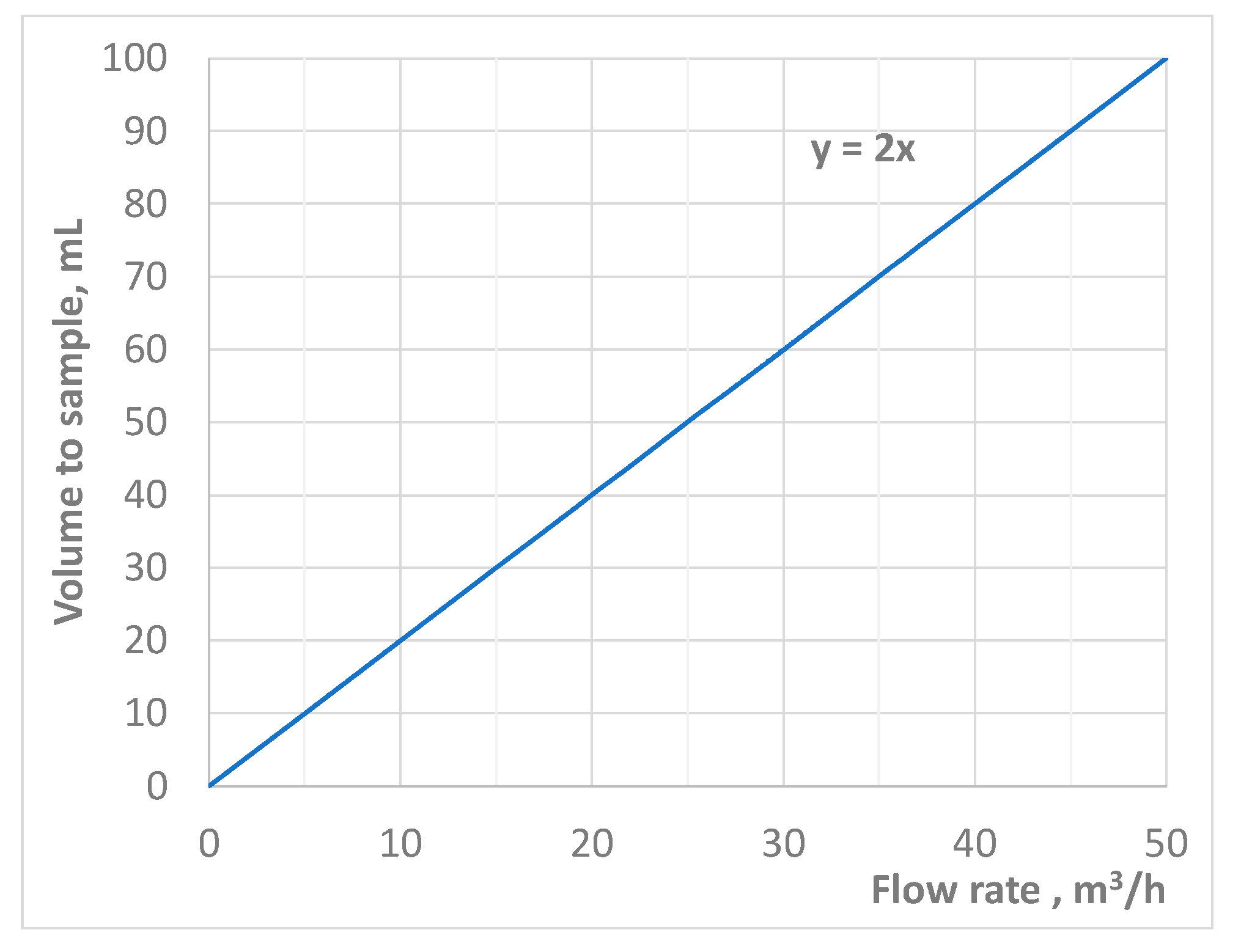
With regard to the flow proportional sampling mode, in order to define the direct proportionality curve between wastewater to be sampled and the flowing wastewater flow rate, the expected range of variability of the flow rate has to be known. In the case study, the observed range varied between 17.3 m3/h and 38 m3/h but, for the sake of caution, it was supposed that it might vary between 10 m3/h and 50 m3/h. It was then supposed that in the case of a flow rate of 10 m3/h, the volume to sample would be equal to 20 mL, and in the case of 50 m3/h, the volume to sample would be 100 mL, resulting in the linear relationship between volume to sample (y) and flow rate (x) y = 2x (Figure 3). Other direct proportional curves could be assumed for different cases.
In order to complete the analysis and the comparison among the available sampling strategies, the Supplementary Material contains Figures S1–S4 showing some details of the different sampling modes. Each graph remarks on the number and volume of samples withdrawn and the instant at which wastewater samples are taken in order to have all the information necessary to obtain the average concentration of the compound under study according to the adopted sampling approach. The flow rate curve versus time is also drawn in order to remark how variations in the flow rate may affect the evaluation of the micropollutant average concentration.
2.4. Daily Average Concentration Evaluation
The ideal (true) obtainable concentration cideal for each compound was evaluated by means of Equation (6):
where ci is the concentration (ng/L) at minute i (in total 60 × 24 min = 1440 min) and Qi is the flow rate (L/min) at the same minute i. Note that Qi is numerically equal to the volume flowing during the minute i (Vi). The concentration value can be considered an accurate value (on a minute measurement basis) of the concentration of the compound. A shorter time interval could also be assumed, for instance the second, and in this case i varies up to 86,400.
The average concentrations of the key compounds were evaluated by assuming the different sampling modes. Note that, with regard to Figure 1, for the substances HV_Sub and LV_Sub, during the night their concentrations decrease below the corresponding Lod (according to the adopted analytical methods, but this issue is beyond the current study). For the sake of caution, it was assumed that the concentration was equal to the Lod (respectively 1000 ng/L and 100 ng/L). In addition, their corresponding limits of quantification (Loq) were assumed equal to 2500 ng/L and 250 ng/L: when their concentration was below the corresponding Loq, it was set equal to 0.5 Loq, according to [24].
In the case of grab sampling, the daily average concentration (ng/L) of a compound in the wastewater is based on the number n of the water grab samples withdrawn (Equation (7)). They were assumed to be 1, 2, 3 or 4 (as described in Table 1):
where ci is the concentration of the key compound in sample i in ng/L.
In the case of 24-h time proportional composite sampling, the daily average concentration of the key substance was evaluated according to Equation (8):
where ci is the concentration (ng/L) of the key compound in sample i, Vsample is the wastewater volume sampled (mL) at each withdrawal (always the same) and k is the number of samples taken according to the defined monitoring protocol (Table 1).
In the case of 24-h flow proportional composite sampling, the daily average concentration of the key substance (ng/L) was evaluated according to Equation (9):
where ci is the concentration of the key compound in sample i, in ng/L, Qi is the withdrawn wastewater volume (mL), being the coefficient of direct proportionality (equal to 2) between the flow rate Qi flowing at the sampling point at that instant and the volume to be sampled (see graph in Figure 2).
In the case of 24-h volume proportional composite sampling, the daily average concentration of the key substance (ng/L) was evaluated according to Equation (10):
where ci is the concentration of the key compound in sample i, in ng/L, and Vsample the wastewater volume (mL) sampled exactly after that the defined fraction of the daily volume of wastewater produced (Vdaily) is flowed. Note that numerically, Vdaily corresponds to Qdaily.
For the sake of clarity, it is here reported the sequence of steps necessary to obtain the average concentrations resulting from applying the different sampling modes described in Table 1. For grab sampling, time proportional and flow proportional composite sampling modes, the steps are:
- 1.
- definition of the sampling times according to Table 1;
- 2.
- calculation of the values of concentrations at each sampling time defined in the last column of Table 1 for the representative compound under study by the corresponding curve (Equations (1)–(3));
- 3.
- evaluation of the average daily concentration by applying the equation corresponding to the selected sampling mode (Equations (7)–(9)).
For the volume proportional composite sampling mode, the steps are:
- 1.
- definition of the frequency of sampling (k samples), according to the last column of Table 1 and the wastewater volume Vvp (=Vdaily/k) which has to flow before collecting a water sample;
- 2.
- evaluation of the k sampling instants tn, by means of the V(t) curve (Equation (5)) posing V(tn) = n Vvp with n = 1, …, k;
- 3.
- calculation of the values of concentrations at each sampling time tn by the corresponding curve (Equations (1)–(3));
- 4.
- evaluation of the average daily concentration by applying Equation (10).
2.5. Mass Load Evaluation
The daily mass load ML (ng/d) of each substance can be evaluated as the product of the average concentration of the compound of interest (ng/L) according to the different sampling modes (Equations (7)–(9)) and the daily flow rate Qdaily (L/d). It is clear that this is directly proportional to the average concentrations through the daily flow rate (=634.5 m3/d).
2.6. Removal Efficiency Evaluation of a Micropollutant: Considerations and Remarks
As discussed in [25], with regard to a generic wastewater treatment step (Figure 4), the percentage efficiency in removing a specific contaminant j is defined on the basis of the mass loading (corresponding to the product: concentration × flow rate) in its influent (stream number 1) and effluents (stream numbers 2 and 3) at a set time interval, in accordance with Equation (12):
As reported in the caption of Figure 4, the step could produce two different effluents (as in a conventional activated sludge system or in a membrane bioreactor: the clarified effluent or the permeate and the excess sludge). Quite often, the equation used for the evaluation of removal efficiency in an activated sludge system does not consider the occurrence of the (micro)pollutant in the excess sludge (this assumes c3,j = 0) and, as reported in [25], this leads to an “apparent” removal efficiency, generally higher than the total removal efficiency.
In this study we have evaluated removal efficiency in the case of a treatment step with only one effluent stream (namely a polishing treatment by constructed wetlands, lagoons, and rapid filtration). Moreover, the time interval assumed for its evaluation is the day, hence the micropollutant concentrations c1 and c2 (referring to the influent and the effluent) considered are the daily average concentrations obtained by following the different sampling modes described in Table 1, Q1 = Q2, and they are numerically equal to Vdaily.
The ideal removal efficiency was evaluated by means of Equation (13):
where c1,i and c2,i are the micropollutant concentrations (ng/L) at minute i in the influent and effluent respectively, Q1,i and Q2,i are the flow rates (L/min) at minute i in the influent and effluent (Q1,i = Q2,i).
Case Study for the Evaluation of Removal Efficiency
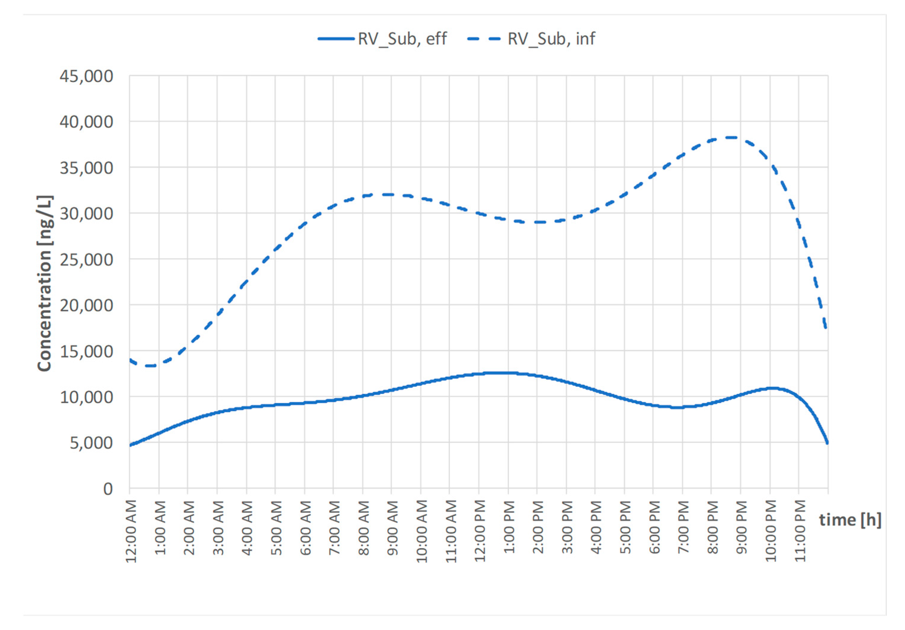
The analysis of the removal efficiency evaluation refers to the data reported in Figure 5, which represents the profile of a randomly variable compound, as described in Section 2.1 for the influent and effluent of a small wastewater treatment plant, characterized by a hydraulic retention time (HRT) of 12 h.
The correlation between the concentration of the key compound and time (min) in the influent corresponds to Equation (2) and for the effluent, to Equation (14). This curve is obtained following the same procedure adopted for Equations (1)–(3) and it is based on the 24 raw data compiled in Table S1:
where t is in minutes and cRV_Sub, eff in ng/L.
cRV_Sub, eff (t) = +0.09t7 − 2.59t6 + 34.09t5 − 206.33t4 − 408.29t3 − 1082.9t2 + 4736.7t1
The removal efficiency for the key compound was evaluated according to the different sampling modes defined in Table 2.
In addition, the removal efficiency of RV_Sub was also estimated, assuming that concentrations were known with a frequency equal to 1 min. This is considered the “ideally obtainable” value of removal efficiency. The collection of this amount of concentrations for many micropollutants is completely unrealistic, due to the high costs and time requested for their analytical determination.
3. Results
3.1. Average Concentration of the Key Compounds
The ideally obtainable daily average concentrations of the three representative compounds were found by applying Equation (6) and are reported in Table 3.
These values are compared here with the average concentrations resulting from applying the different sampling modes described in Table 1, according to the procedure described in Section 2.4. Details of the application of this procedure is reported in Tables S2–S4 with regard only to RV_Sub. For all the substances, the evaluated average concentrations are here reported in tables: Table 4 refers to the case of a different number of grab samples, Table 5 to 24-h time proportional composite sampling, Table 6 to flow proportional composite samples and finally, Table 7 to volume proportional composite samples.
It emerges that for all three substances, average concentrations resulting from the grab sampling mode present the widest ranges of variability, whereas the 24-h flow proportional composite sampling show the smallest ranges of variability. Moreover, one grab sample may lead to an enhanced underestimation or overestimation, depending on the time of sampling and the concentration profile. In the case of a substance with a “flat” curve of concentrations versus time, a grab sample could be considered representative of the “average” daily concentration whatever time it is taken. But in all the other situations, a grab sample should be avoided.
An increment in the frequency of withdrawal for the composite sampling mode always leads to an average concentration measurement, which is closer to the ideal value, whatever the concentration profile.
With regard to the HV_Sub average concentrations reported in Table 4, Table 5, Table 6 and Table 7, it emerges that the lowest value is 1000 ng/L, and the highest is 26,117 ng/L found with the grab sampling mode. This is due to the fact that this substance presents very low concentrations during the night (between 12:00 a.m. and 9:00 a.m. it was below its limit of detection (Lod) and for the sake of caution, was assumed to be equal to its Lod value) and the lowest value corresponds to one grab sample taken at 8:00 a.m. and the highest to four grab samples taken at 8:00 a.m., 12:00 p.m., 4:00 p.m. and 11:00 p.m., with only one sample collected in the interval in which concentrations are very low, assumed equal to the corresponding Lod (1000 ng/L).
With regard to LV_Sub, the lowest average concentration was found with one grab sample (112 ng/L) and the highest with the 24-h volume proportional sample, with samples taken three times a day (818 ng/L).
Finally, referring to RV_Sub, the highest average concentration was found with the grab sample taken at 8:00 a.m. and the lowest average concentration with the 24-h composite sampling mode (three samples taken every eight hours). It is important to observe that the highest value does not correspond to the maximum concentration of the RV_Sub profile of concentration: 38,298 ng/L occurring at 8:35 p.m.
For each of the three substances, the percentage deviation (=) between the ideal average concentration cideal (see Table 3) and the “measured” average concentrations obtained following a specific sampling mode are reported in the three “target” diagrams in Figure 6. The circumferences refer to percentage deviations (1%, 10%, 40% and 100%) on a logarithmic scale. Full symbols represent situations in which the average measured concentration is higher than the corresponding ideal concentration (overestimation) and empty symbols to situations in which the average measured concentration is lower than the corresponding ideal concentration (underestimation).
It emerges that for all three compounds, the sampling mode and frequency which lead to the best estimation of the average concentration are always the 24-h flow proportional composite sampling with samples taken every hour and the 24-h volume proportional composite sampling with 24 samples per day. Moreover, the sampling mode with the smallest deviation is flow proportional: the deviation always remains below 10% with only one exception (HV_Sub with samples taken every eight hours).
It is interesting to observe that the “measured” average concentration is only overestimated (full symbol) for LV_Sub, whereas for HV_Sub and RV_Sub measured average concentrations are underestimated (empty symbols), with just a few exceptions. This fact can be explained by the different concentration profiles versus time of the compounds. Figure 1 shows that LV_Sub is the only compound with night concentrations even higher than diurnal ones and, in the case of time and volume proportional composite samplings (which do not consider the weight of the flow rate) this leads to an overestimation. The ideal average concentration, as shown by the definition in equation 6, weights the concentration with the flow rate, which is lower during the night (Figure 2).
These considerations provide a good explanation as to why time proportional composite sampling could be a good mode for RV_Sub. For this substance, the range of percentage deviations is the smallest in comparison to the range of the other two compounds.
The analysis of the different average concentration values for the three compounds highlights that the selection of the sampling mode which is best suited to the aim of the monitoring campaign depends on the type of substance and on its expected concentration profiles, if known. It could be of interest to know the average concentration of the compound in order to design a treatment train capable of removing it. It could also be of interest to know the highest concentration during the day in case an environmental risk assessment should be carried out (in this case, the European Guidelines [26,27,28] suggest taking the maximum concentration of a compound in order to consider the worst-case scenario). In fact, if the substance has very low concentrations during the night or in well-known daytime intervals, monitoring planning could avoid this period.
3.2. Mass Load Evaluated for Each Substance
The ideal mass loading of each substance was evaluated by Equation (11) and is reported in Table 8. As highlighted in Section 2.5, the percentage deviations with respect to the ideal value of the mass loading of each substance is the same as those found for the average concentrations with regard to the same sampling mode and (obviously) substance.
3.3. Average Removal Efficiency for RV-Sub
The ideally obtainable daily removal efficiency was obtained by applying Equation (13) and is equal to 67.8%. On the basis of the average daily concentrations in the influent and effluent obtained by the different sampling modes (Table 2), the corresponding removal efficiencies were evaluated.
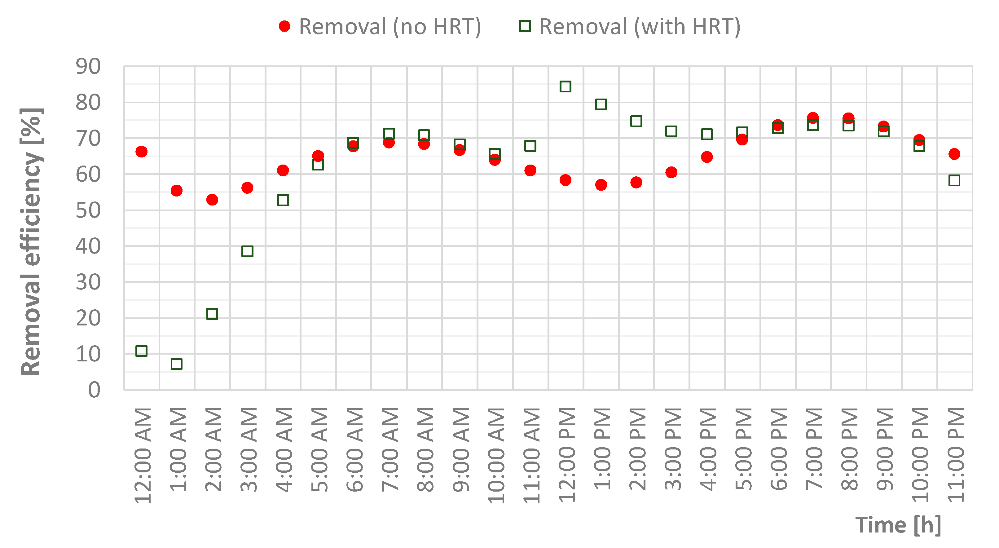
In the first case, a grab sample mode is followed; the flow rate at the entrance and exit of the treatment step is assumed to be the same and samples are taken at the same time (HRT of the treatment step is not considered). The removal efficiency based on only one grab sample during a day and varies between 53% and 76% depending on the sampling time. If samples are taken considering the HRT of the plant (12 h), the removal efficiency varies between 7% and 84%, always depending on the sampling times at the two points. Figure 7 reports the values in both scenarios.
Table 9 reports the RV_Sub removal efficiencies in the case of a different numbers (2, 3, 4) of grab samples taken in the influent and effluent, at the same time (case 1) and considering the HRT of the plant (case 2). It is important to underline that the removal efficiency is evaluated on the basis of the average values in the influent and the effluent of the n grab samples taken as remarked in the last column of Table 2.
It emerges that when HRT is considered, the removal efficiency is always higher than when it is neglected, and it is also higher than the ideally obtainable removal efficiency (equal to 67.8%).
In the case of 24-h time proportional composite sampling, the daily removal efficiency was equal to 65.8%; in the case of 24-h flow proportional composite sampling, the daily removal efficiency was equal to 67.8%, and in the case of 24-h volume proportional composite sampling, the efficiency was 65.4%, all of which are very close to the ideal removal efficiency (67.8%).
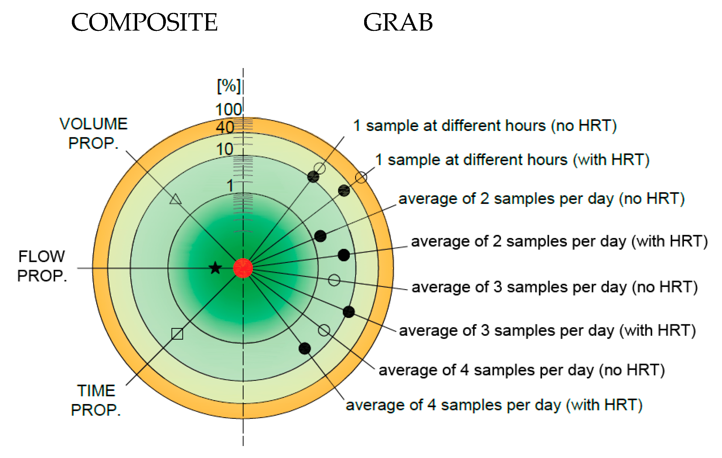
The target graph in Figure 8 reports and compares the percentage deviations (=) between the ideal removal efficiency (67.8%, corresponding to the red circle in the center) and the values found following the different sampling modes.
It emerges that, in the case of removal efficiency based on one grab sample, the ranges of percentage deviations vary between (−22%; +11.5%) without considering HRT and between (−89.6%; +24.2%) if HRT is considered. In case of more grab samples taken in a day, (considering or not considering the HRT), the percentage deviation remains between −5.0% and 11.1%. The flow proportional composite sampling mode leads to the most accurate evaluation (0.06%), compared to time proportional (−2.9%) and volume proportional (−3.5%) modes.
4. Discussion and Final Remarks
This study highlights the influence of the sampling mode on the collected measured concentrations of micropollutants which present different concentration profiles versus time (over the day). It also compares the removal efficiencies achieved in an ideal treatment step when influent and effluent concentrations are collected following different sampling modes. Unfortunately, this is not always reported and described in published papers, as highlighted by [1,5]. In particular in [1], a review dealing with the removal of pharmaceuticals from wastewater by different constructed wetlands, an analysis of the information regarding the adopted sampling modes allows the reader to “weigh up/assess” the reliability of the collected data presented. The most adopted mode in the case of monitoring campaigns regarding micropollutants in different water environments is that of 24-h time proportional composite sampling, whatever the micropollutant and its occurrence profile.
The three “ideal” substances considered in the current study are representative of three different cases and give some insights into the expected scenarios a researcher could find in investigating campaigns in terms of monitoring the occurrence and evaluating the removal of micropollutants. The analysis reported and discussed here provides some figures regarding the expected deviations with regard to ideal values, also called the ‘true’ concentrations and the “true” removal efficiency of a micropollutant. It was found that the flow proportional composite sampling mode leads to the best evaluation of the average concentration of a micropollutant (whatever the concentration profile is) and also of its removal efficiency. It is followed by the volume proportional composite sampling mode, and then by the time proportional one. The grab sample can be adopted if the number of collected samples is able to catch the main (expected) variations of concentrations over the day, in particular when the concentration curve versus time is flat, or when the aim of the monitoring campaign is to find the maximum concentration during the day in case of environmental risk assessment and it is known when it may occur. As most of the micropollutants are unregulated compounds, guidelines for sampling campaigns dealing with them are not available.
To complete the discussion on reliability of collected (measured data) it is important to spend some words on the issue of the uncertainties associated with the direct measurements of concentrations in the water environment. In the current study, it was found that the average evaluated concentrations obtained by applying Equations (1)–(3) and (12) lead to an uncertainty varying in the range between <1% and 30% for 24-h flow proportional composite sampling, between <1% and 40% for 24-h time proportional composite sampling, between <1% and up to 51% for 24-h volume proportional composite sampling and even up to 95% in case of one grab sample in a day.
These values are in agreement with other studies which found uncertainties varying from 10% in the case of 24-h flow proportional composite sampling [17,29] to 25% (even 100%) if time proportional composite sampling is adopted [30]. Regarding uncertainties associated with chemical analysis, literature studies found that they are lower than those for sampling; they may vary between 4% and 16% [31]. Finally, uncertainties in flow rate measurement may vary between 6% according to [17] to 20% according to [32].
These considerations underline the importance of properly defining a sampling mode in order to provide highly reliable data regarding the occurrence and also removal of micropollutants from wastewater.
Supplementary Materials
The following are available online at https://www.mdpi.com/2073-4441/11/6/1152/s1, Table S1: Concentrations of the three representative compounds and values of flow rates used for defining the corresponding profile of concentrations and flow rate over the day (Figure 1, Figure 2 and Figure 5 in the manuscript); Table S2–S4: Evaluation of the average concentrations of the three representative compounds following the different sampling modes; Figure S1: Flow rate profile (dashes) and withdrawn volume (full circles) for each grab sample. Note the volume is always the same at the defined instants of time in case of four grab samples (i.e., 8:00 a.m.; 12:00 p.m.; 5:00 p.m. and 11:00 p.m.); Figure S2: Flow rate profile (dashes) and volume withdrawn (full circles) for the 12 water samples. Also in this case, the sample volume is constant. Samples are taken every 2 h; Figure S3: Flow rate profile (dashes) and volume withdrawn (full circles) for the 12 water samples. The volume taken for the different samples is proportional to the flow rate at the sampling time. Samples are taken every 2 h; Figure S4. Flow rate (dashes) profile and volume withdrawn (full circles) for the 12 water samples. The volume taken for the different samples is constant. Samples are taken when is passed at the sampling point.
Author Contributions
For this research article, both authors contributed extensively to the work. P.V. supervised the research and defined the methodologies; A.G. analyzed the data, P.V: and A.G. contributed to the writing and the review of the paper.
Funding
This research received University of Ferrara funding.
Conflicts of Interest
The authors declare no conflict of interest.
References
- Verlicchi, P.; Zambello, E. How Efficient are Constructed Wetlands in Removing Pharmaceuticals from Untreated and Treated Urban Wastewaters? A Review. Sci. Total Environ. 2014, 470, 1281–1306. [Google Scholar] [CrossRef] [PubMed]
- Weissbrodt, D.; Kovalova, L.; Ort, C.; Pazhepurackel, V.; Moser, R.; Hollender, J.; Siegrist, H.; Mcardell, C.S. Mass flows of X-ray contrast media and Cytostatics in hospital wastewater. Environ. Sci. Technol. 2009, 43, 4810–4817. [Google Scholar] [CrossRef] [PubMed]
- Verlicchi, P. Pharmaceutical Concentrations and Loads in Hospital Effluents: Is a Predictive Model or Direct Measurement the Most Accurate Approach? In Hospital Wastewater—Characteristics, Management, Treatment and Environmental Risks; Springer: Cham, Switzerland, 2018; pp. 101–134. [Google Scholar] [CrossRef]
- Kovalova, L.; Siegrist, H.; Singer, H.; Wittmer, A.; McArdell, C.S. Hospital wastewater treatment by membrane bioreactor: Performance and efficiency for organic micropollutant elimination. Environ. Sci. Technol. 2012, 46, 1536–1545. [Google Scholar] [CrossRef] [PubMed]
- Ort, C.; Lawrence, M.G.; Reungoat, J.; Mueller, J.F. Sampling for PPCPs in wastewater systems: Comparison of different sampling modes and optimization strategies. Environ. Sci. Technol. 2010, 44, 6289–6296. [Google Scholar] [CrossRef] [PubMed]
- Ort, C.; Lawrence, M.G.; Rieckermann, J.; Joss, A. Sampling of pharmaceuticals and personal care products (PPCPs) and illicit drugs in wastewater systems: Are your conclusions valid? A critical review. Environ. Sci. Technol. 2010, 44, 6024–6035. [Google Scholar] [CrossRef] [PubMed]
- Peña-Guzmán, C.; Ulloa-Sánchez, S.; Mora, K.; Helena-Bustos, R.; Lopez-Barrera, E.; Alvarez, J.; Rodriguez-Pinzón, M. Emerging pollutants in the urban water cycle in Latin America: A review of the current literature. J. Environ. Manag. 2019, 237, 408–423. [Google Scholar] [CrossRef] [PubMed]
- Fekadu, S.; Alemayehu, E.; Dewil, R.; Van der Bruggen, B. Pharmaceuticals in freshwater aquatic environments: A comparison of the African and European challenge. Sci. Total Environ. 2019, 654, 324–337. [Google Scholar] [CrossRef]
- Yap, H.C.; Pang, Y.L.; Lim, S.; Abdullah, A.Z.; Ong, H.C.; Wu, C. A comprehensive review on state-of-the-art photo-, sono-, and sonophotocatalytic treatments to degrade emerging contaminants. Int. J. Environ. Sci. Technol. 2019, 16, 601–628. [Google Scholar] [CrossRef]
- Cattaneo, S.; Marciano, F.; Masotti, L.; Vecchiato, G.; Verlicchi, P.; Zaffaroni, C. Improvement in the Removal of Micropollutants at Porto Marghera Industrial Wastewaters Treatment Plant by MBR Technology. Water Sci. Technol. 2008, 58, 1789–1796. [Google Scholar] [CrossRef]
- Paíga, P.; Correia, M.; Fernandes, M.J.; Silva, A.; Carvalho, M.; Vieira, J.; Jorge, S.; Silva, J.G.; Freire, C.; Delerue-Matos, C. Assessment of 83 pharmaceuticals in WWTP influent and effluent samples by UHPLC-MS/MS: Hourly variation. Sci. Total. Environ. 2019, 648, 582–600. [Google Scholar] [CrossRef]
- Duong, H.; Pham, N.; Nguyen, H.; Hoang, T.; Pham, H.; CaPham, V.; Berg, M.; Giger, W.; Alder, A. Occurrence, fate and antibiotic resistance of fluoroquinolone antibacterials in hospital wastewaters in Hanoi, Vietnam. Chemosphere 2008, 72, 968–973. [Google Scholar] [CrossRef] [PubMed]
- Nelson, E.D.; Do, H.; Lewis, R.S.; Carr, S.A. Diurnal variability of pharmaceutical, personal care product, estrogen and alkylphenol concentrations in effluent from a tertiary wastewater treatment facility. Environ. Sci. Technol. 2011, 45, 1228–1234. [Google Scholar] [CrossRef] [PubMed]
- Burns, E.E.; Carter, L.J.; Kolpin, D.W.; Thomas-Oates, J.; Boxall, A.B.A. Temporal and spatial variation in pharmaceutical concentrations in an urban river system. Water Res. 2018, 137, 72–85. [Google Scholar] [CrossRef] [PubMed]
- Barbosa, M.O.; Ribeiro, A.R.; Ratola, N.; Hain, E.; Homem, V.; Pereira, M.F.R.; Blaney, L.; Silva, A.M.T. Spatial and seasonal occurrence of micropollutants in four Portuguese rivers and a case study for fluorescence excitation-emission matrices. Sci. Total Environ. 2018, 644, 1128–1140. [Google Scholar] [CrossRef] [PubMed]
- Ort, C.; Gujer, W. Sampling for representative micropollutant loads in sewer systems. Water Sci. Technol. 2006, 54, 169–176. [Google Scholar] [CrossRef] [PubMed]
- Ort, C.; Lawrence, M.G.; Reungoat, J.; Eaglesham, G.; Carter, S.; Keller, J. Determining the fraction of pharmaceutical residues in wastewater originating from a hospital. Water Res. 2010, 44, 605–615. [Google Scholar] [CrossRef] [PubMed]
- Kummerer, K.; Helmers, E. Hospital effluents as a source of gadolinium in the aquatic environment. Environ. Sci. Technol. 2000, 34, 573–577. [Google Scholar] [CrossRef]
- Khan, S.; Ongerth, J. Occurrence and removal of pharmaceuticals at an Australian sewage treatment plant. Water 2005, 32, 80–85. [Google Scholar]
- Verlicchi, P.; Galletti, A.; Al Aukidy, M. Hospital Wastewaters: Quali-quantitative Characterization and Strategies for Their Treatment and Disposal. In Wastewater Reuse and Management; Springer Science & Business Media: New York, NY, USA, 2013; pp. 225–251. [Google Scholar]
- Verlicchi, P.; Galletti, A.; Petrovic, M.; Barcelo, D. Hospital Effluents as a Source of Emerging Pollutants: An Overview of Micropollutants and Sustainable Treatment Options. J. Hydrol. 2010, 389, 416–428. [Google Scholar] [CrossRef]
- Boillot, C.; Bazin, C.; Tissot-Guerraz, F.; Droguet, J.; Perraud, M.; Cetre, J.C.; Trepo, D.; Perrodin, Y. Daily physicochemical, microbiological and ecotoxicological fluctuations of a hospital effluent according to technical and care activities. Sci. Total Environ. 2008, 403, 113–129. [Google Scholar] [CrossRef]
- Hong, Y.; Sharma, V.K.; Chiang, P-C.; Kim, H. Fast-target analysis and hourly variation of 60 pharmaceuticals in wastewater using UPLC-high resolution mass spectrometry. Arch. Environ. Contam. Toxicol. 2015, 69, 525–534. [Google Scholar] [CrossRef] [PubMed]
- Armbruster, D.A.; Pry, T. Limit of Blank, Limit of Detection and Limit of Quantitation. Clin. Biochem. Rev. 2008, 29, S49. [Google Scholar] [PubMed]
- Verlicchi, P.; Al Aukidy, M.; Zambello, E. Occurrence of Pharmaceutical Compounds in Urban Wastewater: Removal, Mass Load and Environmental Risk After a Secondary Treatment-A Review. Sci. Total Environ. 2012, 429, 123–155. [Google Scholar] [CrossRef] [PubMed]
- European Community (EC). Technical Guidance Document on Risk Assessment in support of Commission Directive 93/67/EEC on Risk Assessment for new notified substances, Commission Regulation (EC) No 1488/94 on Risk Assessment for Existing Substances, and Directive 98/8/EC of the European Parliament and of the Council concerning the placing of biocidal products on the market, Parts I. European Communities, EUR 20418 EN/1. 2003. Available online: https://echa.europa.eu/documents/10162/16960216/tgdpart1_2ed_en.pdf (accessed on 31 May 2019).
- European Community (EC). Technical Guidance Document on Risk Assessment in support of Commission Directive 93/67/EEC on Risk Assessment for new notified substances, Commission Regulation (EC) No 1488/94 on Risk Assessment for Existing Substances, and Directive 98/8/EC of the European Parliament and of the Council concerning the placing of biocidal products on the market, Parts II. European Communities, EUR 20418 EN/1. 2003. Available online: https://echa.europa.eu/documents/10162/16960216/tgdpart2_2ed_en.pdf (accessed on 31 May 2019).
- European Community (EC). Technical Guidance Document on Risk Assessment in support of Commission Directive 93/67/EEC on Risk Assessment for new notified substances, Commission Regulation (EC) No 1488/94 on Risk Assessment for Existing Substances, and Directive 98/8/EC of the European Parliament and of the Council concerning the placing of biocidal products on the market, Parts IV. European Communities, EUR 20418 EN/1. 2003. Available online: https://echa.europa.eu/documents/10162/16960216/tgdpart4_2ed_en.pdf (accessed on 31 May 2019).
- Jelic, A.; Fatone, F.; Di Fabio, S.; Petrovic, M.; Cecchi, F.; Barcelo, D. Tracing pharmaceuticals in a municipal plant for integrated wastewater and organic solid waste treatment. Sci. Total Environ. 2012, 433, 352–361. [Google Scholar] [CrossRef] [PubMed]
- Verlicchi, P.; Zambello, E. Predicted and measured concentrations of pharmaceuticals in hospital effluents. Examination of the strengths and weaknesses of the two approaches through the analysis of a case study. Sci. Total Environ. 2016, 565, 82–94. [Google Scholar] [CrossRef] [PubMed]
- Verlicchi, P.; Al Aukidy, M.; Jelic, A.; Petrović, M.; Barceló, D. Comparison of Measured and Predicted Concentrations of Selected Pharmaceuticals in Wastewater and Surface Water: A Case Study of a Catchment Area in the Po Valley (Italy). Sci. Total Environ. 2014, 470, 844–854. [Google Scholar] [CrossRef] [PubMed]
- Lai, F.Y.; Ort, C.; Gartner, C.; Carter, S.; Prichard, J.; Kirkbride, P.; Bruno, R.; Hall, W.; Eaglesham, G.; Mueller, J.F. Refining the estimation of illicit drug consumptions from wastewater analysis: Co-analysis of prescription pharmaceuticals and uncertainty assessment. Water Res. 2011, 45, 4437–4448. [Google Scholar] [CrossRef]
Figure 1.
Concentrations versus time for the three key compounds considered in the study. Note that the Y-axis for the low variability substance (LV_Sub) is on the right and the Y-axis for the high variability substance (HV_Sub) and the random variability substance (RV_Sub) is on the left.
Figure 1.
Concentrations versus time for the three key compounds considered in the study. Note that the Y-axis for the low variability substance (LV_Sub) is on the right and the Y-axis for the high variability substance (HV_Sub) and the random variability substance (RV_Sub) is on the left.

Figure 2.
Flow rate versus time for the case study considered.

Figure 3.
Relationship (direct proportionality) between volume to sample and flow rate for the flow proportional sampling mode.
Figure 3.
Relationship (direct proportionality) between volume to sample and flow rate for the flow proportional sampling mode.

Figure 4.
Representation of a generic wastewater treatment step, for instance an activated sludge system with the two effluents: a liquid phase (the clarified effluent, stream number 2) and the solid phase that is the excess sludge (stream number 3). In the case of a treatment step with only one effluent stream, stream number 3 does not appear.

Figure 5.
Occurrence of the same compound in a small wastewater treatment plant influent (dashed line) and effluent (continuous line).
Figure 5.
Occurrence of the same compound in a small wastewater treatment plant influent (dashed line) and effluent (continuous line).

Figure 6.
Percentage deviations between the ideal concentration of each substance (red dot) and the measured average concentrations found following the different sampling modes, defined in Table 1. Circumferences in the three graphs refer to the different values of percentage deviation on a log scale. Full symbols correspond to an overestimation and empty symbols to an underestimation.

Figure 7.
Evaluated removal efficiency of the RV_Sub on the basis of single grab samples taken at the influent and effluent at the same time (colored circle) and considering the hydraulic retention time (HRT) of the treatment step (void square).
Figure 7.
Evaluated removal efficiency of the RV_Sub on the basis of single grab samples taken at the influent and effluent at the same time (colored circle) and considering the hydraulic retention time (HRT) of the treatment step (void square).

Figure 8.
Percentage deviations between ideal removal efficiency for RV_Sub (red dot) and the evaluated removal efficiency found following the different sampling modes, defined in Table 1. Circumferences in the three graphs refer to different values of percentage deviation on a log scale. Full symbols correspond to an overestimation and empty symbols to an underestimation.


Table 1.
Description of the sampling modes adopted and compared in this study for average concentrations of the different compound.
Table 1.
Description of the sampling modes adopted and compared in this study for average concentrations of the different compound.
| Sampling | Description | Water Volume Sampled | Sampling Time, (Number of Samples) |
|---|---|---|---|
| Grab | The sampling consists of instantaneous (grab) wastewater withdrawal(s). The monitoring may include either one grab sample or a number of grab samples. The sampling time is defined by the investigation (monitoring protocol). | The requested wastewater volume for analysis | 8 a.m. (1) 8 a.m. + 5 p.m. (2) 8 a.m. + 12 p.m. + 5 p.m. (3) 8 a.m. + 12 p.m. + 4 p.m. + 11 p.m. (4) |
| 24-h time proportional composite | The sampling is performed at constant time intervals. It is the most common sampling mode. This is also called constant time, constant volume (CTCV) | A constant volume Vsample taken at each sampling instant | Every hour (24) Every 2 h (12) Every 4 h (6) Every 8 h (3) |
| 24-h flow proportional composite | The sampling is performed at constant time intervals. The volume of wastewater taken is proportional to the flow rate flowing at each instant of sampling. This is also called constant time, variable volume (CTVV) | A linear interpolation curve is defined between the minimum and maximum wastewater flow and wastewater sampled over the whole observed range of variability of the wastewater flow (see Figure 3) | Every hour (24) Every 2 h (12) Every 4 h (6) Every 8 h (3) |
| 24-h volume proportional composite | The sampling takes the same wastewater volume at variable time intervals, after a defined volume of wastewater has passed the sampling point. This is also called constant volume, variable time (CVVT) | A constant volume Vsample is taken at each defined sampling time | Frequency: Three times a day (3) Six times a day (6) Twelve times a day (12) Twenty-four times a day (24) |
Table 2.
Description of the sampling modes adopted and compared in this study for the removal efficiency evaluation of RV_Sub.
Table 2.
Description of the sampling modes adopted and compared in this study for the removal efficiency evaluation of RV_Sub.
| Sampling | Sampling Time for Influent and Effluent (Number of Samples) | Some Remarks and Number of Estimated Values of Removal Efficiencies in Brackets |
|---|---|---|
| Grab | Every hour (24), hydraulic retention time (HRT) not considered | Removal evaluated each hour (24 values) |
| Every hour (24), HRT considered | ||
| 8 a.m.; 5 p.m. (2) HRT not considered | Removal based on average values for influent and effluent (one value) | |
| 8 a.m.; 5 p.m. (2) HRT not considered | ||
| 8 a.m.; 12 p.m.; 5 p.m. (3) HRT not considered | ||
| 8 a.m.; 12 p.m.; 5 p.m. (3) HRT considered | ||
| 8 a.m.; 12 p.m.; 4 p.m.; 11 p.m. (4) HRT not considered | ||
| 8 a.m.; 12 p.m.; 4 p.m.; 11 p.m. (4) HRT considered | ||
| Time proportional | 24-h time proportional composite sample, time interval between two consecutive withdrawals equal to 1 h (1) | (One value) |
| Flow proportional | 24-h flow proportional composite sample, time interval between two consecutive withdrawals equal to 1 h (1) | (One value) |
| Volume proportional | 24-h volume proportional composite sample. Twenty-four samples a day mixed for the composite sample as reported in Table 1 (1) | (One value) |
Table 3.
Ideal average concentrations cideal for the three substances and corresponding standard deviation (SD) (cideal ± SD).
Table 3.
Ideal average concentrations cideal for the three substances and corresponding standard deviation (SD) (cideal ± SD).
| HV_Sub, ng/L | LV_Sub, ng/L | RV_Sub, ng/L |
|---|---|---|
| 24,561 ± 18,305 | 586 ± 377 | 29,609 ± 6674 |
Table 4.
Average concentrations of the three substances in the case of grab samples (with the different number of samples collected).
Table 4.
Average concentrations of the three substances in the case of grab samples (with the different number of samples collected).
| Number (#) of Grab Samples | HV_Sub, ng/L | LV_Sub, ng/L | RV_Sub, ng/L |
|---|---|---|---|
| 1 | 1000 | 112 | 31,852 |
| 2 | 19,041 | 287 | 31,954 |
| 3 | 26,014 | 478 | 31,301 |
| 4 | 26,117 | 724 | 30,263 |
Table 5.
Average concentrations of the three substances in the case of time proportional sampling (with the different number of samples collected).
Table 5.
Average concentrations of the three substances in the case of time proportional sampling (with the different number of samples collected).
| Interval (h), (#of Samples) | HV_Sub, ng/L | LV_Sub, ng/L | RV_Sub, ng/L |
|---|---|---|---|
| 1 (24) | 21,751 | 590 | 28,664 |
| 2 (12) | 21,518 | 595 | 28,472 |
| 4 (6) | 20,270 | 608 | 27,799 |
| 8 (3) | 14,535 | 750 | 25,409 |
Table 6.
Average concentrations of the three substances in the case of flow proportional sampling (with the different number of samples collected).
Table 6.
Average concentrations of the three substances in the case of flow proportional sampling (with the different number of samples collected).
| Interval (h), (#of Samples) | HV_Sub, ng/L | LV_Sub, ng/L | RV_Sub, ng/L |
|---|---|---|---|
| 1 (24) | 24,477 | 590 | 29,525 |
| 2 (12) | 24,412 | 596 | 29,443 |
| 4 (6) | 23,550 | 581 | 29,000 |
| 8 (3) | 17,406 | 612 | 27,543 |
Table 7.
Average concentrations of the three substances in the case of volume proportional sampling.
Table 7.
Average concentrations of the three substances in the case of volume proportional sampling.
| Frequency (#/d) | HV_Sub, ng/L | LV_Sub, ng/L | RV_Sub, ng/L |
|---|---|---|---|
| 3 | 18,848 | 888 | 25,948 |
| 6 | 22,359 | 644 | 28,702 |
| 12 | 23,867 | 602 | 29,314 |
| 24 | 24,365 | 590 | 29,541 |
Table 8.
Evaluation of the mass load for the three substances.
| HV_Sub, g/d | LV_Sub, g/d | RV_Sub, g/d |
|---|---|---|
| 15.6 | 0.37 | 18.8 |
Table 9.
Removal efficiency of RV_Sub in the case of grab samples in different scenarios.
| Number of Grab Samples | Case 1: HRT not Considered | Case 2: HRT Considered |
|---|---|---|
| 2 | 68.9 | 71.2 |
| 3 | 65.9 | 75.3 |
| 4 | 64.3 | 71.1 |
© 2019 by the authors. Licensee MDPI, Basel, Switzerland. This article is an open access article distributed under the terms and conditions of the Creative Commons Attribution (CC BY) license (http://creativecommons.org/licenses/by/4.0/).
Share and Cite
MDPI and ACS Style
Verlicchi, P.; Ghirardini, A. Occurrence of Micropollutants in Wastewater and Evaluation of Their Removal Efficiency in Treatment Trains: The Influence of the Adopted Sampling Mode. Water 2019, 11, 1152. https://doi.org/10.3390/w11061152
AMA Style
Verlicchi P, Ghirardini A. Occurrence of Micropollutants in Wastewater and Evaluation of Their Removal Efficiency in Treatment Trains: The Influence of the Adopted Sampling Mode. Water. 2019; 11(6):1152. https://doi.org/10.3390/w11061152
Chicago/Turabian StyleVerlicchi, Paola, and Andrea Ghirardini. 2019. "Occurrence of Micropollutants in Wastewater and Evaluation of Their Removal Efficiency in Treatment Trains: The Influence of the Adopted Sampling Mode" Water 11, no. 6: 1152. https://doi.org/10.3390/w11061152
Note that from the first issue of 2016, this journal uses article numbers instead of page numbers. See further details here.