Dynamic Calculation of Breakwater Crown Walls under Wave Action: Influence of Soil Mechanics and Shape of the Loading State

Maciñeira, Enrique; Peña, Enrique; Sande, José; Figuero, Andrés

doi:10.3390/w11061149

Open AccessArticle

Dynamic Calculation of Breakwater Crown Walls under Wave Action: Influence of Soil Mechanics and Shape of the Loading State

Water and Environment Engineering Group (GEAMA), Universidade da Coruña, 15071 A Coruña, Spain

^*

Author to whom correspondence should be addressed.

Water 2019, 11(6), 1149; https://doi.org/10.3390/w11061149

Submission received: 6 May 2019 / Revised: 23 May 2019 / Accepted: 24 May 2019 / Published: 31 May 2019

(This article belongs to the Special Issue Interaction between Waves and Maritime Structures)

Abstract

:

As a consequence of the action of waves on rubble mound breakwaters, there are loads—both on the vertical and horizontal sides of the crown walls—which modify the conditions of their stability. These loads provoke dynamic impulses that generate movements that are not possible to be analyzed by static calculation. This study presents the results obtained using a simplified method of dynamic calculation of the crown walls, presented in Appendix A, based on the variation of the forces acting against the structure in the time domain and the soil characteristics. It provides results of the expected movements of the structure and the deformations produced in the foundation. With this, traditional static calculation is improved and knowledge about the phenomenon is enhanced, highlighting the uncertainties in the system.

Keywords:

breakwater; crown wall failure; dynamic response; sliding; overturning; bearing capacity

Graphical Abstract

1. Introduction

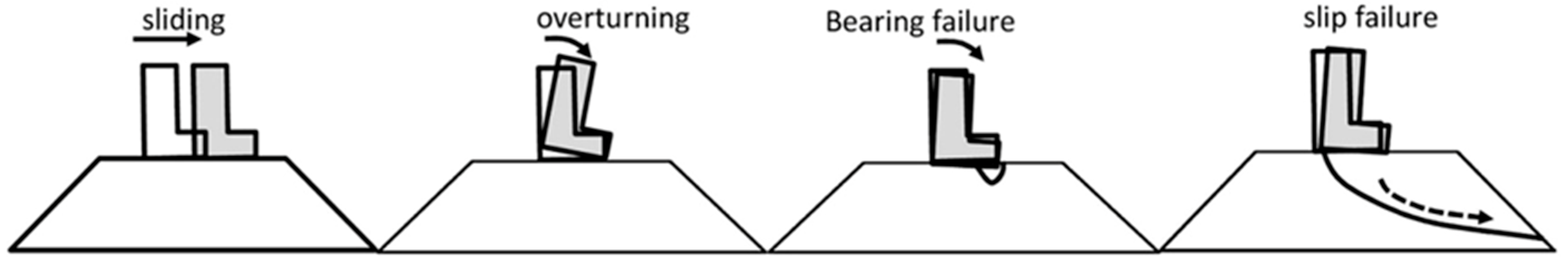
Within the modes of failure of breakwaters, those related to the crown wall are some of the most important. The main and specific ones, which usually are the object of practical calculations, are sliding, rigid and plastic overturning, and bearing capacity of the foundation (Figure 1). Other breakwater modes of failure, such as global geotechnical failure, may affect or be affected by the crown wall [1].

The calculation of these modes of failure is usually done by integrating the instantaneous forces acting against the crown wall, in the consideration of maximum static forces. However, the forces are usually of very short duration, especially in the case of crown walls not fully protected by the slope’s main armor units. The broken wave hits directly against them, generating impulsive pressures depending on the wave’s characteristics and its impact against the structure.

To consider this effect, it is common to truncate the signal obtained in laboratory tests (by pressure cells or by dynamometers) in different ways: by eliminating 1‰ or 2.5‰ of the waves that generate greater loads, by eliminating 1‰ or 0.1‰ of the data records, or other laboratory practices [1,2,3,4]. This is done in order to eliminate some instantaneous data records that, if we considered them, would generate excessively large structures.

For this reason, is convenient to improve the knowledge of the performance of the crown wall and its movements in the time domain by proposing the dynamic calculation of the structure, particularly in cases where impulsive pressures are present [5] and considering the variation of the conditions of the core. Thus, the entire data can be used, even those data that produce instantaneous forces over the static equilibrium conditions, which could generate permissible movements of the crown wall by port operations and that do not produce the failure of the structure.

In the present study, the movements expected by the crown wall of the main breakwater of the outer port of La Coruña in Punta Langosteira are analyzed by using a new proposed simplified model. The structure is subjected to four theoretical load signals (permanent loads, sinusoidal, and two impulsive signals) varying the mechanical characteristics of the foundation. A total of 752 simulations were carried out varying the parameters involved (Young’s modulus and soil model).

2. Proposed Simplified Model

The movement of the crown wall can be estimated by solving the general equation of the dynamics of the rigid solid (see Equation (A1) in Appendix A), with six degrees of freedom (three movements and three turns. However, the analytical resolution of the system becomes very complex [6] and requires, in addition to the knowledge of the instantaneous acting forces, a deep knowledge of the constituent materials of the breakwater; in particular, the core and its characteristics: elasticity, stiffness, damping, permeability, heterogeneity, etc. There are some approximations by numerical model [7,8] that allow point-to-point calculations of the interaction between the structure, the soil, and the water flow inside the breakwater in the time domain. However, the dynamic problems of interacting with an elasto-plastic soil are still not well solved, so in practice, simplifications are proposed for their resolution [7].

The time-domain resolution of the system of equations can be simplified notably by canceling the matrix of damping and introducing two simplifications: on one hand, introducing the damping of the rotation as a response to the deformation existing at the immediately previous instant in the iterative process of calculation; on the other hand, replacing the reaction of the soil to the displacement by the friction in the contact between structure and foundation. The detail of these approximations of the proposed model can be found in Appendix A of this article (see Equation (A15) and Figure A2 in Appendix A). The system of equations can be solved iteratively, so that movements of the crown wall and the deformations of the foundation can be obtained in the time domain. So, the instability or situations incompatible with port operations are determined with enough accuracy.

3. Case Study: Breakwater of Punta Langosteira, Spain

3.1. Breakwater and Crown Wall Description

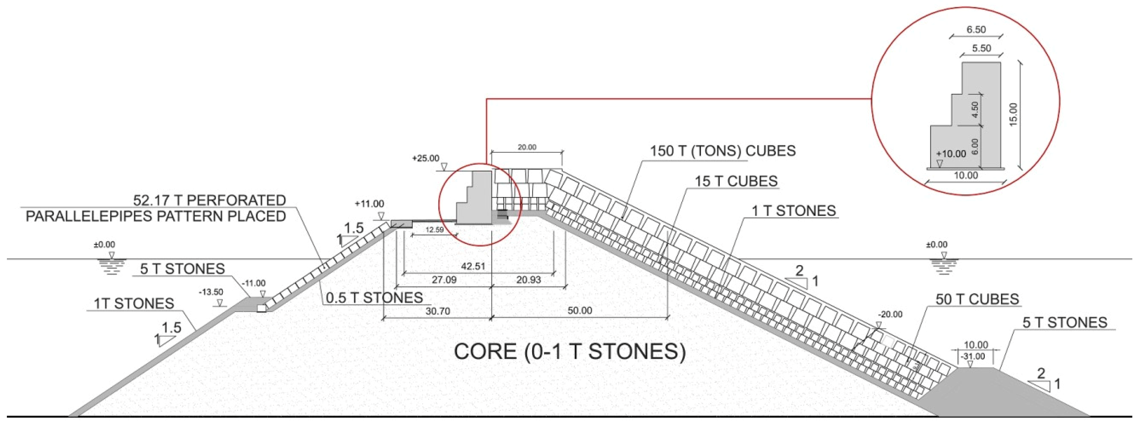
The breakwater of the Outer Port of Punta Langosteira (A Coruña, Spain) is 3.3 km in length, built in a maximum draft of 40 m with respect to lowest astronomical tide (LAT), protected by an armor of two layers of 150 T concrete cubic units of 2.4 T/m³ density, and the slope of the front part is 1 V (vertical):2 H (horizontal) and 1 V:1.5 H in the inner (Figure 2).

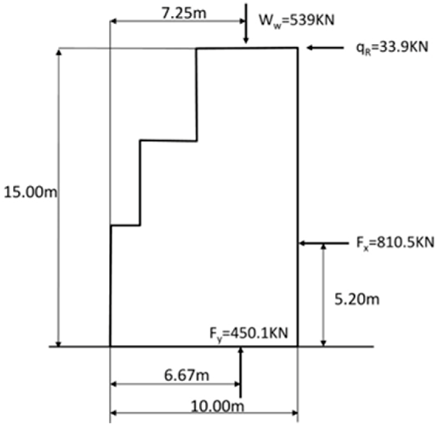
The crown wall rests on the core at +10 m with respect to LAT and is crowned at +25 m over LAT. It is protected in all its height by the main armor of the breakwater and its filters. The crown wall is formed by three solid bodies of different dimensions. The first is 10 m wide at the base and 6 m high; the second is above the first and is 8.5 m wide and 4.5 m high; and the last, above the second, is 5.5 m wide and 4.5 m high. The material of the crown wall is concrete, with a density of 2.37 T/m³, so the mass per linear meter is 275.51 T.

3.2. Soil Mechanics Characteristics

For this study, two models of soil were analyzed to find out the influence of its plasticity:

Elastic model, in which the response of the soil is represented assuming homogeneous, elastic, and isotropic constituent materials, with constant characteristics over time.
- Type of material: gravel and sand;
- Fine fraction granulometry: D_n50 (cm) < 0.10;
- Five Young’s modulus values varying from E (MPa) = 10–400 to analyze the influence of this parameter. The case of an absolutely rigid foundation with an E (MPa) = 27,000 (concrete) is also analyzed;
- Poisson coefficient ν = 0.30 for permanent loads. In the case of pulsating loads, it is considered to be ν = 0.50 [9];
- soil–concrete friction coefficient μ_t = 0.6 (static); μ_d = 0.48 (dynamic);
- soil friction angle θ = 38°.
Elasto-plastic model: in this case, Young’s modulus and shear modules vary depending on the state of loads and the deformation according to a hyperbolic elasto-plastic model of soil response, including the hysteresis of the materials [10,11]. The details of application of the model can be found in Appendix B of this article.

3.3. Loading States

To analyze the performance of the proposed model, the crown wall was tested under three different loading states. One was used to validate the results obtained with the simplified model, and the other two to analyze the different modes of failure of the structure (sliding, overturning, and bearing failure):

Load state A (contrast case): Application of the worse loads determined in the physical model tests (2D large wave flume of the Ports and Coasts Laboratory of the Spanish Public Works Ministry, Madrid, with an active wave absortion system, scale: 1:25) was carried out for the official project [12], obtained for a significant wave height, H_s (m) = 15.1 and peak period, T_p (s) = 20 (Figure 3). A horizontal water load and an overload of the water mass are introduced at the top. The permanent loads against the crown wall due to the pressure of the blocks and materials of the different layers and filters are not considered. The results of the proposed simplified model are compared with the study carried out [13] using the FLAC2D 7.0 code. The worse soil data and parameters obtained by the Ports and Coasts Laboratory of the Spanish Public Works Ministry [14] have been used, taking into account the great variability existing in the functioning of the analysis technique used to determine them.

This load state, although it is demanding, generates high safety coefficients, so limited movements of the crown wall are expected (Table 1).

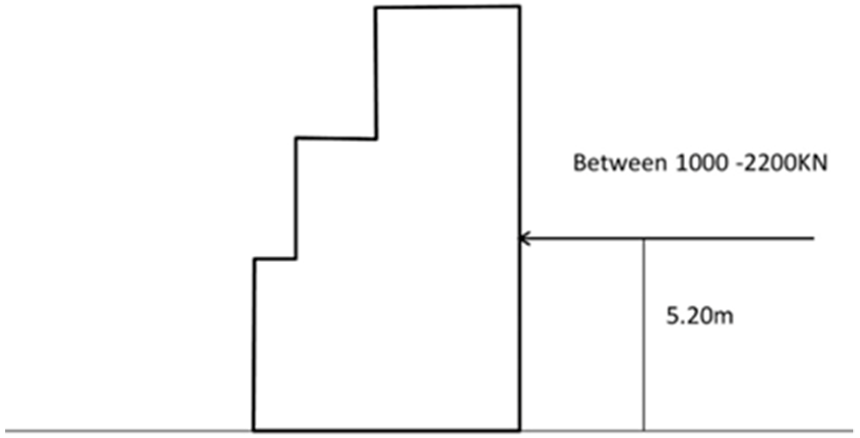
Load state B: This was used to analyze the performance of the structure before the sliding failure. The horizontal load is increased from F_x (KN) = 1000 to 2200 with a determined arm (5.2 m) so that the instability due to overturning does not occur. The existence of vertical sub-pressure loads will not be considered in order to not introduce a component that distorts the slip analysis (Figure 4).

Sliding safety coefficients less than unity are obtained by the application of this load state (Table 2). Thus, by introducing this information in the proposed model, it will be possible to know the influence of the shape of the signal in the time domain and the influence of the characteristics of the core material in this mode of failure.

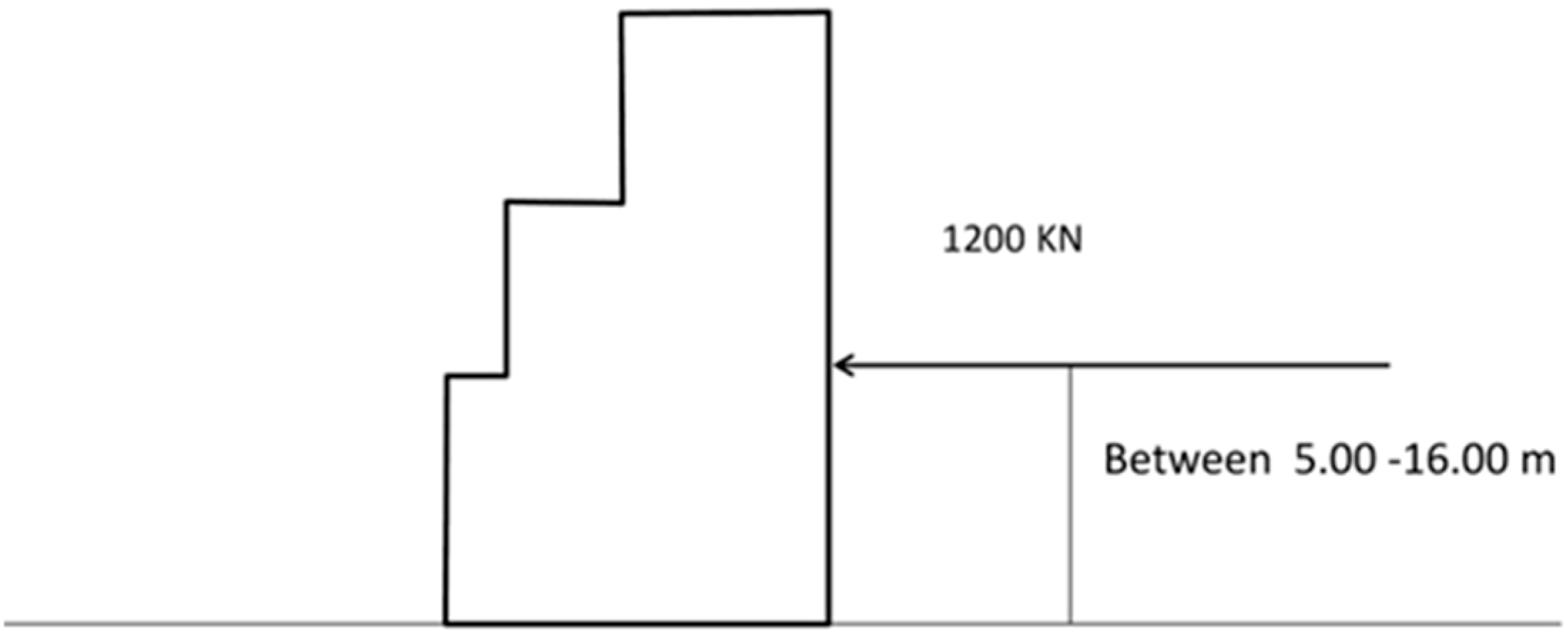
Load state C: This state corresponds to a state of static instability due to overturning and bearing capacity failure of the foundation. Maintaining the horizontal load F_x (KN) = 1200, the application arm is increased from 5 m to 16 m, so that the instability due to overturning occurs. The existence of vertical sub-pressure loads is not considered in order to not introduce a component that distorts the problem of overturning and failure of the foundation (Figure 5).

The bearing capacity safety coefficients obtained by the application of this load state are substantially less than unity (Table 3). Introducing this load state in the proposed simplified model, the influence of the shape of the signal in the time domain and the influence of the characteristics of the core material can be analyzed.

3.4. Shape of the Loading State Signal in the Time Domain

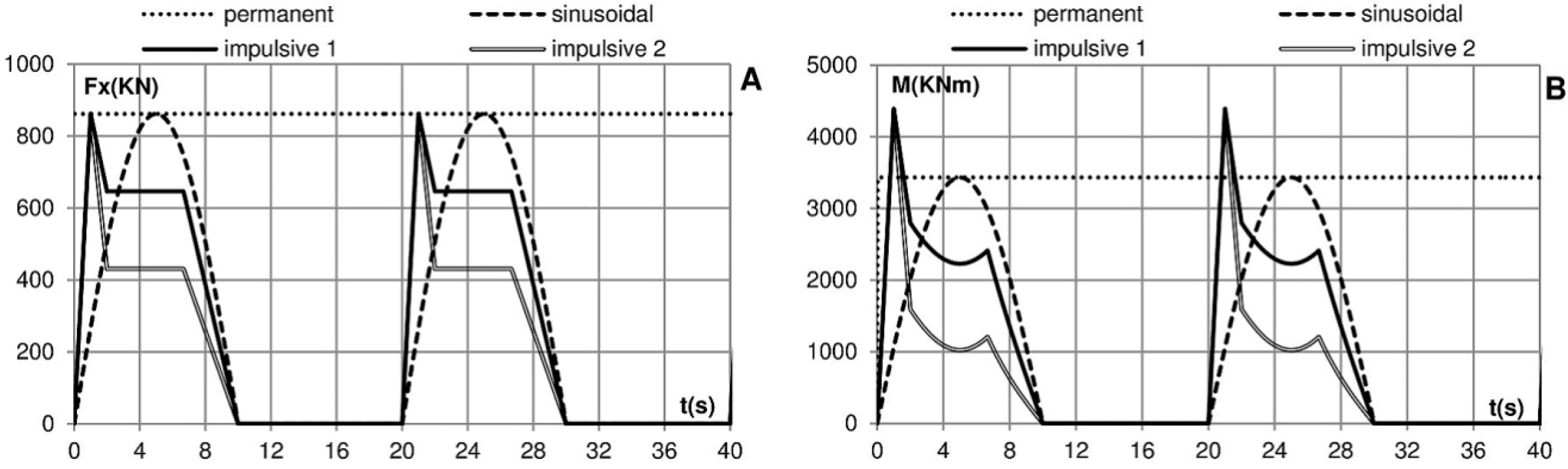
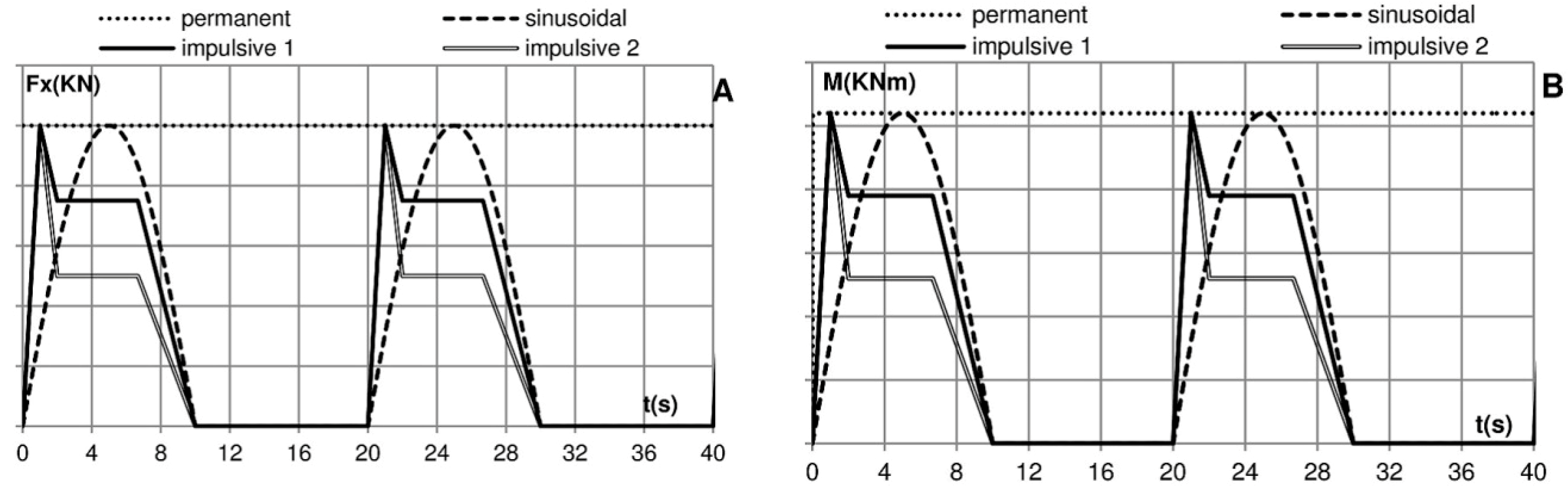
A fundamental aspect for the practical applicability of the model and its sensitivity is the typology of the acting force. Therefore, the performance of the model is analyzed with four different theoretical signals in each of the loading states, with an interval of T(s) = 20, where T—wave period (Figure 6 and Figure 7), and repetition of 10 cycles of loads.

Permanent: The signal (F_x, F_y) is constant and equal to the maximum force.
Sinusoidal: The signal (F_x, F_y) follows a sinusoidal law in a semi-period of the wave with a maximum amplitude equal to the maximum force.
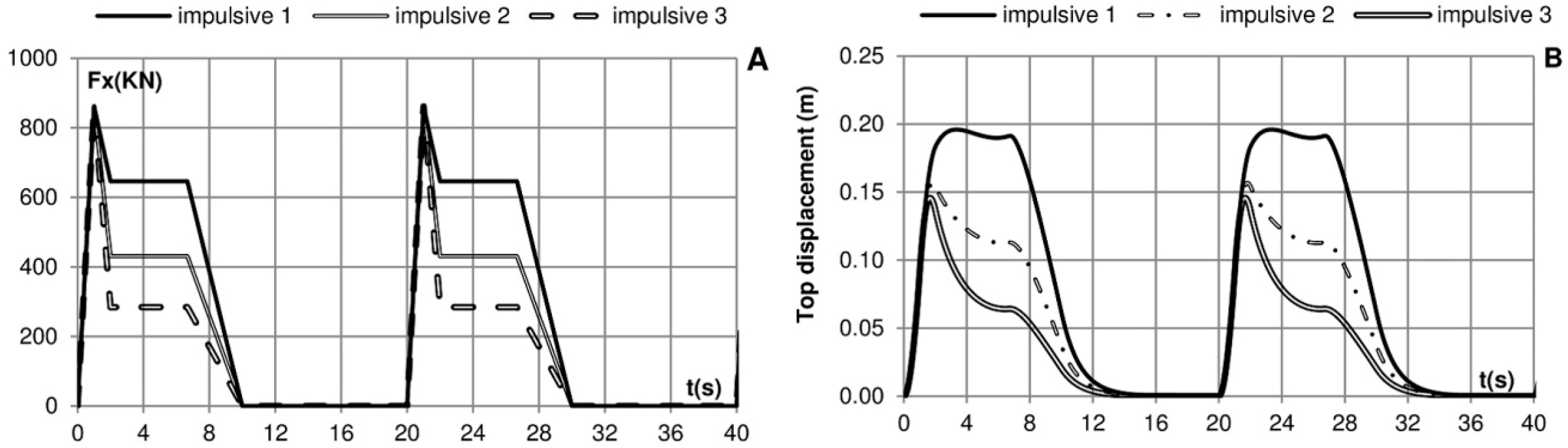
Impulsive 1: The signal for the horizontal force (F_x) presents a maximum equal to the maximum force at a rise time of 0.05 T (1 s), subsequently reducing to 75% and disappearing in a half-period of the wave. With regards to the vertical force F_y, in the case of load state A, a sinusoidal law follows in a semi-period of the wave, with a maximum amplitude equal to the maximum F_y. In the case of loading states B and C, F_y is not considered.
Impulsive 2: Same as Impulsive 1, with a value of 50% for F_x.

The calculation made with the permanent actions is comparable to the static calculation of the crown wall, introducing the mechanic characteristics of the soil as an element that determines the turning movement of the crown wall in adapting to the overturning stress that it experiences. The sinusoidal signal has the shape of a theoretical sine wave. The impulsive actions respond to church-roof signals [1] with impulsive pressures of short duration against the crown wall. These types of signals occur in many cases if there is a direct impact of the wave against the crown wall, in the case that it is not fully protected by the armor. In the first impulsive action defined (tip factor of 1.33), the influence of the impulsive pressure is much less than in the second one (tip factor of 2.0).

4. Results Obtained with the Simplified Model Proposed

4.1. Load State A

A total of 56 simulations were carried out, varying the shape of the loading state signals (4 shapes), the elasticity of the soil (7 elasticity modules), and the model of the soil (2 models).

4.1.1. Elastic Soil

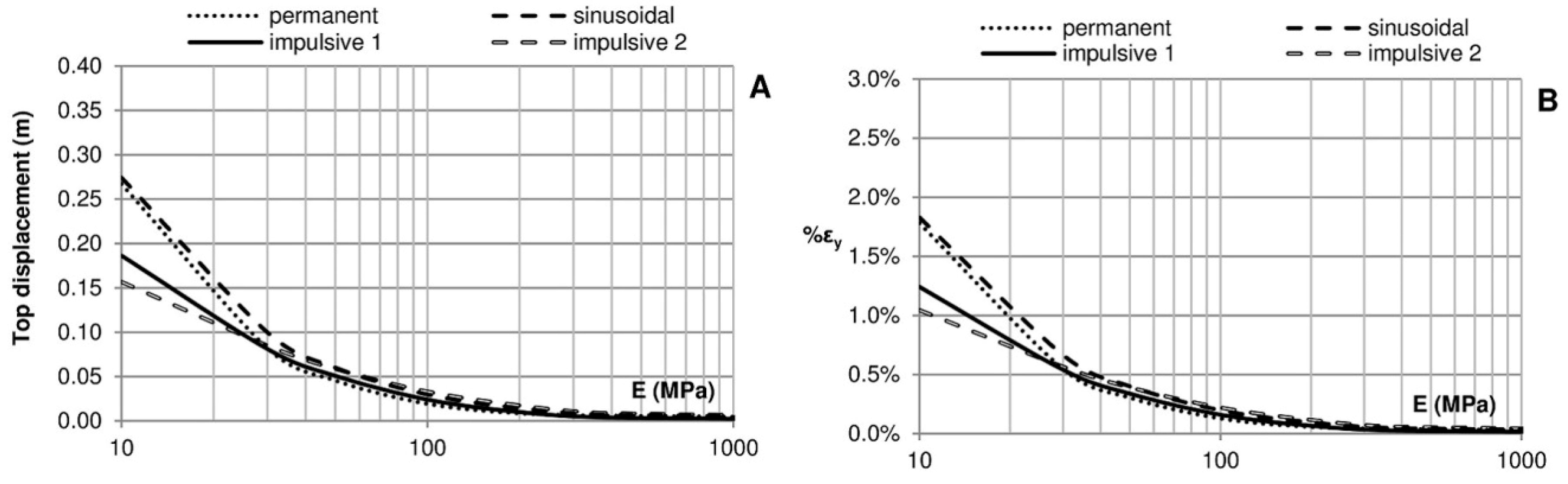
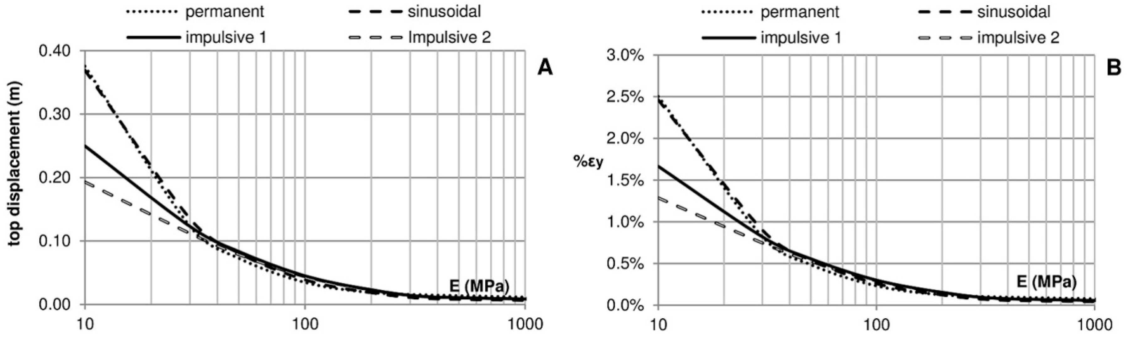
The movements produced on the top have a direct relationship with the modulus of elasticity of the foundation material. At a higher stiffness, a smaller movement corresponds, and vice versa. In Figure 8, the influence of the shape of the signal can be observed. Impulsive actions produce less movement since the maximum forces are of very short duration. This fact is more accentuated in the case of the Impulsive 2 signal with a tip factor of 2.0.

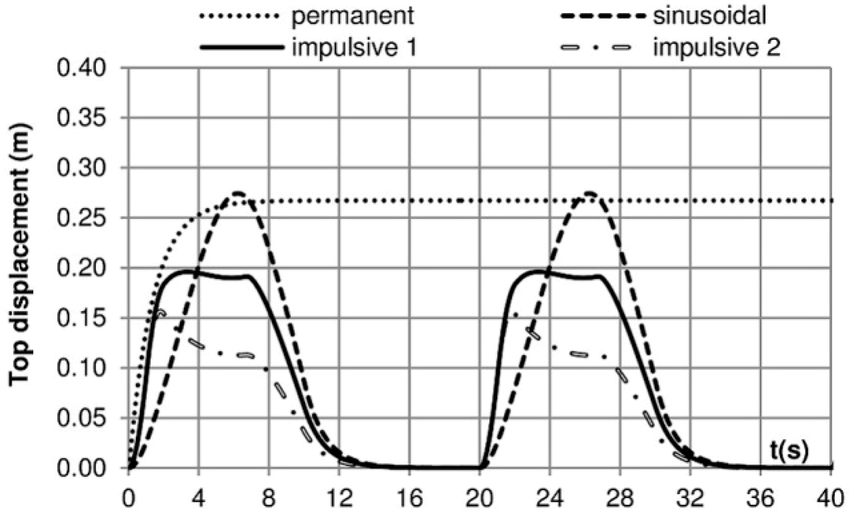
The movements of the top, for the case of E (MPa) = 10, are presented in Figure 9. It can be observed that the maximum movement occurs in the case of sinusoidal acting forces due to the larger Poisson’s coefficient considered in a pulsating loading shape compared with permanent loads. Also, it can be observed that, as Pedersen [2] pointed out, when the tip factor is equal to or greater than 2.0, the constant part of the force has very little relevance in the movement.

The estimated deformations of the foundation are far from those considered inadmissible (See Table A2 in Appendix B). For the values of E (MPa) = 10 and E (MPa) = 100, the maximum deformation does not exceed 2.0% and 0.25%, respectively.

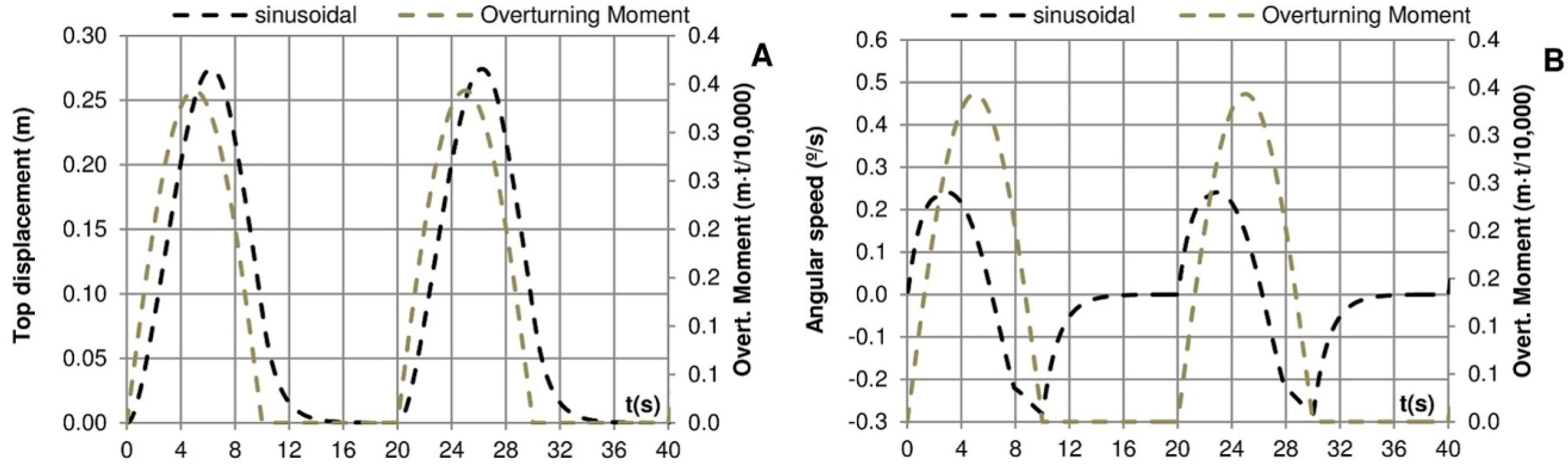
Figure 10 shows the movement on the top and the angular velocity in the time domain obtained with a sinusoidal action, related to the overturning moment. It can be observed that the largest movement occurs with a certain delay in relation to the maximum loading moment. In the case of the sinusoidal signal, in which the maximum loading moment occurs at the instants t (s) = 5 and t (s) = 25, the maximum movement occurs at the values of t (s) = 6.4 and t (s) = 26.4. This delay is produced by the inertia of the movement. In the analysis of the speed, the passing of “0” or change of direction of rotation indicates the point of the maximum amplitude of the movement.

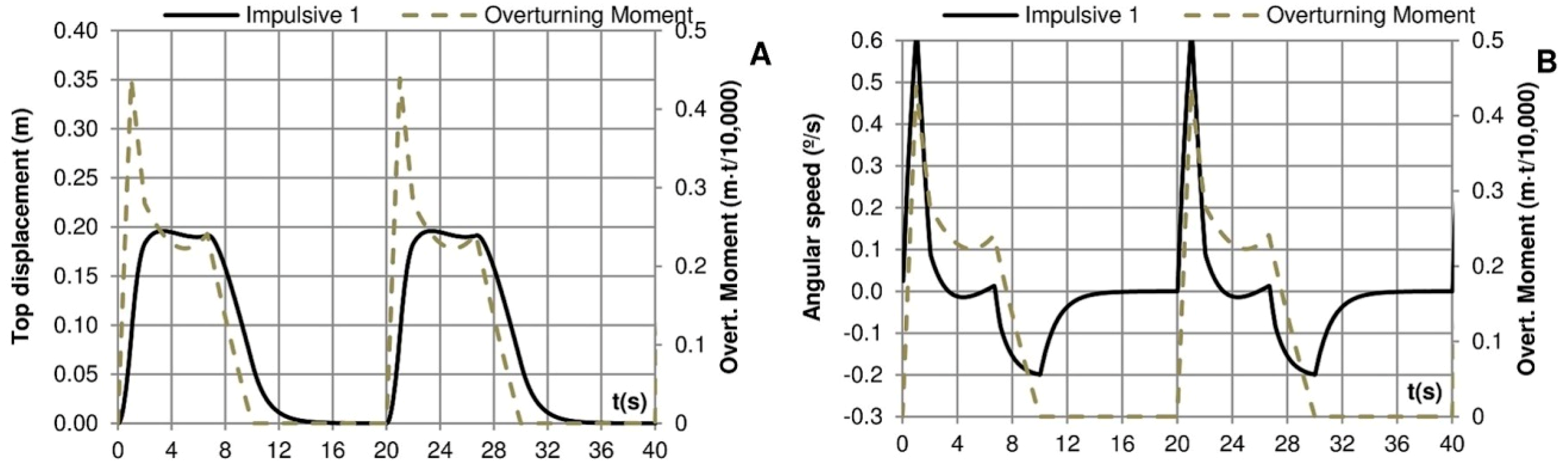
Figure 11 shows the movement on the top and angular velocity of the crown wall for the case of Impulsive 1 (tip factor = 1.33). It is observed that the maximum moment coincides in time with the maximum positive angular velocity. However, throughout the load reduction phase of the impulsive pressure, the crown wall continues to rotate in a positive direction, although the velocity is slowed. The passing of “0”, which coincides with the maximum displacement of the top, occurs in this case once the impulse pressure has finished. This fact causes a reduction of the total movement of the crown wall with respect to the expected one in the case of permanent actions applied, which stabilizes approximately at t (s) = 14 (Figure 9).

4.1.2. Elasto-Plastic Soil

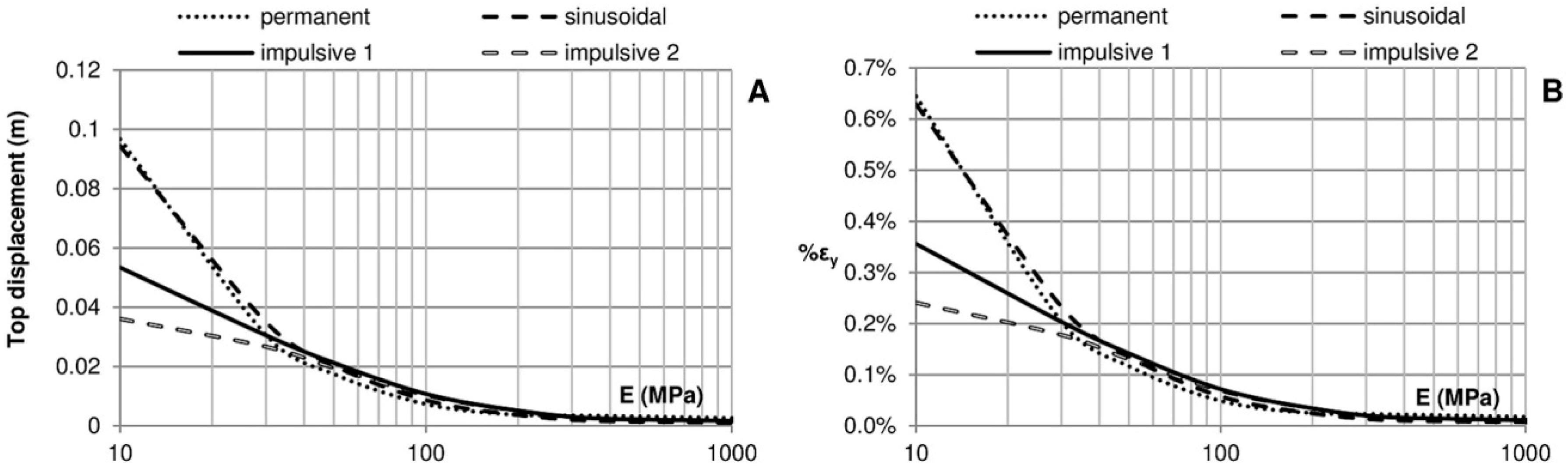
In this section, the influence of model plasticity is analyzed. As in the elastic case, the influence of the load shape on the movement can be observed (Figure 12). However, it can be verified by analyzing Figure 8 and Figure 12 that the movements and deformations in this second case (elasto-plastic) are larger than those in the first (elastic), demonstrating the good performance of the model.

The expected movement in the case of the sinusoidal action is larger than that expected in the case of a permanent load. This fact is derived from the different Poisson coefficients considered in both cases (ν = 0.3 for permanent load and ν = 0.5 for sinusoidal load [9]. On the other hand, the inertia of the movement, produced in the case of cyclic signals, produces a change in the conditions of deformation.

The estimated deformations in the foundation are again far from those considered inadmissible (See Table A2 in Appendix B). In the case of this model of soil, a residual deformation of the foundation between 0.24% and 0.64% occurs as a function of the load signal, as a consequence of the nonlinearity of the stress and deformation (Figure 13).

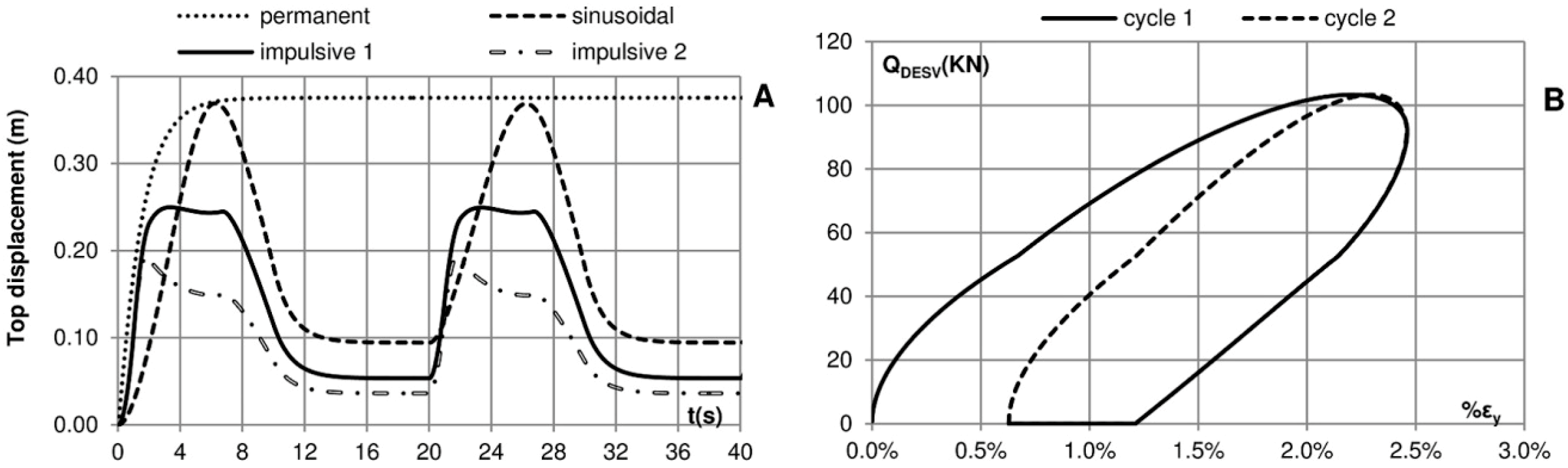
Analyzing the movement that occurs in the first 2 cycles with E (MPa) = 10, for each of the excitation signals, it is observed that there is a residual deformation generated in the first load cycle, which remains until the occurrence of a larger value than that which produced it, according to Atkinson’s model [16]. This fact is more visible in the stress–strain graph of the sinusoidal load, with a vertical residual deformation of 0.64% (Figure 14).

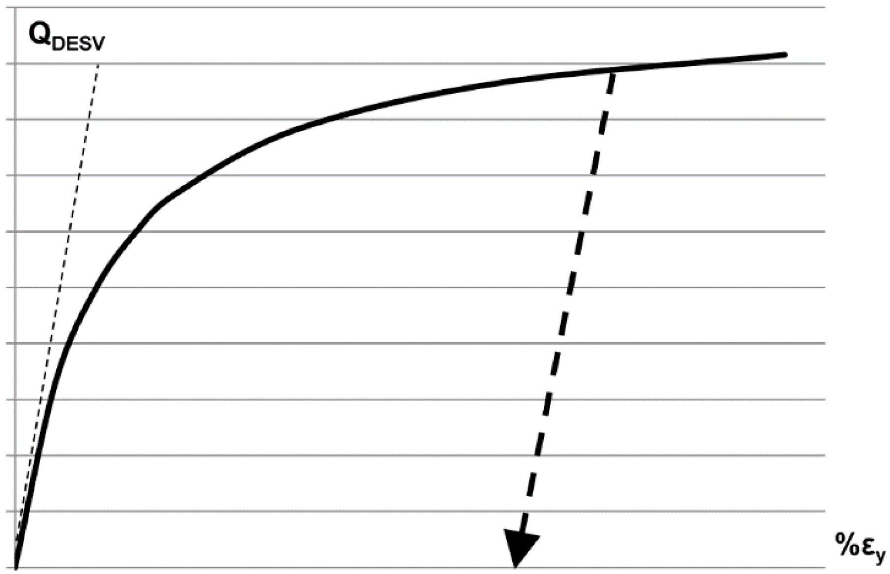
The hardening process of the soil can also be seen in Figure 14. The expected movement is less in the second cycle than in the first one. Due to the consideration of Atkinson’s model [16], the behavior of the soil will be elastic if the load deviator does not increase over the maximum that had occurred (more information about the load deviator (Q_DESV) is provided in Appendix B).

4.1.3. Comparison with FLAC2D 7.0 Code

The results obtained with the simplified model and those obtained with the FLAC2D 7.0 code are presented below (Table 4). Using the model hypothesis made with respect to the damping, no horizontal movements are recorded, since the sliding threshold is not reached (Coulomb hypothesis [17] has been considered: the resistance to the movement over a plane is proportional to the normal force exerted). However, it is verified that net movements of the same order of magnitude are obtained, providing a case for validation of the proposed model.

The comparison with the model FLAC2D 7.0 code considering the maximum possible transverse deformation of the soil (see Equation (A16) in Appendix A) is presented in Table 5:

Again, similar results are obtained, with a small variation in the horizontal deformation for E (MPa) = 10 due to the hypothesis considered.

Even though there are very few data, there has been analyzed the correlation between the displacements of the top of the crown wall obtained using the proposed simplified model and those obtained using FLAC2D code. The correlation obtained is quite good. The root-mean-square error (RMSE) obtained is 0.03 m. The Pearson’s coefficient of correlation is R² = 0.97.

4.1.4. Influence of Tip Factor and Rise Time in the Church-Roof Signals

The tip factor can be larger than 2.5 [3]. There have been used in the calculations two smaller ones because, as the maximum forces and moments were maintained in all shapes of loading state, the use of a larger tip factor should produce a faster decrease in the total movement of the crown walls.

On the other hand, the rise time has also an influence on the dynamic response. Typically, the values obtained in laboratory are in the range of 0.01–0.2 s [2], and in the prototype, in the range of 0.1–1 s [1] (depending on the scale: approximately between 0.01 T_p and 0.1 T_p). In our case, the chosen rise time was equal to 0.05 T in the church-roof signals (Impulsive 1 and Impulsive 2).

To analyze the influence of these two parameters in the performance of the crown wall, its dynamic response was calculated under three additional church-roof theoretical signals:

Impulsive 3: Same as Impulsive 1, with a value of 33% for F_x;
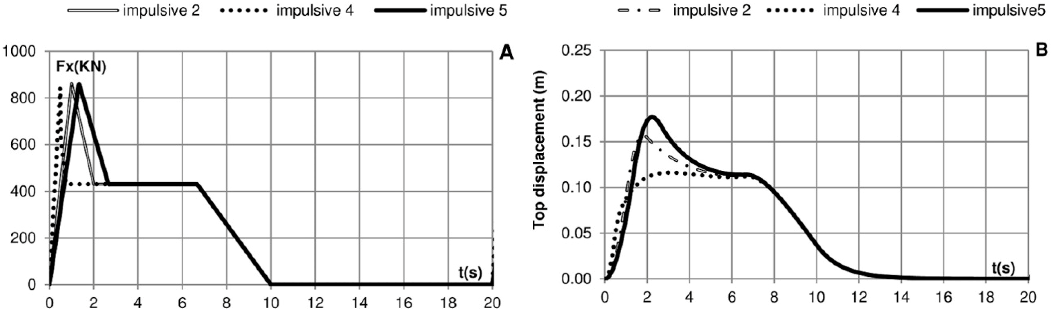
Impulsive 4: Same as Impulsive 2, with a rise time of 0.025 T (0.5 s);
Impulsive 5: Same as impulsive 2, with a rise time of 0.075 T (1.5 s).

The influence on the dynamic response of tip factors can be seen in Figure 15. It can be observed that the reduction in the flat part of the signal has a large influence on the movement of the structure. As stated by Pedersen [2], if the tip factor is larger than 2.0, the constant part of the wave loading following the peak has little influence on the dynamic response.

The influence of rise time on dynamic response can be seen in Figure 16. It can be observed that, if the rise time is reduced from 0.075 T (Impulsive 5) to 0.025 T (Impulsive 4), the maximum movement of the crown wall is also reduced. This effect is produced due to the inertia of the structure. The movement is very fast at the beginning in the case of Impulsive 4 (0.025 T). Then, when the impulse stops, the movement continues, but it does not reach the maximum of Impulsive 2 or 5.

In these theoretical signals, there is no reproduction of other kinds of impulses that could occur in the prototype or in the laboratory. However, the peak force generated by the impact of the wave crest could be followed by other force oscillations due to the air pockets entrapped within [1]. These oscillations could be in the range of the natural period of oscillation of the structure and could amplify its movement.

4.2. Load State B

The influence of soil mechanics and the shape of the loading state in sliding were studied in the analysis of load state B.

A total of 336 simulations were carried out, varying the forces acting against the crown wall (7 horizontal forces), the shape of the loading state signal (4 shapes), the elasticity of the soil (6 elasticity modules), and the model of the soil (2 models).

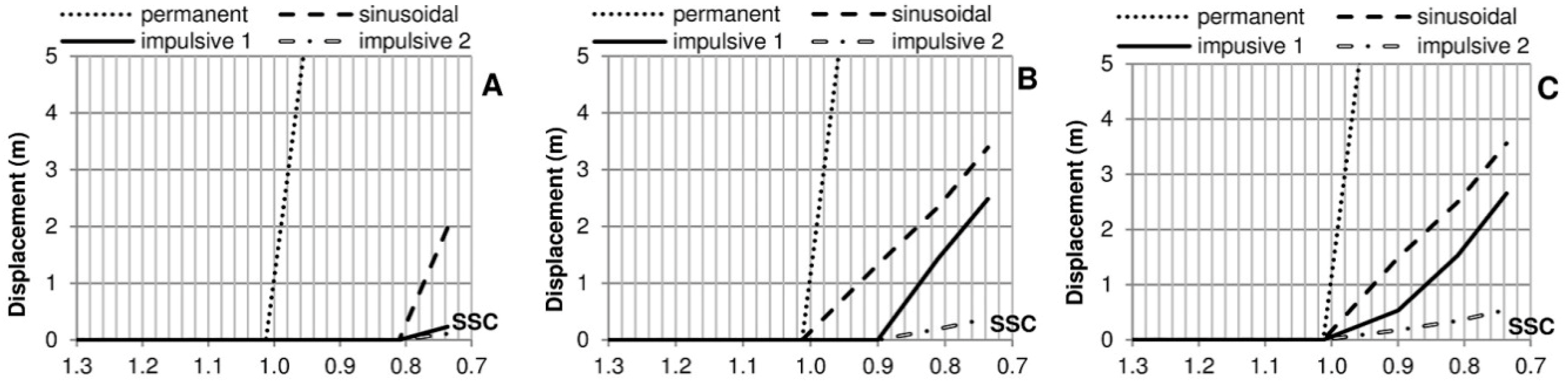
Figure 17 shows the sliding of the crown wall, considering an elastic soil foundation in each of the four excitation forces as a function of the sliding safety coefficient for different Young’s modulus values of the soil.

In the case of permanent loads, the situation can be assimilated to the static calculation where the crown wall begins to slide and the safety coefficient is less than 1.0. On the other hand, the displacement produced is the same, being independent of the soil characteristics. Therefore, these factors do not influence sliding in the static calculation.

In the case of a very rigid foundation, such as the crown wall resting directly on concrete (E (MPa) = 27,000), or even with values of E (MPa) > 400, the displacement occurs whenever the static equilibrium situation is exceeded, whatever the shape of the action. This result is especially important and is a central element of the present study, since it is verified that in these cases, the calculation must be made using the maximum impulsive pressures recorded without truncating the laboratory or other data records (Figure 17). The reason for this performance is that, when the safety coefficient factor falls below 1.0, there is not any absorption of energy in the foundation soil, and all the wave energy is used to “move” the crown wall. Further, when the movement begins, the friction coefficient is reduced dramatically.

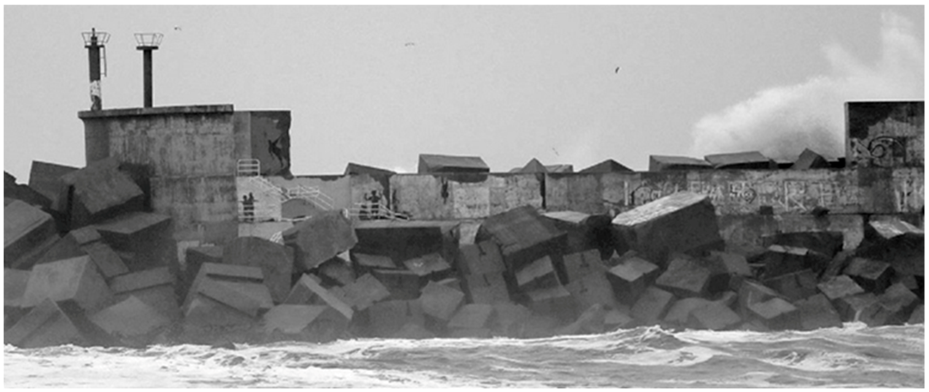
This type of breakage is very common in crown walls that can be stable as a whole, constructed over the core of the breakwater that behaves as a dumping absorber of the movement. However, the upper parts, if they are not joined to the rest of the body of the crown wall, could become unstable. Figure 18 shows a breakage of this type in the breakwater of A Garda (Spain) in February 2017. Other cases have occurred in recent years, particularly in locations in the north and northwest of Spain.

For the rest of the signals analyzed the less rigid the soil, the smaller the expected sliding of the crown wall. Moreover, the applied horizontal load could exceed the static equilibrium conditions without starting the sliding. This is because although the soil is deformable, the horizontal impulse is initially transformed into rotation and, later, into displacement. If the duration of the load that exceeds the static equilibrium condition is very small, the crown wall does not mobilize and it recovers the original position in the load reduction phase.

The influence of the load type of signal on crown wall sliding has been compared for 3 different Young’s modulus values (Figure 19). It can be verified that in the case of very rigid soil (E (MPa) = 27,000), in all cases, the sliding starts if the sliding safety coefficient (SSC) is less than 1.0. On the other hand, it has been proved that regardless of the type of soil, in the case of permanent loads, the sliding occurs if the load exceeds the static equilibrium conditions (SSC < 1), reflecting the good performance of the proposed simplified model. Likewise, it can be observed that if the soil has a certain flexibility, in the case of impulsive loads, sliding may not occur even with SSC less than 1.0.

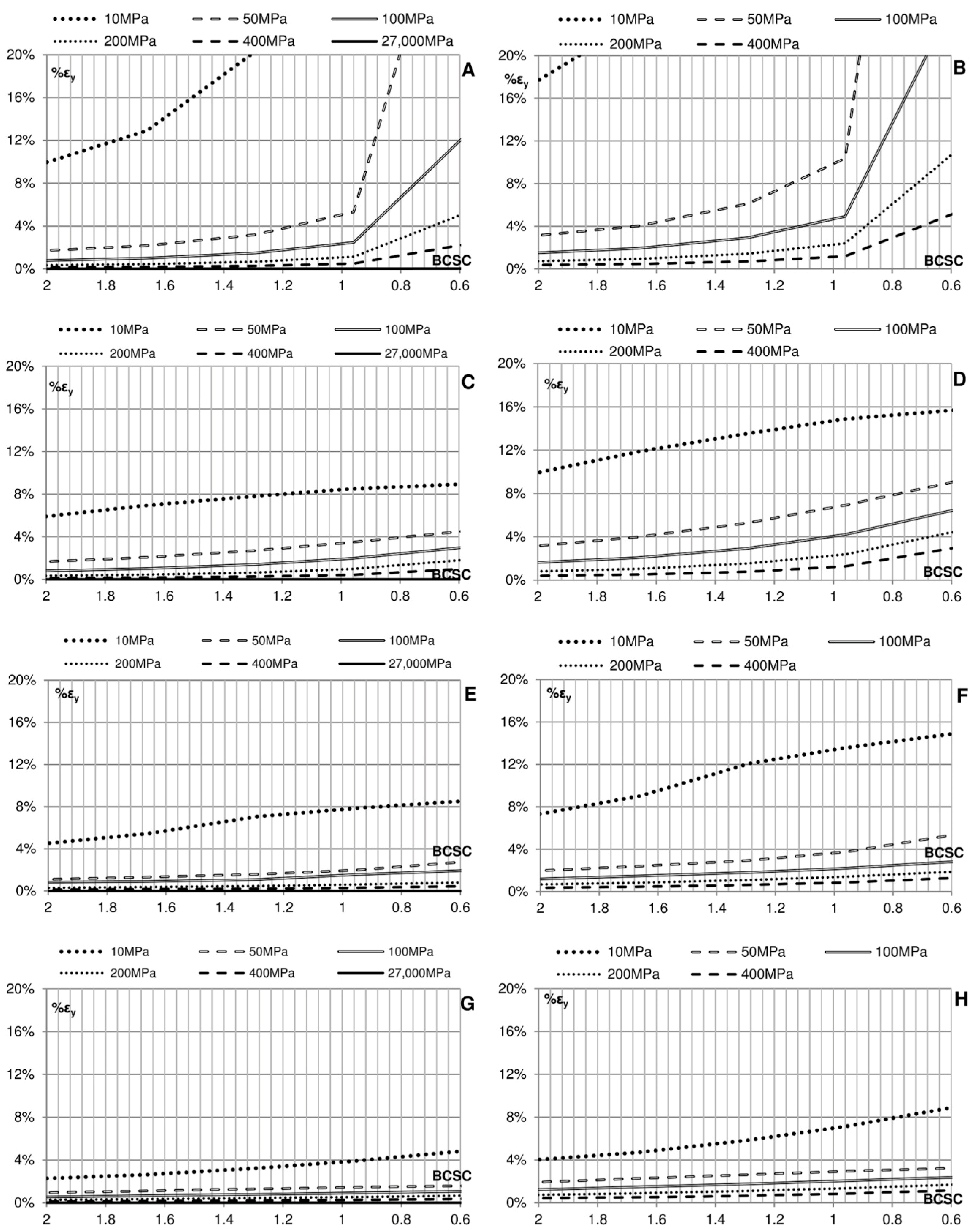
Comparing the results obtained for load state B with the bearing capacity safety coefficient (BCSC) obtained (Figure 20), it can be deduced that, independently of the amplitude of the deformations, especially in the case of the soil with E (MPa) = 10, the soil does not collapse (See Table A2 in Appendix B). In the case of this loading state, the failure of the structure occurs by sliding.

Table 6 presents, for the load state B, the sliding occurring after 10 cycles of load for each of the simulations and each of the signal shapes. It can be seen that in the case of a Young’s modulus above E (MPa) = 400, if the sliding condition is exceeded (SSC < 1.0), displacement of the crown wall occurs. However, in the case of more flexible soils, depending on the load shape, the sliding condition can be overcome without displacement of the crown wall (e.g., for E (MPa) = 100 with SSC = 0.90, sliding does not occur in the case of impulsive loads). In the case of very rigid foundations (E (MPa) = 27,000), the elasto-plastic soil model was not considered.

However, the collapse of the soil did not occur in any of the simulations. Table 7 shows the results for the vertical deformation. It can be seen that the limit of deformation is not exceeded in any of the cases (See Table A2 in Appendix B).

Table 8 shows the modes of failure produced in the simulations carried out with the load state B and the corresponding sliding and bearing capacity safety coefficients calculated at the time of failure. It can be seen that in the case of soils with a certain flexibility and different signal shape than permanent loads, sliding safety coefficients could be less than 1.0 without resulting in sliding. However, for rigid soils, failure always occurs with a sliding safety coefficient equal or less than unity (SSC ≤ 1.0).

4.3. Load State C

The influence of soil mechanics and the shape of the loading state in overturning were studied in the analysis of load state C.

A total of 360 simulations were carried out, varying the forces acting against the crown wall (9), the shape of the loading state signal (4 shapes), the elasticity of the soil (5 elasticity modules), and the model of the soil (2 models).

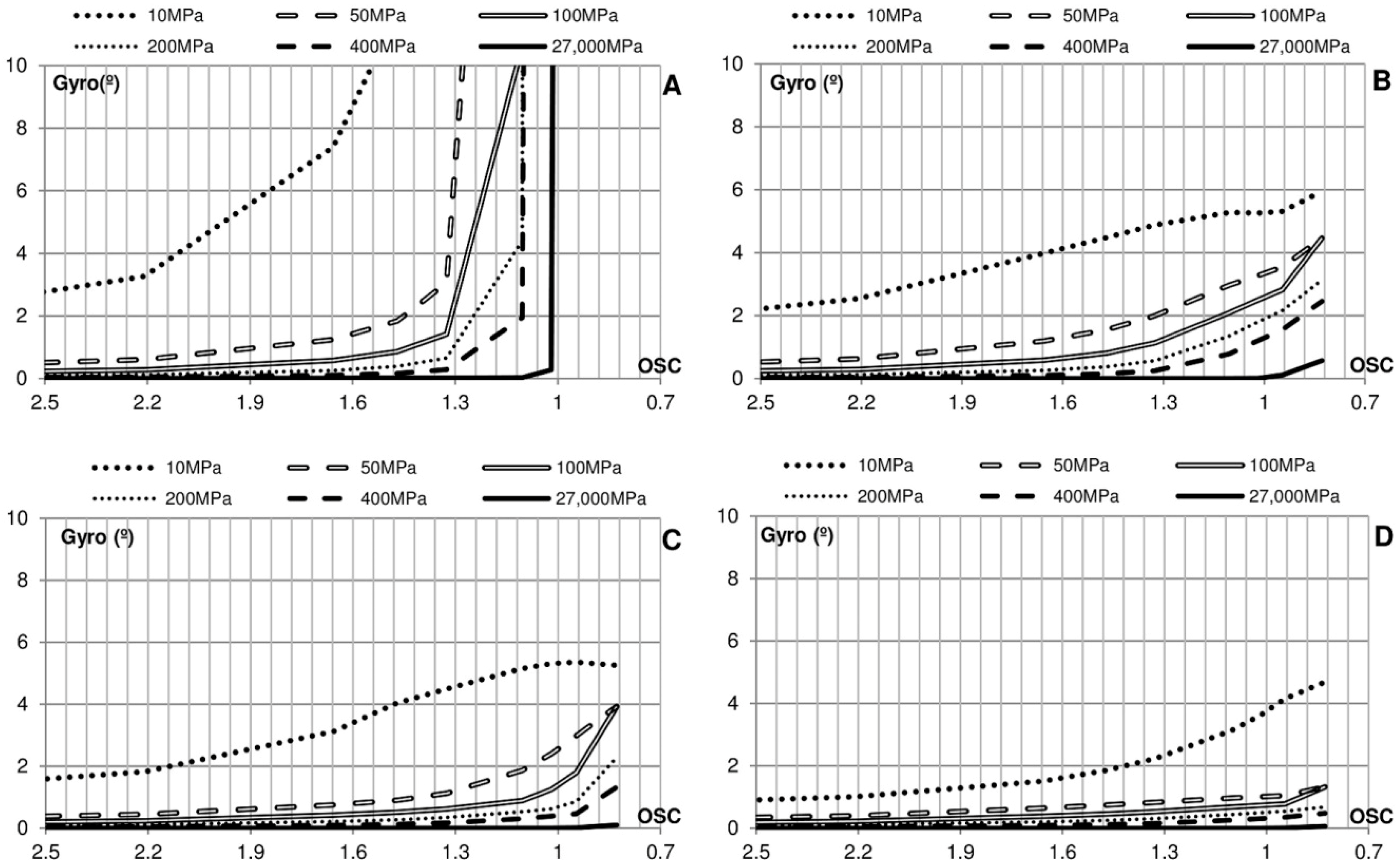
Figure 21 shows, for the load state C with each signal shape and type of soil, the turning of the crown wall in relation to the overturning safety coefficient (OSC) of the structure. It can be seen that, in the case of permanent loads and similar to static calculation, if the foundation has a very low Young’s modulus, turning occurs in initial stages of the loading, reaching instability with lower loads. However, for very rigid soils, the instability occurs with OSC values close to 1.0 (OSC ≈ 1.0). It is also highlighted that for other signal shapes, the crown wall may have OSC values less than 1; however, the turning of the structure could be acceptable. For example, in the case of Impulsive 2, even for materials with E (MPa) = 50, the rotation produced with a OSC of 0.8 is less than 2°.

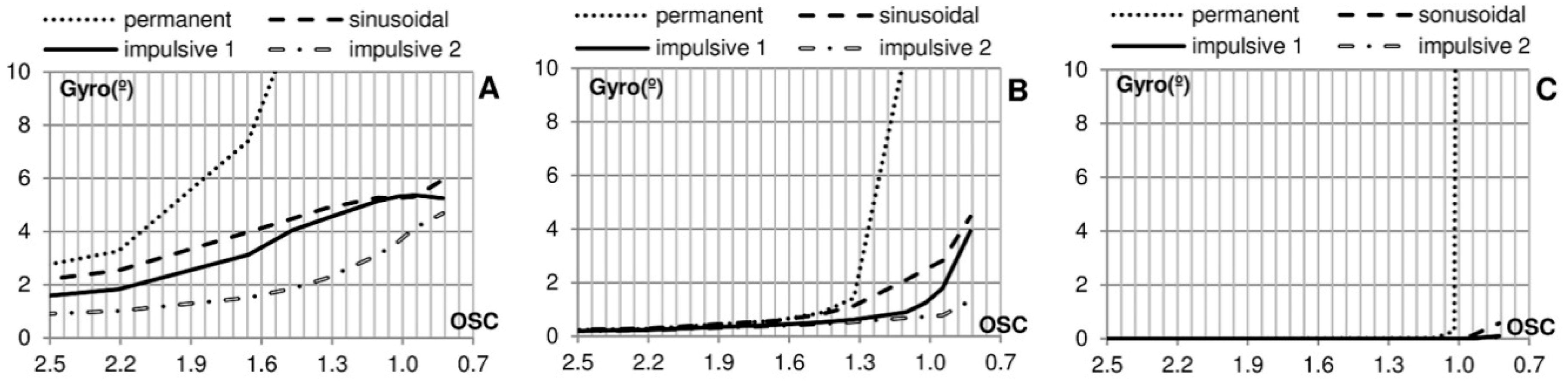
The influence of the loading signal shape on the crown wall rotation has been analyzed (Figure 22). It can be verified that in the case of very rigid soil (E (MPa) = 27,000), until the OSC is less than 1.0 (OSC < 1.0), the crown wall does not begin to turn. At that time, in the case of permanent loads, the structure failure occurs immediately. However, in the other load types, the crown wall does not fail because the signal duration is not enough to cause the total instability of the structure. With deformable soils (e.g., E (MPa) = 10 and E (MPa) = 100), in the case of permanent loads, the failure of the structure occurs for values of OSC larger than 1.0. Also, if the soil has a certain flexibility in the case of impulsive loads, overturning may not occur even with overturning safety coefficients smaller than 1.0.

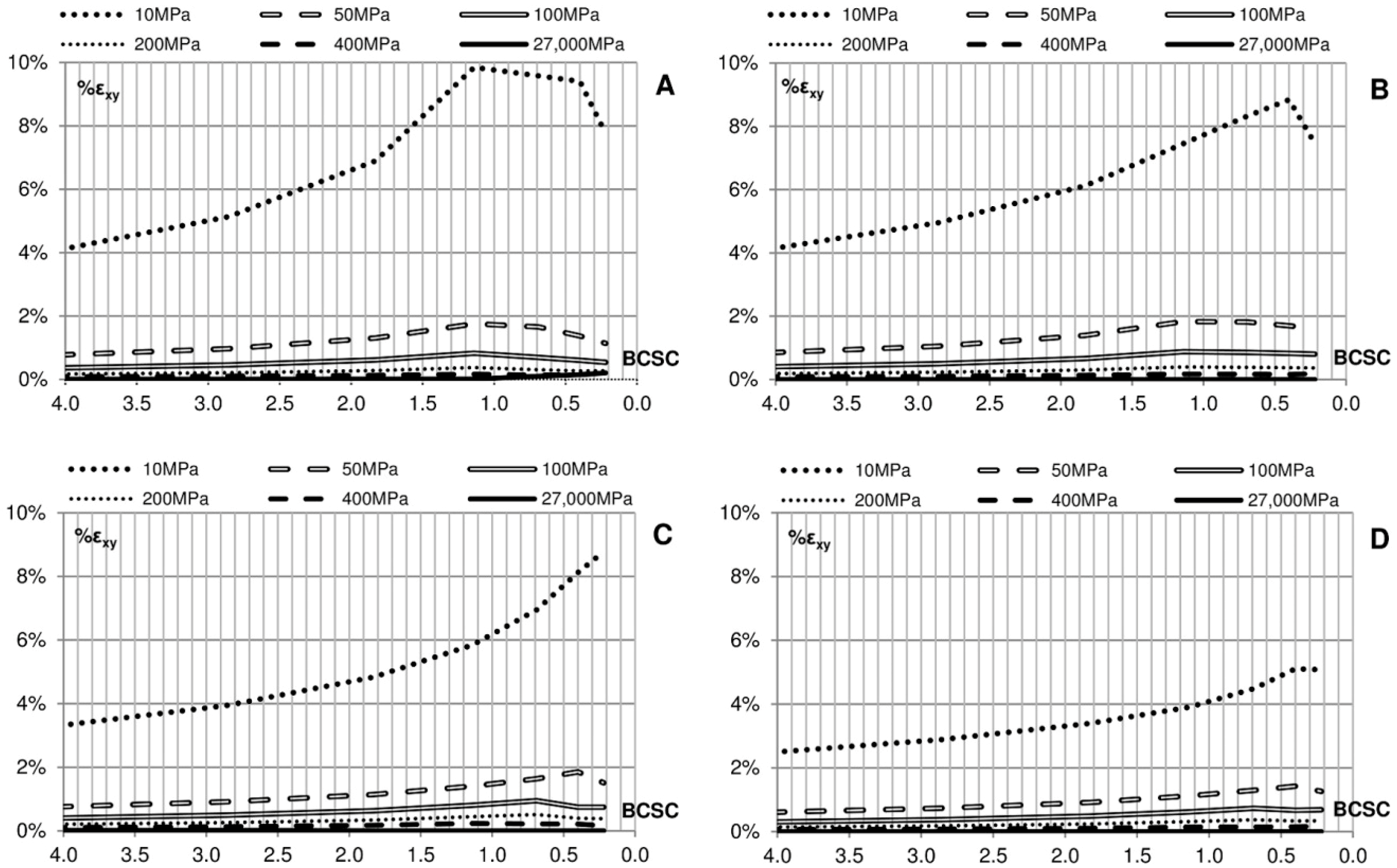
In Figure 23, the deformation of the foundation related to the bearing capacity safety coefficient (BCSC) is presented. For the four signal shapes and the two types of soils (elastic and elasto-plastic) studied, it can be seen that in the case of permanent load (static calculation), the maximum deformation of the foundation exceeds the maximum acceptable defined value for BCSC; i.e., greater than 1.0. Only in the case of E (MPa) = 27,000 (concrete), the maximum allowed deformation is not exceeded, even with safety coefficients close to 0.0. In this case, the section fails due to rigid overturning, not plastic. In impulsive loads with a bearing capacity safety coefficient lower than 1.0, the maximum acceptable deformation is not exceeded. On the right side of Figure 23, the deformations for elasto-plastic soils are presented, showing larger deformations than in the case of elastic soil.

Table 9 shows the turning of the crown wall in degrees for both elastic and elasto-plastic soils, indicating the overturning and bearing capacity safety coefficients. As expected, before the failure due to rigid overturning occurs, the structure fails due to bearing capacity of the foundation (except in the case of E (MPa) = 27,000, for which this has not been considered). In the case of E (MPa) = 27,000 and permanent loads (static calculation), the failure due to rigid overturning occurs when the overturning safety factor is <1.0. Also, it can be observed that the shape of the signal has a decisive influence on crown wall failure. In the case of impulsive pressures and elastic soil, the failure does not occur. Likewise, in the case, both of permanent and sinusoidal loads with elastic soil, the bearing capacity safety condition can be overcome (BCSC < 1.0) and the collapse of the foundation does not occur. Moreover, for elasto-plastic soil and impulsive signals, the deformations of the foundation may become unacceptable (See Table A2 in Appendix B) when the rigidity of the soil increases.

Table 10 shows the modes of failure produced in the simulations carried out for load state C and the corresponding bearing capacity and overturning safety coefficients at the time of failure. It can be observed that the failure of the structure always occurs due to the foundation bearing capacity, except in the case of E (MPa) = 27,000 (concrete), in which the failure occurs due to overturning. In certain cases of impulsive signals, the failure occurs with bearing capacity safety coefficients below unity. In some cases, the crown wall did not fail. For example, in the case of E (MPa) = 100, with permanent loads, the maximum acceptable deformation is reached for OSC = 1.32 and BCSC = 0.95 (for elastic soil), and OSC = 1.50 and BCSC = 1.36 (for elasto-plastic soil). In the case of sinusoidal load, maximum acceptable deformation is reached for OSC = 1.22 and BCSC = 0.66 (for elastic soil), and OSC = 1.51 and BCSC = 1.36 (for elasto-plastic soil); and in the case of Impulsive 1 load, for OSC = 0.97 and BCSC = 0.01 (for elastic soil), and OSC = 1.20 and BCSC = 0.61 (for elasto-plastic soil). It is remarkable that the maximum acceptable deformation for Impulsive 2 load is not reached.

5. Conclusions

This study presents a simplified model for the dynamic calculation of breakwater crown walls, providing results of the relative movements expected based on hydrodynamic forces and soil characteristics (elastic, elasto-plastic). The proposed simplified model gives a first estimation of crown wall stability, comparing the displacement and rotation for certain designs, regardless of their structural stability, and whether they are compatible with the defined operating conditions.

The model has been validated in a real case, the main breakwater of the Outer Port of Punta Langosteira (A Coruña, Spain), by means of its comparison with the numerical model FLAC 2D 7.0. The good performance of the model proposed was verified with static calculation (permanent loads) and elastic soil in a range of Young’s modulus values (E (MPa) = 10–27,000), producing sliding and rigid overturning whenever the safety coefficients were less than 1.0. The usual modes of failure of the crown walls were found to be the sliding and the bearing capacity of the foundation. However, rigid overturning only takes place in case of absolutely rigid foundations (E (MPa) = 27,000).

A fundamental aspect of the study was the decisive importance of the shape of the loading state signal. Four different shape of loads were analyzed. The results show that the impulsive forces of short duration may not transmit enough energy, regardless of its intensity, to cause a failure of the structure, even with safety coefficients less than unity obtained by static calculation.

The importance of the Young’s modulus of the soil was also investigated. The analysis shows that with sufficiently flexible foundations, the soil becomes an absorber of the movement, allowing the structure to turn (and its subsequent recovery). However, if the crown wall is based on a very rigid soil or foundation (e.g., concrete), the impulsive forces can be decisive and causes the failure of the structure regardless of their limited duration. This is likely to be the cause of numerous recent crown wall breakages recently found in the upper parts which are not full protected by the main armor of the breakwater slope, in the north coast of Spain (Bermeo, A Garda, Cariño, Malpica). Therefore, it is recommended to carry out a soil-type sensitivity analysis.

The plasticity of the soil was found to be very important. The residual deformations reached in certain loading states can lead to the maximum deformation states in subsequent load stages being exceeded. It seems advisable to always carry out a double analysis: on one hand, assuming elastic soil, which provides information on the rhythmic movement of the structure and its possible resonance; and on the other hand, assuming elasto-plastic soil to determine the residual deformations of the soil and to incorporate the influence of the hysteresis of the foundation materials.

Another important aspect for the design of crown walls found in this study is that the truncation of the pressure signal registered in laboratory tests, [to eliminate a percentage of waves (e.g., 1‰) or a specific number of data registered (e.g., 0.1‰)], must be carried out with caution. This is relevant to avoid the omission of impulsive combinations potentially harmful to the structure. The proposed simplified model allows the use of the complete series of data and check the expected movements of the crown wall and its compatibility with the established design criteria.

Author Contributions

Conceptualization, E.M.; methodology, E.M.; formal analysis, E.M., E.P., J.S. and A.F.; writing—original draft preparation, E.M., E.P., J.S. and A.F.; writing—review and editing, E.M., E.P., J.S. and A.F.

Funding

This research received no external funding.

Acknowledgments

The authors give special thanks to the Port Authority of A. Coruña, Spain, for allowing access to data of the project of the New Breakwater at Punta Langosteira.

Conflicts of Interest

The authors declare no conflict of interest.

Appendix A. Simplified Problem Approach

The movement of the crown wall can be estimated by solving the general equation of the dynamics of the solid rigid (Equation (A1)), with six degrees of freedom (three movements and three turns):

M \ddot{x} + D \dot{x} + Kx = F (t)

(A1)

where M represents the matrix of the masses, D that of damping, and K that of stiffness. The resolution of this system requires, in addition to the knowledge of instantaneous acting forces, the data of the constituent materials of the breakwater, mainly its core (elasticity, stiffness, damping, permeability, heterogeneity, etc.). In an analytical form, the resolution becomes very complex and requires a simplification of the system in order to address it. On the other hand, it can be solved by means of the use of codes to calculate point-to-point iterations between the structure, the soil, and the acting mass of water in the time domain. It also must consider the flow inside the breakwater. However, the dynamic problems posed by interacting with a plastic soil are still not well solved, which is why in practice, there are proposed simplifications for solving them, both in materials and in forces.

This system of complex second-order differential equations can be simplified for a simple analytical resolution with the use of common software codes that allow iterative calculations.

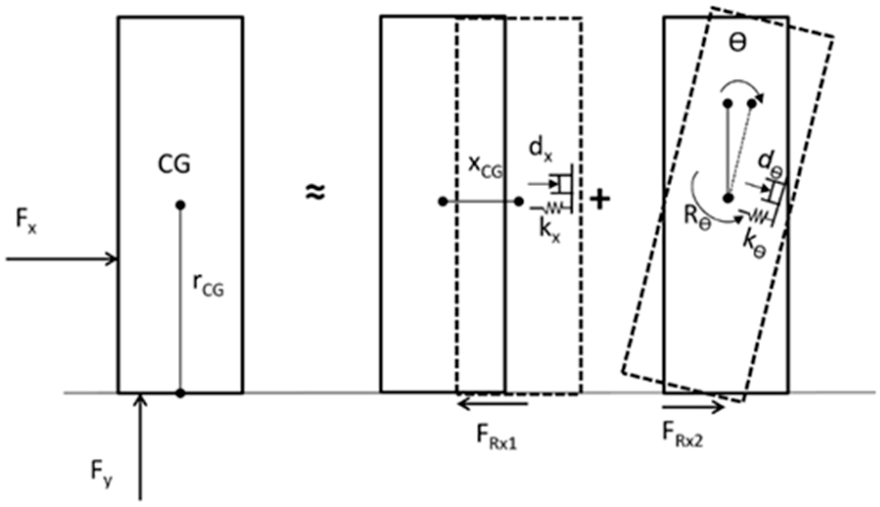
First, a simplification of the movement system is assuming that there are no movements in the vertical and transverse directions and that the rotations are limited to those produced with respect to a transverse axis (Figure A1). The simplified system is limited to the problem of the motion of translation and that of the oscillation, becoming a system of two second-order differential equations with two unknowns. The terms involving “d” represent the damping of the soil, and the terms involving “k” the soil stiffness [2] (Equation (A2)):

\begin{matrix} [\begin{matrix} m & 0 \\ 0 & I_{CG} \end{matrix}] [\begin{matrix} {\ddot{x}}_{CG} \\ \ddot{θ} \end{matrix}] & + [\begin{matrix} d_{x} & - d_{x} r_{CG} \\ - d_{x} r_{CG} & d_{θ} + d_{x} r_{CG}^{2} \end{matrix}] [\begin{matrix} {\dot{x}}_{CG} \\ \dot{θ} \end{matrix}] + [\begin{matrix} k_{x} & - k_{x} r_{CG} \\ - k_{x} r_{CG} & k_{θ} + k_{x} r_{CG}^{2} \end{matrix}] [\begin{matrix} x_{CG} \\ θ \end{matrix}] \\ = [\begin{matrix} F_{x} \\ M_{CG} \end{matrix}] \end{matrix}

(A2)

where m—crown wall mass, x_CG—movement of the centre of gravity, M_CG—turning moment related the centre of gravity, I_CG—inertia moment related to the centre of gravity, r_CG—distance from the centre of gravity to the turning point, d_θ and d_x—damping of the foundation, and k_θ and k_x—stiffness of the foundation.

Figure A1. Crown wall movements. Adapted from the system proposed by Pedersen [2].

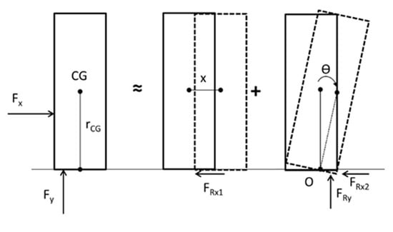
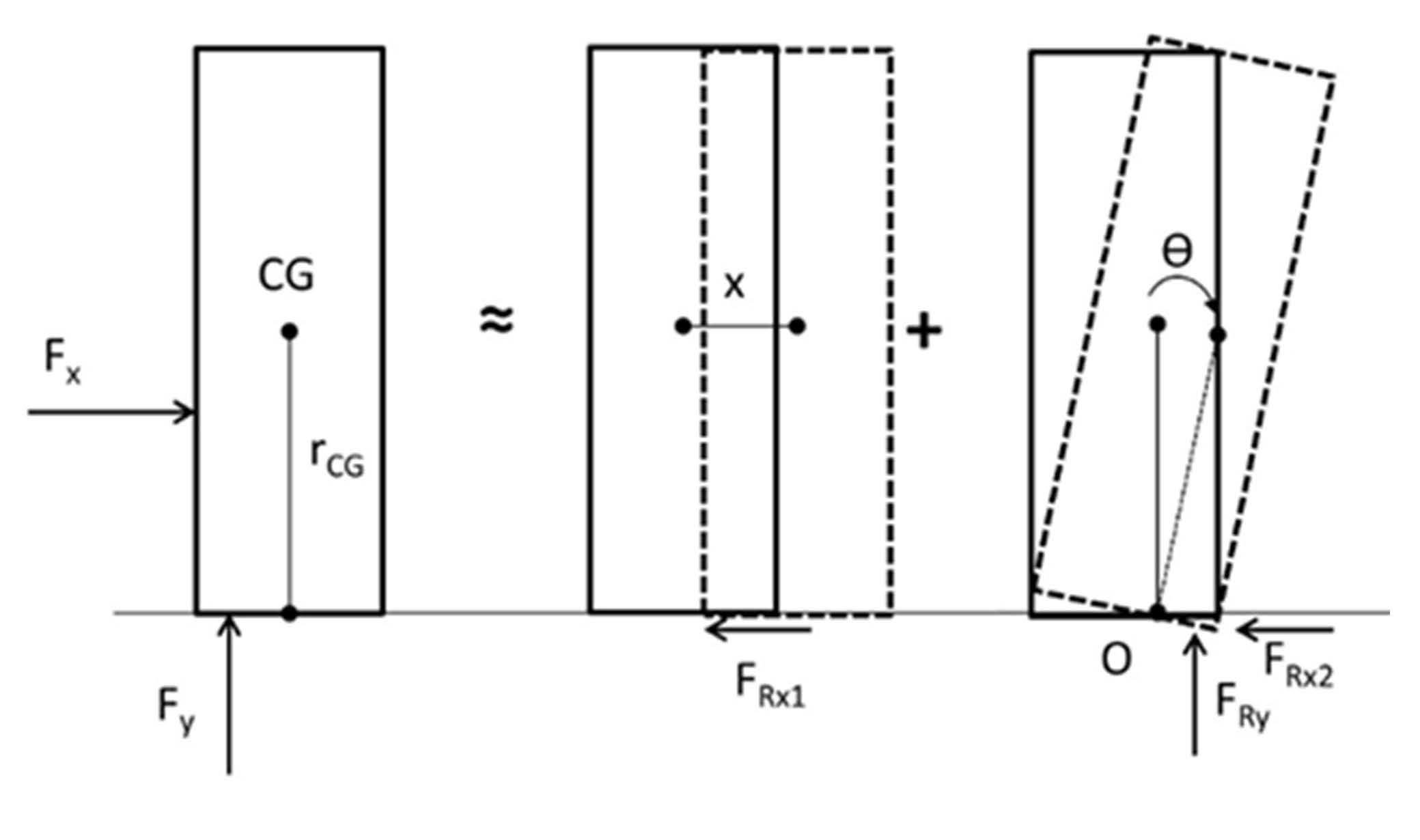
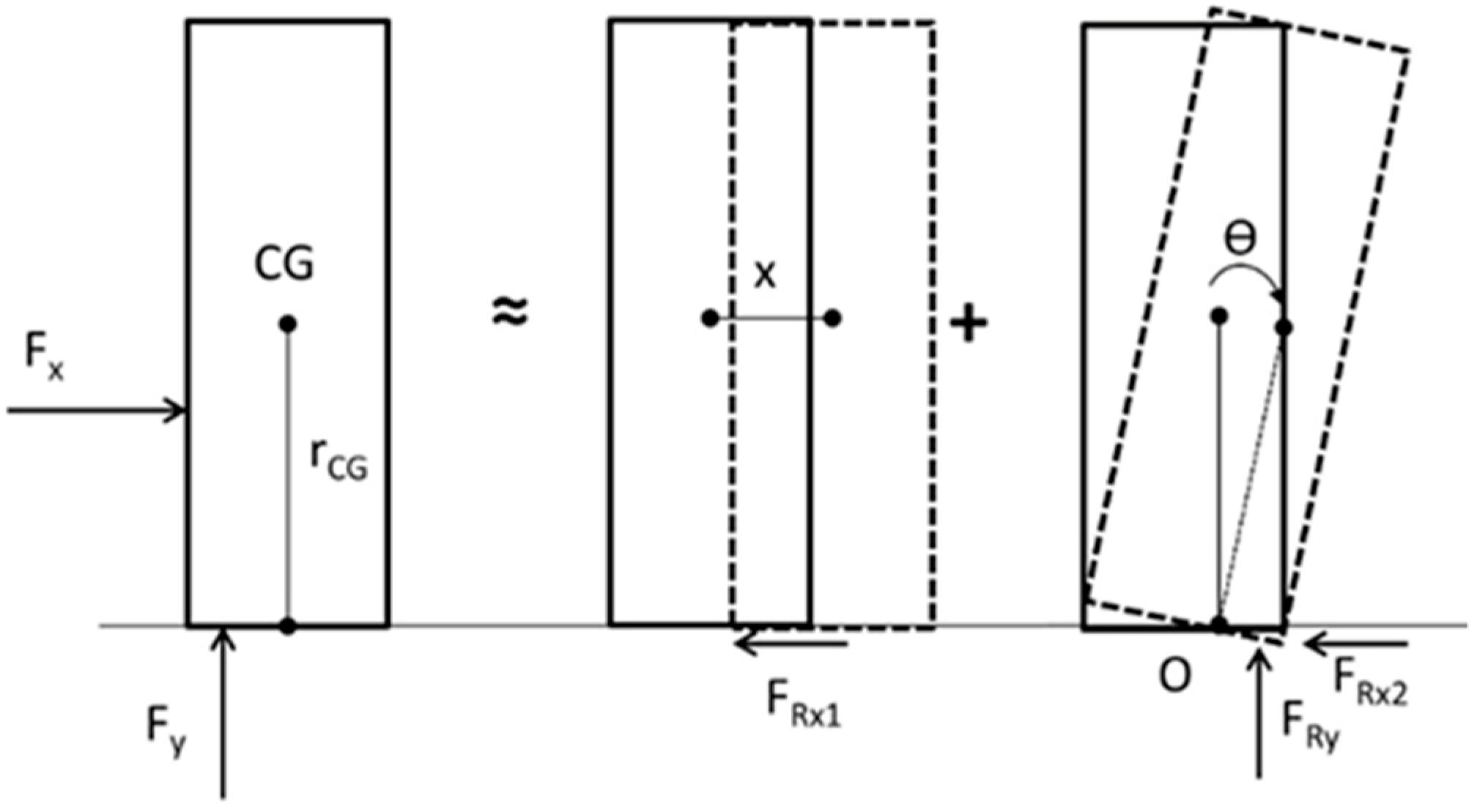
In a second approach, considering that the crown wall rotates with respect to an “O” point of its contact with the soil (Figure A2 and Figure A3), the system can be analysed in a more simplified form (Equation (A3)). Thus, the equations can be expressed as:

[\begin{matrix} m & 0 \\ 0 & I_{O} \end{matrix}] [\begin{matrix} \ddot{x} \\ \ddot{θ} \end{matrix}] + [\begin{matrix} d_{x} & 0 \\ 0 & d_{θ} \end{matrix}] [\begin{matrix} \dot{x} \\ \dot{θ} \end{matrix}] + [\begin{matrix} k_{x} & 0 \\ 0 & k_{θ} \end{matrix}] [\begin{matrix} x \\ θ \end{matrix}] = [\begin{matrix} F_{x} \\ M_{O} \end{matrix}]

(A3)

where M_O—overturning moment related the point “O” of turn, I_O—inertia moment related to the point “O” of turn, x—movement of the crown wall, and ϴ—rotation of the crown wall.

Figure A2. Scheme proposed of the dynamic system. (CG—centre of gravity; r_CG— radio of rotation of the center of gravity, ϴ—gyro; and F_R—resistance of the soil to the movement).

Appendix A.1. Soil Stiffness

It is proposed to estimate the soil stiffness as a function of the deformation through the application of the loads.

Appendix A.1.1. Stiffness against Turning

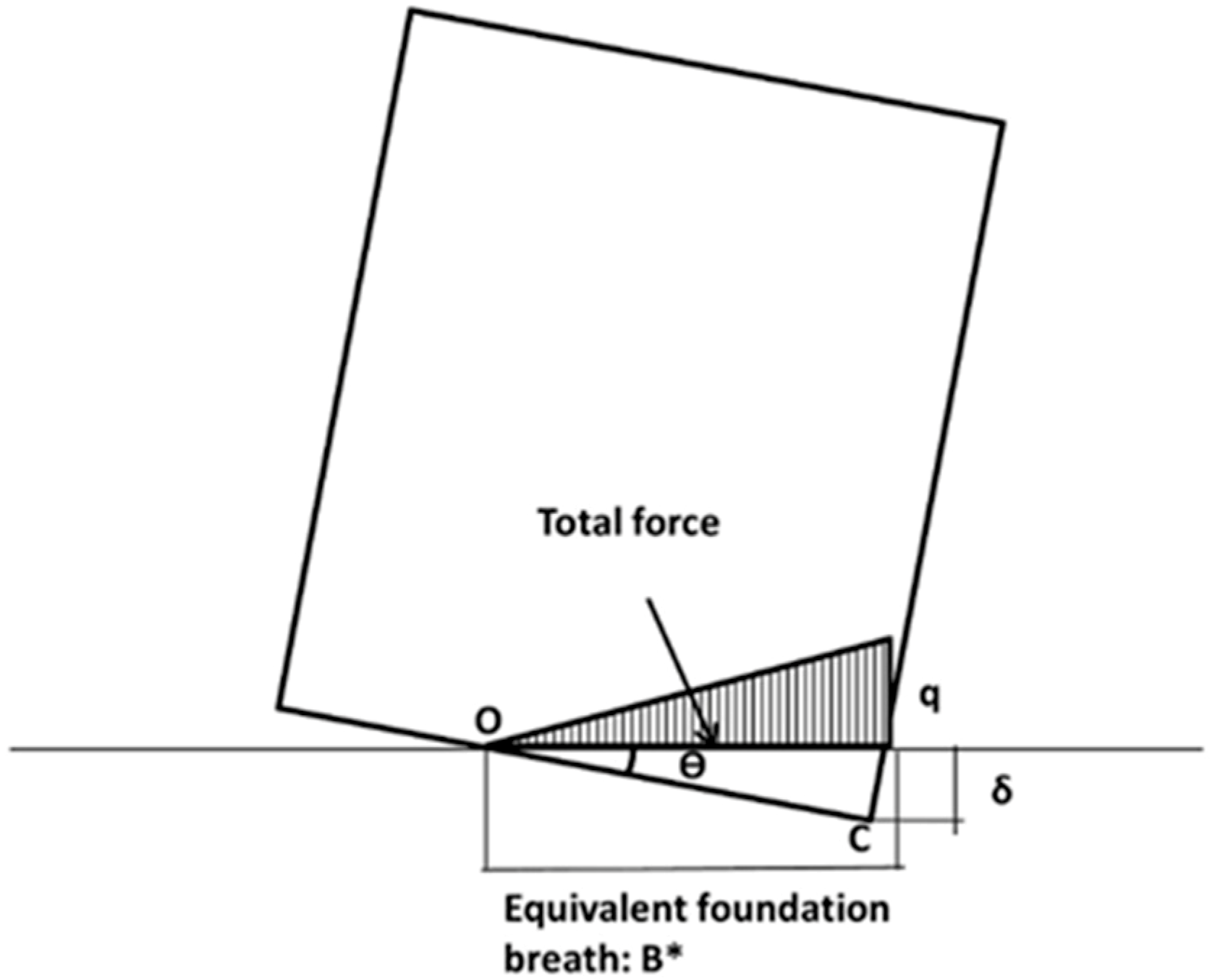
In the previous simplification, it was considered that the crown wall turned around an “O” point located at the contact with the soil. As an approximation, it is suggested that the distance from said point “O” to the inner corner of the crown wall, “C”, which is variable over time, is equal to the active area of contact between the crown wall and foundation (B*) and double that of the distance between the point of application of the resultant forces in that contact plane and the inner corner “C” (called the equivalent foundation breath [5,18]; see Figure A3).

Figure A3. Definition of equivalent foundation breath.

On the other hand, considering the soil as an elastic medium and that the distribution of the loads transmitted to the soil (which depends on its stress-deformational state) is known and has a triangular shape, a vertical movement δC is generated at the point “C”. This parameter is a function of the Young’s modulus of elasticity (E) and the Poisson’s coefficient of the soil (ν), which with a permanent load, can be considered as follows [17] (Equation (A4)):

δ_{C} = (q (1 - υ^{2}) B^{*}) / π E = B^{*} θ \to {qB}^{*} = {π E θ B}^{*} / (1 - ν^{2})

(A4)

Therefore, given that

M_{{Def}_{V}} = k_{θ} θ = ({qB}^{*}^{2}) / 3 = [({π EB}^{*}^{2}) / (3 (1 - ν^{2}))] θ

, the soil stiffness for a permanent load, depending on the angle of rotation of the structure, could be assimilated as such:

k_{θ} = ({π EB}^{*}^{2}) / (3 (1 - ν^{2}))

(A5)

Gazetas [19] proposed a lower stiffness in the case of strip foundations with a layer of incompressible soil at a depth “D” under cyclic loads (Equation (A6)):

k_{θ} = [({π EB}^{*}^{2}) / (4 (1 - ν^{2}))] (1 + 0.1 B^{*} / D)

(A6)

Appendix A.1.2. Stiffness against Movement

The same assumptions made in the previous case can be applied here, considering the soil as an elastic medium and that the distribution of the loads transmitted to the soil is known. So, the movement of the soil, δ_x, as a consequence of the application of a permanent horizontal load in the previous point “C” can be considered [17] (Equation (A7)):

δ_{x} = [(Bq (1 + ν)) / π G] (lnB / 2 - lnB)

(A7)

where B—width of the crown wall, G—shear modulus of the soil

Therefore, given that

q = k_{x} δ_{x} = (π G) / [B (1 + ν) (lnB / 2 - lnB)] δ_{x}

, the soil stiffness for a permanent horizontal load, as a function of horizontal movement, can be expressed as:

k_{x} = π G / [B (1 + ν) (lnB / 2 - lnB)]

(A8)

where the shear modulus of the soil “G”, related to the elasticity Young’s modulus and Poisson coefficient, is considered with the following expression (Equation (A9)):

G = E / (2 (1 + ν))

(A9)

Gazetas [19] proposed a larger stiffness in the case of strip foundations with a layer of incompressible soil at a depth “D” under cyclic loads (Equation (A10)):

k_{x} = [(2.1 G) / (2 - ν)] (1 + B / D)

(A10)

Appendix A.2. Consideration of the Damping of the Movement

The damping of the movement due to the stiffness and viscous characteristics of the foundation can be approached as a response to the instantaneous deformation of the foundation (as a consequence of the punctual stresses in the crown wall at the instant immediately before).

Appendix A.2.1. Damping Corresponding to the Turn

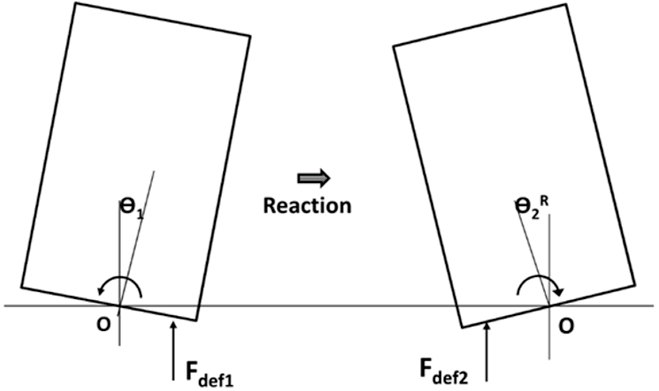
The damping is introduced as an opposite turn to that produced by the turning moment caused by the soil’s reaction to its deformation up until the previous moment (Figure A4).

Figure A4. Damping of the turn due to soil reaction. (F_def—resistance of the soil to deformation produced by the rotation).

Since

M_{{Def}_{V 1}} = I_{O} \ddot{θ_{2}^{R}} + M_{{Def}_{V 2}}

, then, as an a approximation,

θ_{2}^{R} ~ (k_{θ_{1}} θ_{1} t^{2} / 2) / (I_{O} + k_{θ_{2}} t^{2} / 12)

. So, the net rotation at instant “i” is the turn of the loading state in the instant “i” minus the rotation produced by the soil reaction in the instant “i − 1”:

θ_{i_{net}} = θ_{i} - θ_{i - 1}^{R}

(A11)

Appendix A.2.2. Inertial Damping

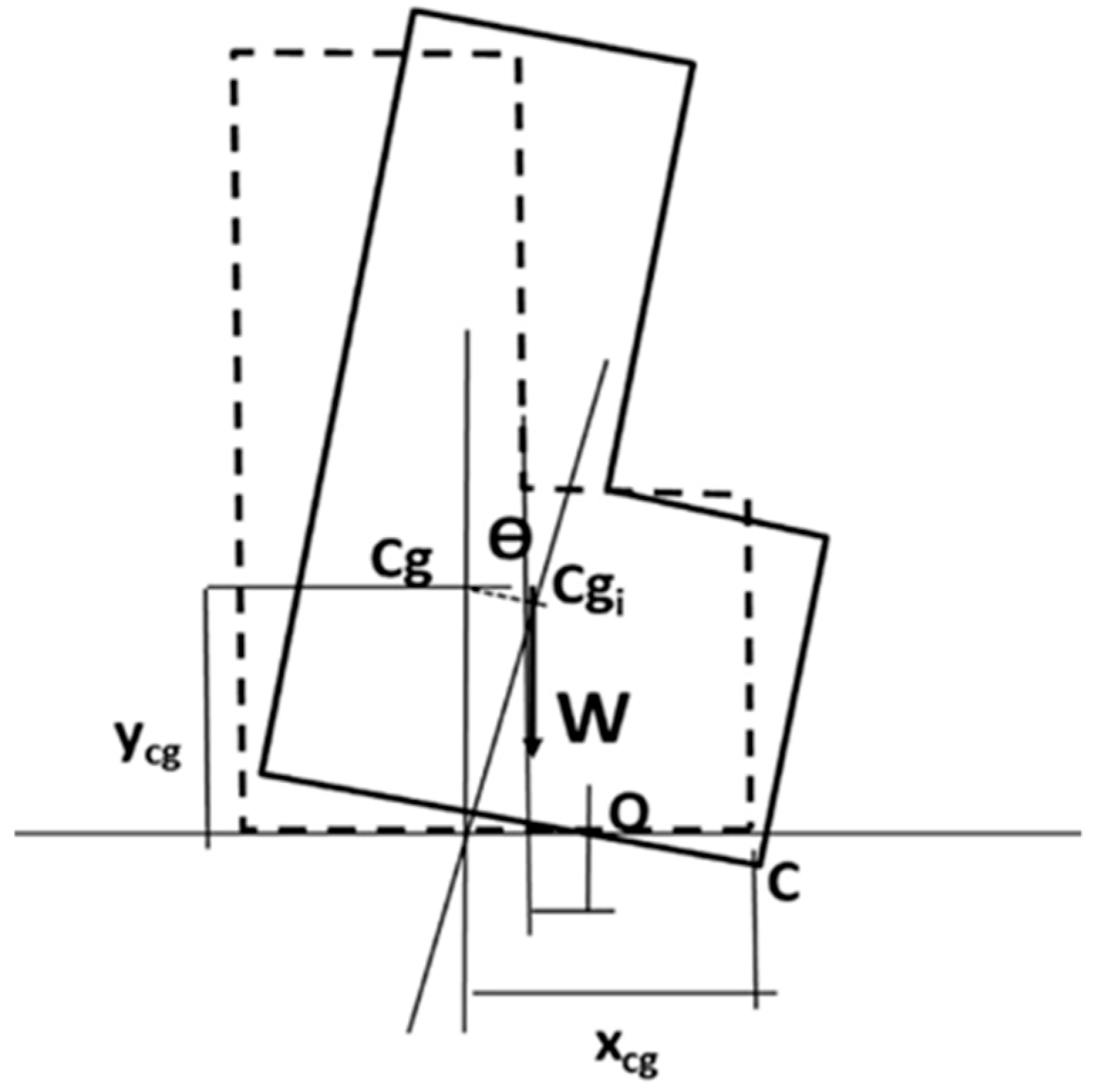
In addition, another damping of the turning movement is produced as a consequence of the stabilizing moment. This is generated as a consequence of the location of the centre of gravity of the crown wall with respect to the point of turning. If the projection is located towards the seaward side of point “O” (Figure A5), it is necessary to introduce it in the iterative process.

M_{stab} = W \times \bar{x_{CG}_{i} O_{i}} where, {\bar{x_{CG}_{i} O}}_{i} = {\bar{x_{CG}_{0} O}}_{i} - y_{CG} tg (θ_{i})

(A12)

The consequent damping in the turn is equal to a stabilizing turn:

θ_{i}^{estab} = \iint M_{{stab}_{i} dtdt} / I_{O}

(A13)

Therefore, adding this stabilizing turn as well as the net rotation obtained in Equation (A11) at the instant “i” of load application, the following total net rotation occurs (Equation (A14)):

θ_{i}_{net}^{total} = θ_{i}_{net} - θ_{i - 1}^{stab}

(A14)

Figure A5. Damping of the rotation as a result of the stabilizing moment.

Appendix A.2.3. Damping Corresponding to Movement

The same simplification done for the turn can be done for displacements, and the movement of the crown wall along the x-axis and the soil reaction due to its stiffness before its breakage could be estimated. However, in the case of movements, it is considered, according to Coulomb’s hypothesis [20], that the resistance of the soil to the movement is proportional to the normal force applied against the soil and independent of the velocity.

Appendix A.3. Simplified Model

Therefore, the system of differential equations and its resolution in the time domain are considerably simplified. The system of equations can be written in a simpler matrix form (Equation (A15)):

[\begin{matrix} m & {mr}_{CG} \\ {mr}_{CG} & I_{O} \end{matrix}] [\begin{matrix} \ddot{x} \\ \ddot{θ} \end{matrix}] + [\begin{matrix} 0 & 0 \\ 0 & k_{θ} \end{matrix}] [\begin{matrix} x \\ θ \end{matrix}] = [\begin{matrix} G_{Displ} \\ M_{O} \end{matrix}]

(A15)

where x—crown wall movement, ϴ—crown wall turn, m—crown wall mass, r_CG—distance of the centre of gravity of the crown wall to the turning point “O”, M_O—turning moment related to the point “O”, and I_O—inertial moment with respect to point “O”.

Furthermore,

k_{θ} = [({π EB}^{*}^{2}) / (4 (1 - ν^{2}))] (1 + 0.1 B^{*} / D)

, where B*—equivalent foundation breath, D—depth of non-deformable soil related to the crown wall foundation, E—Young’s modulus, and ν—Poisson coefficient. Finally,

G_{Displ} = (1 - p) [F_{x} - μ (W - F_{y})]

, where p—percentage of reduction of F_x as a function of the water mass that returns in the opposite direction of the movement and the reduced relative velocity of the wave and the moveable section compared to a fixed structure [20] (it is considered tp = 0, µ—friction coefficient, F_x—horizontal forces, F_y—vertical forces, W—m·g, and g—gravity.

According to this simplification, the transversal deformation of the soil is now introduced in the calculation, taking into account that until the slip condition is exceeded, there is no movement. So, this horizontal movement of the soil can be limited better by means of the following expression (Equation (A16)):

ε_{x} {_{%}}_{\max} = \max (q_{h} / G_{tang})

(A16)

where

q_{h} = F_{x} / B

is the horizontal shear pressure and G_tang is the tangent shear modulus.

The movement estimation presented with this simplification (Equation (A15)) is considered to be more precise than that presented by Burcharth et al. [21] (Equation (A17)) for the analysis of the movement of a caisson subjected to a horizontal force when introducing the effect of the turning movement of the crown wall:

F (t) = F_{x} (t) - (W - F_{y} (t)) μ_{t} = (m_{caisson} + m_{added}) \ddot{x}

(A17)

where W—weight of the caisson, m_caisson—mass of the caisson, and m_added—water mass that overtops the caisson and contributes to its stability.

The formula proposed by Burcharth et al. [21] (Equation (A17)) was checked against a numerical model of finite elements, in the case of a vertical caisson [22], underestimating the movements as a function of the permeability characteristics of the foundation, and in the case of crown walls [20], being on the safe side. However, it can be valid as an approximation if the movement of the core of the breakwater is not taken into account and we consider the relative movements to be absolute with respect to a specific point. This approach is useful for many of the usual problems in port engineering.

Appendix B. Elasto-Plastic Model of the Soil Proposed

The study was developed considering the hyperbolic elasto-plastic model of soil response proposed by Schanz et al. [10] and Kondner [11], considering the hysteresis of the materials, introducing a variable stress–strain relation according to the following expression (Equation (A18)):

E_{tang} = {dQ}_{H} / {d ε}_{y} = (1 / E_{0}) / [{(1 / E_{0} + ε_{a} / q_{a})}^{2}]

(A18)

where

Q_{H} = ε_{a} / (1 / E_{o} + ε_{a} / q_{a})

, E₀—initial Young’s modulus of elasticity, E_tang—tangent Young’s modulus for a specific deformation %ε_a, q_a—deviator in the asymptote of the hyperbola (difference between total vertical load and horizontal strain of the soil) and ε_a—vertical deformation of the soil (%).

The following adjustment parameters are proposed (Table A1):

Table A1. Adjustment parameters of the soil considered (initial Young module and Deviator).

Type of Soil	E₀ (MPa)	q_a (KN)
1	10	350
2	50	400
3	100	500
4	200	600
5	400	700

The analysis is presented in the following curves, with stress–strain relation and variation of the elasticity modulus as a function of deformation (Figure A6):

Figure A6. (A) Stress–strain relation and (B) Young’s modulus variation with deformation of the soil.

To analyze the failure of the system, it is proposed to consider as the admissible deformation of each material the value that corresponds to the application of 85% of the deviator in the asymptote (Table A2); e.g., approximately 5% of E₀.

Table A2. Admissible deformation definition.

E (MPa)	Deviator in the Asymtote (KN)	Admissible Deviator (KN)	%ε_y Admissible
10	350	280	19.8%
50	400	320	4.5%
100	500	400	2.8%
200	600	480	1.7%
400	700	560	1.0%

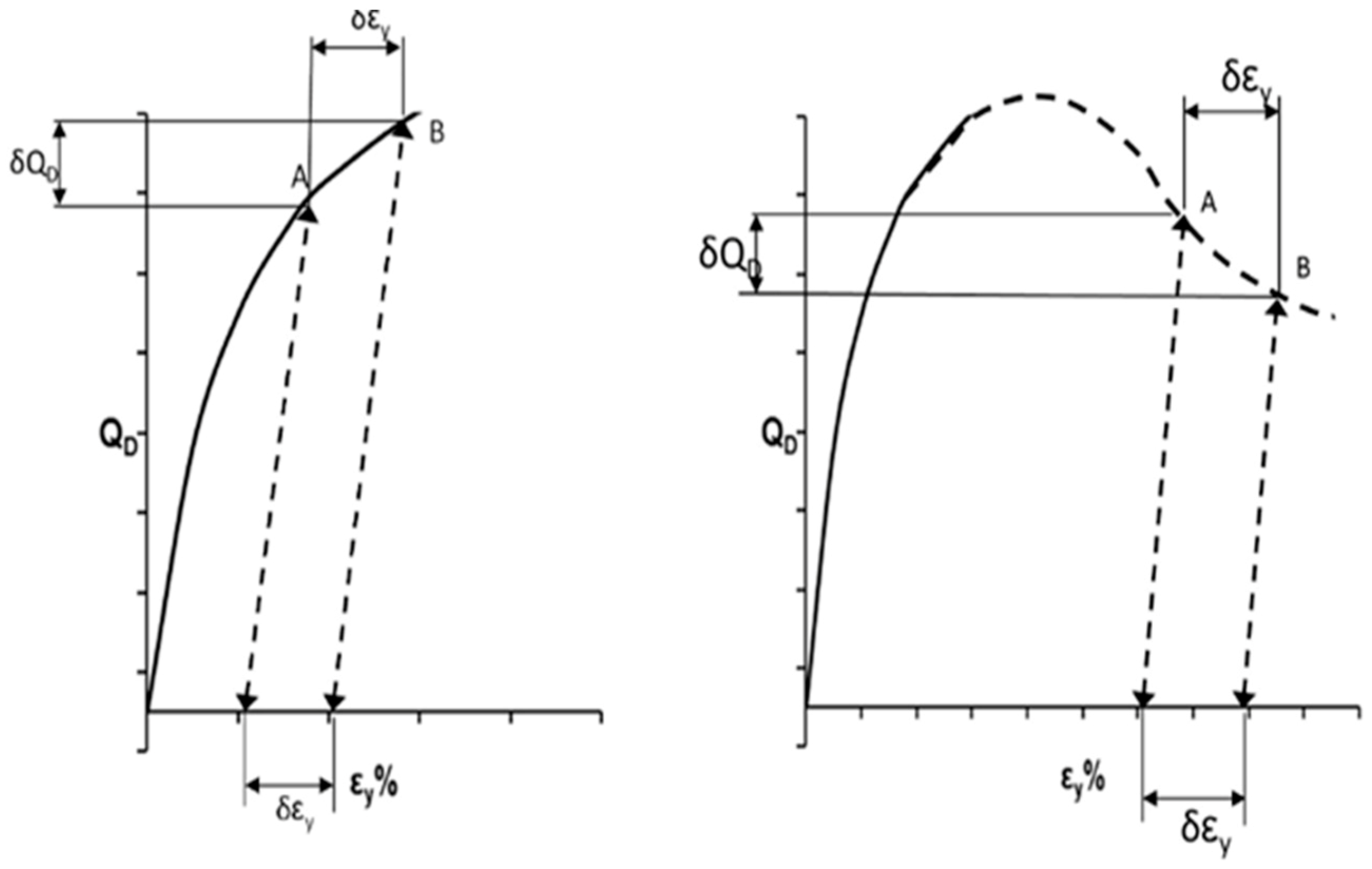
On the other hand, to take into account that the stiffness of the soil increases in the load reduction process, it is proposed to consider that during the recovery process, Young’s modulus increases up to E_rec = E₀ = 2E₅₀. Therefore, the stress–strain diagram considered in the loading–unloading process has the following form (Figure A7).

Figure A7. Stress–strain diagram of the loading–unloading process.

To consider the hysteresis of the materials, the model proposed by Atkinson [16] is applied. When the stress exceeds the yield point, residual deformations accumulate to the elastic deformations. Once the load has been reduced, according the stress–strain diagram of Figure A7, in a new cycle of reloading, the yield point moves upward in the stress–strain curve. It follows a process of hardening by deformation (Figure A8), up to the deformation that is considered as breakage, as suggested by Atkinson [16].

Figure A8. Process of hardening and softening produced by deformation, adapted from Atkinson [14].

References

US Army Corps of Engineers. Coastal Engineering Manual; US Army Corps of Engineers: Washington, DC, USA, 2002; Part 6, Chapter VI-5—Fundamentals of Design.
Pedersen, J. Wave Forces and Overtopping on Crown Walls of Rubble Mound Breakwaters: An Experimental Study; Aalborg University: Aalborg, Denmark, 1996; ISSN 0909-4296. [Google Scholar]
Kortenhaus, A.; Oumeraci, H. Clasification of wave loading on monolithic coastal structures. In Proceedings of the 26th Conference on Coastal Engineering, Copenhagen, Denmark, 22–26 June 1998; pp. 1–14. [Google Scholar] [CrossRef]
Cuomo, G.; Allsop, W.; Bruce, T.; Pearson, J. Breaking wave loads at vertical walls and breakwaters. Coast. Eng. 2010, 57, 424–439. [Google Scholar] [CrossRef]
Gomez-Barquín, G. Análisis Dinámico de un Dique de Abrigo Vertical, 1st ed.; Asociación Técnica de Puertos y Costas (Spanish Section of PIANC): Madrid, Spain, 1998. [Google Scholar]
Lamberti, A.; Martinelli, L.; de Groot, M.B. Dynamics. In Mast III/Proverbs, Volume IIb (Geotechnical Aspects); de Groot, M.B., Ed.; Technical University of Braunschweig: Braunschweig, Germany, 1999. [Google Scholar]
Plaxis. Plaxis 2D Scientific Manual; Delft University of Technology and Plaxis: Delft, The Netherlands, 2017. [Google Scholar]
Itasca. An Introduction to Flac 8 and a Guide To Its Practical Application in Geotechnical Engineering; Itasca: Minneapolis, MN, USA, 2015. [Google Scholar]
Kvalstad, T. Degradation and residual pore pressures. In Mast III/Proverbs, Volume IIb (Geotechnical Aspects); de Groot, M.B., Ed.; Technical University of Braunschweig: Braunschweig, Germany, 1999. [Google Scholar]
Schanz, T.; Vermeer, A.; Bonnier, P. The Hardening Soil Model: Formulation and Verification. In Proceedings of the Beyond 2000 Computational Geotechnics 10 Years PLAXIS, Amsterdam, The Netherlands, March 1999. [Google Scholar]
Kondner, R.L. Hyperbolic stress-strain response: Cohesive soils. J. Soil Mech. Found. Div. 1963, 89, 115–144. [Google Scholar] [CrossRef]
CEDEX. Ensayo en Modelo Físico 2D a Gran esCala Sobre la Sección Tipo del Dique del Nuevo Puerto Exterior de La Coruña en Punta Langosteira; CEDEX: Madrid, Spain, 2005. [Google Scholar]
Soriano, A. Movimientos del Espaldón Durante un Temporal; Dique de Langosteira, Autoridad Portuaria de A Coruña: A Coruña, Spain, 2016. (In Spanish) [Google Scholar]
CEDEX. Informe de Laboratorio para UTE Galería Langosteira, Proyecto Constructivo de galería para protección de tuberías en el dique de las nuevas instalaciones portuarias en Punta Langosteir; CEDEX: Madrid, Spain, 2016. [Google Scholar]
Hansen, J.B. A Revised and Extended Formula for Bearing Capacity; Bulletin No. 28; Danish Geotechnical Institute: Copenhagen, Denmark, 1970; pp. 5–11. [Google Scholar]
Atkinson, J. The Mechanics of Soils and Foundations, 2nd ed.; Taylor & Francis: Abingdon, UK, 2007; 475p, ISBN 9780415362566. [Google Scholar]
Jimenez Salas, J.A.; de Justo, J.L.; Serrano, A.A. Geotecnia y Cimientos II. Mecánica del suelo y de las Rocas, 2nd ed.; Rueda: Madrid, Spain, 1981; p. 1188. ISBN 84-7207-021-2. [Google Scholar]
Recomendaciones Geotécnicas para Obras Marítimas y Portuarias, 1st ed.; ROM 0.5.05; Puertos del Estado: Madrid, Spain, 2005; 546p, ISBN 84-88975-52-X.
Gazetas, G. Analysis of machine foundation vibrations: State of the art. Int. J. Soil Dyn. Earthq. Eng. 1983, 2, 2–42. [Google Scholar] [CrossRef]
Nørgaard, J.Q.H.; Andersen, L.V.; Andersen, T.L.; Burcharth, H.F. Displacement of monolithic rubble-mound breakwater crown-walls. In Proceedings of the 33rd International Conference on Coastal Engineering, Santander, Spain, 29–30 June 2012; Volume 2, pp. 966–981. [Google Scholar]
Burcharth, H.F.; Andersen, L.; Andersen, T.L. Analyses of stability of caisson breakwaters on rubble foundation exposed to impulsive loads. In Coastal Engineering 2008; World Scientific Publishing Company: Singapore, 2009; pp. 3606–3618. [Google Scholar] [CrossRef]
Andersen, L.; Burcharth, H.F.; Lykke Andersen, T. Validity of Simplified Analysis of Stability of Caisson Breakwaters on Rubble Foundation Exposed to Impulsive Loads. In Proceedings of the 32nd International Conference on Coastal Engineering, Shanghai, China, 30 June–5 July 2010; Volume 46, pp. 1–14. [Google Scholar] [CrossRef]

Figure 1. Breakwater modes of failure (adapted from Pedersen [2]).

Figure 2. Cross section of the main breakwater of the outer port of Punta Langosteira (A Coruña, Spain).

Figure 3. Load state A, used for crown wall design (Wave height Hs (m) = 15.1; Peak period Tp (s) = 20), [11].

Figure 4. Load state B.

Figure 5. Load state C.

Figure 6. Shape of the load state A in the time domain: (A) horizontal force (F_x); (B) overturning moment (M).

Figure 7. Shape of the load states B and C in the time domain: (A) horizontal force (Fx); (B) overturning moment (M).

Figure 8. (A) Movement on the top of the crown wall; (B) maximum vertical deformation of the foundation.

Figure 9. Expected movement on the top of the foundation: E (MPa) = 10; 2 load cycles.

Figure 10. Sinusoidal force. (A) Movement on the top of the crown wall; (B) angular velocity, related to the overturning moment. E (MPa) = 10; 2 load cycles.

Figure 11. Impulsive 1. (A) Movement on the top of the crown wall; (B) angular velocity, related to overturning moment. E (MPa) = 10; 2 load cycles.

Figure 12. (A) Movement on the top of the crown wall; (B) maximum vertical deformation of the foundation.

Figure 13. (A) Residual movement on the top of the crown wall; (B) residual vertical deformation.

Figure 14. (A) Movements on the top of the crown wall; (B) stress–strain graph showing the relationship between the load deviator and vertical deformation produced in the first and second cycles of loading.

Figure 15. Tip factor influence: (A) shape of the signals; (B) movements on the top of the foundation. 2 cycles.

Figure 16. Rise time influence: (A) shape of the signals; (B) movements on the top of the foundation.

Figure 17. Crown wall displacement as a function of Sliding Safety Coefficient (SSC) and Young’s modulus of the soil, assuming elastic soil, for the 4 different theoretical signals: (A) Permanent; (B) Sinusoidal; (C) Impulsive 1; (D) Impulsive 2.

Figure 18. Displacement of the upper part of the crown wall in the breakwater of A Garda, Spain (2017).

Figure 19. Wall sliding as a function of SSC and the signal shape, assuming elastic soil. (A) E (MPa) = 10; (B); E (MPa) = 100; (C) E (MPa) = 27,000.

Figure 20. Maximum deformation as a function of the bearing capacity safety coefficient (BCSC) and Young’s modulus of the soil, assuming elastic soil. (A) Permanent; (B) Sinusoidal; (C) Impulsive 1; (D) Impulsive 2.

Figure 21. Wall rotation as a function of Overturning Safety coefficient (OSC) and Young’s modulus, assuming elastic soil. (A) Permanent; (B) Sinusoidal; (C) Impulsive 1; (D) Impulsive 2.

Figure 22. Crown wall rotation as a function of OSC and the shape of the signal, assuming elastic soil (A) E (MPa) = 10; (B) E (MPa) = 100; (C); E (MPa) = 27,000.

Figure 23. Soil deformation as a function of Bearing Capacity Safety Coefficient (BCSC) and Young’s modulus. Permanent: (A) elastic soil; (B) elasto-plastic soil. Sinusoidal: (C) elastic soil; (D) elasto-plastic soil. Impulsive 1: (E) elastic soil; (F) elasto-plastic soil. Impulsive 2: (G) elastic soil; (H) elasto-plastic soil.

Table 1. Safety coefficients obtained for load state A.

Mode of Failure	Safety Coefficient	Verification
Sliding safety coefficient (SSC)	1.93
Rigid overturning safety coefficient (OSC)	4.61
Bearing capacity safety coefficient (BCSC)	6.24	Brinch-Jansen [15]

Table 2. Safety coefficients obtained for load state B.

F_x (KN) (Horizontal Force)	1000	1200	1400	1600	1800	2000	2200
Sliding Safety Coefficient (SSC)	1.62	1.35	1.16	1.01	0.90	0.81	0.74
Overturning Safety Coefficient (OSC)	3.27	2.55	2.18	1.91	1.70	1.53	1.39
Bearing Capacity Safety Coefficient (BCSC) [15]	4.34	2.86	1.83	1.14	0.69	0.40	0.22

Table 3. Coefficients obtained for load state C.

M (KNm) (Overturning Moment)	4800	7200	9600	10,800	12,000	14,400	15,600	16,800	19,200
Sliding Safety Coefficient (SSC)	1.35	1.35	1.35	1.47	1.35	1.35	1.35	1.35	1.35
Overturning Safety Coefficient (OSC)	3.31	2.21	1.66	1.35	1.33	1.10	1.02	0.95	0.83
Bearing Capacity Safety Coefficient (BCSC) [15]	3.44	2.49	1.66	1.29	0.96	0.35	0.07	0.01	0

Table 4. Results obtained with the simplified model and with FLAC2D 7.0 code, comparison without considering transverse deformation of the soil.

E (MPa) Considering the Worst Values for the Core	Poisson Coefficient	Shape of the Load’s Signal	Simplified Model (Elastic)		FLAC2D 7.0 (Net Movements)
E (MPa) Considering the Worst Values for the Core	Poisson Coefficient	Shape of the Load’s Signal	Top Displacement (m)	ε_y%	Top Displacement (m)	ε_y%
10	0.30	1	0.27	1.8	0.30	2.0
30	0.30	1	0.08	0.5	0.07	0.5

Table 5. Results obtained with the simplified model and with FLAC2D 7.0 code, comparison considering transverse deformation of the soil.

E (MPa) Considering the Worst Values for the Core	Poisson Coefficient	Shape of the Load’s Signal	Simplified Model (Elastic)			FLAC2D 7.0 (Total Movements)
E (MPa) Considering the Worst Values for the Core	Poisson Coefficient	Shape of the Load’s Signal	Top Displacement (m)	ε_y%	ε_x%	Top Displacement (m)	ε_y%	ε_x%
10	0.30	1	0.49	1.8	2.2	0.46	2.0	1.6
30	0.30	1	0.16	0.6	0.7	0.13	0.5	0.6

Where ε_x%— soil deformation in X-axis; ε_y%—soil deformation in Y-axis.

Table 6. Crown wall sliding in simulations under load state B.

Sliding Failure (m of Displacement, 10 Cycles of Load)
Sliding Safety Coefficient		1.35	1.16	1.01	0.90	0.81	0.74	1.35	1.16	1.01	0.90	0.81	0.74
Young’s Modulus	Signal	Elastic Soil						Elasto-Plastic Soil
E = 10 MPa	Permanent	-	-	-	9.9	14.0	18.3	-	-	-	9.9	14.0	18.3
	Sinusoidal	-	-	-	-	-	2.0	-	-	-	-	-	2.0
	Impulsive 1	-	-	-	-	-	0.2	-	-	-	-	-	0.2
	Impulsive 2	-	-	-	-	-	0.1	-	-	-	-	-	0.1
E = 50 MPa	Permanent	-	-	-	10.4	14.5	18.7	-	-	-	10.4	14.5	18.7
	Sinusoidal	-	-	-	1.1	2.2	3.3	-	-	-	1.1	2.2	3.3
	Impulsive 1	-	-	-	-	-	2.2	-	-	-	-	-	2.2
	Impulsive 2	-	-	-	-	-	0.2	-	-	-	-	-	0.2
E = 100 MPa	Permanent	-	-	-	10.4	14.6	18.7	-	-	-	10.4	14.5	18.7
	Sinusoidal	-	-	-	1.3	2.3	3.4	-	-	-	1.3	2.3	3.4
	Impulsive 1	-	-	-	-	1.4	2.5	-	-	-	-	1.4	2.5
	Impulsive 2	-	-	-	-	0.2	0.4	-	-	-	-	0.2	0.4
E = 200 MPa	Permanent	-	-	-	10.4	14.6	18.7	-	-	-	10.4	14.6	18.7
	Sinusoidal	-	-	-	1.4	2.4	3.5	-	-	-	1.4	2.4	3.5
	Impulsive 1	-	-	-	-	1.5	2.6	-	-	-	-	1.5	2.6
	Impulsive 2	-	-	-	-	0.3	0.5	-	-	-	-	0.3	0.5
E = 400 MPa	Permanent	-	-	-	10.4	14.6	18.7	-	-	-	10.4	14.6	18.7
	Sinusoidal	-	-	-	1.5	2.5	3.5	-	-	-	1.5	2.5	3.5
	Impulsive 1	-	-	-	0.6	1.6	2.6	-	-	-	0.5	1.5	2.6
	Impulsive 2	-	-	-	0.1	0.3	0.5	-	-	-	0.1	0.3	0.5
E = 27,000 MPa	Permanent	-	-	-	10.4	14.6	18.7
	Sinusoidal	-	-	-	1.5	2.5	3.6
	Impulsive 1	-	-	-	0.5	1.5	2.7
	Impulsive 2	-	-	-	0.2	0.3	0.5

Table 7. Vertical deformation in simulations under load state B.

Sliding Failure (% of Vertical Deformation)
Sliding Safety Coefficient		1.35	1.16	1.01	0.90	0.81	0.74	1.35	1.16	1.01	0.90	0.81	0.74
Young’s Modulus	Signal	Elastic Soil						Elasto-Plastic Soil
E = 10 MPa	Permanent	4.1%	5.9%	8.9%	8.4%	7.8%	7.8%	6.5%	9.7%	15.6%	14.5%	13.4%	13.3%
	Sinusoidal	3.5%	4.5%	5.8%	6.4%	6.6%	5.4%	5.4%	7.3%	9.6%	10.9%	11.1%	8.9%
	Impulsive 1	2.6%	3.4%	4.3%	5.3%	6.4%	7.2%	3.7%	5.0%	6.6%	8.5%	10.6%	12.1%
	Impulsive 2	1.5%	1.8%	2.1%	2.5%	3.0%	3.5%	2.6%	3.1%	3.7%	4.5%	5.4%	6.4%
E = 50 MPa	Permanent	0.7%	1.1%	1.5%	1.4%	1.3%	1.1%	1.3%	1.9%	2.8%	2.6%	2.2%	1.9%
	Sinusoidal	0.8%	1.1%	1.6%	1.6%	1.5%	1.4%	1.4%	2.0%	2.9%	2.9%	2.7%	2.6%
	Impulsive 1	0.7%	0.9%	1.2%	1.4%	1.6%	1.4%	1.0%	1.4%	1.9%	2.2%	2.6%	2.4%
	Impulsive 2	0.5%	0.7%	0.9%	1.1%	1.2%	1.1%	1.1%	1.4%	1.8%	2.2%	2.3%	2.1%
E = 100 MPa	Permanent	0.3%	0.5%	0.7%	0.7%	0.6%	0.5%	0.6%	0.9%	1.3%	1.3%	1.0%	0.9%
	Sinusoidal	0.3%	0.5%	0.7%	0.7%	0.7%	0.7%	0.7%	1.0%	1.5%	1.5%	1.4%	1.4%
	Impulsive 1	0.4%	0.5%	0.7%	0.8%	0.7%	0.7%	0.6%	0.8%	1.1%	1.4%	1.1%	1.1%
	Impulsive 2	0.3%	0.4%	0.5%	0.6%	0.6%	0.6%	0.7%	0.9%	1.2%	1.4%	1.2%	1.2%
E = 200 MPa	Permanent	0.1%	0.2%	0.3%	0.3%	0.3%	0.2%	0.3%	0.4%	0.7%	0.6%	0.5%	0.4%
	Sinusoidal	0.1%	0.2%	0.3%	0.3%	0.3%	0.3%	0.3%	0.5%	0.7%	0.7%	0.7%	0.7%
	Impulsive 1	0.2%	0.3%	0.4%	0.5%	0.4%	0.4%	0.3%	0.4%	0.6%	0.8%	0.6%	0.6%
	Impulsive 2	0.1%	0.2%	0.3%	0.3%	0.3%	0.3%	0.4%	0.5%	0.7%	0.8%	0.7%	0.7%
E = 400 MPa	Permanent	0.1%	0.1%	0.1%	0.1%	0.1%	0.1%	0.2%	0.2%	0.3%	0.3%	0.3%	0.2%
	Sinusoidal	0.1%	0.1%	0.1%	0.1%	0.1%	0.2%	0.2%	0.2%	0.4%	0.4%	0.4%	0.4%
	Impulsive 1	0.1%	0.2%	0.2%	0.2%	0.2%	0.1%	0.2%	0.2%	0.3%	0.3%	0.3%	0.3%
	Impulsive 2	0.1%	0.1%	0.1%	0.1%	0.1%	0.1%	0.2%	0.3%	0.4%	0.4%	0.4%	0.4%
E = 27,000 MPa	Permanent	0.0%	0.0%	0.0%	0.0%	0.0%	0.0%
	Sinusoidal	0.0%	0.0%	0.0%	0.0%	0.0%	0.0%
	Impulsive 1	0.0%	0.0%	0.0%	0.0%	0.0%	0.0%
	Impulsive 2	0.0%	0.0%	0.0%	0.0%	0.0%	0.0%

Table 8. Modes of failure in the simulations carried out under load state B and safety coefficients obtained at failure.

Failures Produced in Simulations under Load State B
Young’s Modulus	Signal	Elastic Soil			Elasto-Plastic Soil
		Safety Coefficient at the Time of Failure		Mode of Failure	Safety Coefficient at the Time of Failure		Mode of Failure
		SSC	BCSC	Mode of Failure	SSC	BCSC	Mode of Failure
E = 10 MPa	Permanent	1.01	1.14	SLIDING	1.01	1.14	SLIDING
	Sinusoidal	0.81	0.40	SLIDING	0.81	0.40	SLIDING
	Impulsive 1	0.81	0.40	SLIDING	0.81	0.40	SLIDING
	Impulsive 2	0.81	0.40	SLIDING	0.81	0.40	SLIDING
E = 50 MPa	Permanent	1.01	1.14	SLIDING	1.01	1.14	SLIDING
	Sinusoidal	1.01	1.14	SLIDING	1.01	1.14	SLIDING
	Impulsive 1	0.81	0.40	SLIDING	0.81	0.40	SLIDING
	Impulsive 2	0.81	0.40	SLIDING	0.81	0.40	SLIDING
E = 100 MPa	Permanent	1.01	1.14	SLIDING	1.01	1.14	SLIDING
	Sinusoidal	1.01	1.14	SLIDING	1.01	1.14	SLIDING
	Impulsive 1	0.90	0.69	SLIDING	0.90	0.69	SLIDING
	Impulsive 2	0.90	0.69	SLIDING	0.90	0.69	SLIDING
E = 200 MPa	Permanent	1.01	1.14	SLIDING	1.01	1.14	SLIDING
	Sinusoidal	1.01	1.14	SLIDING	1.01	1.14	SLIDING
	Impulsive 1	0.90	0.69	SLIDING	0.90	0.69	SLIDING
	Impulsive 2	0.90	0.69	SLIDING	0.90	0.69	SLIDING
E = 400 MPa	Permanent	1.01	1.14	SLIDING	1.01	1.14	SLIDING
	Sinusoidal	1.01	1.14	SLIDING	1.01	1.14	SLIDING
	Impulsive 1	1.01	1.14	SLIDING	1.01	1.14	SLIDING
	Impulsive 2	1.01	1.14	SLIDING	1.01	1.14	SLIDING
E = 27,000 MPa	Permanent	1.01		SLIDING
	Sinusoidal	1.01		SLIDING
	Impulsive 1	1.01		SLIDING
	Impulsive 2	1.01		SLIDING

Table 9. Crown wall turning in simulations under load state C. [The simulations with failure of the structure are highlighted in dark gray (failure due to rigid overturning) and in light gray (failure due to bearing capacity of the foundation)].

Bearing Capacity and Overturning Failure (Rotation in Degrees)
Bearing Capacity Safety Coefficient		2.49	1.66	1.29	0.96	0.35	0.07	0.01	2.49	1.66	1.29	0.96	0.35	0.07	0.00
Overturning Safety Coefficient		2.21	1.66	1.47	1.33	1.10	1.02	0.95	2.21	1.66	1.47	1.33	1.10	1.02	0.95
Young’s Modulus	Signal	Elastic Soil							Elasto-Plastic Soil
10 MPa	Permanent	3.3	7.4	11.7	23.8	90.0	90.0	90.0	5.4	13.4	21.9	46.1	90.0	90.0	90.0
	Sinusoidal	2.5	4.0	4.5	4.9	5.3	5.3	5.3	4.1	6.8	7.8	8.5	9.3	9.3	9.4
	Impulsive 1	1.8	3.1	4.0	4.5	5.2	5.3	5.4	2.8	5.2	6.9	7.8	9.0	9.3	9.4
	Impulsive 2	1.0	1.5	1.9	2.2	3.1	3.6	4.1	1.8	2.7	3.3	4.1	5.8	6.7	7.8
50 MPa	Permanent	0.6	1.2	1.8	3.1	35.9	90.0	90.0	1.1	2.3	3.5	5.9	73.5	90.0	90.0
	Sinusoidal	0.6	1.2	1.6	2.0	3.0	3.3	3.5	1.1	2.3	3.0	4.0	6.0	6.7	7.2
	Impulsive 1	0.4	0.8	0.9	1.1	1.9	2.4	3.0	0.8	1.4	1.7	2.1	3.7	4.8	6.0
	Impulsive 2	0.4	0.6	0.7	0.8	1.0	1.0	1.0	0.8	1.3	1.5	1.7	2.0	2.1	2.1
100 MPa	Permanent	0.3	0.6	0.9	1.4	10.6	90.0	90.0	0.5	1.1	1.7	2.8	21.9	90.0	90.0
	Sinusoidal	0.3	0.6	0.8	1.1	2.1	2.5	2.8	0.6	1.2	1.7	2.4	4.6	5.5	6.3
	Impulsive 1	0.2	0.4	0.5	0.6	0.9	1.2	1.8	0.5	0.8	1.0	1.3	1.9	2.7	3.9
	Impulsive 2	0.2	0.4	0.5	0.5	0.7	0.7	0.8	0.5	0.9	1.0	1.2	1.5	1.6	1.7
200 MPa	Permanent	0.1	0.3	0.4	0.7	4.4	90.0	90.0	0.2	0.5	0.8	1.4	9.4	90.0	90.0
	Sinusoidal	0.1	0.3	0.4	0.6	1.4	1.8	2.2	0.3	0.6	0.9	1.4	3.3	4.5	5.4
	Impulsive 1	0.1	0.2	0.3	0.3	0.5	0.6	0.9	0.2	0.5	0.6	0.8	1.3	1.5	2.1
	Impulsive 2	0.1	0.2	0.2	0.3	0.4	0.5	0.5	0.3	0.5	0.6	0.8	1.1	1.2	1.4
400 MPa	Permanent	0.1	0.1	0.2	0.3	1.9	90.0	90.0	0.1	0.3	0.4	0.7	4.5	90.0	90.0
	Sinusoidal	0.0	0.1	0.2	0.2	0.8	1.2	1.5	0.1	0.3	0.4	0.7	2.4	3.7	4.8
	Impulsive 1	0.0	0.1	0.1	0.2	0.3	0.4	0.5	0.1	0.3	0.4	0.5	0.9	1.1	1.4
	Impulsive 2	0.0	0.1	0.1	0.2	0.3	0.3	0.4	0.2	0.3	0.4	0.5	0.8	0.9	1.1
27,000 MPa	Permanent	0.0	0.0	0.0	0.0	0.0	0.3	90.0
	Sinusoidal	0.0	0.0	0.0	0.0	0.0	0.0	0.1
	Impulsive 1	0.0	0.0	0.0	0.0	0.0	0.0	0.0
	Impulsive 2	0.0	0.0	0.0	0.0	0.0	0.0	0.0

Table 10. Mode of failure in simulations under load state C and safety coefficients obtained at the time of failure of the crown wall.

Failure Produced in Simulations under Load State C
Young’s Modulus	Signal	Maximum Acceptable Deformation	Elastic Soil			Elasto-Plastic Soil
			Safety Coefficient at the Time of Failure		Mode of Failure	Safety Coefficient at the Time of Failure		Mode of Failure
			BCSC	OSC	Mode of Failure	BCSC	OSC	Mode of Failure
E = 10 MPa	Permanent	19.8%	1.32	1.49	bearing capacity	1.88	1.80	bearing capacity
	Sinusoidal		no	no	no	no	no	no
	Impulsive 1		no	no	no	no	no	no
	Impulsive 2		no	no	no	no	no	no
E = 50 MPa	Permanent	4.5%	1.09	1.38	bearing capacity	1.58	1.62	bearing capacity
	Sinusoidal		0.59	1.19	bearing capacity	1.51	1.58	bearing capacity
	Impulsive 1		0.05	1.00	bearing capacity	0.79	1.26	bearing capacity
	Impulsive 2		no	no	no	0.00	0.83	bearing capacity
E = 100 MPa	Permanent	2.8%	0.95	1.32	bearing capacity	1.36	1.50	bearing capacity
	Sinusoidal		0.66	1.22	bearing capacity	1.36	1.51	bearing capacity
	Impulsive 1		0.03	0.97	bearing capacity	0.61	1.20	bearing capacity
	Impulsive 2		no	no	no	0.09	1.03	bearing capacity
E = 200 MPa	Permanent	1.7%	0.91	1.31	bearing capacity	1.20	1.43	bearing capacity
	Sinusoidal		0.64	1.21	bearing capacity	1.22	1.44	bearing capacity
	Impulsive 1		0.01	0.95	bearing capacity	0.73	1.24	bearing capacity
	Impulsive 2		no	no	no	0.58	1.17	bearing capacity
E = 400 MPa	Permanent	1.0%	0.85	1.29	bearing capacity	1.09	1.38	bearing capacity
	Sinusoidal		0.59	1.19	bearing capacity	1.14	1.40	bearing capacity
	Impulsive 1		0.01	0.84	bearing capacity	0.84	1.25	bearing capacity
	Impulsive 2		no	no	no	0.79	1.24	bearing capacity
E = 27,000 MPa	Permanent			1.00	overturning
	Sinusoidal			no	no
	Impulsive 1			no	no
	Impulsive 2			no	no

© 2019 by the authors. Licensee MDPI, Basel, Switzerland. This article is an open access article distributed under the terms and conditions of the Creative Commons Attribution (CC BY) license (http://creativecommons.org/licenses/by/4.0/).

Share and Cite

MDPI and ACS Style

Maciñeira, E.; Peña, E.; Sande, J.; Figuero, A. Dynamic Calculation of Breakwater Crown Walls under Wave Action: Influence of Soil Mechanics and Shape of the Loading State. Water 2019, 11, 1149. https://doi.org/10.3390/w11061149

AMA Style

Maciñeira E, Peña E, Sande J, Figuero A. Dynamic Calculation of Breakwater Crown Walls under Wave Action: Influence of Soil Mechanics and Shape of the Loading State. Water. 2019; 11(6):1149. https://doi.org/10.3390/w11061149

Chicago/Turabian Style

Maciñeira, Enrique, Enrique Peña, José Sande, and Andrés Figuero. 2019. "Dynamic Calculation of Breakwater Crown Walls under Wave Action: Influence of Soil Mechanics and Shape of the Loading State" Water 11, no. 6: 1149. https://doi.org/10.3390/w11061149

Note that from the first issue of 2016, this journal uses article numbers instead of page numbers. See further details here.

Article Menu

Dynamic Calculation of Breakwater Crown Walls under Wave Action: Influence of Soil Mechanics and Shape of the Loading State

Abstract

1. Introduction

2. Proposed Simplified Model

3. Case Study: Breakwater of Punta Langosteira, Spain

3.1. Breakwater and Crown Wall Description

3.2. Soil Mechanics Characteristics

3.3. Loading States

3.4. Shape of the Loading State Signal in the Time Domain

4. Results Obtained with the Simplified Model Proposed

4.1. Load State A

4.1.1. Elastic Soil

4.1.2. Elasto-Plastic Soil

4.1.3. Comparison with FLAC2D 7.0 Code

4.1.4. Influence of Tip Factor and Rise Time in the Church-Roof Signals

4.2. Load State B

4.3. Load State C

5. Conclusions

Author Contributions

Funding

Acknowledgments

Conflicts of Interest

Appendix A. Simplified Problem Approach

Appendix A.1. Soil Stiffness

Appendix A.1.1. Stiffness against Turning

Appendix A.1.2. Stiffness against Movement

Appendix A.2. Consideration of the Damping of the Movement

Appendix A.2.1. Damping Corresponding to the Turn

Appendix A.2.2. Inertial Damping

Appendix A.2.3. Damping Corresponding to Movement

Appendix A.3. Simplified Model

Appendix B. Elasto-Plastic Model of the Soil Proposed

References

Share and Cite

Article Metrics

Article Access Statistics

Further Information

Guidelines

MDPI Initiatives

Follow MDPI