The Implementation of a Hybrid Model for Hilly Sub-Watershed Prioritization Using Morphometric Variables: Case Study in India

 ,
, 

 ,
,  and
and 
Abstract
:1. Introduction
2. Materials and Methods
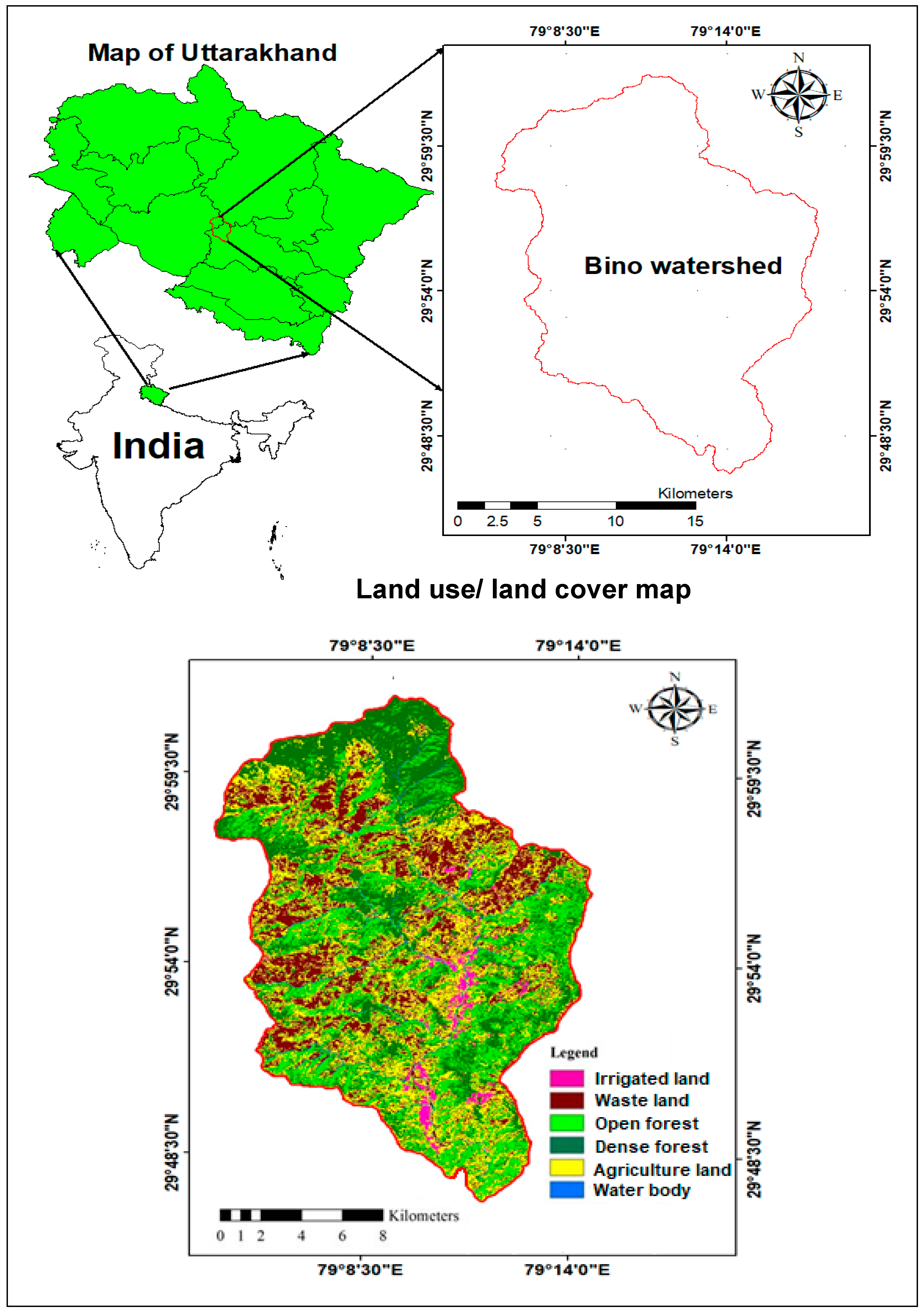
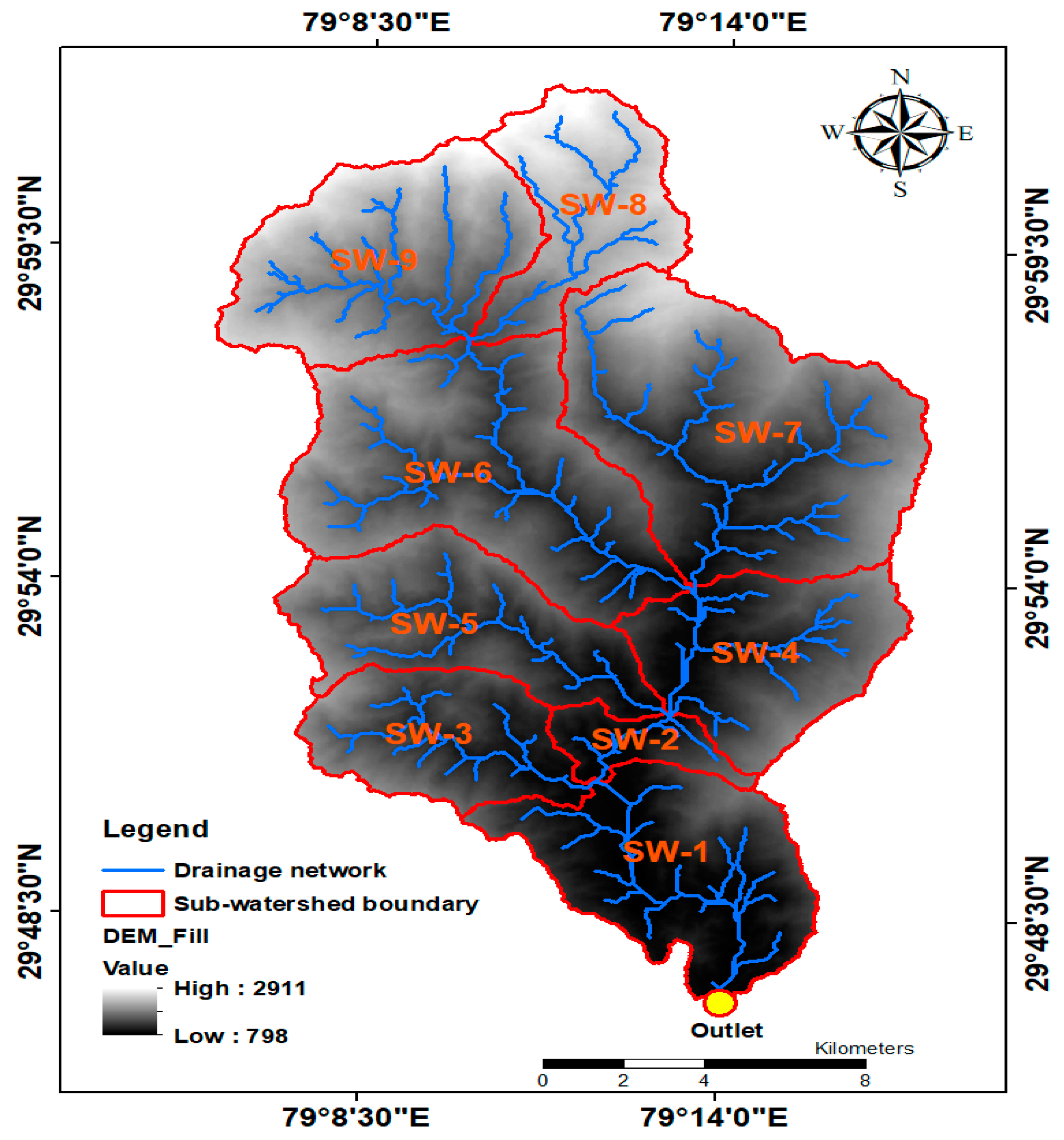
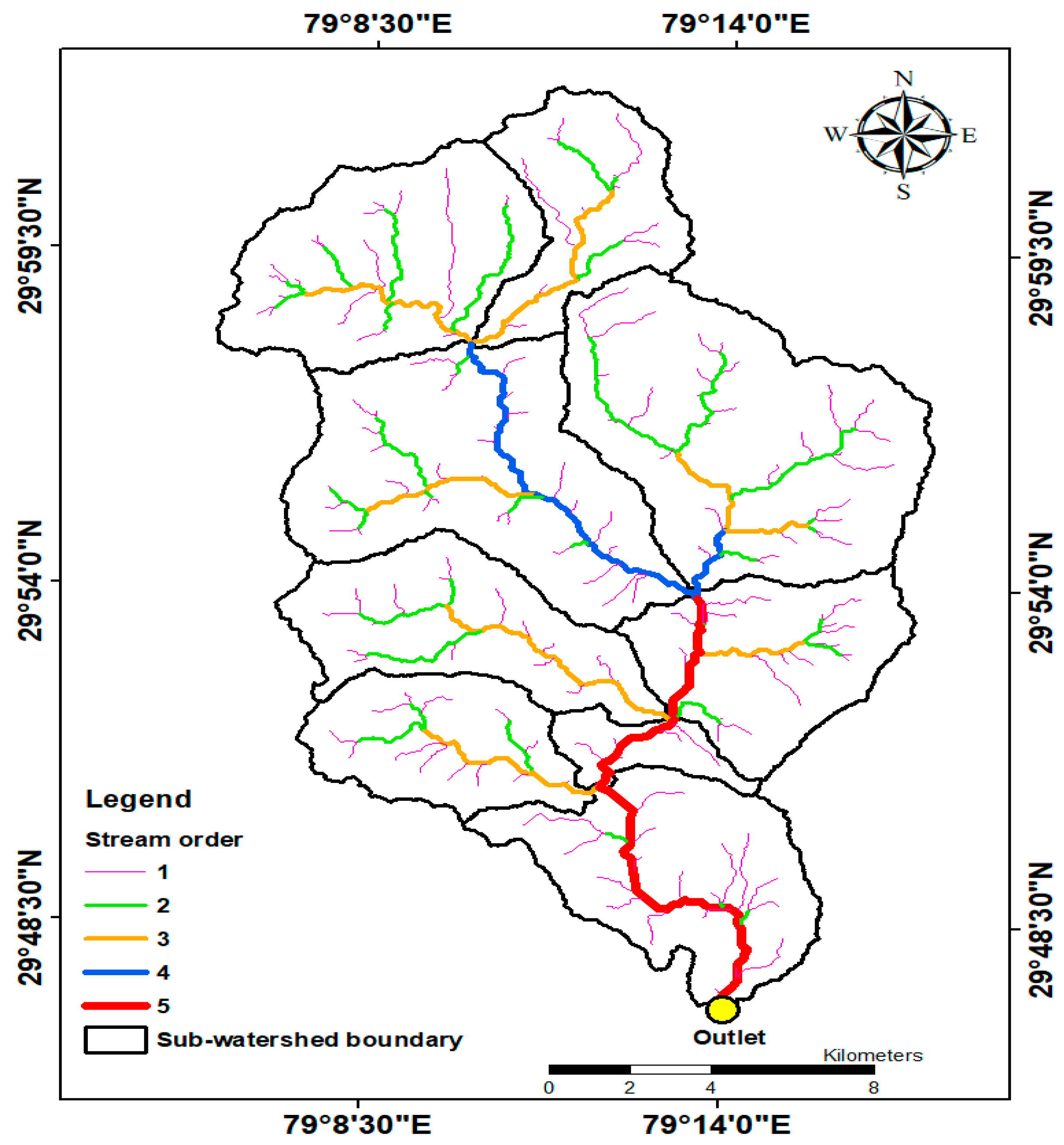
2.1. Case Study and Data Collection
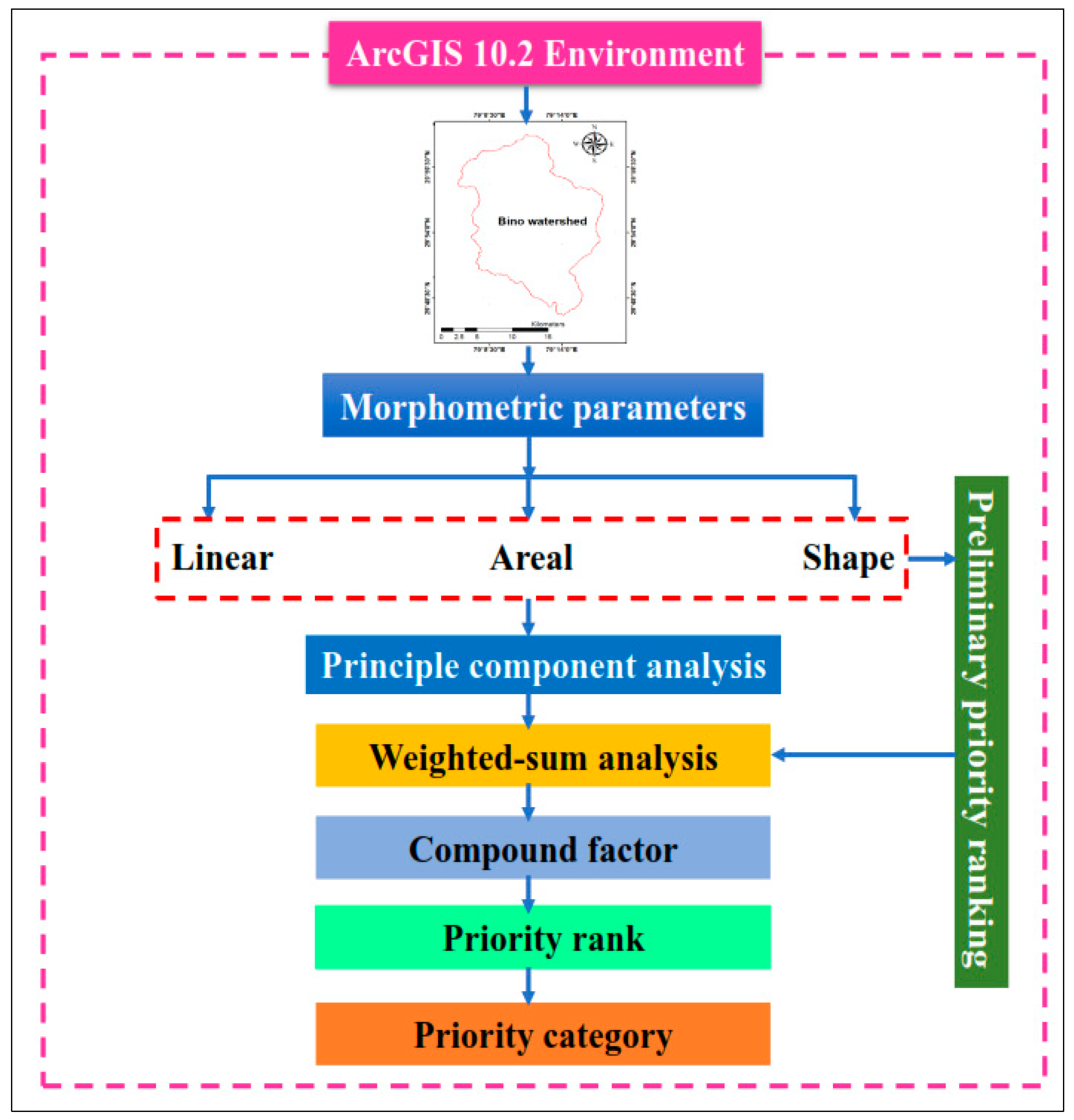
2.2. Morphometric Analysis and Assign Preliminary Priority Rank to the SWs
2.3. Principal Component Analysis and Weighted-Sum Approach
2.3.1. Principal Component Analysis
2.3.2. Weighted-Sum Approach
3. Application Results and Analysis
3.1. Principal Component Analysis of Morphometric Variables
3.2. Weighted-Sum Analysis of Significant Morphometric Variables
3.3. Prioritization of SW Using PCWSA
4. Discussion
5. Conclusions
Author Contributions
Conflicts of Interest
References
- Aher, P.; Adinarayana, J.; Gorantiwar, S. Quantification of morphometric characterization and prioritization for management planning in semi-arid tropics of India: A remote sensing and GIS approach. J. Hydrol. 2014, 511, 850–860. [Google Scholar] [CrossRef]
- Youssef, A.M.; Pradhan, B.; Hassan, A.M. Flash flood risk estimation along the St. Katherine road, southern Sinai, Egypt using GIS based morphometry and satellite imagery. Environ. Earth Sci. 2011, 62, 611–623. [Google Scholar] [CrossRef]
- Bagherzadeh, A. Estimation of soil losses by USLE model using GIS at Mashhad plain, Northeast of Iran. Arab. J. Geosci. 2014, 7, 211–220. [Google Scholar] [CrossRef]
- Shrimali, S.S.; Aggarwal, S.P.; Samra, J.S. Prioritizing erosion-prone areas in hills using remote sensing and GIS — a case study of the Sukhna Lake catchment, Northern India. Int. J. Appl. Earth Obs. Geoinf. 2001, 3, 54–60. [Google Scholar] [CrossRef]
- Gajbhiye, S.; Mishra, S.K.; Pandey, A. Prioritizing erosion-prone area through morphometric analysis: An RS and GIS perspective. Appl. Water Sci. 2013, 4, 51–61. [Google Scholar] [CrossRef]
- Kumar, M.; Kumar, R.; Singh, P.K.; Singh, M.; Yadav, K.K.; Mittal, H.K. Catchment delineation and morphometric analysis using geographical information system. Water Sci. Technol. 2015, 72, 1168–1175. [Google Scholar] [CrossRef] [PubMed]
- Farhan, Y.; Anaba, O. A Remote Sensing and GIS Approach for Prioritization of Wadi Shueib Mini-Watersheds (Central Jordan) Based on Morphometric and Soil Erosion Susceptibility Analysis. J. Geogr. Inf. Syst. 2016, 8, 1–19. [Google Scholar] [CrossRef] [Green Version]
- Balasubramanian, A.; Duraisamy, K.; Thirumalaisamy, S.; Krishnaraj, S.; Yatheendradasan, R.K. Prioritization of subwatersheds based on quantitative morphometric analysis in lower Bhavani basin, Tamil Nadu, India using DEM and GIS techniques. Arab. J. Geosci. 2017, 10, 552. [Google Scholar] [CrossRef]
- Choudhari, P.P.; Nigam, G.K.; Singh, S.K.; Thakur, S. Morphometric based prioritization of watershed for groundwater potential of Mula river basin, Maharashtra, India. Geol. Ecol. Landsc. 2018, 2, 256–267. [Google Scholar] [CrossRef] [Green Version]
- Sahu, U.; Panaskar, D.; Wagh, V.; Mukate, S. An extraction, analysis, and prioritization of Asna river sub-basins, based on geomorphometric parameters using geospatial tools. Arab. J. Geosci. 2018, 11, 517. [Google Scholar] [CrossRef]
- Ahmed, R.; Sajjad, H.; Husain, I. Morphometric Parameters-Based Prioritization of Sub-watersheds Using Fuzzy Analytical Hierarchy Process: A Case Study of Lower Barpani Watershed, India. Nat. Resour. Res. 2018, 27, 67–75. [Google Scholar] [CrossRef]
- Das, S.; Pardeshi, S.D. Morphometric analysis of Vaitarna and Ulhas river basins, Maharashtra, India: Using geospatial techniques. Appl. Water Sci. 2018, 8, 158. [Google Scholar] [CrossRef]
- Mangan, P.; Haq, M.A.; Baral, P. Morphometric analysis of watershed using remote sensing and GIS—a case study of Nanganji River Basin in Tamil Nadu, India. Arab. J. Geosci. 2019, 12, 202. [Google Scholar] [CrossRef]
- Pandey, A.; Chowdary, V.M.; Mal, B.C. Morphological analysis and watershed management using geographic information system. Hydrol. J. 2004, 24, 71–84. [Google Scholar]
- Khan, M.A.; Gupta, V.P.; Moharana, P.C. Watershed prioritization using remote sensing and geographical information system: A case study from Guhiya, India. J. Arid Environ. 2001, 49, 465–475. [Google Scholar] [CrossRef]
- Thakkar, A.K.; Dhiman, S.D. Morphometric analysis and prioritization of miniwatersheds in Mohr watershed, Gujarat using remote sensing and GIS techniques. J. Indian Soc. Remote Sens. 2007, 35, 313–321. [Google Scholar] [CrossRef]
- Das, D. Identification of Erosion Prone Areas by Morphometric Analysis Using GIS. J. Inst. Eng. Ser. A 2014, 95, 61–74. [Google Scholar] [CrossRef] [Green Version]
- Kandpal, H.; Kumar, A.; Reddy, C.P.; Malik, A. Geomorphologic parameters based prioritization of hilly sub-watersheds using remote sensing and geographical information system. J. Soil Water Conserv. 2018, 17, 232. [Google Scholar] [CrossRef]
- Prabhakaran, A.; Raj, N.J. Drainage morphometric analysis for assessing form and processes of the watersheds of Pachamalai hills and its adjoinings, Central Tamil Nadu, India. Appl. Water Sci. 2018, 8, 31. [Google Scholar] [CrossRef] [Green Version]
- Kumar, P.; Rajeev, R.; Chandel, S.; Narayan, V.; Prafull, M. Hydrological inferences through morphometric analysis of lower Kosi river basin of India for water resource management based on remote sensing data. Appl. Water Sci. 2018, 8, 15. [Google Scholar] [Green Version]
- Gaikwad, R.; Bhagat, V. Multi-Criteria Watershed Prioritization of Kas Basin in Maharashtra India: AHP and Influence Approaches. Hydrospatial Anal. 2018, 1, 41–61. [Google Scholar] [CrossRef]
- Malik, A.; Kumar, A.; Kandpal, H. Morphometric analysis and prioritization of sub-watersheds in a hilly watershed using weighted sum approach. Arab. J. Geosci. 2019, 12, 118. [Google Scholar] [CrossRef]
- Meshram, S.G.; Sharma, S.K. Prioritization of watershed through morphometric parameters: A PCA-based approach. Appl. Water Sci. 2015, 7, 1505–1519. [Google Scholar] [CrossRef]
- Adhami, M.; Sadeghi, S.H. Sub-watershed prioritization based on sediment yield using game theory. J. Hydrol. 2016, 541, 977–987. [Google Scholar] [CrossRef]
- Farhan, Y.; Anbar, A.; Al-Shaikh, N.; Mousa, R. Prioritization of Semi-Arid Agricultural Watershed Using Morphometric and Principal Component Analysis, Remote Sensing, and GIS Techniques, the Zerqa River Watershed, Northern Jordan. Agric. Sci. 2017, 8, 113–148. [Google Scholar] [CrossRef] [Green Version]
- Sharma, S.K.; Gajbhiye, S.; Tignath, S. Application of principal component analysis in grouping geomorphic parameters of a watershed for hydrological modeling. Appl. Water Sci. 2015, 5, 89–96. [Google Scholar] [CrossRef]
- Meshram, S.G.; Sharma, S.K. Application of Principal Component Analysis for Grouping of Morphometric Parameters and Prioritization of Watershed. In Hydrologic Modeling; Springer: Singapore, 2018; pp. 447–458. ISBN 9789811058011. [Google Scholar]
- Singh, O.; Singh, J. Soil Erosion Susceptibility Assessment of the Lower Himachal Himalayan Watershed. J. Geol. Soc. India 2018, 92, 157–165. [Google Scholar] [CrossRef]
- Kadam, A.K.; Jaweed, T.H.; Umrikar, B.N.; Hussain, K.; Sankhua, R.N. Morphometric prioritization of semi-arid watershed for plant growth potential using GIS technique. Model. Earth Syst. Environ. 2017, 3, 1663–1673. [Google Scholar] [CrossRef]
- Kadam, A.K.; Jaweed, T.H.; Kale, S.S.; Umrikar, B.N.; Sankhua, R.N. Identification of erosion-prone areas using modified morphometric prioritization method and sediment production rate: A remote sensing and GIS approach. Geomatics Nat. Hazards Risk 2019, 10, 986–1006. [Google Scholar] [CrossRef]
- Horton, R.E. Erosional development of streams and their drainage basins; Hydrophysical approach to quantitative morphology. Geol. Soc. Am. Bull. 1945, 56, 275–370. [Google Scholar] [CrossRef]
- Strahler, A.N. Quantitative geomorphology of drainage basin and channel networks. In Handbook of Applied Hydrology; McGraw-Hill: New York, NY, USA, 1964. [Google Scholar]
- Schumm, S.A. Evolution of drainage systems and slopes in badlands at Perth Amboy, New Jersey. Geol. Soc. Am. Bull. 1956, 67, 597–646. [Google Scholar] [CrossRef]
- Horton, R.E. Drainage basin characteristics. Trans. Am. Geophys. Union 1932, 13, 350–361. [Google Scholar] [CrossRef]
- Miller, V.C. A Quantitative Geomorphic Study of Drainage Basin Characteristics in the Clinch Mountain area, Virginia and Tennessee; Department of Geology, Columbia University: New York, NY, USA, 1953. [Google Scholar]
- Rai, P.K.; Mohan, K.; Mishra, S.; Ahmad, A.; Mishra, V.N. A GIS-based approach in drainage morphometric analysis of Kanhar River Basin, India. Appl. Water Sci. 2017, 7, 217–232. [Google Scholar] [CrossRef]
- Suresh, R. Soil and water conservation engineering. Stand. Publ. Distrib. Delhi 2007, 799–812. [Google Scholar]
- Kumar, A.; Darmora, A.; Sharma, S. Comparative Assessment of Hydrologic Behaviour of Two Mountainous Watersheds Using Morphometric Analysis. Hydrol. J. 2012, 35, 14. [Google Scholar] [CrossRef]
- Smith, K. Standards for grading textures of erosional topography. Am. J. Sci. 1950, 248, 655–668. [Google Scholar] [CrossRef]
- Kandpal, H.; Kumar, A.; Reddy, C.P.; Malik, A. Watershed prioritization based on morphometric parameters using remote sensing and geographical information system. Indian J. Ecol. 2017, 44, 433–437. [Google Scholar]
- Pearson, K. On lines and planes of closest fit to systems of points in space. London, Edinburgh, Dublin Philos. Mag. J. Sci. 1901, 2, 559–572. [Google Scholar] [CrossRef]
- Hotelling, H. Analysis of a complex of statistical variables into principal components. J. Educ. Psychol. 1933, 24, 417–441. [Google Scholar] [CrossRef]
- Kottegoda, N.T.; Rosso, R. Applied Statistics for Civil and Environmental Engineers; Blackwell Publishing Ltd.: Oxford, UK, 2008; pp. 392–402. [Google Scholar]


| Linear Variables | Formula | References |
|---|---|---|
| Basin area (A) | Plan area of watershed (km2) | |
| Basin perimeter (P) | Perimeter of watershed (km) | |
| Stream order (u) | Hierarchical rank | [31] |
| Stream length (Lu) | Length of stream (km) | [31] |
| Mean stream length () | where is the mean stream length (km), is the total length of stream of order u, is the total number of streams of order u | [32] |
| Basin length () | , (km) | [33] |
| Bifurcation ratio (Rb) | where is the number of stream segments of ()th order | [33] |
| Areal Variables | Formula | References |
|---|---|---|
| Drainage density (Dd) | , (km/km2) where is the total length of stream of all orders (km) | [34] |
| Stream frequency (Fs) | , (1/km2) | [34] |
| Texture ratio (Rt) | , (1/km) | [31] |
| Mean length of overland flow | where is the mean length of overland flow (km) | [31] |
| Shape Variables | Formula | References |
|---|---|---|
| Form factor (Ff) | , | [34] |
| Circularity ratio (Rc) | , | [35] |
| Compactness coefficient (Cc) | , | [32] |
| Elongation ratio (Re) | , | [33] |
| Sub-Watershed (SW) Name | Characteristic Variables | ||||||||||
|---|---|---|---|---|---|---|---|---|---|---|---|
| A (km2) | P (km) | Streams Order (u) | Nu | Lu (km) | (km) | (km) | |||||
| 1 | 2 | 3 | 4 | 5 | |||||||
| SW-1 | 34.849 | 32.844 | 14 | 3 | 0 | 0 | 1 | 18 | 31.593 | 1.755 | 11.422 |
| SW-2 | 7.111 | 16.946 | 2 | 0 | 0 | 0 | 1 | 03 | 12.527 | 4.176 | 6.576 |
| SW-3 | 22.552 | 24.341 | 9 | 2 | 1 | 0 | 0 | 12 | 17.654 | 1.471 | 7.601 |
| SW-4 | 28.089 | 25.942 | 13 | 3 | 0 | 0 | 1 | 17 | 23.024 | 1.354 | 8.223 |
| SW-5 | 29.710 | 31.826 | 9 | 2 | 1 | 0 | 1 | 13 | 21.156 | 1.627 | 11.604 |
| SW-6 | 51.857 | 39.913 | 24 | 6 | 1 | 1 | 0 | 32 | 37.660 | 1.177 | 13.809 |
| SW-7 | 59.623 | 37.456 | 23 | 6 | 2 | 1 | 0 | 32 | 41.441 | 1.295 | 10.664 |
| SW-8 | 23.367 | 28.875 | 9 | 2 | 1 | 0 | 0 | 12 | 20.980 | 1.748 | 11.582 |
| SW-9 | 37.654 | 30.361 | 12 | 2 | 1 | 0 | 0 | 15 | 28.798 | 1.919 | 8.944 |
| Sub-Watershed | Sub-Watershed Wise Morphometric Variables | ||||||||
|---|---|---|---|---|---|---|---|---|---|
| Linear | Areal | Shape | |||||||
(km/km2) | (km−2) | (km−1) | (km) | ||||||
| SW-1 | 3.476 | 0.906 | 0.516 | 0.548 | 0.551 | 0.267 | 0.406 | 1.557 | 0.583 |
| SW-2 | 2.000 | 1.759 | 0.421 | 0.176 | 0.284 | 0.164 | 0.311 | 1.778 | 0.457 |
| SW-3 | 2.621 | 0.782 | 0.532 | 0.493 | 0.638 | 0.390 | 0.478 | 1.435 | 0.704 |
| SW-4 | 3.391 | 0.819 | 0.605 | 0.655 | 0.610 | 0.415 | 0.524 | 1.370 | 0.727 |
| SW-5 | 1.619 | 0.712 | 0.437 | 0.408 | 0.702 | 0.220 | 0.368 | 1.635 | 0.530 |
| SW-6 | 2.289 | 0.726 | 0.617 | 0.801 | 0.688 | 0.271 | 0.409 | 1.551 | 0.588 |
| SW-7 | 2.552 | 0.695 | 0.536 | 0.854 | 0.719 | 0.524 | 0.534 | 1.358 | 0.817 |
| SW-8 | 2.621 | 0.897 | 0.513 | 0.4155 | 0.556 | 0.174 | 0.352 | 1.672 | 0.470 |
| SW-9 | 2.884 | 0.764 | 0.398 | 0.494 | 0.653 | 0.471 | 0.513 | 1.385 | 0.774 |
| Sub-Watershed | Linear | Areal | Shape | ||||||
|---|---|---|---|---|---|---|---|---|---|
| SW-1 | 1 | 2 | 5 | 4 | 8 | 4 | 4 | 6 | 4 |
| SW-2 | 8 | 1 | 8 | 9 | 9 | 1 | 1 | 9 | 1 |
| SW-3 | 4.5 | 5 | 4 | 6 | 5 | 6 | 6 | 6 | 6 |
| SW-4 | 2 | 4 | 2 | 3 | 6 | 7 | 8 | 4 | 7 |
| SW-5 | 9 | 8 | 7 | 8 | 2 | 3 | 3 | 7 | 3 |
| SW-6 | 7 | 7 | 1 | 2 | 3 | 5 | 5 | 5 | 5 |
| SW-7 | 6 | 9 | 3 | 1 | 1 | 9 | 9 | 1 | 9 |
| SW-8 | 4.5 | 3 | 6 | 7 | 7 | 2 | 2 | 8 | 2 |
| SW-9 | 3 | 6 | 9 | 5 | 4 | 8 | 7 | 3 | 8 |
| Morphometric Variables | |||||||||
|---|---|---|---|---|---|---|---|---|---|
| 1.000 | −0.229 | 0.377 | 0.331 | 0.057 | 0.421 | 0.531 | −0.546 | 0.441 | |
| −0.229 | 1.000 | −0.399 | −0.710 *** | −0.972 * | −0.527 | −0.607 *** | 0.675 *** | −0.559 | |
| 0.377 | −0.399 | 1.000 | 0.721 *** | 0.350 | 0.174 | 0.315 | −0.352 | 0.208 | |
| 0.331 | −0.710 *** | 0.72 *** | 1.000 | 0.738 *** | 0.633 *** | 0.677 *** | −0.709 *** | 0.653 *** | |
| 0.057 | −0.972 * | 0.350 | 0.738 | 1.000 | 0.569 | 0.615 *** | −0.672 *** | 0.597 | |
| 0.421 | −0.527 | 0.174 | 0.633 | 0.569 | 1.000 | 0.975 * | −0.958 * | 0.997 * | |
| 0.531 | −0.607 *** | 0.315 | 0.677 | 0.615 *** | 0.975 * | 1.000 | −0.994 * | 0.983 * | |
| −0.546 | 0.675 *** | −0.352 | −0.709 | −0.672 *** | −0.958 * | −0.994 * | 1.000 | −0.972 * | |
| 0.441 | −0.559 | 0.208 | 0.653 | 0.597 | 0.997* | 0.983 * | −0.972 * | 1.000 |
| Morphometric Variables | Initial Eigen Value | Extraction Sums of Squared Loadings | Rotation Sums of Squared Loadings | ||||||
|---|---|---|---|---|---|---|---|---|---|
| Total | % of Variance | Cumulative % | Total | % of Variance | Cumulative % | Total | % of Variance | Cumulative % | |
| 5.947 | 66.079 | 66.079 | 5.947 | 66.079 | 66.079 | 4.063 | 45.140 | 45.140 | |
| 1.347 | 14.970 | 81.049 | 1.347 | 14.970 | 81.049 | 2.696 | 29.958 | 75.099 | |
| 1.113 | 12.365 | 93.414 | 1.113 | 12.365 | 93.414 | 1.648 | 18.315 | 93.414 | |
| 0.466 | 5.182 | 98.596 | |||||||
| 0.118 | 1.316 | 99.912 | |||||||
| 0.004 | 0.049 | 99.961 | |||||||
| 0.003 | 0.035 | 99.997 | |||||||
| 0.000 | 0.003 | 100.000 | |||||||
| 0.000 | 0.000 | 100.000 | |||||||
| Morphometric Variables | Principal Component | ||
|---|---|---|---|
| 1 | 2 | 3 | |
| 0.507 | 0.326 | 0.674 *** | |
| −0.787 ** | 0.446 | 0.247 | |
| 0.481 | −0.551 | 0.623 *** | |
| 0.841 ** | −0.388 | 0.155 | |
| 0.785 ** | −0.453 | −0.388 | |
| 0.903 * | 0.372 | −0.140 | |
| 0.951 * | 0.287 | −0.018 | |
| −0.972 * | −0.216 | 0.015 | |
| 0.922 * | 0.341 | −0.123 | |
| Morphometric Variables | Principal component | ||
|---|---|---|---|
| 1 | 2 | 3 | |
| 0.556 | −0.251 | 0.667 *** | |
| −0.336 | −0.858 ** | −0.173 | |
| −0.019 | 0.377 | 0.883 ** | |
| 0.390 | 0.668 *** | 0.532 | |
| 0.338 | 0.925 * | 0.049 | |
| 0.939 * | 0.297 | 0.055 | |
| 0.915 * | 0.329 | 0.205 | |
| −0.886 ** | −0.389 | −0.236 | |
| 0.933 * | 0.322 | 0.085 | |
| Morphometric Variables | |||
|---|---|---|---|
| 1.000 | 0.283 | −0.367 | |
| 0.283 | 1.000 | −0.600 | |
| −0.367 | −0.600 | 1.000 | |
| Sum of correlation | 0.917 | 0.683 | 0.033 |
| Grand total | 1.633 | 1.633 | 1.633 |
| Weight | 0.561 | 0.418 | 0.020 |
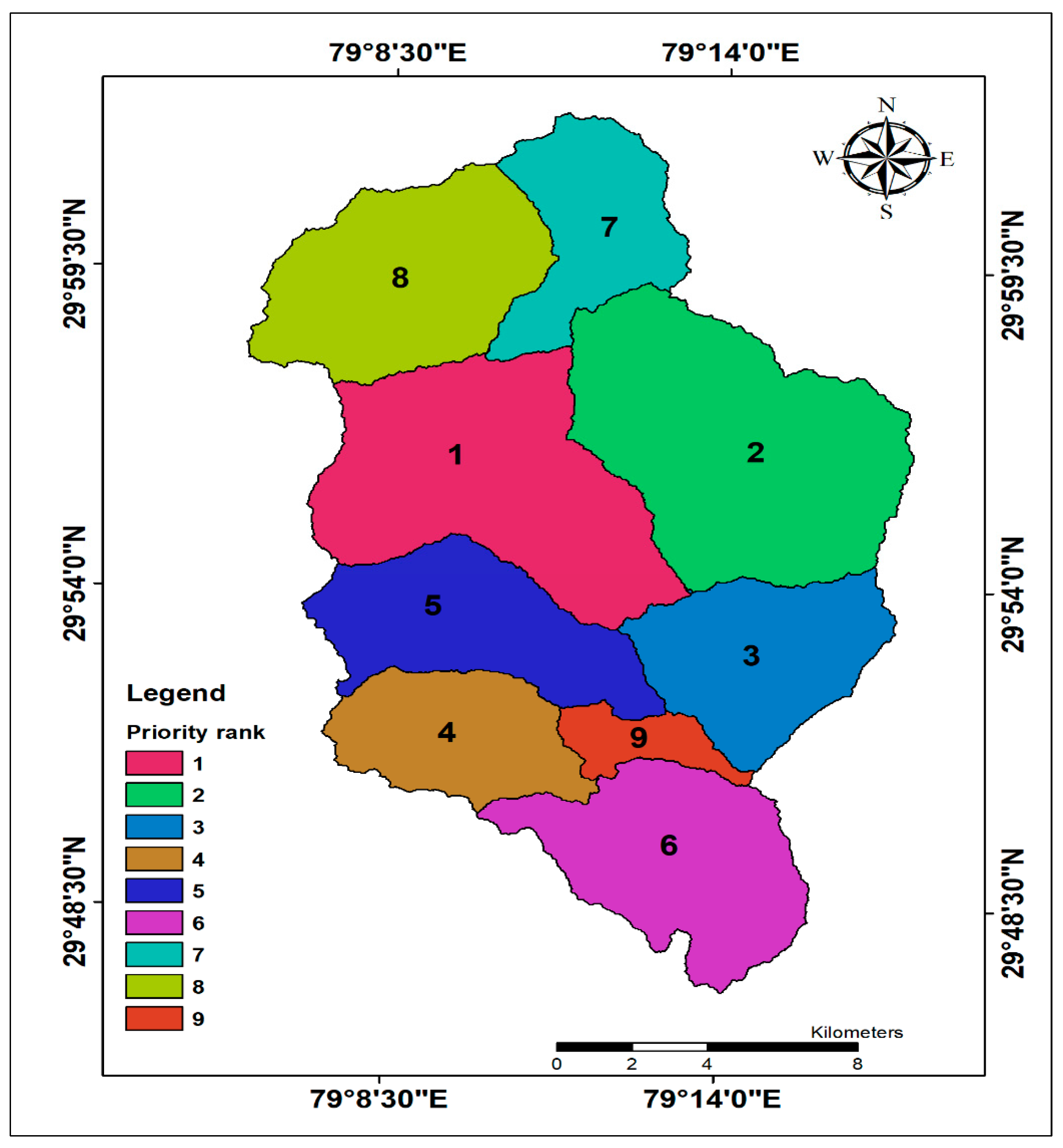
| Sub-Watershed | Compound Factor | Priority Rank |
|---|---|---|
| SW-1 | 6.235 | 6 |
| SW-2 | 8.276 | 9 |
| SW-3 | 4.459 | 4 |
| SW-4 | 3.776 | 3 |
| SW-5 | 4.827 | 5 |
| SW-6 | 1.918 | 1 |
| SW-7 | 2.286 | 2 |
| SW-8 | 6.337 | 7 |
| SW-9 | 6.888 | 8 |
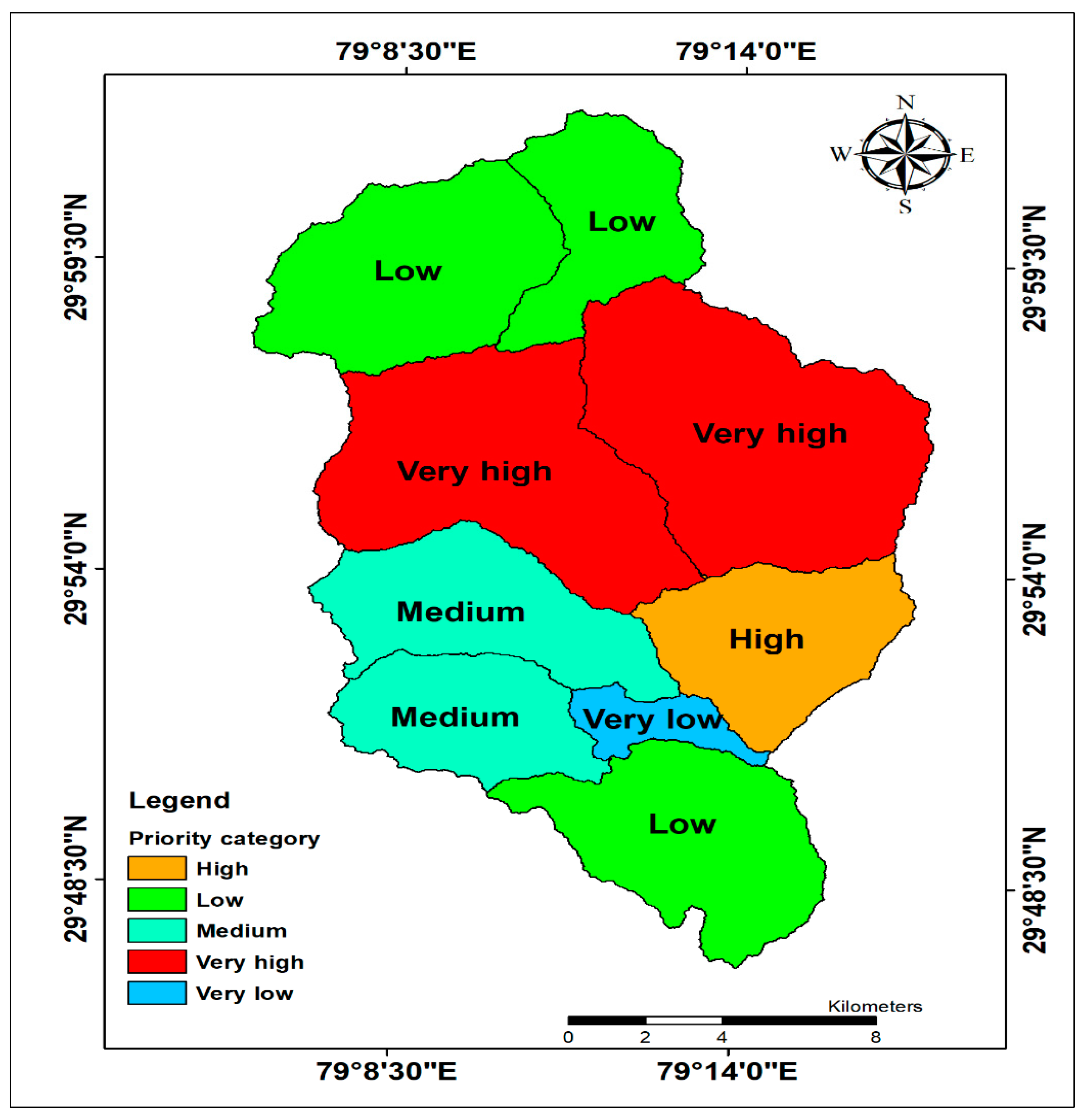
| Sr. No. | Priority Level | Priority Category | Sub-Watershed | Percentage of Area |
|---|---|---|---|---|
| 1 | 1.918 to ≤3.161 | Very high | SW-6, SW-7 | 37.81 |
| 2 | 3.161 to ≤4.403 | High | SW-4 | 9.53 |
| 3 | 4.403 to ≤5.646 | Medium | SW-3, SW-5 | 17.73 |
| 4 | 5.646 to ≤6.888 | Low | SW-1, SW-8, SW-9 | 32.52 |
| 5 | >6.888 | Very low | SW-2 | 2.41 |
© 2019 by the authors. Licensee MDPI, Basel, Switzerland. This article is an open access article distributed under the terms and conditions of the Creative Commons Attribution (CC BY) license (http://creativecommons.org/licenses/by/4.0/).
Share and Cite
Malik, A.; Kumar, A.; Kushwaha, D.P.; Kisi, O.; Salih, S.Q.; Al-Ansari, N.; Yaseen, Z.M. The Implementation of a Hybrid Model for Hilly Sub-Watershed Prioritization Using Morphometric Variables: Case Study in India. Water 2019, 11, 1138. https://doi.org/10.3390/w11061138
Malik A, Kumar A, Kushwaha DP, Kisi O, Salih SQ, Al-Ansari N, Yaseen ZM. The Implementation of a Hybrid Model for Hilly Sub-Watershed Prioritization Using Morphometric Variables: Case Study in India. Water. 2019; 11(6):1138. https://doi.org/10.3390/w11061138
Chicago/Turabian StyleMalik, Anurag, Anil Kumar, Daniel Prakash Kushwaha, Ozgur Kisi, Sinan Q. Salih, Nadhir Al-Ansari, and Zaher Mundher Yaseen. 2019. "The Implementation of a Hybrid Model for Hilly Sub-Watershed Prioritization Using Morphometric Variables: Case Study in India" Water 11, no. 6: 1138. https://doi.org/10.3390/w11061138