Wake Effect Assessment in Long- and Short-Crested Seas of Heaving-Point Absorber and Oscillating Wave Surge WEC Arrays

Abstract

In the recent years, the potential impact of wave energy converter (WEC) arrays on the surrounding wave field has been studied using both phase-averaging and phase-resolving wave propagation models. Obtaining understanding of this impact is important because it may affect other users in the sea or on the coastline. However, in these models a parametrization of the WEC power absorption is often adopted. This may lead to an overestimation or underestimation of the overall WEC array power absorption, and thus to an unrealistic estimation of the potential WEC array impact. WEC array power absorption is a result of energy extraction from the incoming waves, and thus wave height decrease is generally observed downwave at large distances (the so-called “wake” or “far-field” effects). Moreover, the power absorption depends on the mutual interactions between the WECs of an array (the so-called “near field” effects). To deal with the limitations posed by wave propagation models, coupled models of recent years, which are nesting wave-structure interaction solvers into wave propagation models, have been used. Wave-structure interaction solvers can generally provide detailed hydrodynamic information around the WECs and a more realistic representation of wave power absorption. Coupled models have shown a lower WEC array impact in terms of wake effects compared to wave propagation models. However, all studies to date in which coupled models are employed have been performed using idealized long-crested waves. Ocean waves propagate with a certain directional spreading that affects the redistribution of wave energy in the lee of WEC arrays, and thus gaining insight wake effect for irregular short-crested sea states is crucial. In our research, a new methodology is introduced for the assessment of WEC array wake effects for realistic sea states. A coupled model is developed between the wave-structure interaction solver NEMOH and the wave propagation model MILDwave. A parametric study is performed showing a comparison between WEC array wake effects for regular, long-crested irregular, and short-crested irregular waves. For this investigation, a nine heaving-point absorber array is used for which the wave height reduction is found to be up to 8% lower at 1.0 km downwave the WEC array when changing from long-crested to short-crested irregular waves. Also, an oscillating wave surge WEC array is simulated and the overestimation of the wake effects in this case is up to 5%. These differences in wake effects between different wave types indicates the need to consider short-crested irregular waves to avoid overestimating the WEC array potential impacts. The MILDwave-NEMOH coupled model has proven to be a reliable numerical tool, with an efficient computational effort for simulating the wake effects of two different WEC arrays under the action of a range of different sea states.

1. Introduction

Wave energy is meant to play a major role in reducing the world’s fossil fuels dependency [1]. Despite its potential, the exploitation of wave energy is a complex and expensive process. Wave energy can be exploited by using wave energy converters (WECs). The kinetic and potential energy of waves is captured by the power-take-off system of the WEC, which is then converted into electricity. There are or have been at least 157 WECs technologies under development [2], with none of them yet reaching commercial stage. Additionally, for wave energy projects to be economically viable, many WECs must be deployed and arranged in WEC arrays to produce large amounts of electricity. A particular concern for the wave energy sector is the potential impact of the WEC array power absorption in the redistribution of wave energy in the lee of the WEC array.

The overall wave power absorption of a WEC array affects the surrounding wave field creating areas of increased and reduced wave energy (areas of increased and decreased wave height). These modifications may have either a positive or negative effect on the surrounding activities and area. The hydrodynamic problem of wave power absorption between the WECs within an array, and between the WECs and the incident wave field is characterized by three different problems, namely: wave reflection, diffraction, and radiation. The superposition of the reflected, diffracted, and radiated wave fields results in a perturbed wave field. The perturbed wave field close to the WECs of the array caused both by WEC–WEC and wave–WEC interactions is often referred to in the literature as the “near field” effects while the propagation of this perturbed wave field at a larger distance from the WEC array e.g., in the coastal zone, is referred to as the “far-field” effects.

The potential coastal impacts of WEC arrays have been studied in the recent years using phase-averaging and phase-resolving wave propagation models. In [3,4,5,6,7,8,9] a phase-averaging wave propagation model is used to study the wave field in the lee of a WEC array. The WECs of the array are implemented as semi-porous grid cells with a fixed wave transmission (and thus wave power absorption) coefficient. This fixed wave transmission coefficient must be calculated either using a different numerical model as in [3] or by wave tank testing as in [5]. Despite that, without experimental validation it is difficult to assess the accuracy of these models. As pointed out in [10] these transmission coefficients depend on the wave frequency, wave direction, and amplitude. To overcome this limitation [11] improved the fixed wave transmission coefficient introducing a wave frequency and direction dependency mirroring the physics of a real WEC.

In a similar way [12,13] used the phase-resolving mild-slope wave propagation model, MILDwave, to study “far-field” effects of WEC arrays by simplifying each WEC as a frequency-dependent wave power absorbing obstacle. The WEC is implemented in the model using the sponge layer technique ([14]) by assigning to an array of grid cells through coefficients a varying degree of wave reflection, absorption, and transmission. By changing the numerical value of these coefficients in each grid cell or the extent of the grid cells it is possible to replicate the “far-field” impact which the WEC or the WEC array has on the surrounding wave conditions.

Nevertheless, this simplified parametrization of the wave power absorbed by WECs does not take into account the wave-structure interactions due to wave diffraction and radiation between the different WECs modelled as indicated by [15]. Therefore it is not possible to accurately model the “near field” effects, especially for closely spaced WEC arrays. This inaccuracy may lead to an overestimation or underestimation of the WEC array power absorption and consequently an unrealistic estimation of the “far-field” effects in the coastal zone. Additionally, these models depend on the accuracy of the experimental or numerical tests used to tune the internal semi-porous and transmission grid cell coefficients.

Recent studies by the Coastal Engineering Research Group of Ghent University attempted to overcome the limitations of parametric characterization of WEC arrays in wave propagation models by solving the “near field” effects accurately in wave-structure interaction solvers. This has led to coupled models where a wave-structure interaction solver is used to calculate the hydrodynamic interactions in a small domain nested in a wave propagation model. Afterwards, the “near field” information is transferred to the wave propagation model that calculates the wave propagation over a large domain with minimal computational effort. This approach has been used by [14,16,17,18,19,20] to model WEC (arrays) of heaving-point absorbers using the boundary elements methods (BEM) solver NEMOH and coupling it into wave propagation models such as OceanWave3D [21] and MILDwave [22], respectively. The results of these investigations showed a minimal impact on the “far-field” effects than predicted from just applying wave propagation models. Similarly, [23,24,25] used a coupled model to study oscillating wave surge WEC arrays in shallow water coastal areas showing a significant, but lower impact than that predicted by only wave propagation models.

To our knowledge, all “far-field” field effects studies currently available in the literature are carried out using unidirectional regular or irregular long-crested waves. As pointed out in [26] the performance of WEC arrays changes in short-crested sea states. A change in the performance of the WEC array has an impact in the “far-field” effects. The present investigation introduces a parametric study of the magnitude of “far-field” effects of WEC arrays under the effect of regular waves, and long-crested and short-crested irregular waves. The MILDwave-NEMOH coupled model presented in [18] and validated in [19] is employed. Two types of WECs with different absorption principles have been chosen and tested individually and for different WEC array configurations. To our knowledge this novel study is the first one focusing on the comparison of far-field WEC array effects of WECs under different wave types, and especially short-crested waves for a coupled model.

The structure of the paper is as follows: Section 1 provides a short overview of the state-of-the-art and presents the problem statement. Section 2 presents the coupled model used for the parametric study. Section 3 includes a detailed description of the parametric study and the numerical implementation. Results are presented in Section 4. In Section 5 the need for studying “far-field” effects of WEC arrays under short-crested irregular waves is discussed. Finally, the conclusions of this and future work are drawn in Section 6.

2. MILDwave-NEMOH Coupled Model

2.1. Basis of the MILDwave-NEMOH Coupled Model

In this section, the coupled model used in this research is briefly presented. The coupled model is based on a generic coupling methodology first introduced by [14,16,27], who presented a coupled model between the wave propagation model MILDwave and the wave-structure interaction solver WAMIT [28]. The objective of the coupling methodology is to obtain the total wave field around a (group of) structure(s), as a superposition of the incident and the perturbed wave fields. The incident wave field propagation and transformation is calculated over a large domain using a wave propagation numerical model. The perturbed wave field is simulated using a wave-structure interaction solver over a restricted domain around the structure(s), namely the coupling region.

In [18,19] the aforementioned coupling methodology is applied between the wave propagation model, MILDwave, and the waves-structure interaction solver, NEMOH. The MILDwave-NEMOH coupled model is implemented in four steps performing three different simulations:

• A first simulation is performed in MILDwave to obtain the incident wave field in the time-domain, without any floating structure in the numerical basin. The wave characteristics at the coupling location are computed and used as input values for NEMOH.
• A second simulation is performed in NEMOH to calculate the perturbed wave field around the floating structure at the coupling location in the frequency-domain.
• A third simulation is performed in MILDwave to obtain the perturbed wave field in the time-domain. The perturbed wave field from NEMOH is transformed from the frequency-domain to the time-domain and coupled into MILDwave by prescribing an internal wave generation boundary.
• Finally, the total wave field is obtained as the combination of the incident and perturbed wave fields calculated in MILDwave in the time-domain.

This resulted in a one-way coupled model, namely the MILDwave-NEMOH coupled model, that has been numerically and experimentally validated for regular and long-crested irregular waves [18,19].

2.2. The Wave Propagation Model MILDwave

The wave propagation model used within this research is the mild-slope model MILDwave developed at the Coastal Engineering Research Group of Ghent University in Belgium ([14,22]). In recent years, MILDwave has been widely used in the modelling of “far-field” effects of WEC arrays ([12,13,17,25,29]) as it has proven to be a robust and efficient numerical model for calculating wave propagation through WEC arrays and over large coastal areas.

MILDwave is a phase-resolving model based on the depth-integrated mild-slope equations of [30] given in Equations (1) and (2). MILDwave describes the wave transformations (shoaling and refraction) of regular, irregular, and short-crested waves with a narrow frequency band propagating above mildly varying bathymetries.

$$\frac{\partial \eta }{\partial t}=\frac{{\omega }^2-k^{2}C{C}_g}{g}\varphi -\nabla (\frac{C{C}_g}{g}\nabla \varphi ),$$

(1)

$$\frac{\partial \varphi }{\partial t}=-g\eta ,$$

(2)

with $\eta$ the surface elevation, g the acceleration of gravity, t the time, $\varphi$ is the velocity potential, C the phase velocity and $C_g$ the group velocity for a wave with wave number, k, and angular frequency, $\omega$. MILDwave uses an internal wave generation line near the offshore boundary by applying the source term addition method introduced by [31] where the source term propagates with the energy velocity, $C_e$. $C_e$ is the velocity of disturbance caused by the incident wave. According to this method, an additional surface elevation with the desired energy ${\eta }^{\ast }$ is added to the calculated surface elevation $\eta$ at the wave generation line for each time step and is given by Equation (3):

$${\eta }^{\ast }=2{\eta }_I\frac{C_e\Delta t}{\Delta x}cos\theta ,$$

(3)

where $\Delta x$ is the grid size in the x-axis, $\Delta t$ is the time step, $\theta$ is the angle of the incident wave ray from x-axis, ${\eta }_I$ is the incident wave surface elevation.

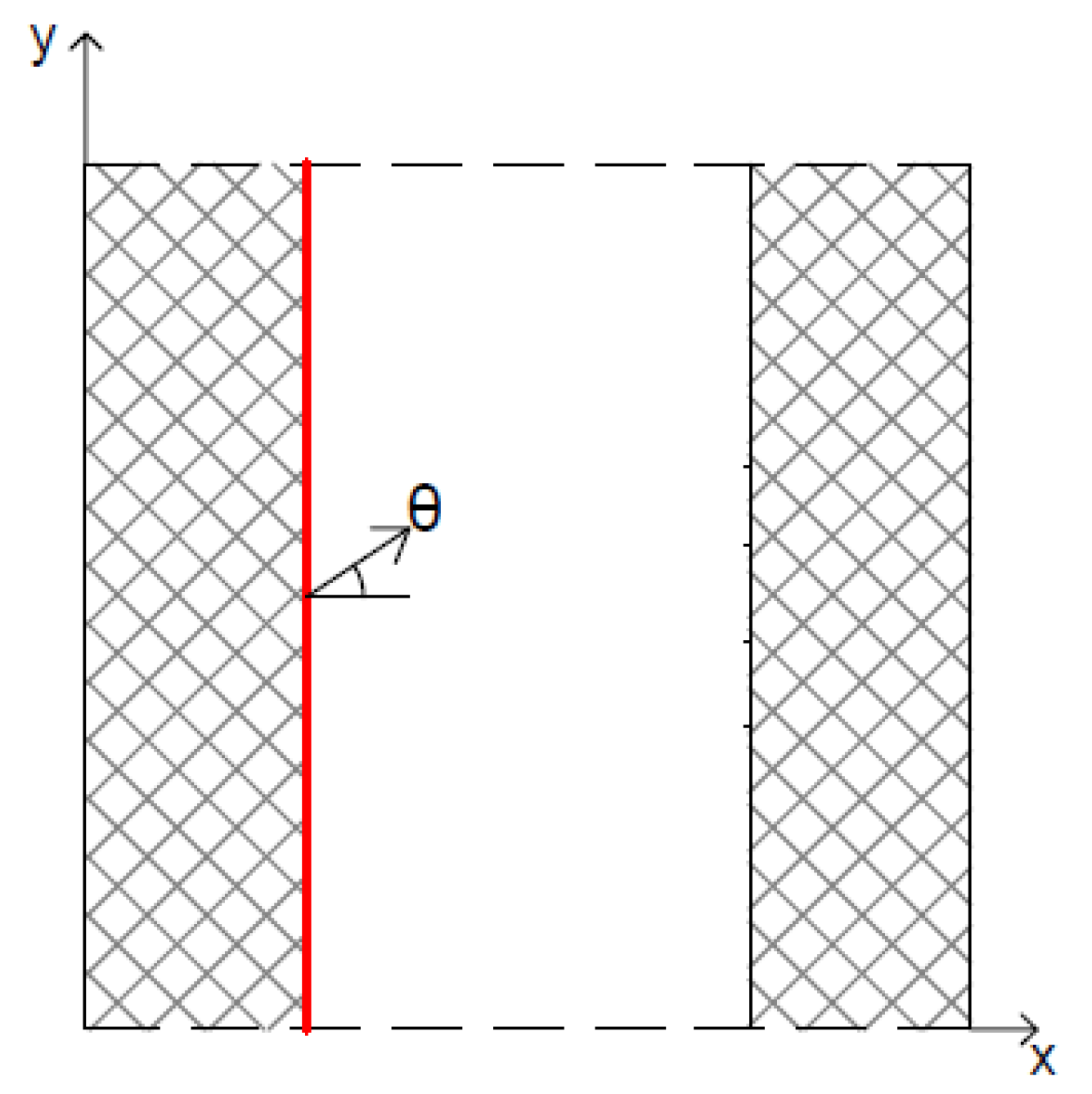
In the MILDwave-NEMOH coupled model a single internal wave generation line combined with periodic lateral boundaries is recently used. Periodic lateral boundaries have been implemented by [32] allowing the model to create homogeneous wave fields of oblique regular, long-crested, and short-crested irregular waves. Figure 1 shows the schematics of internal wave generation using a single wave generation line parallel to the y-axis combined with periodic lateral boundaries at the lateral sides of the numerical domain (indicated by dashed lines at the top and bottom part of Figure 1). The information reaching one end of the domain enters the opposite end.

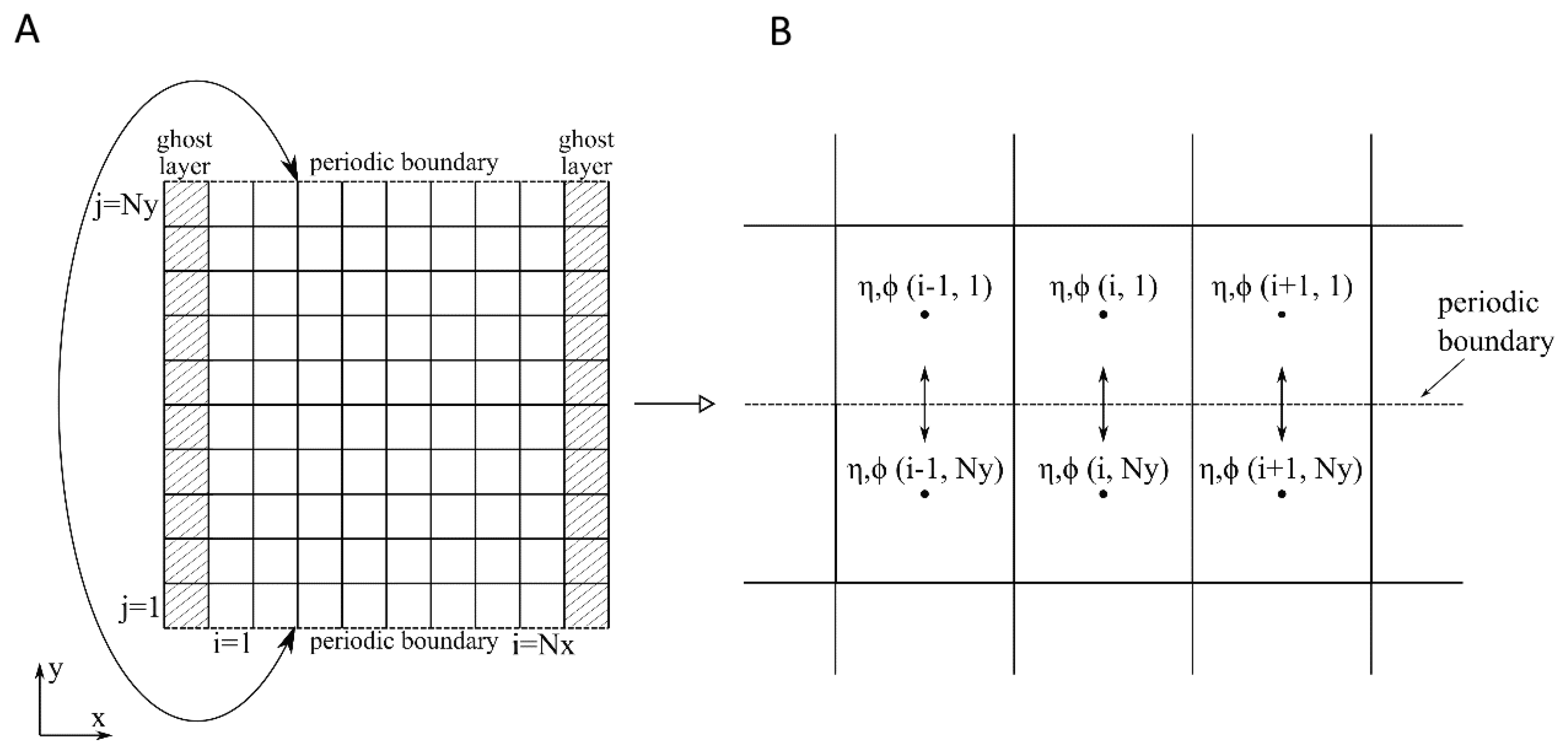
Figure 2 shows a schematic of the periodic lateral boundaries implementation. A layer of additional grid cells is present next to each vertical boundary, acting as fully reflective walls while the periodic boundaries are represented by dashed lines in the x-axis direction (Figure 2A). At the position of the periodic boundaries, Equations (1) and (2) are solved as if the horizontal boundaries were next to each other (Figure 2B). The bathymetry close to both lateral boundaries has to be identical between each other to ensure continuity.

2.3. The Wave-Structure Interaction Solver, NEMOH

The wave-structure interaction solver employed to solve the diffraction/radiation problem and deliver the perturbed wave field around the floating WEC is the open-source potential flow BEM solver NEMOH, developed at Ecole Centrale de Nantes [33]. NEMOH is based on linear potential flow theory [34], and employs the following assumptions:

• The flow is inviscid.
• The flow is irrotational.
• The fluid is incompressible.
• The motion amplitudes of the modelled floating bodies are much smaller than the wavelength.
• The sea bottom is flat.

Under these conditions the water velocity, $\overrightarrow{u}$, can be expressed in terms of the velocity potential, $\varphi (x,y,z,t)$, according to:

$$\overrightarrow{u}=\nabla \varphi .$$

(4)

Linear potential flow theory has hitherto been used in most of the investigations into WEC array modelling, for example see [17,26,35,36]. Due to the principle of superposition, linear potential theory allows for the separation of the total wave field into the following components of the wave velocity potential:

$${\varphi }_{tot}(x,y,z)={\varphi }_I+{\varphi }_{diff}+{\displaystyle \sum _j^6}{\varphi }_{rad},$$

(5)

where ${\varphi }_{tot}$ is the total wave velocity potential, ${\varphi }_I$ is the incident wave velocity potential, ${\varphi }_{diff}$ is the diffracted wave velocity potential and ${\sum }_j^6{\varphi }_{rad}$ is the sum of the radiated wave velocity potentials for each degree of freedom (DOF) of motion of the structure(s).

2.4. Generation of the Incident Wave Field

The incident wave field is calculated using the wave propagation model MILDwave in the time-domain. It is possible to simulate regular waves, and long-crested and short-crested irregular waves in MILDwave. However, for the coupled model it is not possible to perform a direct calculation of irregular waves using a one-way coupling. This is because it is necessary to ensure the correct matching between each incident and perturbed wave regular component. Consequently, in this section details are provided on obtaining the incident regular waves and correctly calculating the irregular waves as a superposition of different linear regular wave components.

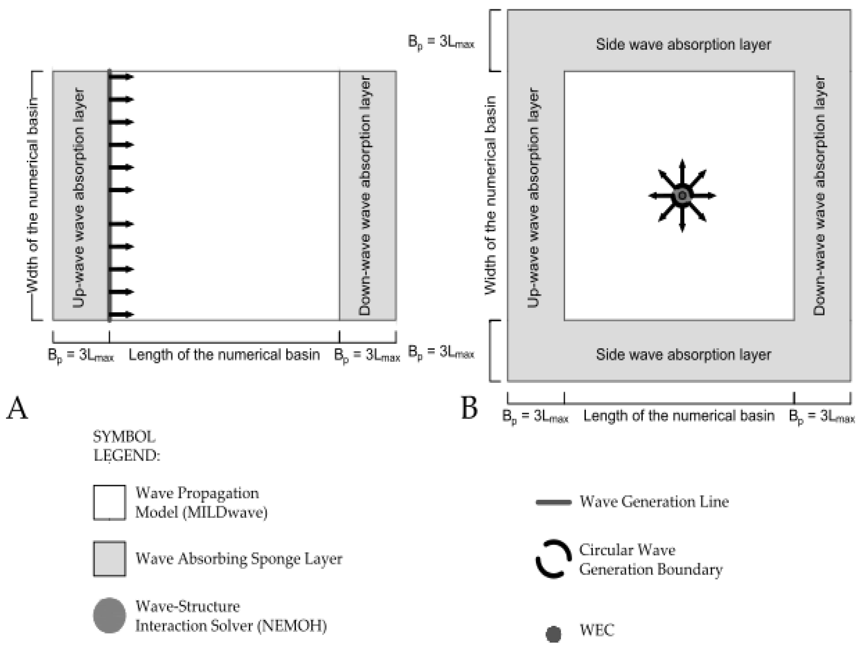
The incident wave field for a linear regular wave is generated intrinsically in MILDwave. The numerical set-up of MILDwave is illustrated in Figure 3A. Waves are generated along a linear offshore wave generation boundary (e.g., as illustrated in Figure 1) by applying the boundary condition of linear regular waves’ generation:

$${\eta }_{I,reg}(x,y,t)=acos(\omega t-k(xcos\left(\theta \right)+ysin\left(\theta \right))),$$

(6)

where ${\eta }_{I,reg}$ is the incident regular wave surface elevation and a is the wave amplitude. To minimize unwanted wave reflection, absorption layers are placed downwave and up-wave in the numerical wave basin.

By applying the superposition principle, a first order irregular wave is represented as the finite sum of $N_f$ regular wave components characterized by their wave amplitude, $a_j$, and wave period, $T_j$, derived from the wave spectral density, $S_j$:

$${\eta }_{I,irr}(x,y,t)={\displaystyle \sum _{j=1}^N}{a}_{j}cos({\omega }_{j}t-k_j(xcos\left({\theta }_j\right)+ysin\left({\theta }_j\right))+{\phi }_j),$$

(7)

where

$$a_j=\sqrt{2S_j\left(f_j\right)·\Delta f_j},$$

(8)

where ${\eta }_{I,irr}$ is the incident irregular wave surface elevation and $a_j$ is the wave amplitude, ${\omega }_j$ is the wave angular frequency, $f_j$ is the wave frequency, $k_j$ is the wave number, ${\theta }_j$ is the wave direction and ${\phi }_j$ is the incident phase angle, of each wave frequency component j. ${\phi }_j$ is selected randomly between $-\pi$ and $\pi$ to avoid local attenuation of ${\eta }_{I,irr}$.

To generate a long-crested irregular wave, ${\theta }_j$ is equal to the mean direction of wave propagation, ${\theta }_{mean}$, for all wave frequency components. In the case of short-crested waves the wave directions, ${\theta }_j$, introduced in Equation (7) are obtained for each frequency using periodic boundaries and the Sand and Myneet [37] method.

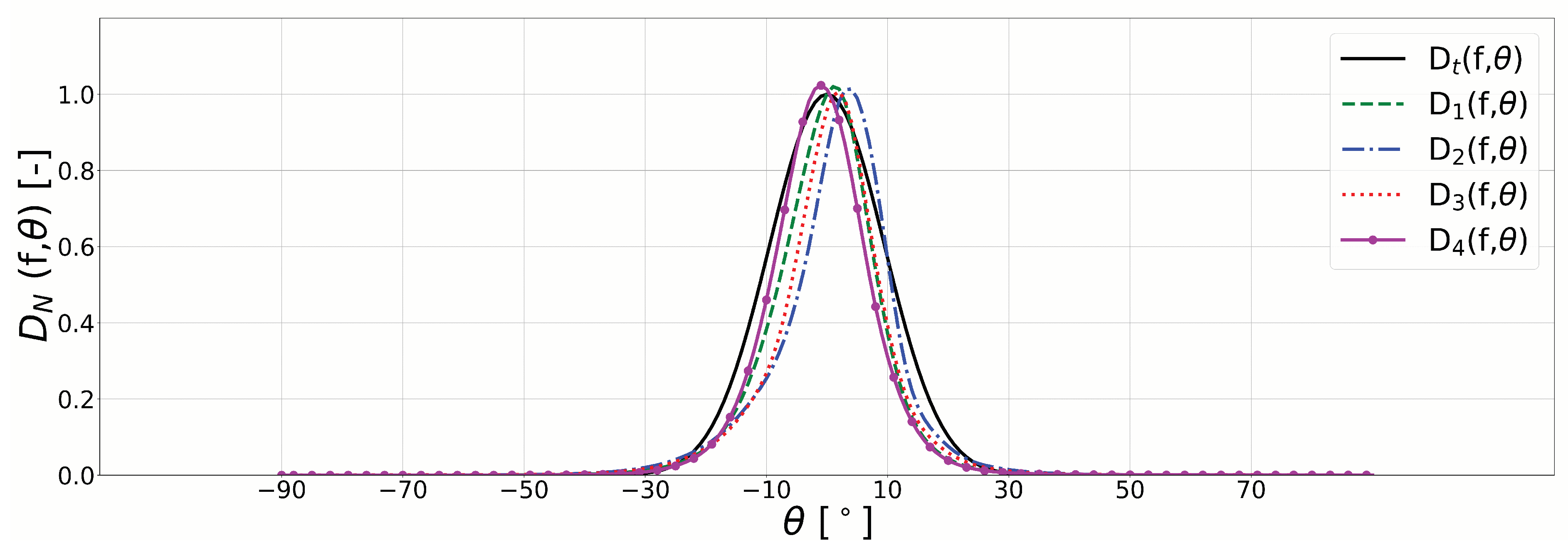
According to this method, the wave spectrum is discretized in $N_f$ frequency components. The wave propagation angles ${\theta }_j$ are selected randomly according to the cumulative distribution function of the directional spreading function, $D(f,\theta )$, and are assigned to each wave frequency component. This model provides an accurate representation of the targeted spreading function shape as shown in [32]. The spreading function of Frigaard [38] is employed:

$$D(f,\theta )=\frac{1}{\sqrt{\pi }}\frac{\Gamma (s_1+1)}{\Gamma (s_1+\frac{1}{2})}{cos}^{2s_1}(\theta -{\theta }_{mean}),$$

(9)

with,

$$-\frac{\pi }{2}<\theta -{\theta }_{mean}<\frac{\pi }{2},$$

(10)

where $s_1$ is the directional spreading parameter, $\Gamma$ is the Gamma function.

Hence, the values of $s_1$ can be determined for different directional spreading, given by:

$${\sigma }_{\theta }=\sqrt{2-\frac{2{\Gamma }^2\left(s_1+1\right)}{\Gamma \left(s_1+\frac{1}{2}\right)\Gamma \left(s_1+\frac{3}{2}\right)}},$$

(11)

where ${\sigma }_{\theta }$ is the standard deviation of the directional spreading.

2.5. Calculation of the Perturbed Wave Field

The perturbed wave field in the time-domain for a regular wave is obtained in two steps and the employed numerical set-up is illustrated in Figure 3B. First, a frequency-dependent simulation is performed using NEMOH to obtain the complex perturbed wave field around the (group of) structure(s). NEMOH resolves the wave frequency-dependent wave radiation problem for each (of the) structure(s) and the diffraction (including radiation) over a predetermined numerical grid with the wave phase angle $\phi =0$ at the center of the domain. The resulting radiated and diffracted wave fields for each frequency, $f_j$, depend on the shape and number of floating structure(s), the number of DOF considered, the local constant water depth and the wave period.

NEMOH provides the complex radiated wave field as a summation of the radiated wave field for each floating structure. The diffracted wave field is given for all structures. Equations (12) and (13) describe the complex radiated and diffracted wave fields, respectively:

$${\eta }_{rad}={\displaystyle \sum _k^J}ia\omega {\tilde{X}}_k\left(\omega \right){\left|{\eta }_{rad}\right|}_k{e}^{i{\phi }_{rad,k}},$$

(12)

$${\eta }_{diff}=a\left|{\eta }_{diff}\right|e^{i{\phi }_{diff}},$$

(13)

where ${\eta }_{rad}$ is the radiated wave field, ${\eta }_{diff}$ is the diffracted wave field, i is the imaginary number part, ${\phi }_{rad}$ and ${\phi }_{diff}$ correspond to the radiated and diffracted wave phase angle, respectively, J is the total number of floating WECs and $\tilde{X}$ is the Response Amplitude Operator (RAO) for one DOF of the J WECs given by:

$$\tilde{X}={\tilde{F}}_{ex}·{\left[-(\mathit{m}+{\mathit{M}}_{\mathit{A}}){\omega }^2-i\omega ({\mathit{B}}_{\mathit{hyd}}+{\mathit{B}}_{\mathit{PTO}})+{\mathit{K}}_{\mathit{H}}\right]}^{-1},$$

(14)

here ${\tilde{F}}_{ex}$ is the excitation force vector of the J WECs, $\mathit{m}$ is the WEC’s mass matrix, ${\mathit{M}}_{\mathit{A}}$ is the added mass matrix, ${\mathit{B}}_{\mathit{hyd}}$ is the hydrodynamic damping coefficient matrix, ${\mathit{B}}_{\mathit{PTO}}$ is the Power Take-Off (PTO) damping coefficient matrix and ${\mathit{K}}_{\mathit{H}}$ is the hydrodynamic stiffness matrix.

The radiated and diffracted complex wave fields are added to obtain the perturbed wave field, ${\eta }_{pert}$:

$${\eta }_{pert}={\eta }_{diff}+{\eta }_{rad}.$$

(15)

Secondly, the perturbed wave field is transformed from the frequency-domain to the time-domain and imposed into MILDwave using an internal circular (or in other cases rectangular) wave generation boundary (Figure 3B). To ensure phase matching between the incident and perturbed wave fields, the phase angle obtained from NEMOH has to be corrected with the phase angle of the incident regular wave in the center of the internal wave generation boundary. Waves are forced away from the wave generation boundary by imposing values of free surface elevation ${\eta }_b(x,y,t)$ as described by Equation (16):

$${\eta }_b(x,y,t)=a_{I,c}\left|{\eta }_{pert}\right|cos({\phi }_{pert,NM,c}+{\phi }_{I,c}-\omega t),$$

(16)

where ${\eta }_b$ is the wave surface elevation at the internal wave generation boundary, ${\eta }_{pert}$ is the perturbed complex wave field from the frequency-domain, $a_{I,c}$ and ${\phi }_{I,c}$ are the wave amplitude and the wave phase angle of the incident wave at the location of the internal wave generation boundary, respectively. ${\phi }_{pert,NM}$ is the phase angle of the perturbed wave at the internal wave generation boundary, c. To avoid unwanted wave reflection, wave absorption layers or relaxation zones are implemented up-wave, downwave and in the sides of the MILDwave numerical domain (Figure 3B).

As in the case for the calculation of the irregular incident wave field, the irregular perturbed wave field is calculated as the finite sum of N regular perturbed wave components characterized at the center of the wave generation boundary by their wave amplitude, $a_{c,j}$, derived from the wave spectrum:

$${\eta }_{pert,irr}(x,y,t)={\displaystyle \sum _{j=1}^N}{a}_{c,j}\left|{\eta }_{pert}\right|cos({\phi }_{pert,NM,c,j}+{\phi }_{I,c,j}-{\omega }_{j}t),$$

(17)

where

$$a_{c,j}=\sqrt{2S_{c,j}\left(f_j\right)·\Delta f_j},$$

(18)

and ${\eta }_{pert,irr}$ is the perturbed irregular wave surface elevation where $S_{c,j}$ is the spectral density, and ${\phi }_{I,c,j}$ is the incident phase angle and ${\phi }_{pert,NM,c,j}$ is the perturbed phase angle in NEMOH of each frequency component at the internal wave generation boundary, c. ${\phi }_{I,c,j}$ is selected randomly between $-\pi$ and $\pi$ to avoid local attenuation of the wave surface elevation.

This methodology for calculating irregular waves is valid both for long-crested and short-crested waves. The phase angle of the perturbed wave obtained in NEMOH is dependent on the incident wave direction of each wave frequency. Thus, the wave direction of each frequency is implicitly considered when prescribing the internal wave generation boundary and forcing away the perturbed wave field. In the case of long-crested waves it corresponds with the mean direction, while in the case of short-crested waves each direction corresponds with the random direction assigned to each regular wave component.

2.6. Calculation of the Total Wave Field

The regular total wave field is obtained as the superposition of the incident and perturbed regular wave fields obtained in the MILDwave numerical domain as:

$${\eta }_{tot,reg}(x,y,t)={\eta }_{I,reg}(x,y,t)+{\eta }_{pert,reg}(x,y,t),$$

(19)

where ${\eta }_{tot,reg}$ is the total regular wave surface elevation, and ${\eta }_{I,reg}$ and ${\eta }_{pert,reg}$ are the incident and perturbed regular wave surface elevation.

Consequently, the irregular total wave field is obtained as the superposition of the irregular incident and perturbed wave fields, which are at the same time obtained as a superposition of N regular wave simulations:

$${\eta }_{tot,irr}(x,y,t)={\displaystyle \sum _j^N}{\eta }_{I,reg,j}(x,y,t)+{\displaystyle \sum _j^N}{\eta }_{pert,reg,j}(x,y,t),$$

(20)

where ${\eta }_{tot,irr}$ is the total irregular wave surface elevation, and ${\eta }_{I,reg,j}$ and ${\eta }_{pert,reg,j}$ are the incident and perturbed wave surface elevations of each $f_j$, respectively.

3. Numerical Framework

In this section, a numerical test case is presented to compare the “far-field” effects of WEC arrays under the effect of regular waves, and long-crested and short-crested irregular waves. Firstly, the different WECs studied and their array configurations are introduced. Secondly the used wave conditions are defined. Thirdly, the numerical set-up in the MILDwave-NEMOH coupled is described.

3.1. Modelled WECs and Array Layout

Two of the most promising and investigated WEC types, with several prototypes developed over recent years [2], have been chosen:

• Heaving Cylindrical Wave Energy Converter (HCWEC): is a disc shaped heaving buoy WEC with a diameter, ∅, of 20.0 m, a height, $h_{HC}$, of 4.0 m, and a draft, $d_{HC}$, of 2.0 m. HCWECs are designed to be deployed at water depths of around 30.0 m.
• Oscillating Wave Surge Wave Energy Converter (OSWEC): the second WEC chosen is a bottom-fixed pitching flap driven by the surge motion of the waves. OSWECs are designed to be deployed in shallow water at depths of 10.0–20.0 m. The simulated OSWEC has dimensions of 20.0 m width, $w_{OS}$, 1.0 m thickness, $t_{OS}$, and 12.0 m height, $h_{OS}$. It is hinged at the seabed with pitching motion about its bottom end.

Firstly, each WEC is modelled independently over a constant bathymetry with a water depth corresponding to that at the expected deployment site. Secondly, each WEC is modelled for two staggered array configurations of five and nine WECs. This type of configuration has been selected as it has been used in a wide number of studies. It has shown to maximize the total power output of the WEC array, and thus maximizes the array impact on the surrounding wave field. Figure 4A shows the staggered configuration of 5 HCWECs (referred to as “H1”) in green, and 9 HCWECs (referred to as “H2”) combining green and black. Identically, Figure 4B shows the staggered configuration of 5 OSWECs (referred to as “O1”) in green, and 9 OSWECs (referred to as “O2”) combining green and black.

3.2. Wave Conditions

Regular waves are obtained using a wave height of $H=2.0$ m and a wave period of $T=8.0$ s. Long-crested and a short-crested irregular sea states are generated using a significant wave height of $H_s=2.0$ m and a wave peak period of $T_p=8.0$ s. A Pierson-Moskovitz (abbreviated as P-M) spectrum is used in Equations (7) and (8). The P-M irregular wave spectrum is defined by Equation (21):

$$S\left(f\right)=\frac{B}{f^5}{e}^{-\frac{C}{f^4}},$$

(21)

where

$$B=\frac{5}{16}\frac{H_s^2}{T_p^4},$$

(22)

$$C=\frac{5}{4}\frac{1}{T_p^4}.$$

(23)

For long-crested irregular waves the wave direction of each component is equal to the mean wave propagation direction (${\theta }_j={\theta }_{mean}$). In the case of short-crested waves the wave directions, ${\theta }_j$, introduced in Equation (7) are obtained for each frequency component applying the Sand and Mynnet method [37] introduced in Section 2.4. The values of $s_1$ and ${\sigma }_{\theta }$ are determined for swell waves:

$$s_1=15.8\to {\sigma }_{\theta }={10}^{\circ }.$$

(24)

3.3. Numerical Set-Up

As indicated in Section 2 three different simulations are performed in the MILDwave-NEMOH coupled model: an incident and a perturbed wave simulation in MILDwave, and a perturbed wave simulation in NEMOH.

For the incident wave simulation in MILDwave an effective domain of length, $l_{MW}$ = 2000 m and width, $w_{MW}$ = 2000 m is used. The water depth, d, is set to 30.0 m and 10.0 m for the HCWECs and OSWECs, respectively. Waves are generated using a linear wave generation line located at the left side of the numerical domain. To avoid reflection, two equally sized wave absorbing sponge layers are placed up-wave (left) and downwave (right), as indicated in Figure 3A. The length of the sponge layers, $B_p$, is calculated using the maximum wavelength L of the discretized spectra for irregular waves, $L_{max}$. $L_{max}$ is the wavelength of the regular wave with the highest wave period of the discretized spectrum, $T_{max}$. The length of the sponge layer is then equal to $B_p=3L_{max}$.

For the perturbed wave simulation in MILDwave, the same effective domain dimensions are used. Effective domain is the area of the numerical wave basin that is not covered by sponge layers (e.g., white area in Figure 3A,B). Waves are generated using an internal wave generation circle located at the center of the effective domain. The radius of the internal wave generation boundary, $R_c$, must be defined in relation to the WEC(s) geometry that are placed inside it. A minimum distance from the center of the internal wave generation boundary to the outside limit needs to be equal to the distance from its center to the furthest WEC of the array plus a wave propagation area. This leads to an $R_c$ of 58.0 m, 134.0 m and 190.0 m for one, five, and nine WECs, respectively. To avoid reflection and the transmission of the perturbed wave across the periodic boundaries, two additional sponge layers are placed at the top and bottom of the numerical domain (Figure 3B).

The rest of the MILDwave simulation parameters have been summarized in

Table 1. MILDwave simulation parameters for the MILDwave-NEMOH coupled model.

Regular Waves	Long-Crested Irregular Waves	Short-Crested Irregular Waves
H = $2.0$ m	$H_s=2.0$ m	$H_s$ = $2.0$ m
$T=8.0$ s	$T_p=8.0$ s	$T_p$ = $8.0$ s
$\theta ={30.0}^{\circ }$	$\theta ={30.0}^{\circ }$	$\theta ={30.0}^{\circ }$
$l_{MW}$ = 2000.0 m	$l_{MW}$ = 2000.0 m	$l_{MW}$ = 2000.0 m
$w_{MW}$ = 2000.0 m	$w_{MW}$ = 2000.0 m	$w_{MW}$ = 2000.0 m
-	Pierson–Moskowitz Spectrum	Pierson–Moskowitz Spectrum
-	$N_f$ = 20	$N_f$ = 50
-	$s_1$ = 0.0	$s_1$ = 15.8
$d_x$ = L/30 = 3.0 m	$d_x$ = $L_p$/30 = 3.0 m	$d_x$ = $L_p$/30 = 3.0 m
$d_y$ = L/30 = 3.0 m	$d_y$ = $L_p$/30 = 3.0 m	$d_y$ = $L_p$/30 = 3.0 m
$t_{sim}$ = 600 s	$t_{sim}$ = 4000 s	$t_{sim}$ = 5000 s
$\Delta t$ = 0.4 s	$\Delta t$ = 0.4 s	$\Delta t$ = 0.4 s

: type of spectrum, number of regular wave components, $N_f$, directional spreading parameter, $s_1$, grid cell size in x-axis and y-axis, $d_x$ and $d_y$, simulation time, $t_{sim}$, and time step, $\Delta t$.

For the perturbed wave simulation in NEMOH a domain of length, $l_{NM}$ = 400 m and width, $w_{NM}$ = 400 m is used as it is sufficient to fit the different coupling radii used for the MILDwave internal wave generation boundary. The water depth, d, is set to 30.0 m and 10.0 m for the HCWECs and OSWECs, respectively. The HCWEC and OSWEC have been discretized using 200 and 300 panels, respectively. The effect of the WEC’s PTO system is taken into account adding the suitable external damping coefficient, $B_{PTO}$, in the equation of motion (Equation (14)). The optimal $B_{PTO,opt}$ that maximizes the energy conversion for a single WEC in regular waves is used ([39]) using as input the peak angular frequency, ${\omega }_p$. It is derived from the following expression:

$$B_{PTO,opt}=\sqrt{(B_{hyd}^2+{({\omega }_p(m+M_A)-\frac{K_H}{{\omega }_p})}^2)}$$

(25)

This results in a value of $B_{PTO,opt}$=$2.25\times {10}^6\mathrm{kg}·{\mathrm{s}}^{-1}$ and $98.4\times {10}^6\mathrm{kg}·{\mathrm{m}}^2{\mathrm{s}}^{-2}$ for the HCWEC and the OSWEC, respectively. The rest of the NEMOH simulation parameters have been summarized in

Table 2. NEMOH simulation parameters for the MILDwave-NEMOH coupled model.

Regular Waves	Long-Crested Irregular Waves	Short-Crested Irregular Waves
H = $2.0$ m	$H_s=2.0$ m	$H_s$ = $2.0$ m
$T=8.0$ s	$T_p=8.0$ s	$T_p$ = $8.0$ s
$\theta ={30.0}^{\circ }$	$\theta ={30.0}^{\circ }$	$\theta ={30.0}^{\circ }$
$l_{NM}$ = 400.0 m	$l_{NM}$ = 400.0 m	$l_{NM}$ = 400.0 m
$w_{NM}$ = 400.0 m	$w_{NM}$ = 400.0 m	$w_{NM}$ = 400.0 m
-	Pierson–Moskowitz Spectrum	Pierson–Moskowitz Spectrum
-	$N_f$ = 20	$N_f$ = 50
-	$s_1$ = 0.0	$s_1$ = 15.8
$d_x$ = L/30 = 3.0 m	$d_x$ = $L_p$/30 = 3.0 m	$d_x$ = $L_p$/30 = 3.0 m
$d_y$ = L/30 = 3.0 m	$d_y$ = $L_p$/30 = 3.0 m	$d_y$ = $L_p$/30 = 3.0 m

: type of spectrum, number of regular wave components, $N_f$, directional spreading parameter, $s_1$, grid cell size in x-axis and y-axis, $d_x$ and $d_y$, simulation time, $t_{sim}$, and time step, $\Delta t$.

3.4. Test Cases

Combining the different wave conditions, WEC types and WEC array layouts a set of numerical test cases has been generated and summarized in

Table 3. Numerical test cases for the comparison of “far-field” effects comparison.

Test Case	Wave Type	WEC (array)
1	Regular	Single HCWEC
2	Regular	H1 array layout
3	Regular	H2 array layout
4	Regular	Single OSWEC
5	Regular	O1 array layout
6	Regular	O2 array layout
7	Irregular long-crested	Single HCWEC
8	Irregular long-crested	H1 array layout
9	Irregular long-crested	H2 array layout
10	Irregular long-crested	Single OSWEC
11	Irregular long-crested	O1 array layout
12	Irregular long-crested	O2 array layout
13	Irregular short-crested	Single HCWEC
14	Irregular short-crested	H1 array layout
15	Irregular short-crested	H2 array layout
16	Irregular short-crested	Single OSWEC
17	Irregular short-crested	O1 array layout
18	Irregular short-crested	O2 array layout

:

4. Results

4.1. $K_d$ Disturbance Coefficient for Short-Crested Irregular Waves

Before performing the parametric study introduced in Section 3 the capabilities of the MILDwave-NEMOH coupled model to simulate short-crested irregular waves are here discussed. The methodology introduced in Section 2.4 uses periodic boundaries and the Sand and Mynett method to generate short-crested irregular waves as a superposition of regular wave components. On one hand, the use of periodic boundaries can lead to erroneous results in the perturbed wave field simulation with the perturbed wave transferring along the lateral boundaries of the numerical domain. On the other hand, the Sand and Mynnet method assigns a wave direction ${\theta }_j$ for each wave frequency component of the discretized spectra causing that each simulation generates a different normalized spreading function.

Figure 5 and Figure 6 show the $K_d$ disturbance coefficient results for a single HCWEC interacting with a regular wave with H = 2.0 m and $T=$ 8.0 s with waves propagating from left to right. The $K_d$ disturbance coefficient is defined as the ratio between the numerically calculated local total wave height, $H_{tot}$, and the target wave height, $H_I$, imposed along the linear wave generation boundary:

$$K_d=\frac{H_{tot}}{H_I}$$

(26)

In Figure 5 an internal wave generation line combined with periodic boundaries (as indicated in Figure 1) is used to generated and incident wave with $\theta$ = $0^{\circ }$. In Figure 6 the incident wave angle is changed to $\theta$ = ${30}^{\circ }$. As it can be seen in Figure 5 and Figure 6 two identical results are obtained rotated ${30}^{\circ }$. This indicates that the sponge layers located at the lateral sides of the MILDwave numerical domain are absorbing the perturbed wave transferred between the periodic boundaries. This shows that the use of periodic boundaries does not lead to an erroneous calculation of the total wave field around a WEC (array).

To test the repeatability of short-crested irregular waves sea-state generation, ten different simulations with $H_s$ = 2.0 m, $T_p=8.0$ s and $s_1=15.8$ have been performed using the parameters included in Table 1 for the incident waves. The directional wave spectrum has been measured at the center of the domain by a group of five wave gauges using a “CERC 5” configuration [40]. A normalized spreading function, $D_N(f,\theta )$, close to the theoretical one, $D_t(f,\theta )$, is obtained for all the test cases, $D_1(f,\theta )$ to $D_4(f,\theta )$ as illustrated in Figure 7.

Still, the wave frequencies where the WEC is extracting more energy are not necessarily close to the ${\theta }_{mean}$ as they are randomly assigned. Consequently, an asymmetric diffraction and radiation pattern interacting with the incident wave field is generated. Therefore, for comparing the effect on the total wave field of short-crested irregular waves to those of long-crested waves it is not possible to use a single simulation (one sea-state). An average of the $K_d$ value over a different number of simulations should be used instead, to assess the impact of short-crested waves. In this way, it is possible to account for the different angles of the incident waves of the frequencies of the discretized spectra close to the absorption bandwidth of the WEC(s). There, more energy is extracted from the waves and that is randomly changed in each simulation. Figure 8 shows the $K_{d,avg}$ for a total of M = 10 simulations with a randomly generated directional spectra in each case, using the simulation parameters included in Table 1 and a single HCWEC. It can be seen that $K_{d,avg}$ tends to be symmetric along the x-axis corresponding with ${\theta }_{mean}=0^{\circ }$, with waves propagating from left to right.

For the sake of brevity, in the next sections only $K_d$ results for the 9-OSWEC and the 9-HCWEC array will be illustrated using $K_d$ contour plots and cross-sections along the numerical domain of the coupled model. However, results for all modelled WEC configurations of Table 3 are presented in tables and discussed.

4.2. 9-OSWEC Array

Using the MILDwave-NEMOH coupled model for Test Cases 6, 12, and 18 from Table 3 the total wave field around a 9-OSWEC array is obtained for regular waves, and irregular long-crested and short-crested waves, respectively. $K_d$ disturbance coefficient results obtained for each considered test case are illustrated in Figure 9A, Figure 10A and Figure 11A. The coupling region in the MILDwave-NEMOH coupled model is masked out using a white solid circle and is not considered for the results analysis.

For all here considered test cases is it possible to identify a reflection pattern in front of the 9-OSWEC array with increased values of $K_d$. In the lee of the array, there is a reduction of wave height indicated by reduced values of $K_d$. It can be noticed visually in the $K_d$ contour plots that the wave height variation around the 9-OSWEC array is the highest for regular wave conditions and the lowest for short-crested wave conditions. An increase of 38.99%, 19.00% and 5.00% in $K_d$ in front of the 9-OSWEC array is found for Test Cases 6, 12, and 18, respectively. In the lee of the array there is a decrease of $K_d$ equal to −39.08%, −30.81% and −26.55%, for Test Cases 6, 12, and 18, respectively.

To have a closer look at the $K_d$ results for Test Cases 6, 12, and 18 at one longitudinal and four transversal cross-sections (indicated in Figure 9, Figure 10 and Figure 11) are drawn through: the center of the domain, at y = 0 m (S1) and in the lee of the WEC array, at x = 250 m (W1), at x = 500 m (W2), at x = 750 m (W3) and at x = 1000 m (W4). Again, the coupled zone is masked out in cross-section S1 using gray color (Figure 12A). Figure 12A shows that long-crested and short-crested irregular waves have similar $K_d$ in the lee of the WEC array close the coupling region. However, at larger distances in the lee of the 9-OSWEC array the wave height recovers faster for short-crested waves due to the influence of the directional spreading. In addition to this wave regeneration, it is observed in S1 that the impact of regular waves and short-crested waves 1000 m away from the WEC array becomes identical. However, this impact is much different at distances smaller than 1000 m downwave the 9-OSWEC array. As it can be seen in Figure 13, regular waves generate in general the highest wake effect. Having a look at the transversal cross-sections, it is possible to identify that at the sides of the 9-OSWEC array areas of increased and reduced wave height are observed for regular waves, while for irregular waves these effects are almost negligible.

4.3. 9-HCWEC Array

Using the MILDwave-NEMOH coupled model for Test Cases 3, 9, and 15 from Table 3 the total wave field around a 9-HCWEC array is obtained for regular waves, and irregular long-crested and short-crested waves, respectively. $K_d$ disturbance coefficient results obtained for each considered test case are illustrated in Figure 9B, Figure 10B and Figure 11B. The coupling region in the MILDwave-NEMOH coupled model is masked out using a white solid circle and is not considered for the results analysis.

Identically to the 9-OSWEC array comparison, the wave height variation around the 9-HCWEC array is the highest for regular wave conditions and the lowest for short-crested wave conditions. An increase of 19.09%, 8.09% and 4.50% in $K_d$ in front of the 9-HCWEC array is found for Test Cases 3, 9, and 15, respectively. In the lee of the array there is a decrease of $K_d$ equal to −22.75%, −19.82% and −18.49%, for Test Cases 6, 12, and 18, respectively.

$K_d$ results for Test Cases 3, 9, and 15 at one longitudinal and four transversal cross-sections (indicated in Figure 9, Figure 10 and Figure 11) are drawn through: the center of the domain, at y = 0 m (S1) and in the lee of the WEC array, at x = 250 m (W1), at x = 500 m (W2), at x = 750 m (W3) and at x = 1000 m (W4). Again, the coupled zone is masked out in cross-section S1 using gray color (Figure 12B). Equivalently to the 9-OSWEC array, Figure 12B shows that long-crested and short-crested irregular waves have similar $K_d$ in the lee of the WEC array close the coupling region. Nevertheless, at larger distances in the lee of the 9-HCWEC array the wave height recovers faster for short-crested waves due to the influence of the directional spreading. However, it is observed that the impact of HCWEC is lower than that of OSWEC arrays.

4.4. Comparison Summary

The wake effects of all test cases included in Table 3 have been summarized in

Table 4. $K_{d,diff}$ (%) at $y=0$ m for four different locations.

	P1(250,0)	P2(500,0)	P3(750,0)	P4(1000,0)
1 HCWEC
Regular waves	−3.11	−2.15	−1.77	−1.54
Long-crested irregular waves	−4.7	−3.24	−2.66	−2.31
Short-crested irregular waves	−4.92	−3.01	−2.37	−2.03
1 OSWEC
Regular waves	−7.87	−5.74	−4.74	−4.15
Long-crested irregular waves	−7.53	−5.28	−4.42	−3.90
Short-crested irregular waves	−5.21	−3.39	−2.87	−2.85
5 HCWEC
Regular waves	−17.99	−12.19	−9.89	−8.53
Long-crested irregular waves	−21.21	−14.93	−11.96	−10.23
Short-crested irregular waves	−16.69	−10.66	−7.91	−6.12
5 OSWEC
Regular waves	−22.12	−20.67	−18.87	−17.50
Long-crested irregular waves	−23.52	−16.50	−15.08	−14.06
Short-crested irregular waves	−20.37	−13.63	−10.42	−8.64
9 HCWEC
Regular waves	−22.75	−21.51	−18.12	−15.75
Long-crested irregular waves	−19.82	−21.90	−21.72	−18.71
Short-crested irregular waves	−18.49	−15.80	−12.50	−10.17
9 OSWEC
Regular waves	−39.08	−26.15	−22.67	−22.48
Long-crested irregular waves	−30.81	−27.83	−22.72	−18.90
Short-crested irregular waves	−26.55	−20.28	−16.23	−13.59

for each WEC (array) configurations simulated and for the three wave types compared. The table results are provided at four different point locations of the domain of the coupled numerical model. These four points are indicated in the previous 9-WEC array contour and cross-sections plots, and correspond to the following points and (x-y)-coordinates: P1(250,0), P2(500,0), P3(750,0) and P4(1000,0). The wake effects have been assessed calculating the $K_d$ difference between the total wave field, $K_{d,tot}$, and the incident wave field, $K_{d,I}$:

$$K_{d,diff}=\frac{K_{d,tot}-K_{d,I}}{K_{d,I}}\times 100\%$$

(27)

The highest $K_{d,diff}$ is the largest the wave effects are. For the different WECs and WEC array configurations it can be observed that the lowest wake effects are obtained under the action of short-crested irregular waves. Moreover, close to the coupling region (at P1), the wake effects for all configurations are around the same order of magnitude. This shows that the type of wave used to perform the simulation plays a role only regarding wave energy recovery in the “far field”. From the results included in Table 4, it can be derived that the wave height recovers faster in short-crested waves for all cases due to the directional spreading for both type of WECs.

For a single WEC, $K_{d,diff}$ between the different wave types is not significant. A maximum $K_{d,diff}$ of 1.3% is obtained between regular and short-crested irregular waves for one OSWEC at 1000 m from its location. For 5-WEC arrays $K_{d,diff}$ at 1000 m of the WEC array is by $4.11$% and by $5.42$% lower for short-crested irregular waves than that found for long-crested irregular waves for the HCWEC and the OSWEC, respectively. In the case of a 9-WEC array this difference increases to $8.54$% for HCWEC, while for the OSWECs it remains in the same order of magnitude at $5.3$%. Moreover, as expected $K_{d,diff}$ increases when the number of WECs also increases in the domain. This is due to higher degree of both WEC-WEC and wave-WEC(s) interactions. In addition, the larger the downwave disturbance coefficient becomes between the comparison point and the WECs, the lower the $K_{d,diff}$ becomes for all wave types. Regarding the different WEC types, at all considered points and for all three considered wave types, OSWECs have larger wake effects than that for HCWECs due to the fact that the OSWECs are modelled as bodies which take up the entire water column.

4.5. Computational Time

The computational time for the HCWEC test cases in the MILDwave-NEMOH coupled model have been summarized in

Table 5. Computational Time in hours (h) for the MILDwave-NEMOH coupled model.

			Computational Time (h)
Test Case	J, Number	NEMOH	MILDwave	MILDwave	Total
Number	of Bodies [-]	Perturbed Wave	Incident Wave	Perturbed Wave	Computational
		Simulation	Simulation	Simulation	Time
1	1	0.00	0.18	0.22	0.40
2	5	0.03	0.18	0.22	0.43
3	9	0.08	0.18	0.22	0.48
7	1	0.21	0.5	0.77	1.48
8	5	0.41	0.5	0.77	1.68
9	9	1.51	0.5	0.77	2.78
10	1	0.08	1.18	1.21	2.47
11	5	0.75	1.18	1.21	4.14
12	9	4.16	1.18	1.21	6.63

. The results are similar for both WEC types as the used numerical domains have an equivalent number of grid points in MILDwave and the WECs are discretized using a similar number of panels in NEMOH. In general, these two parameters are the most limiting factors in both models in obtaining a fast solution if the rest of the simulation parameters are kept constant. All the simulations have been performed using 10 cores (Intel(R) Core(TM) i7-8700 [email protected]).

5. Discussion

In Section 4.1 the capabilities of the MILDwave-NEMOH coupled model to simulate short-crested waves have been demonstrated. As shown in Figure 5 and Figure 6 the use of periodic boundaries does not affect the coupled model performance. Two identical total wave fields rotated ${30}^{\circ }$ are obtained for a one HCWEC under regular waves of $H=2.0$ m and $T=8.0$ s. Due to the implementation of sponge layers in the lateral sides of the MILDwave numerical domain, the perturbed wave field transferred between the boundaries is absorbed by the sponge layers and does not propagate further inside the domain. This avoids the perturbed wave from propagating back in the numerical domain through the lateral boundaries, which can lead to an erroneous calculation of the total wave field.

Due to the methodology used for generating short-crested irregular waves, in each short-crested wave simulation a different sea state is synthesized using the Sand and Mynett method. In Section 4.1 it has been demonstrated that for a total of $M=10$ sea states it is possible to obtain a normalized spreading function close to the theoretical one. This proves the repeatability of the employed methodology, by obtaining a correct short-crested sea state using randomly assigned regular wave components. Additionally, the total of $N_f=50$ wave components used is sufficient to perform short-crested irregular wave simulations keeping the computational time low.

As pointed out in Section 4.1 the wave frequencies where the WEC is extracting more energy are not necessarily close to the ${\theta }_{mean}$ as they are randomly assigned. Consequently, for comparing the effect on the total wave field of short-crested irregular waves to those of long-crested waves it is not possible to use a single simulation (one sea-state) and then obtain the disturbance coefficient, $K_d$, for short-crested waves. An average of the $K_d$ over a different number of simulations should be used instead, to assess the impact of short-crested waves. In this way it is possible to account for the different incident angles of the frequencies of the discretized spectra close to the resonance period of the WEC(s), where more energy will be extracted from the waves and that is randomly changed in each simulation. As seen in Figure 8 the average tends to be symmetric over the x-axis corresponding with ${\theta }_{mean}=0^{\circ }$. Calculating the $K_{d,avg}$ gives a better spatial visualization of the $K_d$ variation in the domain.

Section 4.2 shows the comparison of the wake effects of a 9-OSWEC array under the effect of regular waves, and long-crested and short-crested irregular waves. In terms of wave reflection in front of the WEC array there is a great difference between the regular waves with a 38.35% maximum wave height increase compared to short-crested irregular waves with only a 5% wave height increase. This points out that under the effect of short-crested waves the up-wave impact of the WEC array has a limited order of magnitude. A similar behavior is identified when analyzing the wake effects in the lee of the WEC array. Between regular and short-crested irregular waves there is a difference in the minimum wave height reduction of 13.0%. The difference between long-crested and short-crested irregular waves is a 5.0%. Identically, the same comparison is made for a 9-HCWEC array in Section 4.3. A maximum and minimum wave height increase of 19.09% and 4.50% is found in front of the 9-HCWEC array for regular and irregular short-crested waves, respectively. Similarly, in the lee of the 9-HCWEC array the wake effects of short-crested waves are reduced in a 5.58% and 8.54% compared to long-crested regular and irregular waves, respectively.

Looking at the comparison for the different type of WECs and WEC arrays several conclusions can be withdrawn: firstly, not taking into account the directional spreading of the incident waves can lead to an overestimation of the “far-field” effects of WEC arrays. As seen in Table 4 the WEC array impact under short-crested irregular waves is by 8.54% and by 5.3% lower in the case of a 9-HCWEC and 9-OSWEC arrays, respectively. Secondly, the larger the distance downwave from the WEC array location becomes, the lower $K_{d,diff}$ is for all wave types. Thirdly, the WEC type is influencing the wave energy redistribution effect of the directional spreading. The OSWEC takes up the entire water column causing that the WEC-WEC and wave-WEC(s) interactions have a larger magnitude than that of the HCWECs. For a 5-OSWEC array the overestimation between long-crested and short-crested irregular waves remains in the same order of magnitude, while for a 5-HCWEC array it is doubled. Fourthly, as indicated in the transversal sections included in Figure 13 wake effect impact under short-crested waves is restricted to the spatial area covered by the WEC array with reduced values of the $K_d$. For long-crested irregular and regular waves, areas of increased $K_d$ are also found in the sides of the WEC array even at 1000 m downwave of the WEC array.

Finally, the computational time required for the different simulations has been recorded and included in Section 4.5. It can be observed that in NEMOH, simulations with a single body are solved rapidly. However, when the number of bodies, J, and frequency components, $N_f$ is increased, the computational time increases rapidly. Almost seven hours are required for simulating a single sea state in short-crested waves (Test Case 12). To average the $K_d$ over ten simulations a total simulation time of 66 h is required. In the MILDwave domain, the number of bodies present does not affect the computational time. Moreover, the computational time increase in MILDwave is not as significant as the increase observed in NEMOH for short-crested waves. For Test Case 12 modelling a 9-HCWEC array under the effect of short-crested irregular waves, the NEMOH simulation takes 4.61 h to finish, while the two MILDwave simulations for an incident and a perturbed wave take 1.18 h and 1.21 h, respectively.

Despite the exponential increase of the computational time to simulate short-crested waves it still remains reasonable for the large numerical domain here considered. Especially in the case of a 9-HCWEC array its impacts on the wave climate in the “far field” are overestimated by an 8% compared to long-crested irregular waves, and therefore it can be assumed that for a larger WEC array this overestimation would be increased.

6. Conclusions

In the present research the difference in the wake effects of WECs and WEC arrays under long-crested regular and irregular waves, and short-crested irregular waves has been demonstrated. A coupled model between the wave propagation model MILDwave and the wave-structure interaction solver NEMOH has been employed.

Firstly, it has been demonstrated that it is possible to study the impact of WEC arrays under short-crested irregular waves using the aforementioned coupling methodology by averaging a sufficient number of random sea-state simulations acting on the WECs. Secondly, it has been shown that the impact of long-crested waves is higher than that for short-crested waves for all test cases considered. It is observed that the difference in the impact depends on the number and the type of WECs simulated. The difference in impact between the two WEC types considered (HCWEC and OSWEC) is almost negligible on a single WEC. When increasing the number of WECs to nine the $K_d$ overestimation in long-crested irregular waves compared to short-crested irregular waves increases up to $8\%$ for HCWEC and $5\%$ for OSWECs, respectively.

It can be concluded based on the current results that in order to avoid overestimating the wake effects of WEC arrays it is necessary to study them under short-crested waves as the difference in the assessed impact between regular waves, and long and short-crested irregular waves can be substantial when increasing the number of WECs of the array and when changing the WEC type. Furthermore, the MILDwave-NEMOH coupled model proves to be an effective numerical tool as shown by the relatively limited computational time used to perform all the necessary simulations for this research. The next steps in our modelling work is to extend the parametric study for a wider range of wave and bathymetry conditions to cover a variety of particular characteristics of installation sites for wave energy projects.

References

1. Greaves, D.; Iglesias, G. Wave and Tidal Energy; John Wiley & Sons: New York, NY, USA, 2018. [Google Scholar]
2. European Marine Energy Centre (EMEC) Ltd. Wave Developers Database. Available online: http://www.emec.org.uk/marine-energy/wave-developers/ (accessed on 13 November 2018).
3. Millar, D.L.; Smith, H.C.M.; Reeve, D.E. Modelling analysis of the sensitivity of shoreline change to a wave farm. Ocean. Eng. 2007, 34, 884–901. [Google Scholar] [CrossRef]
4. Carballo, R.; Iglesias, G. Wave farm impact based on realistic wave-WEC interaction. Energy 2013, 51, 216–229. [Google Scholar] [CrossRef]
5. Iglesias, G.; Carballo, R. Wave farm impact: The role of farm-to-coast distance. Renew. Energy 2014, 69, 375–385. [Google Scholar] [CrossRef]
6. Abanades, J.; Greaves, D.; Iglesias, G. Wave farm impact on the beach profile: A case study. Coast. Eng. 2014, 86, 36–44. [Google Scholar] [CrossRef]
7. Venugopal, V.; Smith, G. Wave Climate Investigation for an Array of Wave Power Devices. In Proceedings of the 7th European Wave and Tidal Energy Conference, orto, Portugal, 11–13 September 2007; p. 10. [Google Scholar]
8. Chang, G.; Ruehl, K.; Jones, C.; Roberts, J.; Chartrand, C. Numerical modeling of the effects of wave energy converter characteristics on nearshore wave conditions. Renew. Energy 2016, 89, 636–648. [Google Scholar] [CrossRef]
9. Stokes, C.; Conley, D.C. Modelling Offshore Wave farms for Coastal Process Impact Assessment: Waves, Beach Morphology, and Water Users. Energies 2018, 11, 2517. [Google Scholar] [CrossRef]
10. Folley, M. Phase-Averaging Wave Propagation Array Models. In Numerical Modelling of Wave Energy Converters; Elsevier: Amsterdam, The Netherlands, 2016; pp. 221–225. [Google Scholar]
11. Smith, H.C.; Pearce, C.; Millar, D.L. Further analysis of change in nearshore wave climate due to an offshore wave farm: An enhanced case study for the Wave Hub site. Renew. Energy 2012, 40, 51–64. [Google Scholar] [CrossRef]
12. Beels, C.; Troch, P.; De Backer, G.; Vantorre, M.; De Rouck, J. Numerical implementation and sensitivity analysis of a wave energy converter in a time-dependent mild-slope equation model. Coast. Eng. 2010, 57, 471–492. [Google Scholar] [CrossRef]
13. Stratigaki, V.; Vanneste, D.; Troch, P.; Gysens, S.; Willems, M. Numerical Modelling of Wave Penetration in Ostend Harbour. Coast. Eng. Proc. 2011, 1, 42. [Google Scholar] [CrossRef]
14. Troch, P.; Stratigaki, V. Phase-Resolving Wave Propagation Array Models. In Numerical Modelling of Wave Energy Converters; Folley, M., Ed.; Elsevier: Amsterdam, The Netherlands, 2016; Chapter 10; pp. 191–216. [Google Scholar]
15. Tuba Özkan-Haller, H.; Haller, M.C.; Cameron McNatt, J.; Porter, A.; Lenee-Bluhm, P. Analyses of Wave Scattering and Absorption Produced by WEC Arrays: Physical/Numerical Experiments and Model Assessment. In Marine Renewable Energy: Resource Characterization and Physical Effects; Yang, Z., Copping, A., Eds.; Springer International Publishing: Cham, Switzerland, 2017; pp. 71–97. [Google Scholar]
16. Stratigaki, V. Experimental Study and Numerical Modelling of Intra-Array Interactions and Extra-Array Effects of Wave Energy Converter Arrays. Ph.D. Thesis, Ghent University, Belgium, Brussel, 2014. [Google Scholar]
17. Verbrugghe, T.; Stratigaki, V.; Troch, P.; Rabussier, R.; Kortenhaus, A. A comparison study of a generic coupling methodology for modeling wake effects of wave energy converter arrays. Energies 2017, 10, 1697. [Google Scholar] [CrossRef]
18. Verao Fernandez, G.; Balitsky, P.; Stratigaki, V.; Troch, P. Coupling Methodology for Studying the Far Field Effects of Wave Energy Converter Arrays over a Varying Bathymetry. Energies 2018, 11, 2899. [Google Scholar] [CrossRef]
19. Verao Fernandez, G.; Stratigaki, V.; Troch, P. Irregular Wave Validation of a Coupling Methodology for Numerical Modelling of Near and Far Field Effects of Wave Energy Converter Arrays. Energies 2019, 12, 538. [Google Scholar] [CrossRef]
20. Balitsky, P.; Verao Fernandez, G.; Stratigaki, V.; Troch, P. Assessment of the Power Output of a Two-Array Clustered WEC Farm Using a BEM Solver Coupling and a Wave-Propagation Model. Energies 2018, 11, 2907. [Google Scholar] [CrossRef]
21. Engsig-Karup, A.; Bingham, H.; Lindberg, O. An efficient flexible-order model for 3D nonlinear water waves. J. Comput. Phys. 2009, 228, 2100–2118. [Google Scholar] [CrossRef]
22. Troch, P. MILDwave—A Numerical Model for Propagation and Transformation of Linear Water Waves; Technical Report, Internal Report; Department of Civil Engineering, Ghent University: Ghent, Belgium, 1998. [Google Scholar]
23. Tomey-Bozo, N.; Babarit, J.M.A.; Troch, P.; Lewis, T.; Thomas, G. Wake Effect Assesment of a flap-type wave energy converter farm using a coupling methodology. In Proceedings of the ASME 36th International Conference on Ocean, Offshore and Arctic Engineering (OMAE2017), Trondheim, Norway, 25–30 June 2017. [Google Scholar]
24. Tomey-Bozo, N.; Murphy, J.; Troch, P.; Lewis, T.; Thomas, G. Modelling of a flap-type wave energy converter farm in a mild-slope equation model for a wake effect assessment. IET Renew. Power Gener. 2017, 11, 1142–1152. [Google Scholar] [CrossRef]
25. Tomey-Bozo, N.; Babarit, A.; Murphy, J.; Stratigaki, V.; Troch, P.; Lewis, T.; Thomas, G. Wake effect assessment of a flap type wave energy converter farm under realistic environmental conditions by using a numerical coupling methodology. Coast. Eng. 2018, 143, 96–112. [Google Scholar] [CrossRef] [Green Version]
26. Göteman, M.; McNatt, C.; Giassi, M.; Engström, J.; Isberg, J. Arrays of Point-Absorbing Wave Energy Converters in Short-Crested Irregular Waves. Energies 2018, 11, 964. [Google Scholar] [CrossRef]
27. Stratigaki, V.; Troch, P.; Forehand, D. A fundamental coupling methodology for modelling near-field and far-field wave effects of floating structures and wave energy devices. Renew. Energy 2019, in press. [Google Scholar] [CrossRef]
28. WAMIT Inc. User Manual, Versions 6.4, 6.4 PC, 6.3, 6.3S-PC; WAMIT: Boston, MA, USA, 2006. [Google Scholar]
29. Balitsky, P.; Verao Fernandez, G.V.; Troch, P. Coupling methodology for modelling the near-field and far-field effects of a Wave Energy Converter. In Proceedings of the ASME 36th International Conference on Ocean, Offshore and Arctic Engineering (OMAE2017), Trondheim, Norway, 25–30 June 2017. [Google Scholar]
30. Radder, A.C.; Dingemans, M.W. Canonical equations for almost periodic, weakly nonlinear gravity waves. Wave Motion 1985, 7, 473–485. [Google Scholar] [CrossRef]
31. Lee, C.; Suh, K.D. Internal generation of waves for time-dependent mild-slope equations. Coast. Eng. 1998, 34, 35–57. [Google Scholar] [CrossRef]
32. Vasarmidis, P.; Stratigaki, V.; Troch, P. Accurate and Fast Generation of Irregular Short Crested Waves by Using Periodic Boundaries in a Mild-Slope Wave Model. Energies 2019, 12, 785. [Google Scholar] [CrossRef]
33. Babarit, A.; Delhommeau, G. Theoretical and numerical aspects of the open source BEM solver {NEMOH}. In Proceedings of the 11th European Wave and Tidal Energy Conference, Nantes, France, 6–11 September 2015. [Google Scholar]
34. Alves, M. Wave Energy Converter modelling techniques based on linear hydrodynamic theory. In Numerical Modelling of Wave Energy Converters; Folley, M., Ed.; Elsevier: Amsterdam, The Netherlands, 2016; Chapter 1; pp. 11–65. [Google Scholar]
35. Penalba, M.; Touzón, I.; Lopez-Mendia, J.; Nava, V. A numerical study on the hydrodynamic impact of device slenderness and array size in wave energy farms in realistic wave climates. Ocean. Eng. 2017, 142, 224–232. [Google Scholar] [CrossRef] [Green Version]
36. Penalba, M.; Kelly, T.; Ringwood, J. Using NEMOH for Modelling Wave Energy Converters: A Comparative Study with WAMIT. In Proceedings of the 12th European Wave and Tidal Energy Conference (EWTEC 2017), Cork, Ireland, 27 August–1 September 2017. [Google Scholar]
37. Sand, S.E.; Mynett, A.E. Directional Wave Generation and Analysis. In Proceedings of the IAHR Seminar on Wave Analysis and Generation in Laboratory Basins, Lausanne, Switzerland, 1–3 September 1987; pp. 363–376. [Google Scholar]
38. Frigaard, P.; Helm-Petersen, J.; Klopman, G.; Standsberg, C.; Benoit, M.; Briggs, M.; Miles, M.; Santas, J.; Schäffer, H.; Hawkes, P. IAHR List of Sea Parameters: An update for multidirectional waves. In Proceedings of the 27th IAHR Congress, San Francisco, CA, USA, 10–15 August 1997; Mansard, E., Ed.; Canadian Government Publishing: Ottawa, ON, Canada, 1997. [Google Scholar]
39. J Cargo, C.; Plummer, A.; Hillis, A.; Schlotter, M. Determination of optimal parameters for a hydraulic power take-off unit of a wave energy converter in regular waves. Proc. Inst. Mech. Eng. Part A J. Power Energy 2012, 226, 98–111. [Google Scholar] [CrossRef]
40. Borgman, L.; Panicker, N. Design Study for a Suggested Wave Gage Array off Point Mugu, California; Technical Report (University of California, Berkeley. Hydraulic Engineering Laboratory) HEL; University of California, Hydraulic Engineering Laboratory: Berkeley, CA, USA, 1970. [Google Scholar]
Figure 1. MILDwave wave generation technique by [32] employed in the MILDwave-NEMOH coupled model. The internal wave generation line is marked using a red line. The period lateral boundaries are indicated by black dashed lines. Figure adapted from [32].
Water 11 01126 g001
Figure 2. MILDwave periodic boundaries implementation by [32]. (A) The information reaching one end of the domain enters the opposite end. (B) Equations (1) and (2) are solved as if the boundaries were next to each other. Figure adopted from [32].
Water 11 01126 g002
Figure 3. Set-up of the different numerical wave basins used in MILDwave. (A) Incident Wave Field numerical wave basin. (B) Perturbed wave field numerical wave basin with a single WEC. The coupling region corresponds to the wave-structure interaction solver NEMOH domain defined in the perturbed wave field numerical wave basin.
Water 11 01126 g003
Figure 4. Plane (top) view of all different WEC array layouts used in the numerical simulations. (A) 5-HCWEC and 9-HCWEC arrays, and (B) 5-OSWEC and 9-OSWEC arrays.
Water 11 01126 g004
Figure 5. K d disturbance coefficient results for a single HCWEC interacting with a regular wave with H = 2.0 m, T = 8.0 s and θ = 0 . The coupling region is filled using a white solid circle which includes the WEC (indicated by a black solid circle). Incident waves are generated from the left to the right.
Water 11 01126 g005
Figure 6. K d disturbance coefficient results for a single HCWEC interacting with a regular wave with H = 2.0 m, T = 8.0 s and θ = 30 . The coupling region is filled using a white solid circle which includes the WEC (indicated by a black solid circle). Incident waves are generated from the left to the right.
Water 11 01126 g006
Figure 7. Normalized spreading function distributions D N ( f , θ ) generated at the center of the MILDwave numerical domain for an incident short-crested irregular wave. H s = 2 m and T p = 8 s, and different randomly generated short-crested sea states are used with s 1 = 15.8 .
Water 11 01126 g007
Figure 8. K d , a v g disturbance coefficient results for a single HCWEC interacting with short-crested irregular waves with H s = 2.0 m, T p = 8.0 s and s 1 = 15.8. The coupling region is filled using a white solid circle which includes the WEC (indicated by a black solid circle). Incident waves are generated from the left to the right.
Water 11 01126 g008
Figure 9. K d disturbance coefficient results for a 9-OSWEC array (O2) (A) and a 9-HCWEC (H2) (B) array interacting with regular waves with H = 2.0 m and T = 8.0 s. The coupling region is filled using a white solid circle which includes the WEC (indicated by black solid circles). Incident waves are generated from the left to the right. S1, W1, W2, W3, and W4 indicate the locations of cross-sections.
Water 11 01126 g009
Figure 10. K d disturbance coefficient results for a 9-OSWEC array (O2) (A) and a 9-HCWEC array (H2) (B) interacting with long-crested irregular waves with H s = 2.0 m, T p = 8.0 s and s 1 = 0.0 . The coupling region is filled using a white solid circle which includes the WEC (indicated by black solid circles). Incident waves are generated from the left to the right. S1, W1, W2, W3, and W4 indicate the locations of cross-sections.
Water 11 01126 g010
Figure 11. K d disturbance coefficient results for a 9-OSWEC array (O2) (A) and a 9-HCWEC array (H2) (B) interacting with short-crested irregular wave with H s = 2.0 m, T p = 8.0 s and s 1 = 15.8. The coupling region is filled using a white solid circle which includes the WEC (indicated by black solid circles). Incident waves are generated from the left to the right. S1, W1, W2, W3, and W4 indicate the location of cross-sections.
Water 11 01126 g011
Figure 12. K d disturbance coefficient results along one longitudinal cross-section S1 as indicated in Figure 9, Figure 10 and Figure 11, for (A), a 9-OSWEC (O2) array, and (B) a 9-HCWEC array, interacting with regular, irregular long-crested, and irregular short-crested waves, respectively. The results are obtained using the MILDwave-NEMOH coupled. The coupling region is indicated using gray color and includes the WECs’ cross-sections, which are indicated by black vertical areas.
Water 11 01126 g012
Figure 13. K d disturbance coefficient results along four transversal cross-sections W1, W2, W3 and W4 as indicated in Figure 9, Figure 10 and Figure 11, for a 9-OSWEC (O2) and a 9-HCWEC (H2) array interacting with regular, irregular long-crested, and irregular short-crested waves, respectively.
Water 11 01126 g013