Parameter Uncertainty of a Snowmelt Runoff Model and Its Impact on Future Projections of Snowmelt Runoff in a Data-Scarce Deglaciating River Basin


Abstract
:
1. Introduction
2. Study Area and Data
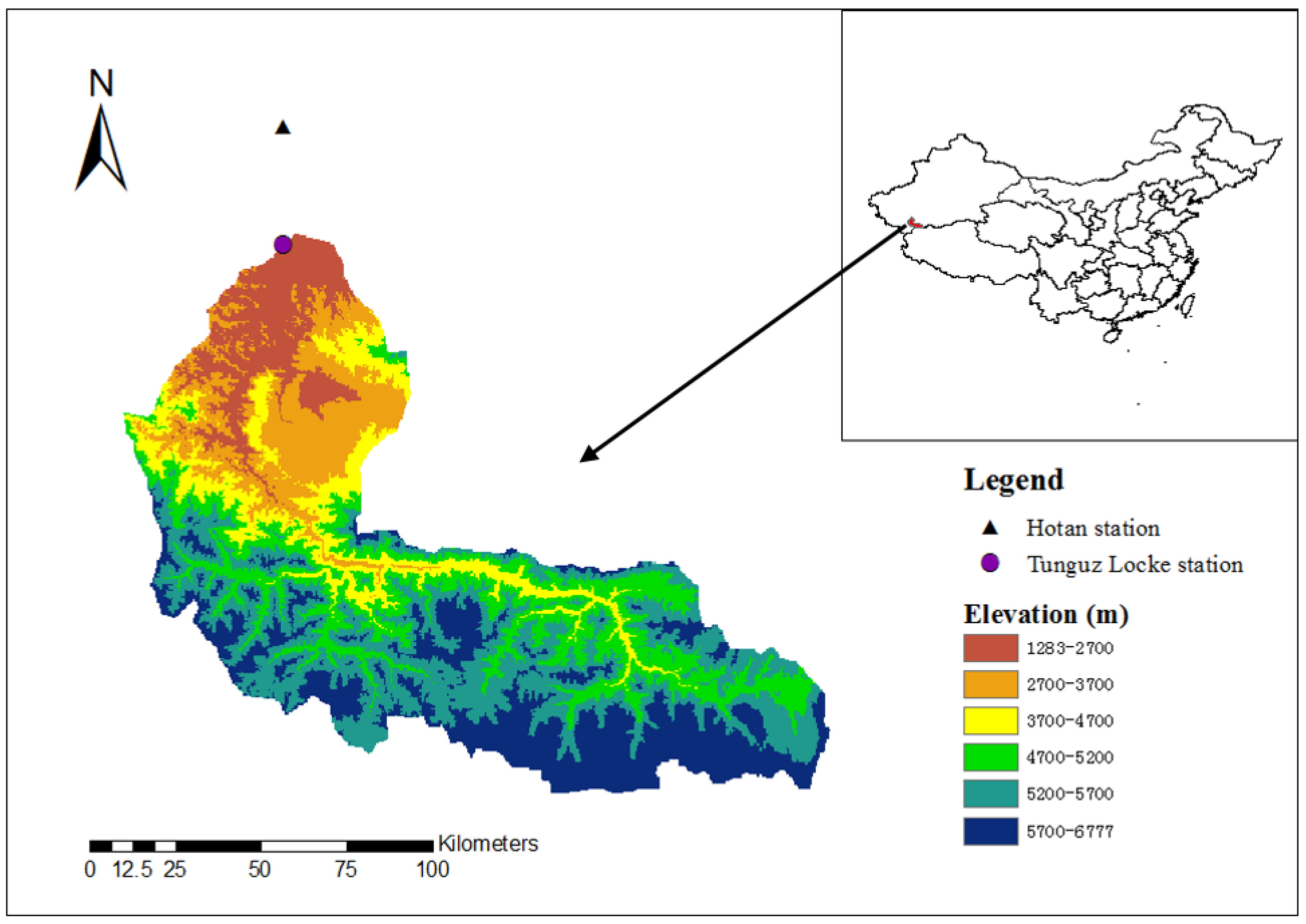
2.1. Study Area
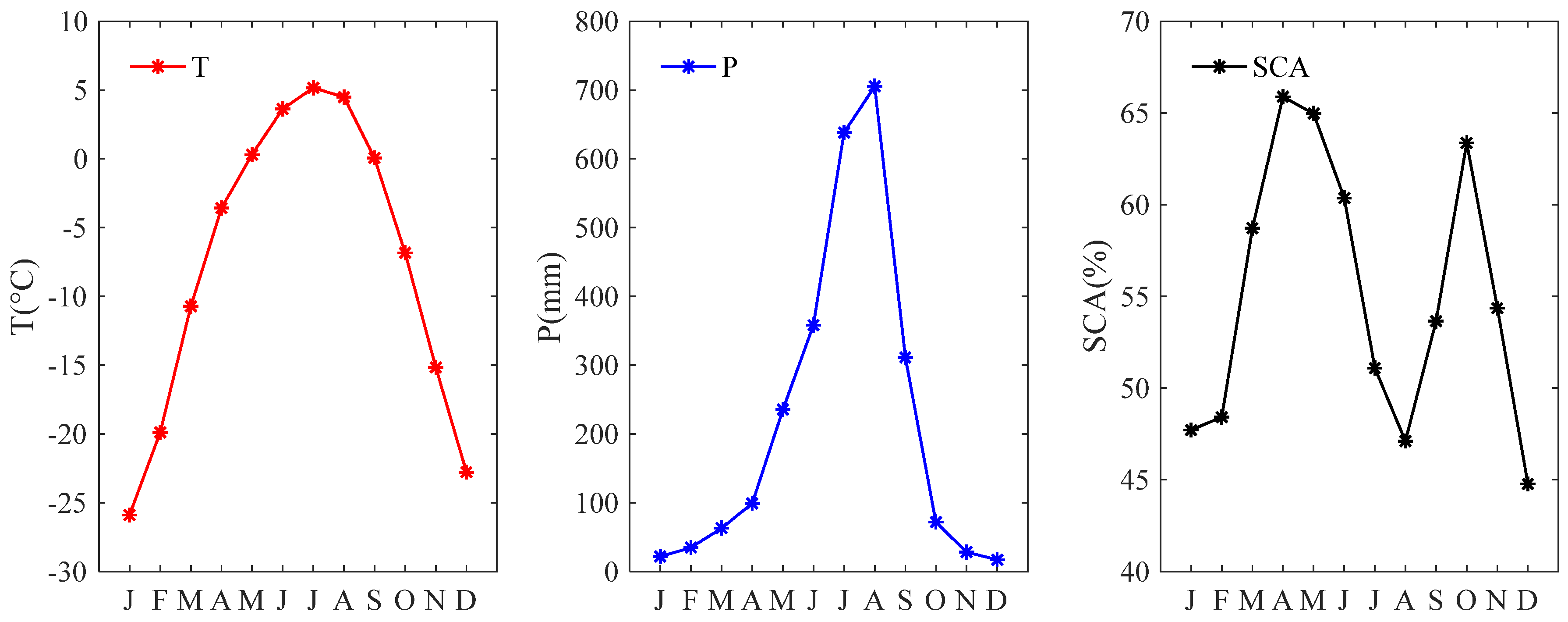
2.2. Data
3. Methods
3.1. SRM Modeling
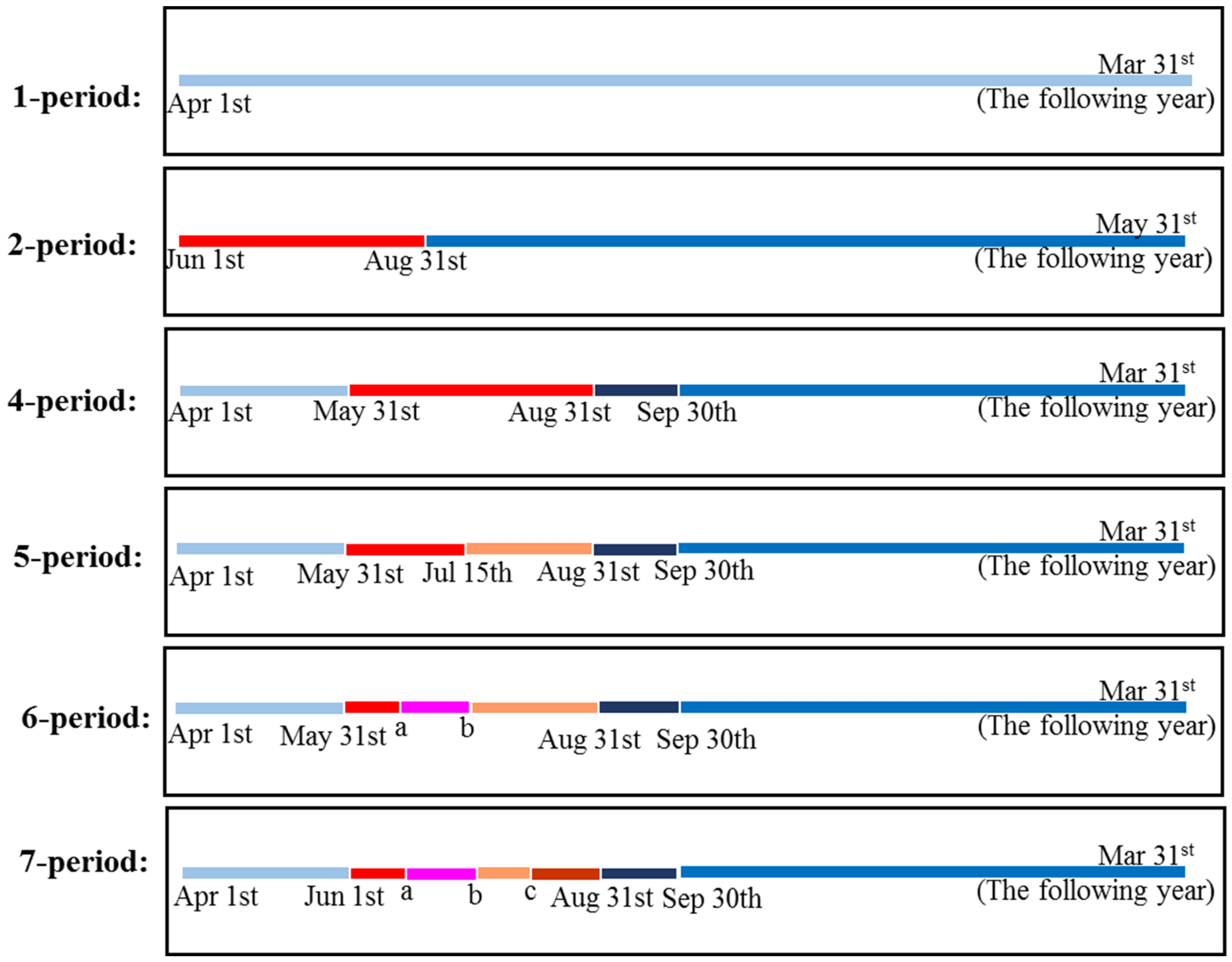
3.2. SRM Calibration Methods
3.3. Bias Correction of GCM Outputs
- The LOCI method was used to correct the precipitation occurrence, which ensures that the frequency of the precipitation occurrence simulated by GCMs at the reference period equals that of the observed data for a specific month. A threshold for precipitation occurrence determined at the historical period was then applied to the future period.
- The DT method was used to correct the empirical distribution of GCM-simulated precipitation and temperature magnitudes in terms of 100 quantiles from 0.01 to 1 with an interval of 0.01.
3.4. Future Snow Covered Area Projection
3.5. GLUE Method for Uncertainty Estimates
- 100,000 Monte Carlo sampling points of and were implemented from a feasible parameter space (0–1) with uniform distribution;
- The likelihood values were calculated for all 100,000 model runs;
- The likelihood functions (NSE and VE) and the threshold values (0.55 and ±10%, respectively) were specified as behavioral parameter sets; and
- Posterior parameter sets were extracted depending on the threshold of the likelihood functions.
4. Results
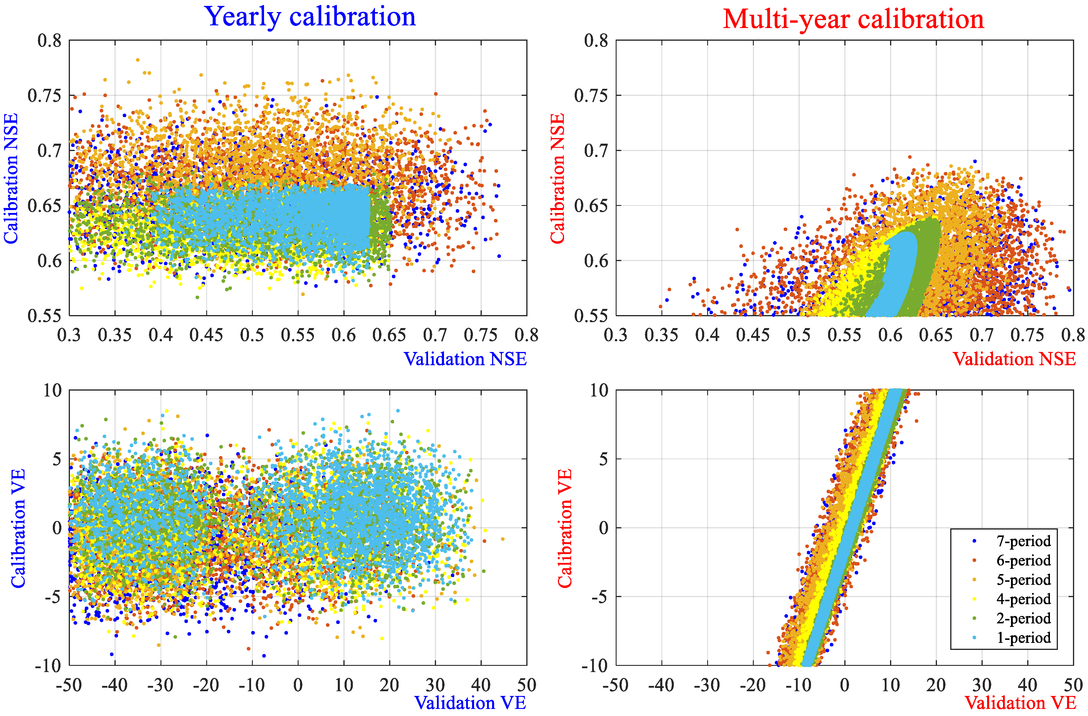
4.1. Parameter Uncertainty
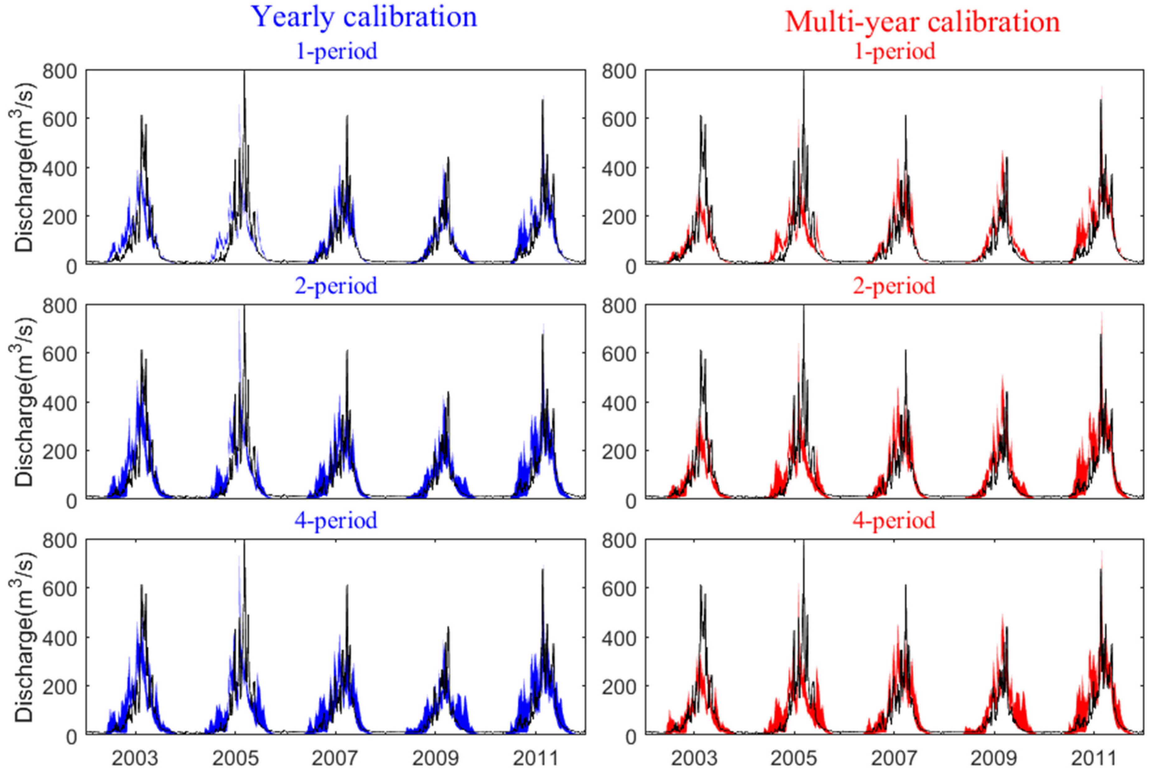
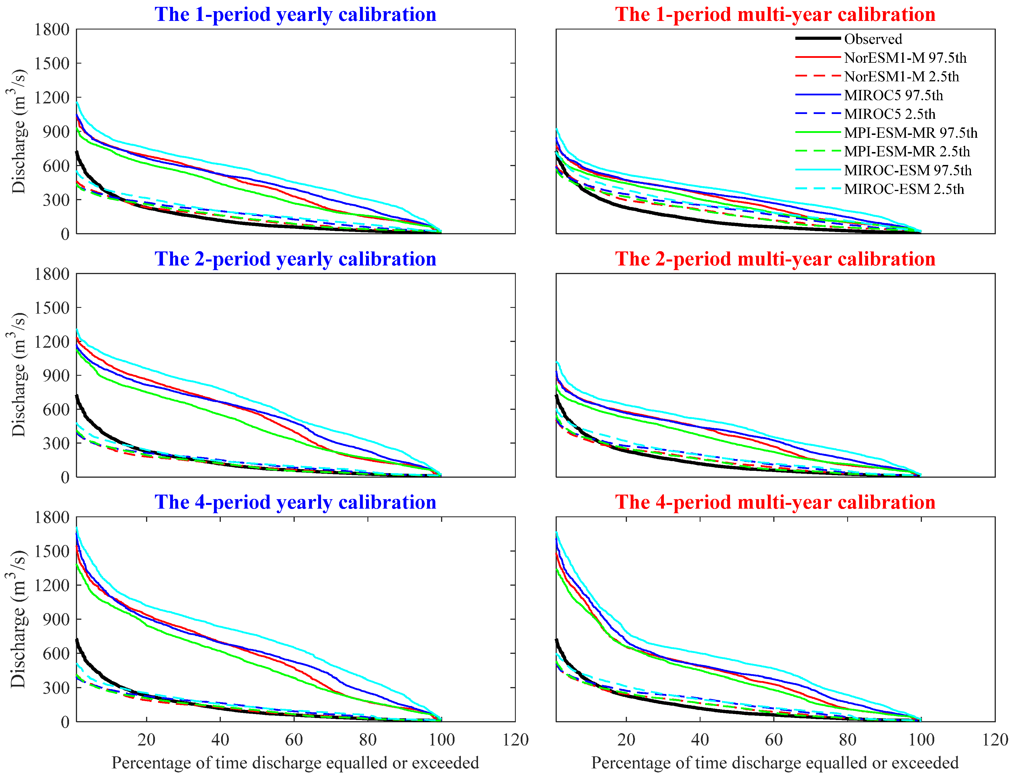
4.2. Confidence Interval of Discharge
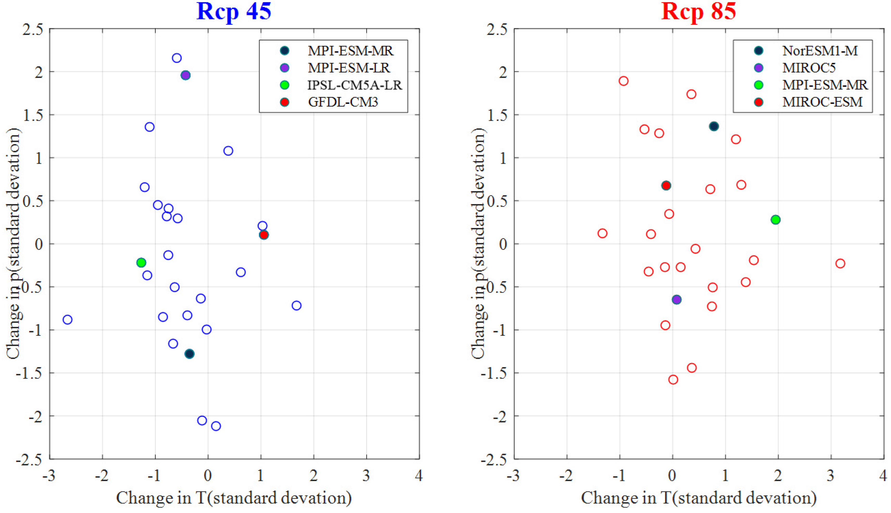
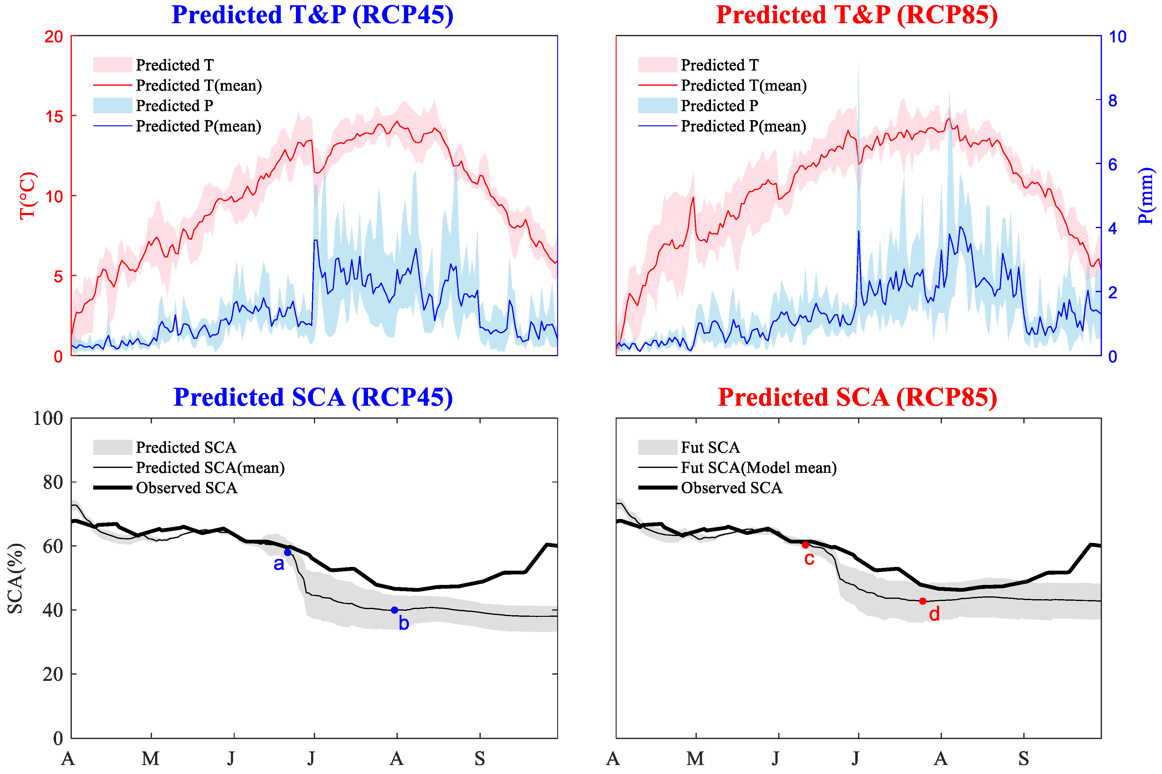
4.3. Projected Future Temperature, Precipitation, and SCA
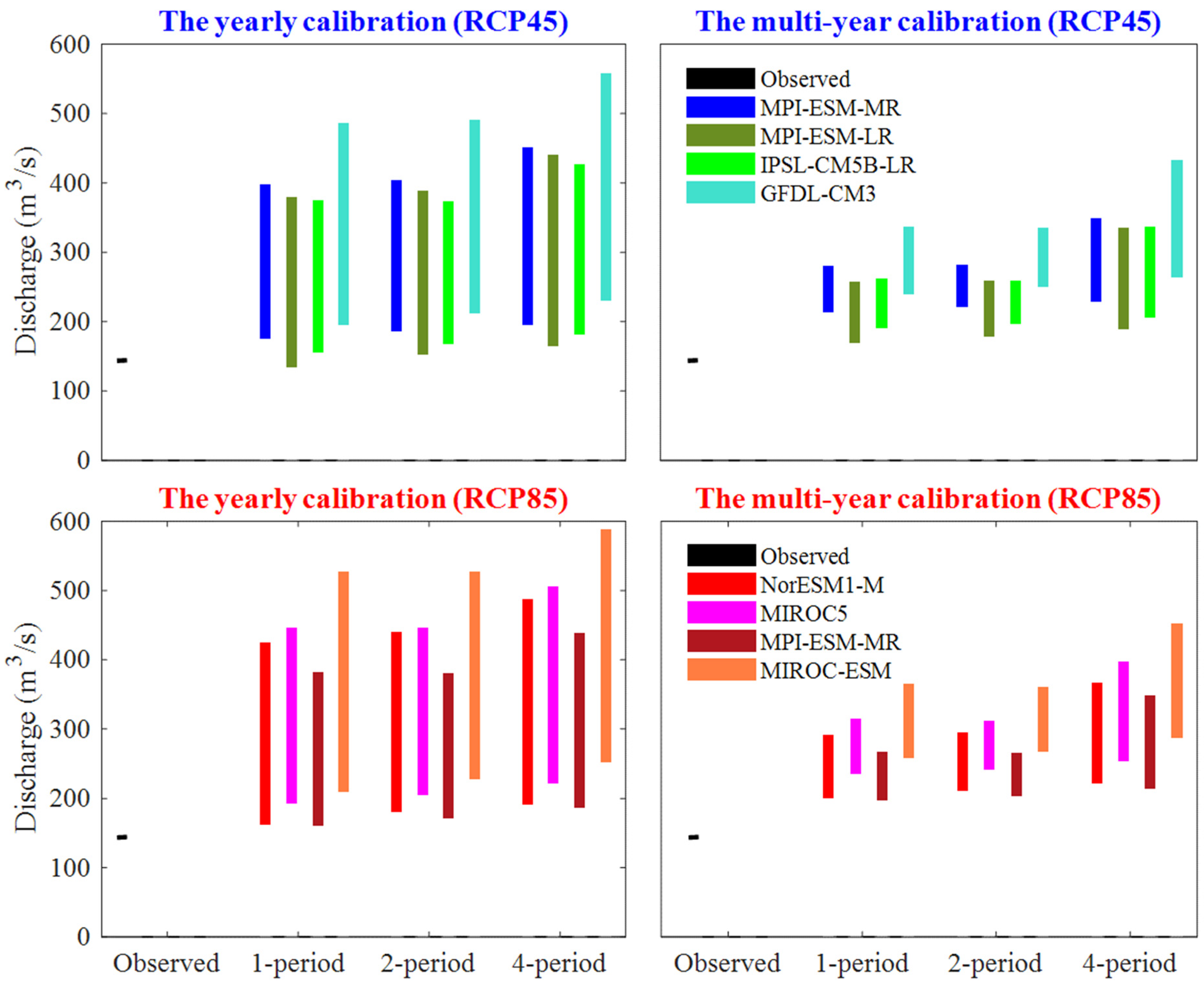
4.4. Uncertainty in the Discharge Projections
5. Discussion
6. Conclusions
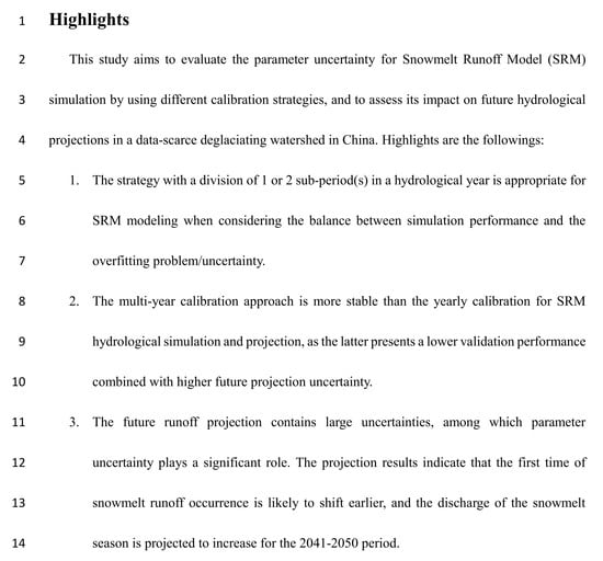
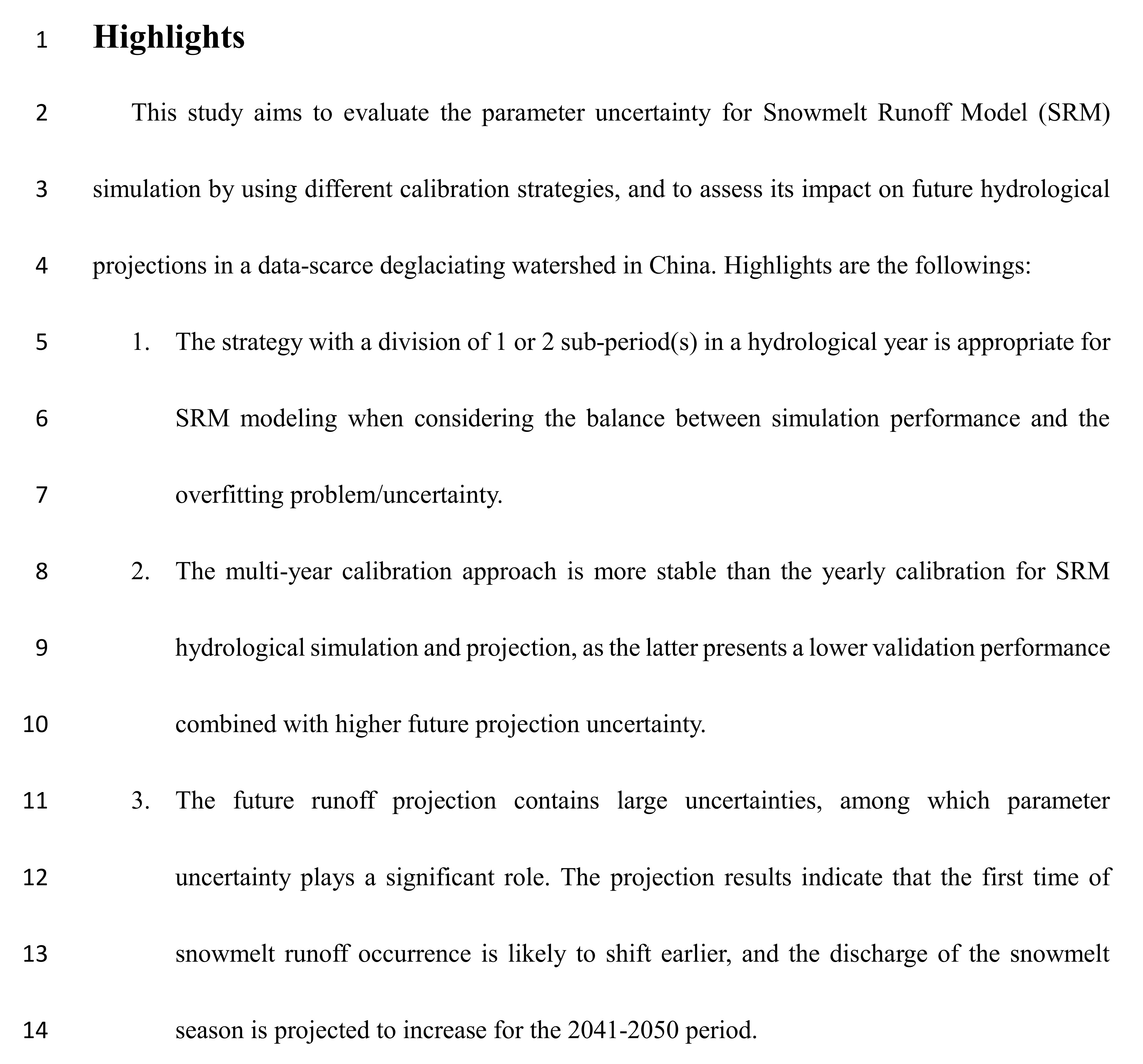
- The strategy with a division of 1 or 2 sub-period(s) in a hydrological year is appropriate for SRM modeling when considering the balance between simulation performance and the overfitting problem/uncertainty. In addition, the multi-year calibration approach is more stable than the yearly calibration for SRM hydrological simulation and projection, as the latter presents a lower validation performance combined with higher future projection uncertainty.
- The future runoff projection contains large uncertainties, among which parameter uncertainty plays a significant role. The projection results indicate that the onset of snowmelt runoff is likely to shift earlier, and the discharge of the snowmelt season is projected to increase for the 2041–2050 period.
Author Contributions
Funding
Acknowledgments
Conflicts of Interest
Appendix A
Appendix A.1. SRM Modelling
- = the average daily discharge (m3/s)
- /= the runoff coefficient expressing the losses as a ration of runoff to precipitation, with referring to snowmelt and referring to rainfall
- = the degree-day factor (cm/°C/day)
- = the number of degree-days (°C day)
- = the adjustment by temperature lapse rate when extrapolating the temperature from the station to the mean elevation of the zone (°C day)
- = the ratio of the snow covered area to the total area (%)
- = the precipitation contributing to runoff (cm), which is determined by a preselected threshold temperature, , to be rainfall or snowfall. The contribution of rainfall is immediate while snowfall will be kept on storage until melting conditions occur.
- = the area elevation zone (km2)
- = 10,000/86,400, the coefficient converting data from a runoff depth (cm×km2/day) to discharge (m3/s)
- = the recession coefficient,
- = the day number
Appendix A.1.1. Input Variables
Appendix A.1.2. Parameters
References
- Stocker, T.F.; Qin, D.; Plattner, G.-K.; Tignor, M.; Allen, S.K.; Boschung, J.; Nauels, A.; Xia, Y.; Bex, V.; Midgley, P.M. (Eds.) IPCC. Climate Change 2013: The Physical Science Basis. Contribution of Working Group I to the Fifth Assessment Report of the Intergovernmental Panel on Climate Change; Cambridge University Press: Cambridge, UK, 2013; p. 1535. [Google Scholar]
- Barnett, T.P.; Adam, J.C.; Lettenmaier, D.P. Potential impacts of a warming climate on water availability in snow-dominated regions. Nature. 2005, 438, 303. [Google Scholar] [CrossRef] [PubMed]
- Stewart, I.T. Changes in snowpack and snowmelt runoff for key mountain regions. Hydrol. Process. 2009, 23, 78–94. [Google Scholar] [CrossRef]
- Klein, I.M.; Rousseau, A.N.; Frigon, A.; Freudiger, D.; Gagnon, P. Evaluation of probable maximum snow accumulation: Development of a methodology for climate change studies. J. Hydrol. 2016, 537, 74–85. [Google Scholar] [CrossRef]
- Kudo, R.; Yoshida, T.; Masumoto, T. Uncertainty analysis of impacts of climate change on snow processes: Case study of interactions of GCM uncertainty and an impact model. J. Hydrol. 2017, 548, 196–207. [Google Scholar] [CrossRef]
- Hamlet, A.F.; Mote, P.W.; Clark, M.P.; Lettenmaier, D.P. Effects of Temperature and Precipitation Variability on Snowpack Trends in the Western United States*. J. Clim. 2005, 18, 4545–4561. [Google Scholar] [CrossRef]
- Khadka, D.; Babel, M.S.; Shrestha, S.; Tripathi, N.K. Climate change impact on glacier and snow melt and runoff in Tamakoshi basin in the Hindu Kush Himalayan (HKH) region. J. Hydrol. 2014, 511, 49–60. [Google Scholar] [CrossRef]
- Mukhopadhyay, B.; Khan, A. A reevaluation of the snowmelt and glacial melt in river flows within Upper Indus Basin and its significance in a changing climate. J. Hydrol. 2015, 527, 119–132. [Google Scholar] [CrossRef]
- Adam, J.C.; Hamlet, A.F.; Lettenmaier, D.P. Implications of global climate change for snowmelt hydrology in the twenty-first century. Hydrol. Process. 2009, 23, 962–972. [Google Scholar] [CrossRef]
- Vicuña, S.; Garreaud, R.D.; McPhee, J. Climate change impacts on the hydrology of a snowmelt driven basin in semiarid Chile. Clim. Chang. 2011, 105, 469–488. [Google Scholar] [CrossRef]
- Elias, E.H.; Rango, A.; Steele, C.M.; Mejia, J.F.; Smith, R. Assessing climate change impacts on water availability of snowmelt-dominated basins of the Upper Rio Grande basin. J. Hydrol. Reg. Stud. 2015, 3, 525–546. [Google Scholar] [CrossRef]
- Quick, M.; Pipes, A. Daily and seasonal runoff forecasting with a water budget model. In Role of Snow and Ice in Hydrology Proceedings of the UNESCO/WMO/IAHS Symposium; World Meteorological Organization: Banff, AB, Canada, 1972; pp. 1017–1034. [Google Scholar]
- Leavesley, G.H.; Lichty, R.W.; Troutman, B.M.; Saindon, L.G. Precipitation-runoff modeling system: User’s manual. Geol. Surv. Water Ivestig. 1983, 83–4238. [Google Scholar]
- Jordan, R. A One-Dimensional Temperature Model for a Snow Cover: Technical Documentation for SNTHERM. 89; Cold Regions Research and Engineering Lab Hanover NH: Washington, DC, USA, 1991. [Google Scholar]
- Bergstrom, S.; Forsman, A. Development of a conceptual deterministic rainfall-runoff model. Nord. Hydrol. 1973, 4, 147–170. [Google Scholar] [CrossRef]
- Martinec, J. Snowmelt-Runoff Model for Stream Flow Forecasts. Nord. Hydrol. 1975, 6, 145–154. [Google Scholar] [CrossRef]
- Charrois, L.; Cosme, E.; Dumont, M.; Lafaysse, M.; Picard, G. On the assimilation of optical reflectances and snow depth observations into a detailed snowpack model. Cryosphere 2016, 10, 1021–1038. [Google Scholar] [CrossRef]
- Magnusson, J.; Gustafsson, D.; Hüsler, F.; Jonas, T. Assimilation of point swe data into a distributed snow cover model comparing two contrasting methods. Water Resour. Res. 2014, 50, 7816–7835. [Google Scholar] [CrossRef]
- Magnusson, J.; Winstral, A.; Stordal, A.S.; Essery, R.; Jonas, T. Improving physically based snow simulations by assimilating snow depths using the particle filter. Water Resour. Res. 2017, 53, 1125–1143. [Google Scholar] [CrossRef]
- USDA-NRCS. National Engineering Handbook: Part 630—Hydrology; USDA Soil Conservation Service: Washington, DC, USA, 2004.
- Hock, R. Temperature index melt modeling in mountain areas. J. Hydrol. 2003, 282, 104–115. [Google Scholar] [CrossRef]
- Seidel, K.; Martinec, J.; Baumgartner, M.F. Modeling runoff and impact of climate change in large himalayan basins. In Proceedings of the International Conference on Integrated Water Resources Management (ICIWRM), Roorke, India, 19–21 December 2000. [Google Scholar]
- Nazari, M.A.; Saleh, F.N.; Chavoshian, S.A. Flood forecasting and river flow modeling in mountainous basin with significant contribution of snowmelt runoff. Presented at the International Conference on Flood Management, Tsukuba, Japan, 25 September 2011. [Google Scholar]
- Ye, L.; Zhou, J.; Zeng, X.; Guo, J.; Zhang, X. Multi-objective optimization for construction of prediction interval of hydrological models based on ensemble simulations. J. Hydrol. 2014, 519, 925–933. [Google Scholar] [CrossRef]
- Tahir, A.A.; Hakeem, S.A.; Hu, T.; Hayat, H.; Yasir, M. Simulation of snowmelt-runoff under climate change scenarios in a data-scarce mountain environment. Int. J. Digit. Earth 2017, 1–21. [Google Scholar] [CrossRef]
- Xie, S.; Du, J.; Zhou, X.; Zhang, X.; Feng, X.; Zheng, W.; Xu, C.-Y. A progressive segmented optimization algorithm for calibrating time-variant parameters of the snowmelt runoff model (SRM). J. Hydrol. 2018, 566, 470–483. [Google Scholar] [CrossRef]
- Refsgaard, J.C.; Storm, B. Construction, Calibration and Validation of Hydrological Models. Distrib. Hydrol. Model. 1990, 22, 41–54. [Google Scholar] [CrossRef]
- Wilby, R.L. Uncertainty in water resource model parameters used for climate change impact assessment. Hydrol. Process. 2005, 19, 3201–3219. [Google Scholar] [CrossRef]
- Vrugt, J.A.; Gupta, H.V.; Bouten, W.; Sorooshian, S. A Shuffled Complex Evolution Metropolis algorithm for optimization and uncertainty assessment of hydrologic model parameters. Water Resour. Res. 2003, 39. [Google Scholar] [CrossRef]
- Finger, D.; Vis, M.; Huss, M.; Seibert, J. The value of multiple data set calibration versus model complexity for improving the performance of hydrological models in mountain catchments. Water Resour. Res. 2015, 51, 1939–1958. [Google Scholar] [CrossRef]
- Bastola, S.; Murphy, C.; Sweeney, J. The role of hydrological modeling uncertainties in climate change impact assessments of Irish river catchments. Adv. Water Resour. 2011, 34, 562–576. [Google Scholar] [CrossRef]
- Brigode, P.; Oudin, L.; Perrin, C. Hydrological model parameter instability: A source of additional uncertainty in estimating the hydrological impacts of climate change? J. Hydrol. 2013, 476, 410–425. [Google Scholar] [CrossRef]
- Joseph, J.; Ghosh, S.; Pathak, A.; Sahai, A.K. Hydrologic impacts of climate change: Comparisons between hydrological parameter uncertainty and climate model uncertainty. J. Hydrol. 2018, 566, 1–22. [Google Scholar] [CrossRef]
- Jin, X.; Xu, C.-Y.; Zhang, Q.; Singh, V.P. Parameter and modeling uncertainty simulated by GLUE and a formal Bayesian method for a conceptual hydrological model. J. Hydrol. 2010, 383, 147–155. [Google Scholar] [CrossRef]
- Li, L.; Xu, C.-Y.; Xia, J.; Engeland, K.; Reggiani, P. Uncertainty estimates by Bayesian method with likelihood of AR (1) plus Normal model and AR (1) plus Multi-Normal model in different time-scales hydrological models. J. Hydrol. 2011, 406, 54–65. [Google Scholar] [CrossRef]
- Raje, D.; Krishnan, R. Bayesian parameter uncertainty modeling in a macroscale hydrologic model and its impact on Indian river basin hydrology under climate change. Water Resour. Res. 2012, 48. [Google Scholar] [CrossRef]
- Beven, K.; Binley, A. The future of distributed models: Model calibration and uncertainty prediction. Hydrol. Process. 1992, 6, 279–298. [Google Scholar] [CrossRef]
- Saltelli, A.; Annoni, P. Sensitivity Analysis; Wiley: Hoboken, NJ, USA, 2000. [Google Scholar]
- Blasone, R.S.; Madsen, H.; Rosbjerg, D. Uncertainty assessment of integrated distributed hydrological models using glue with markov chain monte carlo sampling. J. Hydrol. 2008, 353, 18–32. [Google Scholar] [CrossRef] [Green Version]
- Li, L.; Xia, J.; Xu, C.-Y.; Singh, V.P. Evaluation of the subjective factors of the GLUE method and comparison with the formal Bayesian method in uncertainty assessment of hydrological models. J. Hydrol. 2010, 390, 210–221. [Google Scholar] [CrossRef]
- Fuentes-Andino, D.; Beven, K.; Halldin, S.; Xu, C.-Y.; Baldassarre, G.D. Reproducing an extreme flood with uncertain post–event information. J. Hydrol. Earth Syst. Sci. 2017, 21, 3597–3618. [Google Scholar] [CrossRef] [Green Version]
- Metropolis, N.; Ulam, S. The Monte Carlo Method. J. Am. Stat. Assoc. 1949, 44, 335–341. [Google Scholar] [CrossRef]
- Blasone, R.-S.; Vrugt, J.A.; Madsen, H.; Rosbjerg, D.; Robinson, B.A.; Zyvoloski, G.A. Generalized likelihood uncertainty estimation (GLUE) using adaptive Markov Chain Monte Carlo sampling. Adv. Water Resour. 2008, 31, 630–648. [Google Scholar] [CrossRef] [Green Version]
- Prasad, V.H.; Roy, P.S. Estimation of Snowmelt Runoff in Beas Basin, India. Geocarto Int. 2005, 20, 41–47. [Google Scholar] [CrossRef]
- Li, X.; Williams, M.W. Snowmelt runoff modeling in an arid mountain watershed, Tarim Basin, China. Hydrol. Process. 2008, 22, 3931–3940. [Google Scholar] [CrossRef]
- Abudu, S.; Cui, C.L.; Saydi, M.; King, J.P. Application of snowmelt runoff model (SRM) in mountainous watersheds: A review. Water Sci. Eng. 2012, 5, 123–136. [Google Scholar]
- Martinec, J.; Rango, A.; Major, E. The Snowmelt-Runoff Model (S.R.M.) User’s Manual; NASA Reference Publication 1100: Washington, DC, USA, 1983. [Google Scholar]
- Senzeba, K.T.; Rajkumari, S.; Bhadra, A.; Bandyopadhyay, A. Response of streamflow to projected climate change scenarios in an eastern Himalayan catchment of India. J. Earth Syst. Sci. 2016, 125, 443–457. [Google Scholar] [CrossRef] [Green Version]
- Zhang, G.; Xie, H.; Yao, T.; Li, H.; Duan, S. Quantitative water resources assessment of Qinghai Lake basin using Snowmelt Runoff Model (SRM). J. Hydrol. 2014, 519, 976–987. [Google Scholar] [CrossRef]
- Fuladipanah, M.; Jorabloo, M. The estimation of snowmelt runoff using SRM case study (Gharasoo basin, Iran). World Appl. Sci. J. 2012, 17, 433–438. [Google Scholar]
- Farr, T.G.; Rosen, P.A.; Caro, E.; Crippen, R.; Duren, R.; Hensley, S.; Alsdorf, D. The Shuttle Radar Topography Mission. Rev. Geophys. 2007, 45. [Google Scholar] [CrossRef] [Green Version]
- Available online: http://data.cma.cn (accessed on 10 November 2019).
- Andrew, T.; Roddy, H.; Richard, T.; Zheng, X.G. Thin plate smoothing spline interpolation of daily rainfall for New Zealand using a climatological rainfall surface. Int. J. Climatol. 2006, 26, 2097–2115. [Google Scholar]
- Zhao, Y.F.; Zhu, J. Assessing quality of grid daily precipitation datasets in china in recent 50 years. Plateau Meteorol. 2015, 34, 50–58. [Google Scholar]
- Available online: http://nsidc.org/data (accessed on 10 November 2019).
- Huang, X.; Zhang, X.; Li, X.; Liang, T. Accuracy analysis for MODIS snow products of MOD10A1 and MOD10A2 in northern Xinjiang area. J. Glaciol. Geocryol. 2007, 29, 722–729. [Google Scholar]
- Taylor, K.E.; Stouffer, R.J.; Meehl, G.A. An overview of CMIP5 and the experiment design. Bull. Am. Meteorol. Soc. 2012, 93, 485–498. [Google Scholar] [CrossRef] [Green Version]
- Hartigan, J.A.; Wong, M.A. Algorithm AS 136: A k-means clustering algorithm. J. R. Stat. Soc. Ser. C (Appl. Stat.) 1979, 28, 100–108. [Google Scholar] [CrossRef]
- Cannon, A.J. Selecting GCM Scenarios that Span the Range of Changes in a Multimodel Ensemble: Application to CMIP5 Climate Extremes Indices*. J. Clim. 2015, 28, 1260–1267. [Google Scholar] [CrossRef]
- Chen, J.; Brissette, F.P.; Lucas-Picher, P. Transferability of optimally-selected climate models in the quantification of climate change impacts on hydrology. Clim. Dyn. 2016, 47, 3359–3372. [Google Scholar] [CrossRef]
- Wang, H.M.; Chen, J.; Cannon, A.J.; Xu, C.Y.; Chen, H. Transferability of climate simulation uncertainty to hydrological impacts. Hydrol. Earth Syst. Sci. 2018, 22, 3739–3759. [Google Scholar] [CrossRef] [Green Version]
- Martinec, J.; Rango, A.; Roberts, R.T. Snowmelt Runoff Model (SRM) User’s Manual; New Mexico State University Press: New Mexico, NM, USA, 2008; pp. 19–39. [Google Scholar]
- Nash, J.E.; Sutcliffe, J.V. River flow forecasting through conceptual models part I—A discussion of principles. J. Hydrol. 1970, 10, 282–290. [Google Scholar] [CrossRef]
- Chen, J.; Brissette, F.P.; Poulin, A.; Leconte, R. Overall uncertainty study of the hydrological impacts of climate change for a Canadian watershed. Water Resour. Res. 2011, 47. [Google Scholar] [CrossRef]
- Liu, J.; Zhu, A.-X.; Duan, Z. Evaluation of trmm 3b42 precipitation product using rain gauge data in Meichuan watershed, Poyang Lake Basin, China. J. Resour. Ecol. 2012, 3, 359–366. [Google Scholar]
- Bartier, P.M.; Keller, C.P. Multivariate interpolation to incorporate thematic surface data using inverse distance weighting (idw). Comput. Geosci. 1996, 22, 795–799. [Google Scholar] [CrossRef]
- Chen, J.; Brissette, F.P.; Chaumont, D.; Braun, M. Performance and uncertainty evaluation of empirical downscaling methods in quantifying the climate change impacts on hydrology over two North American river basins. J. Hydrol. 2013, 479, 200–214. [Google Scholar] [CrossRef]
- Schmidli, J.; Frei, C.; Vidale, P.L. Downscaling from GCM precipitation: A benchmark for dynamical and statistical downscaling methods. Int. J. Climatol. 2006, 26, 679–689. [Google Scholar] [CrossRef]
- Mpelasoka, F.S.; Chiew, F.H.S. Influence of Rainfall Scenario Construction Methods on Runoff Projections. J. Hydrometeorol. 2009, 10, 1168–1183. [Google Scholar] [CrossRef]
- Rango, A.; Martinec, J. Areal extent of seasonal snow cover in a changed climate. Hydrol. Res. 1994, 25, 233–246. [Google Scholar] [CrossRef]
- Ratto, M.; Tarantola, S.; Saltelli, A. Sensitivity analysis in model calibration: GSA-GLUE approach. Comput. Phys. Commun. 2001, 136, 212–224. [Google Scholar] [CrossRef]
- Li, L.; Xia, J.; Xu, C.Y.; Chu, J.J.; Wang, R.; Cluckie, I.D.; Mynett, A. Analyse the sources of equifinality in hydrological model using GLUE methodology. Paper presented at the Hydroinformatics in Hydrology, Hydrogeology and Water Resources. In Proceedings of the Symposium JS.4 at the Joint IAHS IAH Convention, Hyderabad, India, 6–12 September 2009. [Google Scholar]
- Katwijk, V.F.; Rango, A.; Childress, A.E. Effect of Simulated Climate Change on Snowmelt Runoff Modeling in Selected Basins. J. Am. Water Resour. Assoc. 1993, 29, 755–766. [Google Scholar] [CrossRef]
- Matott, L.S.; Babendreier, J.E.; Purucker, S.T. Evaluating uncertainty in integrated environmental models: A review of concepts and tools. Water Resour. Res. 2009, 45. [Google Scholar] [CrossRef] [Green Version]
- Butts, M.B.; Payne, J.T.; Kristensen, M.; Madsen, H. An evaluation of the impact of model structure on hydrological modeling uncertainty for streamflow simulation. J. Hydrol. 2004, 298, 242–266. [Google Scholar] [CrossRef]
- Jakeman, A.J.; Hornberger, G.M. How much complexity is warranted in a rainfall-runoff model? Water Resour. Res. 1993, 29, 2637–2649. [Google Scholar] [CrossRef]
- Seiller, G.; Roy, R.; Anctil, F. Influence of three common calibration metrics on the diagnosis of climate change impacts on water resources. J. Hydrol. 2017, 547, 280–295. [Google Scholar] [CrossRef]
- Wang, J.; Li, H.; Hao, X. Responses of snowmelt runoff to climatic change in an inland river basin, Northwestern China, over the past 50 years. Hydrol. Earth Syst. Sci. 2010, 14, 1979–1987. [Google Scholar] [CrossRef] [Green Version]
- Tian, Y.; Xu, Y.P.; Booij, M.J.; Wang, G. Uncertainty in future high flows in Qiantang river basin, China. J. Hydrometeorol. 2015, 16, 363–380. [Google Scholar] [CrossRef] [Green Version]
- Wilby, R.L.; Harris, I. A framework for assessing uncertainties in climate change impacts: Low-flow scenarios for the River Thames, UK. Water Resour. Res. 2006, 42. [Google Scholar] [CrossRef]
- Stedinger, J.R.; Vogel, R.M.; Lee, S.U.; Batchelder, R. Appraisal of the generalized likelihood uncertainty estimation (GLUE) method. Water Resour. Res. 2008, 44. [Google Scholar] [CrossRef]
- Li, Z.; Shao, Q.; Xu, Z.; Cai, X. Analysis of parameter uncertainty in semi-distributed hydrological models using bootstrap method: A case study of SWAT model applied to Yingluoxia watershed in northwest China. J. Hydrol. 2010, 385, 76–83. [Google Scholar] [CrossRef]
- Ruelland, D.; Hublart, P.; Tramblay, Y. Assessing uncertainties in climate change impacts on runoff in Western Mediterranean basins. Proc. Int. Assoc. Hydrol. Sci. 2015, 371, 75–81. [Google Scholar] [CrossRef] [Green Version]
- Vaze, J.; Post, D.A.; Chiew, F.H.S.; Perraud, J.M.; Viney, N.R.; Teng, J. Climate non-stationarity—Validity of calibrated rainfall–runoff models for use in climate change studies. J. Hydrol. 2010, 394, 447–457. [Google Scholar] [CrossRef]
- Van den Broeke, M.R.; Smeets, C.J.P.P.; van de Wal, R.S.W. The seasonal cycle and interannual variability of surface energybalance and melt in the ablation zone of the west Greenland ice sheet. Cryosphere 2011, 5, 377–390. [Google Scholar] [CrossRef] [Green Version]
- Bougamont, M.; Hunke, E.; Tulaczyk, S. Sensitivity of ocean circulation and sea-ice conditions to loss of west antarctic ice shelves and ice sheet. J. Glaciol. 2007, 53, 490–498. [Google Scholar] [CrossRef] [Green Version]
- Huss, M.; Farinotti, D.; Bauder, A.; Funk, M. Moddelling runoff from highly glacierized alpine drainage basins in a changing climate. Hydrol. Process. 2008, 22, 3888–3902. [Google Scholar] [CrossRef]
- Zhang, Y.; Liu, S.; Ding, Y. Observed degree-day factors and their spatial variation on glaciers in western China. Ann. Glaciol. 2006, 43, 301–306. [Google Scholar] [CrossRef] [Green Version]


| Zone | Elevation Range (m) | Mean Elevation (m) | Area (km2) | Area (%) |
|---|---|---|---|---|
| A | 1280–2700 | 2230 | 1324 | 9.07 |
| B | 2701–3700 | 3190 | 2248 | 15.40 |
| C | 3701–4700 | 4250 | 2170 | 14.86 |
| D | 4701–5200 | 4975 | 2485 | 17.02 |
| E | 5201–5700 | 5440 | 3238 | 22.18 |
| F | 5701–6780 | 6020 | 3135 | 21.47 |
| Total | 1280–6780 | 4470 | 14600 | 100 |
| Model Name | Institute/Country | Horizontal Resolution (lon×lat) |
|---|---|---|
| MPI-ESM-MR | Max Planck Institute for Meteorology, Germany | 192 × 96 |
| MPI-ESM-LR | Max Planck Institute for Meteorology, Germany | 192 × 96 |
| IPSL-CM5A-LR | Institute Pierre-Simon Laplace, France | 96 × 96 |
| GFDL-CM3 | USA | 144 × 90 |
| NorESM1-M | Norwegian Climate Centre, Norway | 144 × 96 |
| MIROC5 | MIROC, Japan | 256 × 128 |
| MIROC-ESM | MIROC, Japan | 128 × 64 |
| Model Parameters | Values |
|---|---|
| Degree Day Factor (cm/°C/day) | 0.3 |
| Lapse Rate (°C/100 m) | 0.65 |
| Threshold Temperature, | 1 (June–August); 3 (September–May) |
| Rainfall Contributing Area, RCA | 1 (May–September); 0 (October–April) |
| Recession Coefficient, K, which is Determined by: | ; |
| Sub-Period(s) | Yearly Calibration | Multi-Year Calibration | ||||
|---|---|---|---|---|---|---|
| ARIL | PCI | PUCI | ARIL | PCI | PUCI | |
| 1 | 0.454 | 0.204 | 0.559 | 0.440 | 0.178 | 0.517 |
| 2 | 1.009 | 0.430 | 0.475 | 0.848 | 0.376 | 0.501 |
| 4 | 1.287 | 0.500 | 0.427 | 1.192 | 0.470 | 0.436 |
| 5 | 1.531 | 0.586 | 0.416 | 1.361 | 0.538 | 0.432 |
| 6 | 1.546 | 0.596 | 0.418 | 1.356 | 0.556 | 0.447 |
| 7 | 1.548 | 0.606 | 0.424 | 1.396 | 0.570 | 0.444 |
© 2019 by the authors. Licensee MDPI, Basel, Switzerland. This article is an open access article distributed under the terms and conditions of the Creative Commons Attribution (CC BY) license (http://creativecommons.org/licenses/by/4.0/).
Share and Cite
Xiang, Y.; Li, L.; Chen, J.; Xu, C.-Y.; Xia, J.; Chen, H.; Liu, J. Parameter Uncertainty of a Snowmelt Runoff Model and Its Impact on Future Projections of Snowmelt Runoff in a Data-Scarce Deglaciating River Basin. Water 2019, 11, 2417. https://doi.org/10.3390/w11112417
Xiang Y, Li L, Chen J, Xu C-Y, Xia J, Chen H, Liu J. Parameter Uncertainty of a Snowmelt Runoff Model and Its Impact on Future Projections of Snowmelt Runoff in a Data-Scarce Deglaciating River Basin. Water. 2019; 11(11):2417. https://doi.org/10.3390/w11112417
Chicago/Turabian StyleXiang, Yiheng, Lu Li, Jie Chen, Chong-Yu Xu, Jun Xia, Hua Chen, and Jie Liu. 2019. "Parameter Uncertainty of a Snowmelt Runoff Model and Its Impact on Future Projections of Snowmelt Runoff in a Data-Scarce Deglaciating River Basin" Water 11, no. 11: 2417. https://doi.org/10.3390/w11112417