Space–Time Kriging of Precipitation: Modeling the Large-Scale Variation with Model GAMLSS
by
 , , and
Elias Silva de Medeiros
1,* ,
,
Renato Ribeiro de Lima
2, 
Ricardo Alves de Olinda
3,
Leydson G. Dantas
4 and
Carlos Antonio Costa dos Santos
4,5 1
FACET, Federal University of Grande Dourados, Dourados 79.825-070, Brazil
2
Department of Statistics, Federal University of Lavras, Lavras 37.200-000, Brazil
3
Department of Statistics, Paraíba State University, Campina Grande-PB 58.429-500, Brazil
4
Academic Unity of Atmospheric Sciences, Center for Technology and Natural Resources, Federal University of Campina Grande-PB, Campina Grande 58.109-970, Brazil
5
Daugherty Water for Food Global Institute, University of Nebraska, Lincoln, NE 68588-6203, USA
*
Author to whom correspondence should be addressed.
Water 2019, 11(11), 2368; https://doi.org/10.3390/w11112368
Submission received: 16 October 2019
/
Revised: 1 November 2019
/
Accepted: 7 November 2019
/
Published: 12 November 2019
(This article belongs to the Special Issue Assessment of Spatial and Temporal Variability of Water Resources)
Abstract
:Knowing the dynamics of spatial–temporal precipitation distribution is of vital significance for the management of water resources, in highlight, in the northeast region of Brazil (NEB). Several models of large-scale precipitation variability are based on the normal distribution, not taking into consideration the excess of null observations that are prevalent in the daily or even monthly precipitation information of the region under study. This research proposes a novel way of modeling the trend component by using an inflated gamma distribution of zeros. The residuals of this regression are generally space–time dependent and have been modeled by a space–time covariance function. The findings show that the new techniques have provided reliable and precise precipitation estimates, exceeding the techniques used previously. The modeling provided estimates of precipitation in nonsampled locations and unobserved periods, thus serving as a tool to assist the government in improving water management, anticipating society’s needs and preventing water crises.
1. Introduction
An effort has emerged in several areas of knowledge, especially in the climate sciences, to analyze a phenomenon by both space and time [1,2,3]. It is already established that the spatial–temporal behavior of rainfall is of great importance for the water resources of a region and that it has a direct influence on human activities, such as agriculture and commerce [4].
The northeast region of Brazil (NEB) is characterized by irregular distributions of rainfall, resulting in high spatial and temporal variability of precipitation [4]. In this region, it is common to observe high rainfall indices in a particular location and no record of rain in its surroundings [5]. The state of Paraíba, located in this region, presents the same characteristics, with periods of drought in rainy seasons and behavior different from the precipitation between the mesoregions that constitute the region [6]. Consequently, Paraíba presents a problem concerning the spatiotemporal variability of rainfall. The high variability of recorded rainfall in this region may be attributed to the characteristics of the meteorological systems and their dates of installation in different regions of the state. The periodicity is related to the general behavior of sea surface temperature (SST) in the tropical Pacific region, contributing to the events of El Niño and La Niña, and most notably, by the behavior of the SST in the tropical Atlantic region due to its proximity to the study area. In the literature, several studies have evaluated precipitation in this region using spatial statistics techniques [7,8]. However, these previous works did not take spatial and temporal dependence into account simultaneously.
Several previous works used multiple linear regression to model the deterministic component, such as the Gaussian model [9,10,11]. These works assumed that the variable response to be studied presented a behavior that could be correctly modeled by a Gaussian approach.
However, recent studies have evaluated non-Gaussian models, including generalized linear models (GLM), with variable response Gamma [12,13]. Once the Gamma model is assumed, the variable domain has to be strictly positive, and it does not include the value zero. For example, Menezes et al. (2016) [12] and Monteiro et al. (2017) [13] analyzed the concentration of NO2, which had asymmetric behavior with excesses of zero. However, when using GLM with Gamma distribution, it is not possible to model the frequency of zeroes in the variable under study. To circumvent this limitation, some models captured the frequency of zeroes in continuous variables. Stauffer et al. (2017) [3] analyzed the spatial–temporal distribution of daily precipitation at 117 stations located in Tirol, Austria, over 42 years. These authors pointed to the high frequency of zero observations in the data, suggesting the use of the normal zero-censored model. However, only the trend component was modeled, not taking into account the spatial–temporal dependence of precipitation in this region.
In this study, we analyzed the total monthly rainfall measured in the State of Paraíba, Brazil, which presents an asymmetrical behavior and has a high incidence of zeros, which is a climate characteristic of the region under study. Thus, to model this behavior, a new approach in the regression adjustment is proposed by applying generalized additive models for location, scale, and shape (GAMLSS) [14]. These models have several advantages, such as all distribution parameters can be modeled as covariate functions, cases of over-dispersion and excess of zeroes in the data can be modeled, and any distribution to the response variable can be adjusted.
2. Materials
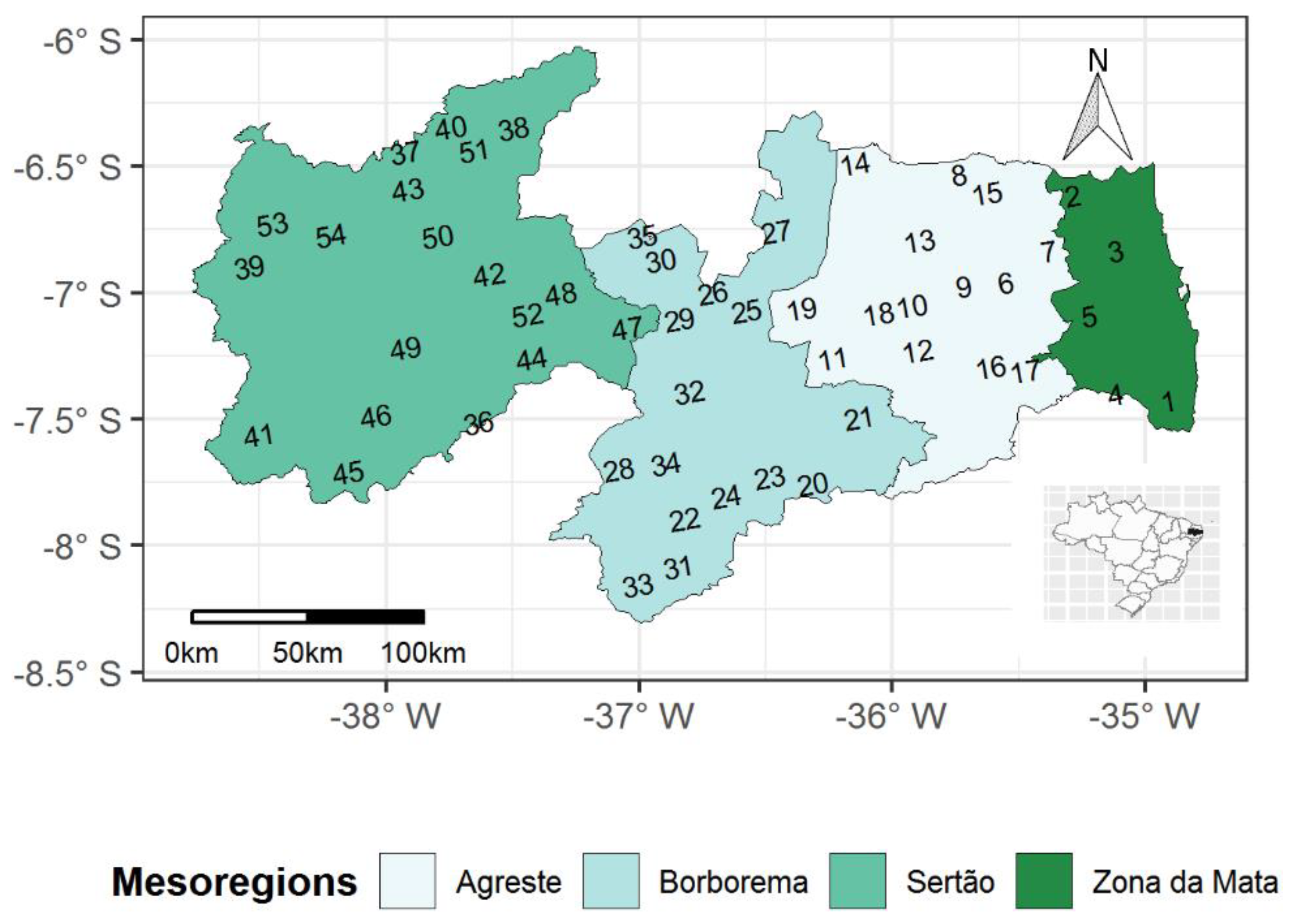
The study region was Paraíba State, Brazil (Figure 1), located in the NEB, which is positioned between parallels 6° and 8° S and meridians 34° and 39° W, with an area of approximately 56,500 km2. Paraíba is included in the Tropical Region, and its area is divided into four geographical mesoregions: Zona da Mata, Agreste, Borborema, and Sertão.
The total monthly precipitation data measured at 54 pluviometric stations were considered during the period from 1994 to 2014. Table 1 shows the identification number, name of pluviometric station, latitude, longitude, altitude above sea level, and quantiles of precipitation (mm) at 2.5%, 50%, and 97.5%.
3. Methods
In space−time geostatistics, observations are modeled as a stochastic process using a random function . We assumed that Z has the first and second moments. Thus, Z(s, t) was decomposed by the sum of the trend components and the stochastic residue:
In Equation (1), the trend component m(s, t) = E[Z(s, t)] is not constant in space and time, representing the large-scale variation. The residual component ε(s, t) describes random fluctuations on a small scale and encompasses the three components: spatial, temporal, and interaction.
3.1. Trend Component
The trend component is responsible for the large-scale variation of the stochastic process. In spatiotemporal datasets, this component is not a deterministic function. It was, therefore, necessary to specify stochastic patterns that represented the observed variability. The specification of the trend component included the geographic coordinates as covariables, as well as time. The purpose of this study was to adjust this component using GAMLSS models. In the GAMLSS models, it is assumed that the observations are independent, with and conditioned to , with So, , where G represents Z distribution. The parameters and are classified as the parameters of the location, scale, asymmetry, and kurtosis, respectively, where the latter two represent the distribution shape [14]. Thus, according to these authors, the GAMLSS models were expressed in the form,
where is a monotonic link function, and is related to explanatory variables and random effects; and are vectors of size n; is a parameter vector of size ; and are the fixed (covariate) matrices of size and , respectively; and is a random variable of dimension . In a purely parametric linear model, we have that , that is, there are no additive terms associated with the distribution parameters in the model. In the space–time case, we have .
In the modeling of the trend, the component was considered , where is the identity matrix of order and . Thus, Equation (2) is rewritten as:
The model given in Equation (3) was fitted to the data of this study, where is an unknown function of the explanatory variable and is a vector that evaluates the function in . This model is called the semiparametric additive GAMLSS and may contain parametric, nonparametric and random effects terms [14].
We considered the geographic coordinates (latitude and longitude) and the temporal index (time) as covariables to model the trend. This time index was constructed as follows: an index equal to 1 denoted Jan/1994, the index equal to 2 denoted Feb./1994, and so on. In all covariates, cubic splines (cs) were inserted, including the covariate time that was designed to model the seasonal effect of precipitation. Thus, the terms of the trend component were expressed as:
where , and represent the covariates of longitude, latitude, and time, respectively (Equation (4)). The parameters , and are related to the lease vector of the GAMLSS model, is the parameter related to the intercept for the scale vector, and is the parameter associated with covariable time and that is responsible for modeling the occurrence of no zeroes in the response variable.
In order to obtain the parameter estimates for this regression model, the penalized maximum likelihood method was used, which differs from conventional methods because it assigns the value zero to the coefficients of nonsignificant variables. However, this method does not take into account the assumption that errors are uncorrelated. Thus, it was necessary to evaluate the residuals of this model, taking into account the correlation structure. For this, we proposed to fit a valid nonseparable space–time variogram model.
3.2. Spatiotemporal Variogram
When inserting structures in the trend component, one advantage is that it describes the large-scale variation of the phenomenon being studied, causing the residuals to present small-scale variations, consequently reducing the prediction error in the kriging. After obtaining the estimates of the trend component parameters, the stochastic residue is obtained by difference, . Therefore, the next step of the analysis was the empirical estimation of the covariance function or spatiotemporal variogram to model this residue [2].
Spatiotemporal covariates are usually described using a space–time variogram , which measures the mean difference between separated data in the space–time domain using the distance vector. The estimate of this variogram, obtained by the moment’s method, was given by:
where is the cardinality for the set . It is noted in Equation (5) that the empirical variogram depends only on spatial and temporal distances, and this may not result in a valid variogram. Thus, to obtain estimates of in any arbitrary lag, the empirical variogram must be smoothed. As a solution to this limitation found in the empirical variogram, one should use a theoretical model, , which fits, as best as possible, the space–time dependence structure of the residues [15]. The vector contains all the unknown parameters to be estimated.
The typical approach is to fit a theoretical model to the empirical variogram. The least-squares estimation method is the most common approach. However, there are other methods, such as maximum likelihood, generalized estimation equations, and composite likelihood, among others [16]. In this study, the least-squares method was used.
There are no assumptions about the probability distribution of the empirical variogram’s generated values in the least-squares method. The approach considers the statistical model of the form . Assume that has null mean and covariance matrix , which depends on . We suggested that the diagonal of can be approximated to:
where is the number of pairs at each space–time distance. Thus, the weights assigned in the weighting matrix are proportional to the number of pairs in a given space–time distance.
The adjustment of the theoretical space–time variogram model was made by using the weighted least-squares (WLS) method, which replaces with the diagonal matrix . The elements of were obtained from Equation (6). Thus, using the weights given in this Equation (7), the WLS method is given by:
Generally, statistical assumptions are considered, which comprise a space–time covariance function and ensure that this function is defined as positive [17,18,19]. Several researchers have studied the construction of valid space–time covariance functions [15,20,21]. Although this type of construction is a difficult task, the complexity becomes more significant when it is desired to determine valid models of space–time covariance. In the space–time approach, there are two types of general model classes: the separable and the nonseparable.
The separable models assume that spatial and temporal processes are uncorrelated and that variograms are composed of purely spatial and purely temporal models. As an example, the space–time covariance function can be expressed as the product between purely spatial and purely temporal components. The major drawback of this type of model is the nonincorporation of the spatial–temporal interaction component [18]. However, the nonseparable models assume that the space–time phenomenon is correlated in space–time [22]. We used the generalized sum–product model, which belongs to the nonseparable covariance model class.
The stationary covariance model product–sum [17,23] is given by . Assuming that is second-order stationary, we have that: and in which, based on the assumption of second-order stationarity, we have that the product–sum covariance function is defined as:
where , e are constants that ensure that the covariance function is positive definite (Equation (8)). e are the spatial and temporal thresholds, respectively. Applying the relation, , we have the product–sum variogram. This model gives origin to the following relations:
where and are the proportionality coefficients between the space–time variograms, and , and the spatial and temporal variograms, and , respectively. Therefore, modeling is equivalent to modeling . Likewise, estimating and modeling is equal to estimating and modeling . The two relations established in Equation (9) can be simplified by imposing three constraints: and
These constraints facilitate the estimation of the model parameters and using and , for this it is necessary to determine , , and . These three coefficients of the model can be written in terms of the thresholds and parameters and [17]. In this particular case, this leads to modeling and , using the models of and , respectively. In addition, these two parameters were combined into a single parameter k, resulting in the generalized product–sum model (Equation (10)).
By combining the parameters and to form a single parameter k, the space–time variogram expression, , was simplified to,
where . In Equation (11), the parameter k is expressed as:
We used the covariance generalized product–sum model, and the variogram function of this model is expressed by:
where and are the marginal spatial and temporal variograms, respectively (Equation (12)). The great advantage of this type of model is that sample-based marginal adjustments are used, and only one global threshold parameter is incorporated for space–time interaction [24]. In Equation (13) the parameter k is positive and has an identity involving the global threshold, together with the spatial and temporal threshold, and , respectively, given by:
3.3. Geostatistical Prediction
Once the trend component was determined and estimated and a valid space–time variogram model fitted, the next step consisted of the space–time kriging of the residuals using the ordinary kriging method. The variogram model is crucial in space–time kriging to calculate the best invariant linear predictor. Thus, it was necessary to obtain the space–time kriging equations, which provide the weights of the observations in such a predictor and the prediction variation that indicates the prediction accuracy [1].
Ordinary space–time kriging [15] consists of predicting the value at the nonsampled space–time point , from the stochastic component . For this, the linear predictor, is used, where are the kriging weights obtained by imposing the condition that the prediction error expectation is zero and that it has minimum variance; that is, it is the best linear unbiased predictor (BLUP). To obtain the weights, we used the ordinary space–time kriging equations that were calculated in terms of the variogram:
In the system of Equations (14), α is the Lagrange multiplier required to minimize the prediction variance. The prediction variance (Equation (15)) is given by:
in which the final predictor () for the precipitation variable (), at the location , is defined as:
where is the estimated value for the location obtained by adjusting GAMLSS models (Equation (16)). Figure 2 shows the flowchart of regression kriging with GAMLSS model.
The interpolation performance in space–time kriging was evaluated using the leave-one-out method, which consisted of removing an observed point from the precipitation in space–time and then predicting its value . This process was then repeated for all remaining points, and the residue (E) of this procedure was then obtained by the difference between the observed and predicted values at each location . After that, the RMSE (root mean squared error), MAE (mean absolute error), and R2 (coefficient of determination) were extracted as selection criteria.
4. Results
4.1. Descriptive Analysis
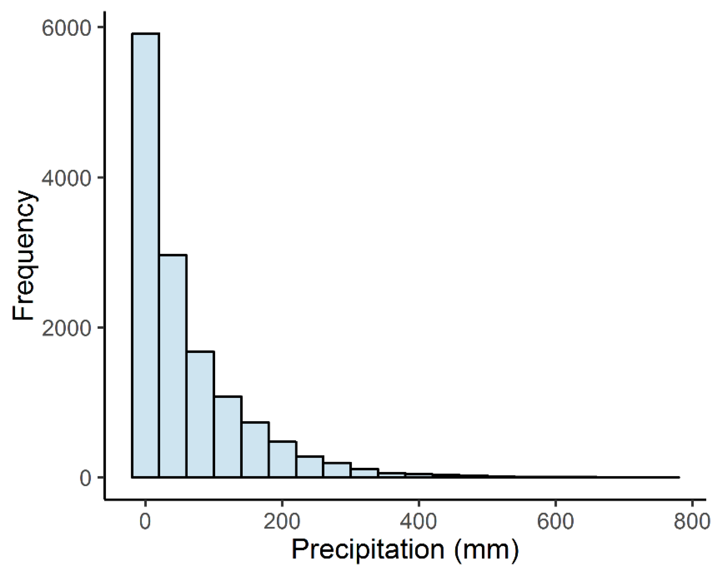
The precipitation variable, measured monthly in each of the 54 locations, in the period 1994–2014, presented a median value of 29.05 mm and an interquartile range of 3.60–90.20 mm. In the whole historical series, approximately 20% of the observations presented 0.00 mm of total monthly precipitation. In order to evaluate the precipitation distribution of the studied region, a histogram was initially developed for the entire dataset (Figure 3).
In Figure 3, it is possible to observe the excess of zeroes values in the dataset and, consequently, the presence of asymmetric behavior, indicating that the Gaussian model is not the most suitable for modeling.
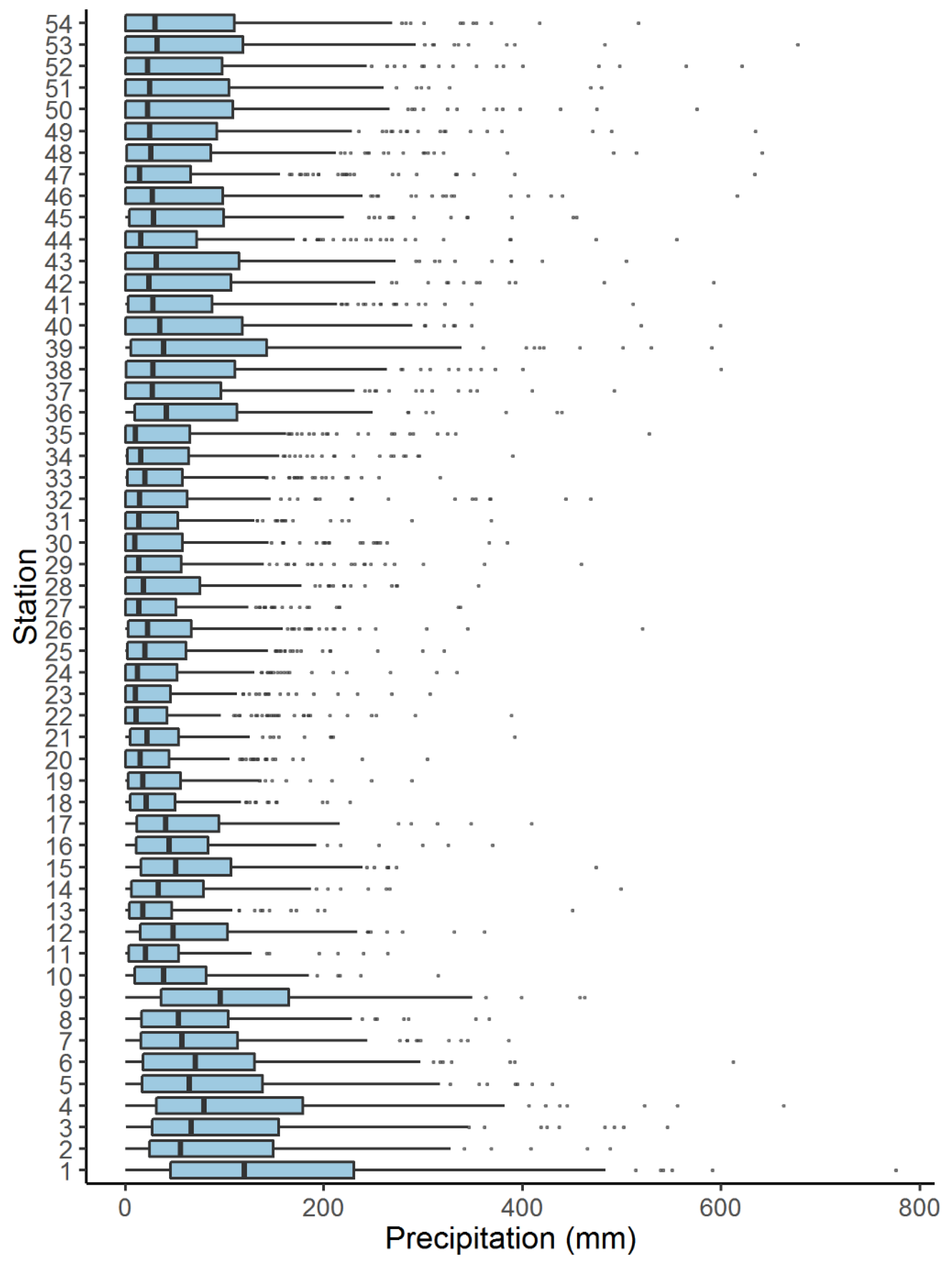
Box plots were built to explore the behavior of precipitation at the 54 pluviometric stations (Figure 4).
Due to the asymmetric behavior and the high variability of precipitation, the State of Paraíba suffers from irregular distribution of rainfall throughout the region. This distribution presented high variability among the mesoregions analyzed in this work. A positive asymmetry was observed in all the locations, as well as the presence of atypical points (Figure 4).
4.2. Trend Analysis
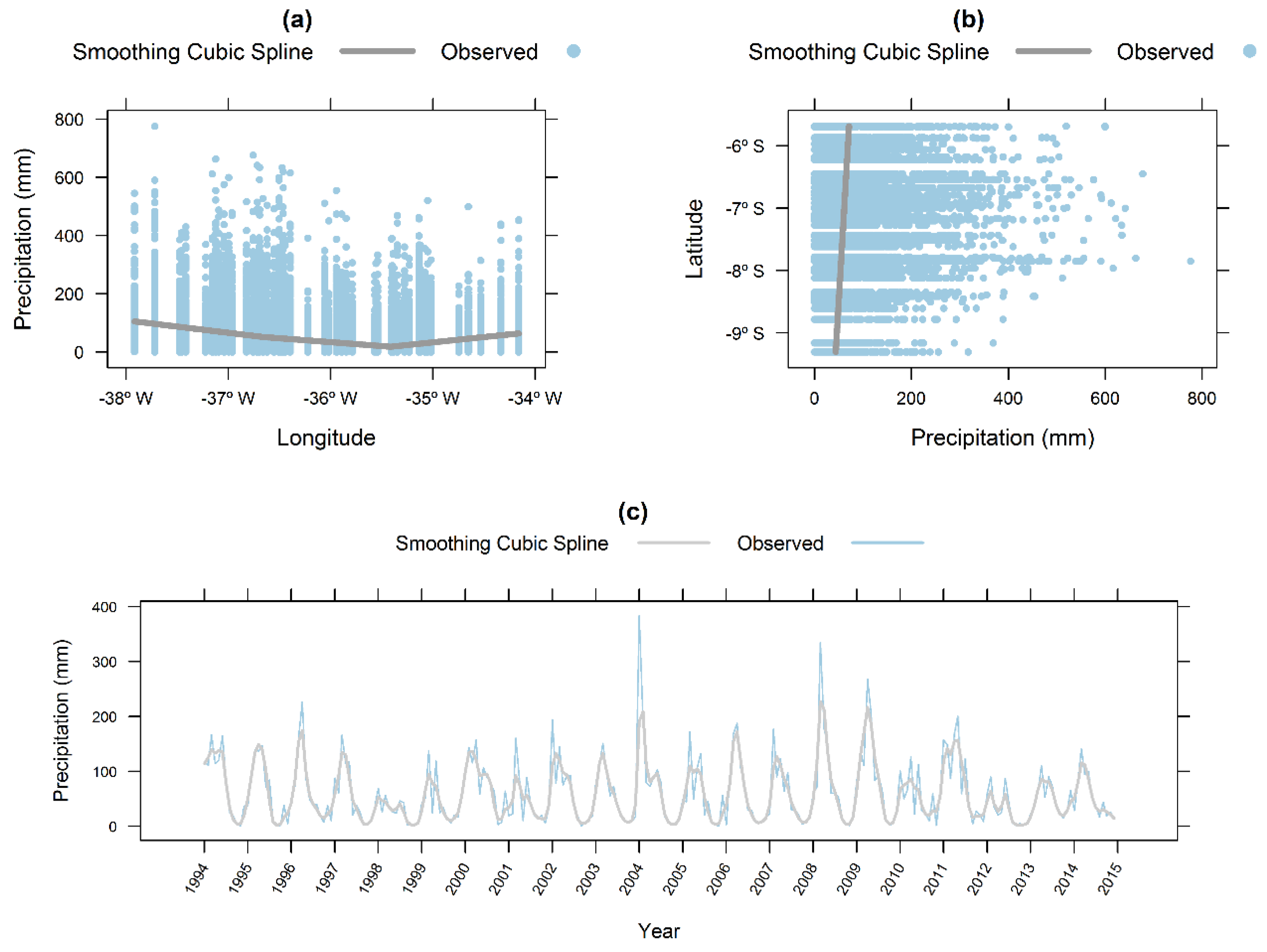
The distribution of precipitation relative to geographical coordinates (latitude and longitude) and temporal index, with the corresponding adjustments through cubic splines, is presented in Figure 5.
An exploratory analysis by adjusting the cubic smoothness function of the spline showed that precipitation occurred more frequently in the extremes of the studied region, corresponding to the mesoregions of Sertão and Zona da Mata, and that there was limited precipitation in the areas located near the meridian 36° W, corresponding to the Borborema mesoregion (Figure 5a). The spatial distribution of rainfall in the region presented a spatial tendency that varied with the latitudinal and longitudinal gradients (Figure 5a,b). For the analysis of the time trend, the graph of the time series of precipitation was calculated, based on the average of 54 pluviometric stations (Figure 5c). This series showed an evident seasonal behavior of 12 months. Thus, for this series, a GAMLSS model was fitted using cubic smoothing splines function.
To model the trend of precipitation data, the GAMLSS model was used, via zero-adjusted gamma (ZAGA) distribution, as indicated in the system of Equations (4). Table 2 presents the coefficient estimates, standard error, t value, p-value, and the coefficient of determination (R2) in the model adjustment.
The results presented in Table 2 indicate, at the level of 0.01 of significance, that the covariates longitude, latitude, and the temporal index are related to the precipitation. The R2 shows that 48% of the large-scale variation of rainfall was explained by the trend component, corroborating with the results found through the descriptive analysis.
After estimating the trend component, which was described in Equation (1), we then analyzed the stochastic residue, . Next, the space–time sampling variogram of these residues was calculated, taking as reference the adjustment of the generalized product–sum theoretical model.
4.3. Geostatistical Analysis
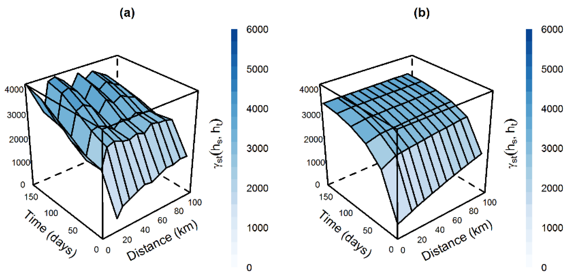
The residuals, obtained from the regression via GAMLSS models, presented an evident pattern of spatiotemporal correlation (Figure 6a). There was a strong spatial correlation between nearby sites, and the spatial structure became weaker as time differences increased. Similarly, the same occurred with the temporal structure (Figure 6b). Thus, spatial–temporal kriging of the residue was required.
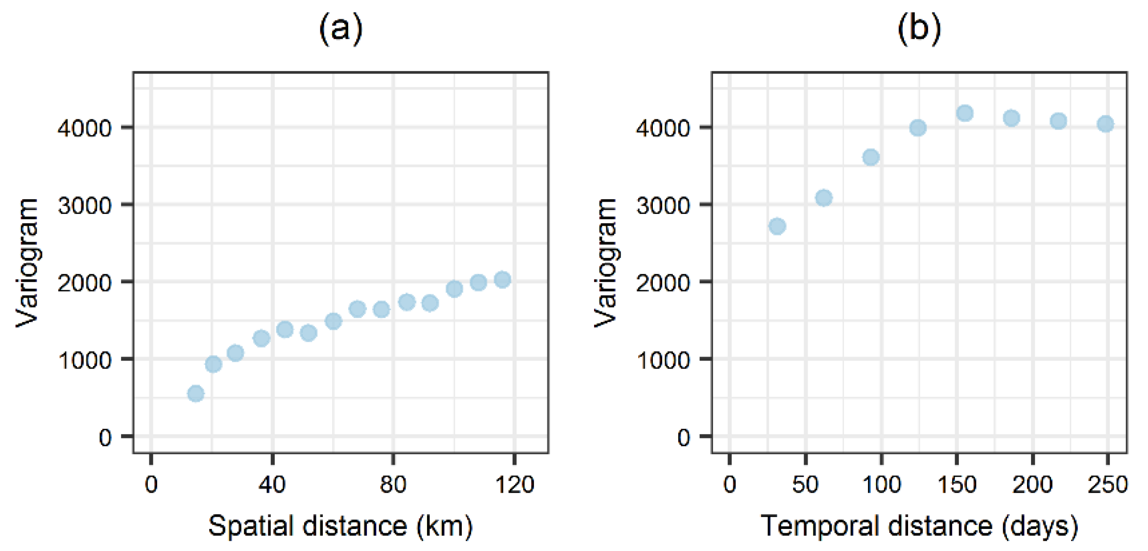
The behavior of the empirical space–time variogram estimates is presented in terms of the marginal effects (Figure 7).
The spatial variability exhibited by the marginal spatial variogram (Figure 7a) differed from the temporal variability shown in the marginal temporal variogram (Figure 7b), since a difference, concerning the threshold, was observed between the two marginal variograms. For this reason, the spatiotemporal variability of the residues could be modeled through the generalized product–sum model. One of the advantages of constructing marginal variograms is the fact that it is possible to identify some theoretical variogram models (for example, Gaussian, Exponential, and Spherical) that can compose the structure in the generalized product–sum model (Equation (12)).
As described above, the Normal, Gamma, and ZAGA models have been adjusted for large-scale variations. The different structures of the generalized product–sum model were adjusted for the residues obtained in each of these models, followed by the spatial–temporal kriging of that model. The cross-validation results are provided in Table 3. The results of the validation were calculated after the values adjusted by the trend component were added to the values interpolated in space–time kriging.
The results presented in Table 3 indicate that the Exponential model was the best fit for the spatial () and temporal () structures in all regression models, since it presented higher R2 and smaller RMSE and MAE. Note that the ZAGA model (EXP + EXP) presented the best results, with RMSE of 34.598 mm, MAE of 20.970 mm, and R2 equal to 82.8%. These results demonstrated the effectiveness of adjusting the precipitation data to an adequate model that contemplates the spatial–temporal characteristics presented by the phenomenon.
The components of the generalized product–sum model (Equation (12)) and their estimates are shown in Table 4. The components were chosen based on the results in Table 3.
The parameter estimates (Table 4) indicated that all components act on the spatial–temporal pattern of the ZAGA regression residuals. The parameter estimation related to the spatial extent was high, indicating that the residues were correlated in distances of up to 171 km. The temporal scale estimate indicated that sites with a delay of up to 47 days had residual autocorrelation.
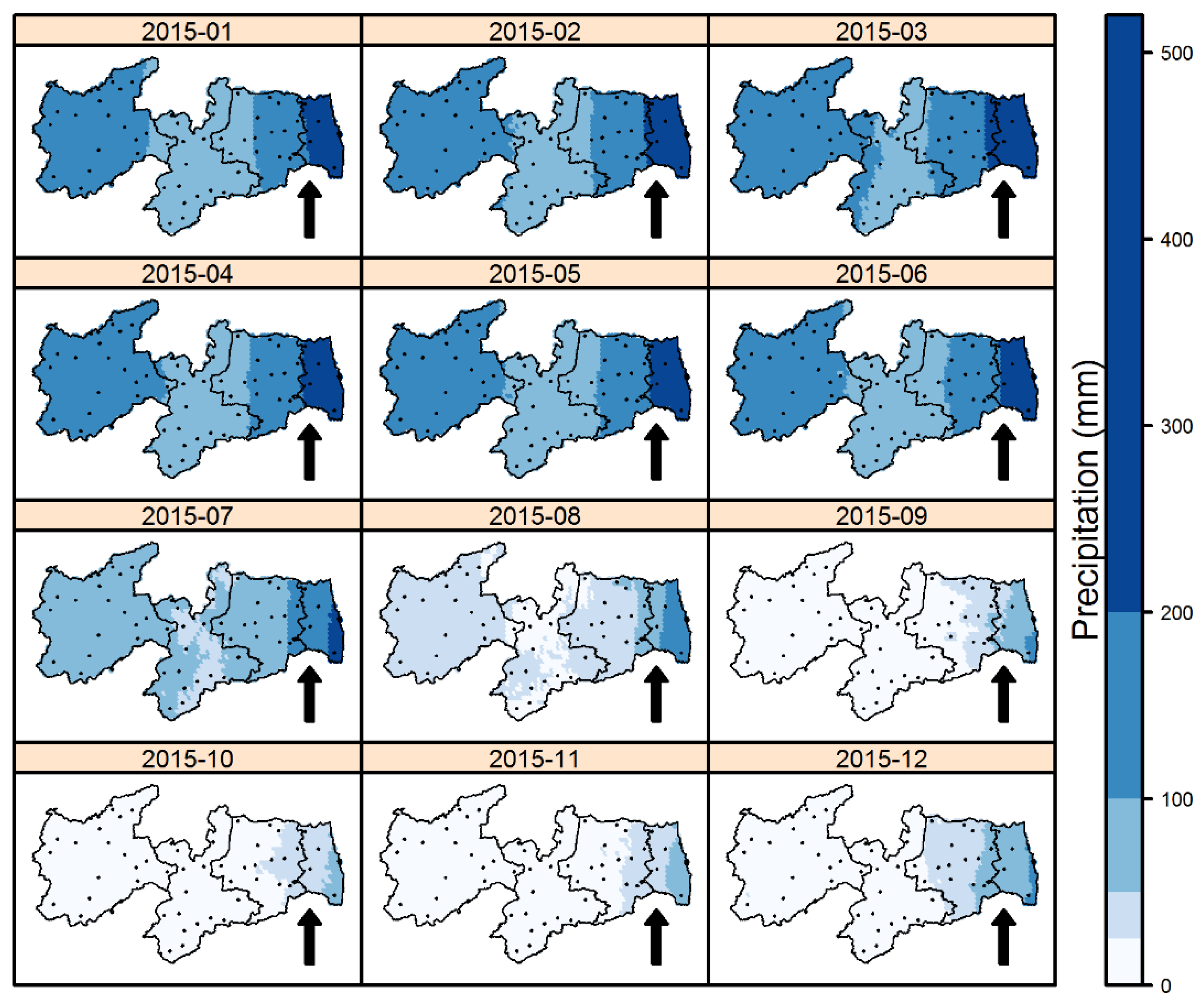
The main advantage of the methodology proposed in this study is that with the space–time kriging technique, predictions can be made for unobserved locations and times [21,24]. As an example of this methodology applicability, the spatial–temporal kriging of precipitation was carried out in the period 2015 (Figure 8).
In Figure 8, it is possible to evaluate the precipitation behavior in nonsampled sites, as well as in times not observed in the sample, helping policymakers manage the allocation of water in the present and the future. It is noted that the spatial distribution of rainfall presented variability within each mesoregion and also among the four mesoregions. Precipitation in the region occurred more intensely during the first half of the year, but during the same period, there was an irregularity in the distribution of rainfall between the mesoregions. In the Sertão, the high spatial variability can be justified by meteorological systems in the area, such as the the Intertropical Convergence Zone (ITCZ) and the Upper Tropospheric Cyclonic Vortices (UTCV). It is observed that in this region, the rainfall distribution during February to May occurred irregularly. In years when El Niño and La Niña occurred with strong intensity, there was substantial evidence that rainfall occurred, respectively, above or below the expected value, resulting in high temporal variability of precipitation [27]. The rainy season in this area is concentrated between February and May, presenting high variation in space and time. The low volume of rainfall and the irregularity of its distribution have contributed, for example, to the occurrence of the desertification phenomenon [5,28].
5. Discussion
The state of Paraíba has abnormalities in the distribution of precipitation, with high spatial and temporal variability, resulting in heavy rains with short duration and prolonged periods of drought. Consequently, the scarcity of rain directly affects water resources, resulting in severe problems in the region’s economy, which focuses on family agriculture and livestock [29]. Also, drought has affected water distribution for human consumption, electricity supply, the occurrence of diseases and migration, among other issues, resulting in an unprecedented water crisis [30]. Thus, a space–time distribution modeling of rainfall becomes of paramount importance for the water resources management to reduce the impacts caused by drought in this region.
Irregular rainfall, resulting in periods of prolonged drought, is associated with meteorological phenomena. Strong El Niño years have caused intense droughts in Paraíba [27]. Rainfall periods are concentrated in a few months, occurring mainly in winter, which is associated with the ITCZ action and the passage of cold fronts from the South Atlantic Ocean [31]. Due to the high rainfall variability of the region, rainfall behavior can be classified into three periods, namely: pre-rainy season, rainy season and post-rainy season. During the pre-rainy season, which runs from December to January in the Sertão mesoregion, meteorological systems such as UTCV and instability associated with cold fronts occur. The rainy season itself persists from February to May, when the ITCZ acts as the primary meteorological system responsible for the recharge of water resources in the state. The post-rainy season usually occurs between May and July in the Zona da Mata mesoregion and some localities of the Southeast. The Eastern Wave Disturbances (EWDs) are the primary meteorological system acting in this period.
In this study, we used the gamma distribution, which shows asymmetric behavior, to model precipitation data. However, it is known that this probability distribution does not include values equal to zero, not having a parameter that can be used to model the excess of zero that is common in data of monthly total precipitation throughout the NEB. As an advantage, the methodology allowed modeling the occurrence of null values, resulting in better estimates when compared with models that do not contemplate the excess of zeroes in the dataset.
Several studies that deal with spatial–temporal modeling and which have null values in the database have used the regression model with Normal distribution [11,32] or the Gamma regression model [12,13]. However, the Normal regression does not solve the data asymmetry problem, and the Gama regression does not contemplate in its domain the occurrence of zeroes. Thus, we propose a new way of modeling the trend component through GAMLSS models, especially using the ZAGA distribution, allowing one of its three parameters to model the excess of zeroes that occurs with high frequency in data of monthly total precipitation.
The trend component alone does not model the spatiotemporal dependence that is present in the regression residuals. Thus, the need for space–time modeling of these residues arises. Previous studies did not take into account this spatial and/or temporal residue dependence [7,33]. Consequently, we modeled the spatiotemporal dependence structure of this stochastic component, using a covariance function. However, this approach has numerous parameters present in the space–time theoretical variogram, resulting in great computational difficulties to determine the parameter estimates.
A significant benefit of the suggested methodology is that it can predict in nonsampled places and in periods that have not been observed, thereby assisting water-related initiatives in the region. The Agreste and Borborema mesoregions, with a reduced amount of precipitation, were discovered to be an aggravating factor in the uneven rainfall distribution in the study region. The majority of the state of Paraíba is part of the Brazilian semi-arid region, which has a climate characterized by low humidity and rainfall. Studies in recent years have revealed the process of desertification in the semi-arid Northeast regions [30]. This research can, therefore, identify areas that will soon be affected by water supplies for human and animal consumption. These findings can serve as a supporting tool to help government agencies in water management to predict societal needs and avoid water shortages that are rapidly intensifying, not only in Paraíba State, but also in the NEB as a whole.
6. Conclusions
In this study, total monthly precipitation in the state of Paraíba was analyzed using spatiotemporal geostatistical tools. Rainfall data of 54 pluviometric stations from 1994 to 2014 were analyzed. Large-scale variation was modeled using spatial and temporal covariates to remove the spatiotemporal trend in the regression residuals. It was proposed to use the adjustment of GAMLSS models with different distributions for the response variable (Normal, Gamma, and ZAGA). The results of the cross-validation indicated that the ZAGA distribution best fits the data, with the exponential model for the spatial component and also for the time component of the generalized product–sum variogram model. Also, the results indicated the presence of the space–time correlation in the rainfall phenomenon, implying in this way the proper use of space–time kriging proposed in this study. Finally, space–time kriging in Paraíba state for the year 2015 evidenced the great irregularity in the distribution of rainfall throughout the region, providing a detailed visual analysis of sectors suffering from scarcity and excess of rain, favoring government policies that address water resources.
Author Contributions
Conceptualization, E.S.d.M., R.R.d.L., R.A.d.O., L.G.D. and C.A.C.d.S.; Methodology, E.S.d.M., R.R.d.L. and R.A.d.O; Software, E.S.d.M.; Validation, E.S.d.M. and R.R.d.L.; Formal analysis, E.S.d.M., R.R.d.L., R.A.d.O., L.G.D. and C.A.C.d.S.; Investigation, E.S.d.M., R.R.d.L., R.A.d.O., L.G.D. and C.A.C.d.S.; Resources, E.S.d.M.; Data curation, E.S.d.M. and C.A.C.d.S.; Writing—original draft preparation, E.S.d.M., R.R.d.L., R.A.d.O., L.G.D. and C.A.C.d.S.; Writing—review and editing, E.S.d.M., R.R.d.L., R.A.d.O., L.G.D. and C.A.C.d.S.; Visualization, E.S.d.M.; supervision, E.S.d.M., R.R.d.L., R.A.d.O. and C.A.C.d.S.
Funding
This research was funded by the Brazilian National Council for Scientific and Technological Development (CNPq) and the Brazilian Federal Agency for the Support and Evaluation of Graduate Education (CAPES).
Acknowledgments
The authors acknowledge the Brazilian National Council for Scientific and Technological Development (CNPq) and the Coordination for the Improvement of Higher Education Personnel (CAPES)-Finance Code 001 (Pró-Alertas Research Project-Grant No. 88887.091737/2014-01 and 88887.123949/2015-00). We thank Lacey Bodnar from the Robert B. Daugherty Water for Food Global Institute (DWFI) at the University of Nebraska for her invaluable assistance, and the support of DWFI is also appreciated.
Conflicts of Interest
The authors declare no conflict of interest.
References
- Kilibarda, M.; Tadić, M.P.; Hengl, T.; Luković, J.; Bajat, B. Global geographic and feature space coverage of temperature data in the context of spatio-temporal interpolation. Spat. Stat. 2015, 14, 22–38. [Google Scholar] [CrossRef]
- Martínez, W.A.; Melo, C.E.; Melo, O.O. Median Polish Kriging for space-time analysis of precipitation. Spat. Stat. 2017, 19, 1–20. [Google Scholar] [CrossRef]
- Stauffer, R.; Mayr, G.J.; Messner, J.W.; Umlauf, N.; Zeileis, A. Spatio-temporal precipitation climatology over complex terrain using a censored additive regression model. Int. J. Climatol. 2017, 37, 3264–3275. [Google Scholar] [CrossRef] [PubMed]
- Marengo, J.A.; Torres, R.R.; Alves, L.M. Drought in Northeast Brazil—past, present, and future. Theor. Appl. Climatol. 2017, 129, 1189–1200. [Google Scholar] [CrossRef]
- Borges, B.C.; de Baptista, G.M.; Meneses, P.R. Identification of hydromorphic areas by means of spectral analysis of remote sensing data, as support for the preparation of forensic reports issued to evaluation of rural properties. Rev. Bras. Geogr. Física 2014, 7, 1062–1077. [Google Scholar] [CrossRef]
- De Almeida, H.A.; Medeiros, E.A. Variabilidade no regime pluvial em duas mesorregiõres da Paraíba e sua relação com o fenômeno EL Niño Oscilação Sul. J. Environ. Anal. Prog. 2017, 2, 177. [Google Scholar] [CrossRef]
- Dos Santos, C.A.C.; Gomes, O.M.; de Souza, F.A.S.; Paiva, W. De Análise Geoestatística da Precipitação Pluvial do Estado da Paraíba (Geostatistical Analysis of Precipitation in Paraiba State). Rev. Bras. Geogr. Física 2012, 4, 692. [Google Scholar] [CrossRef]
- Francisco, P.R.M.; da Mello, V.S.; Bandeira, M.M.; de Marcedo, F.L.; Santos, D. Discriminação de cenários pluviométricos do estado da Paraíba utilizando distribuição Gama Incompleta e Teste Kolmogorov-Smirnov. Rev. Bras. Geogr. Física 2016, 9, 41–61. [Google Scholar]
- Gräler, B.; Gerharz, L.; Pebesma, E. Spatio-temporal analysis and interpolation of PM10 measurements in Europe. ETC/ACM Tech. Pap. 2011/10 2012, 8, 37. [Google Scholar]
- Hengl, T.; Heuvelink, G.B.M.; Perčec Tadić, M.; Pebesma, E.J. Spatio-temporal prediction of daily temperatures using time-series of MODIS LST images. Theor. Appl. Climatol. 2012, 107, 265–277. [Google Scholar] [CrossRef]
- Hu, D.; Shu, H.; Hu, H.; Xu, J. Spatiotemporal regression Kriging to predict precipitation using time-series MODIS data. Cluster Comput. 2017, 20, 347–357. [Google Scholar] [CrossRef]
- Menezes, R.; Piairo, H.; García-Soidán, P.; Sousa, I. Spatial–temporal modellization of the NO2 concentration data through geostatistical tools. Stat. Methods Appt. 2016, 25, 107–124. [Google Scholar] [CrossRef]
- Monteiro, A.; Menezes, R.; Silva, M.E. Modelling spatio-temporal data with multiple seasonalities: The NO2 Portuguese case. Spat. Stat. 2017, 22, 371–387. [Google Scholar] [CrossRef]
- Stasinopoulos, M.; Rigby, R.A.; Heller, G.Z.; Voudouris, V.; De Bastiani, F. Flexible Regression and Smoothing Using GAMLSS in R; CRC Press: New York, NY, USA, 2017. [Google Scholar]
- Montero, J.-M.; Fernández-Avilés, G.; Mateu, J. Spatial and Spatio-Temporal Geostatistical Modeling and Kriging; John Wiley & Sons, Ltd: Chichester, UK, 2015. [Google Scholar]
- Schabenberger, O.; Gotway, C.A. Statistical Methods for Spatial Data Analysis; CRC Press: New York, NY, USA, 2004. [Google Scholar]
- Iaco, S.D.; Myers, D.E.; Posa, D. Space–time analysis using a general product–sum model. Stat. Probab. Lett. 2001, 52, 21–28. [Google Scholar] [CrossRef]
- Huang, H.-C.; Martinez, F.; Mateu, J.; Montes, F. Model comparison and selection for stationary space–time models. Comput. Stat. Data Anal. 2007, 51, 4577–4596. [Google Scholar] [CrossRef]
- Cressie, N.; Wikle, C.K. Statistics for Spatio-Temporal Data; John Wiley & Sons, Inc.: Hoboken, NJ, USA, 2015. [Google Scholar]
- Iaco, S.D.; Myers, D.E.; Posa, D. Nonseparable space-time covariance models: Some parametric families. Math. Geol. 2002, 34, 23–42. [Google Scholar] [CrossRef]
- Kilibarda, M.; Hengl, T.; Heuvelink, G.B.M.; Gräler, B.; Pebesma, E.; Perčec Tadić, M.; Bajat, B. Spatio-temporal interpolation of daily temperatures for global land areas at 1 km resolution. J. Geophys. Res. Atmos. 2014, 119, 2294–2313. [Google Scholar] [CrossRef]
- Sherman, M. Spatial Statistics and Spatio-Temporal Data; Wiley Series in Probability and Statistics; John Wiley & Sons, Ltd.: Chichester, UK, 2010. [Google Scholar]
- Cesare, L.D.; Myers, D.; Posa, D. Estimating and modeling space–time correlation structures. Stat. Probab. Lett. 2001, 51, 9–14. [Google Scholar] [CrossRef]
- Iaco, S.D.; Palma, M.; Posa, D. Spatio-temporal geostatistical modeling for French fertility predictions. Spat. Stat. 2015, 14, 546–562. [Google Scholar] [CrossRef]
- Graler, B.; Pebesma, E.; Heuvelink, G. Spatio-temporal interpolation using gstat. Wp 2016, 8, 1–20. [Google Scholar] [CrossRef]
- Bivand, R.S.; Pebesma, E.; Gómez-Rubio, V. Hello World: Introducing Spatial Data. In Applied Spatial Data Analysis with R; Springer: New York, NY, USA, 2013; pp. 1–16. [Google Scholar]
- Marengo, J.A.; Alves, L.M.; Alvala, R.C.; Cunha, A.P.; Brito, S.; Moraes, O.L.L. Climatic Characteristics of the 2010–2016 Drought in the Semiarid Northeast Brazil Region. 2017. Available online: http://www.scielo.br/scielo.php?script=sci_arttext&pid=S0001-37652018000501973 (accessed on 7 November 2019).
- Souza, B.I.; Menezes, R.; Artigas, R.C. Efeitos da desertificação na composição de espécies do bioma Caatinga, Paraíba/Brasil. Investig. Geográficas 2015, 45–59. [Google Scholar] [CrossRef]
- Macedo, M.J.; Guedes, R.; de Sousa, F.A.; Dantas, F. Analysis of the standardized precipitation index for the Paraíba state, Brazil. Ambient. e Agua-An Interdiscip. J. Appl. Sci. 2010, 5, 204–214. [Google Scholar] [CrossRef]
- Gutiérrez, A.P.A.; Engle, N.L.; De Nys, E.; Molejón, C.; Martins, E.S. Drought preparedness in Brazil. Weather Clim. Extrem. 2014, 3, 95–106. [Google Scholar] [CrossRef] [Green Version]
- Rodrigues, R.R.; McPhaden, M.J. Why did the 2011–2012 La Niña cause a severe drought in the Brazilian Northeast? Geophys. Res. Lett. 2014, 41, 1012–1018. [Google Scholar] [CrossRef]
- Guo, L.; Lei, L.; Zeng, Z.-C.; Zou, P.; Liu, D.; Zhang, B. Evaluation of spatio-temporal variogram models for mapping Xco2 using satellite observations: A case study in China. IEEE J. Sel. Top. Appl. Earth Obs. Remote Sens. 2015, 8, 376–385. [Google Scholar] [CrossRef]
- Gomes, O.M.; dos Santos, C.A.C.; de Souza, F.A.S.; de Paiva, W.; de Olinda, R.A. Análise comparativa da precipitação no estado da paraíba utilizando modelos de regressão polinomial. Rev. Bras. Meteorol. 2015, 30, 47–58. [Google Scholar] [CrossRef]
Figure 1.
Pluviometric stations over the four mesoregions of Paraíba State, Brazil. The information for each respective number is presented in Table 1.
Figure 1.
Pluviometric stations over the four mesoregions of Paraíba State, Brazil. The information for each respective number is presented in Table 1.

Figure 2.
Regression kriging flowchart with GAMLSS model. GAMLSS: generalized additive models for location, scale, and shape.
Figure 2.
Regression kriging flowchart with GAMLSS model. GAMLSS: generalized additive models for location, scale, and shape.

Figure 3.
Histogram of the precipitation data of the 54 pluviometric stations sampled in the period from 1994 to 2014.
Figure 3.
Histogram of the precipitation data of the 54 pluviometric stations sampled in the period from 1994 to 2014.

Figure 4.
Box plot of monthly rainfall for 54 pluviometric stations, listed in Table 1, in this study.
Figure 4.
Box plot of monthly rainfall for 54 pluviometric stations, listed in Table 1, in this study.

Figure 5.
Distribution of precipitation data (mm) (blue dots) in the longitude direction (a) and in the latitude direction (b) and respective trend lines (gray line) using cubic smoothing splines function over the study region; time series of precipitation data (mm) (blue line) and adjusted temporal trend (gray line) (c).

Figure 6.
Empirical space–time variogram (a) and adjusted variogram (b).

Figure 7.
Marginal experimental variograms of the residuals: purely spatial (a) and purely temporal (b).
Figure 7.
Marginal experimental variograms of the residuals: purely spatial (a) and purely temporal (b).

Figure 8.
Spatial–temporal prediction of total monthly rainfall (mm) in the study region for the year 2015. The crosses (+) represent the positions of each pluviometric station.
Figure 8.
Spatial–temporal prediction of total monthly rainfall (mm) in the study region for the year 2015. The crosses (+) represent the positions of each pluviometric station.


Table 1.
Pluviometric stations with an identification number (ID), name of the mesoregion, name of rainfall station, latitude (Lat), longitude (Long), Altitude (Alt), and precipitation quantiles 2.5%, 50%, 97.5%.
Table 1.
Pluviometric stations with an identification number (ID), name of the mesoregion, name of rainfall station, latitude (Lat), longitude (Long), Altitude (Alt), and precipitation quantiles 2.5%, 50%, 97.5%.
| ID | Mesoregion | Station | Lat | Long | Alt (m) | Quantiles | ||
|---|---|---|---|---|---|---|---|---|
| 2.5% | 50.0% | 97.5% | ||||||
| 1 | Zona da Mata | Alhandra | −7.43 | −34.91 | 56.28 | 6.49 | 119.85 | 481.71 |
| 2 | Zona da Mata | Jacaraú | −6.61 | −35.29 | 181.19 | 0.88 | 55.90 | 311.01 |
| 3 | Zona da Mata | Mamanguape | −6.84 | −35.12 | 16.62 | 2.60 | 66.70 | 403.02 |
| 4 | Zona da Mata | Pedras de Fogo | −7.40 | −35.12 | 175.36 | 4.71 | 79.25 | 399.52 |
| 5 | Zona da Mata | Sapé | −7.09 | −35.22 | 116.84 | 1.86 | 64.35 | 324.14 |
| 6 | Agreste | Alagoinha | −6.96 | −35.55 | 168.64 | 0.00 | 70.50 | 306.56 |
| 7 | Agreste | Araçagi | −6.83 | −35.39 | 104.62 | 0.00 | 56.95 | 290.73 |
| 8 | Agreste | Araruna | −6.53 | −35.74 | 575.41 | 0.00 | 53.40 | 235.32 |
| 9 | Agreste | Areia | −6.98 | −35.72 | 572.28 | 4.34 | 95.55 | 331.73 |
| 10 | Agreste | Areial | −7.05 | −35.93 | 693.09 | 0.00 | 38.55 | 182.72 |
| 11 | Agreste | Boa Vista | −7.26 | −36.24 | 486.00 | 0.00 | 20.30 | 127.07 |
| 12 | Agreste | Campina Grande | −7.23 | −35.90 | 544.37 | 0.93 | 48.00 | 244.28 |
| 13 | Agreste | Casserengue | −6.79 | −35.89 | 396.63 | 0.00 | 18.00 | 137.88 |
| 14 | Agreste | Cuité | −6.49 | −36.15 | 668.96 | 0.00 | 33.35 | 190.79 |
| 15 | Agreste | Dona Inês | −6.61 | −35.63 | 421.72 | 0.00 | 51.25 | 242.04 |
| 16 | Agreste | Ingá | −7.29 | −35.61 | 155.56 | 0.00 | 44.35 | 191.81 |
| 17 | Agreste | Mogeiro | −7.31 | −35.48 | 108.28 | 0.00 | 40.95 | 194.68 |
| 18 | Agreste | Pocinhos | −7.08 | −36.06 | 650.32 | 0.00 | 21.45 | 140.05 |
| 19 | Agreste | Soledade | −7.06 | −36.36 | 523.63 | 0.00 | 17.75 | 139.61 |
| 20 | Borborema | Barra de São Miguel | −7.75 | −36.32 | 488.63 | 0.00 | 15.30 | 142.21 |
| 21 | Borborema | Boqueirão | −7.49 | −36.14 | 355.08 | 0.00 | 21.65 | 148.11 |
| 22 | Borborema | Camalaú | −7.89 | −36.83 | 519.16 | 0.00 | 11.15 | 185.53 |
| 23 | Borborema | Caraúbas | −7.73 | −36.49 | 442.24 | 0.00 | 10.60 | 161.65 |
| 24 | Borborema | Congo | −7.80 | −36.66 | 491.99 | 0.00 | 12.25 | 164.82 |
| 25 | Borborema | Juazeirinho | −7.07 | −36.58 | 553.96 | 0.00 | 20.10 | 175.97 |
| 26 | Borborema | Junco do Seridó | −7.00 | −36.71 | 589.56 | 0.00 | 22.40 | 210.18 |
| 27 | Borborema | Pedra Lavrada | −6.76 | −36.46 | 521.82 | 0.00 | 13.55 | 180.72 |
| 28 | Borborema | Prata | −7.70 | −37.08 | 584.00 | 0.00 | 18.85 | 220.19 |
| 29 | Borborema | Salgadinho | −7.10 | −36.85 | 430.45 | 0.00 | 13.60 | 240.85 |
| 30 | Borborema | Santa Luzia | −6.87 | −36.92 | 311.24 | 0.00 | 9.80 | 246.99 |
| 31 | Borborema | São João do Tigre | −8.08 | −36.85 | 572.84 | 0.00 | 13.80 | 161.03 |
| 32 | Borborema | São José dos Cordeiros | −7.39 | −36.81 | 530.49 | 0.00 | 14.30 | 313.51 |
| 33 | Borborema | São Seb. do Umbuzeiro | −8.15 | −37.01 | 595.79 | 0.00 | 20.10 | 200.60 |
| 34 | Borborema | Sumé | −7.67 | −36.90 | 519.88 | 0.00 | 15.70 | 264.53 |
| 35 | Borborema | Várzea | −6.77 | −36.99 | 267.64 | 0.00 | 10.65 | 270.29 |
| 36 | Sertão | Agua Branca | −7.51 | −37.64 | 732.80 | 0.00 | 41.40 | 274.52 |
| 37 | Sertão | Bom Sucesso | −6.44 | −37.93 | 289.12 | 0.00 | 27.20 | 296.80 |
| 38 | Sertão | Brejo do Cruz | −6.35 | −37.50 | 200.67 | 0.00 | 27.70 | 320.60 |
| 39 | Sertão | Cajazeiras | −6.89 | −38.54 | 299.44 | 0.00 | 38.80 | 409.20 |
| 40 | Sertão | Catolé do Rocha | −6.34 | −37.75 | 298.89 | 0.00 | 34.55 | 301.66 |
| 41 | Sertão | Conceição | −7.56 | −38.50 | 388.28 | 0.00 | 27.90 | 272.48 |
| 42 | Sertão | Condado | −6.92 | −37.59 | 260.82 | 0.00 | 23.75 | 336.19 |
| 43 | Sertão | Lagoa | −6.59 | −37.91 | 275.56 | 0.00 | 31.30 | 314.85 |
| 44 | Sertão | Mãe D’Água | −7.26 | −37.43 | 411.10 | 0.00 | 15.65 | 277.71 |
| 45 | Sertão | Manaíra | −7.71 | −38.15 | 767.40 | 0.00 | 28.95 | 284.65 |
| 46 | Sertão | Nova Olinda | −7.48 | −38.04 | 321.00 | 0.00 | 27.55 | 326.82 |
| 47 | Sertão | Passagem | −7.14 | −37.05 | 305.04 | 0.00 | 14.65 | 273.24 |
| 48 | Sertão | Patos | −7.00 | −37.31 | 256.69 | 0.00 | 26.25 | 303.92 |
| 49 | Sertão | Piancó | −7.21 | −37.93 | 261.16 | 0.00 | 24.90 | 321.85 |
| 50 | Sertão | Pombal | −6.77 | −37.80 | 191.56 | 0.00 | 22.85 | 353.35 |
| 51 | Sertão | Riacho dos Cavalos | −6.44 | −37.65 | 206.93 | 0.00 | 24.45 | 269.48 |
| 52 | Sertão | Santa Teresinha | −7.08 | −37.45 | 307.16 | 0.00 | 22.55 | 368.42 |
| 53 | Sertão | São J. do Rio do Peixe | −6.73 | −38.45 | 248.20 | 0.00 | 31.90 | 325.64 |
| 54 | Sertão | Sousa | −6.77 | −38.22 | 235.44 | 0.00 | 30.30 | 327.17 |
Table 2.
Estimates, standard errors (SE), p-values, and the coefficient of determination (R2) of the GAMLSS regression model for the dataset used in this study.
Table 2.
Estimates, standard errors (SE), p-values, and the coefficient of determination (R2) of the GAMLSS regression model for the dataset used in this study.
| Parameter | Estimative | SE | t Value | p-Value | R2 | |
|---|---|---|---|---|---|---|
| −16.760 | 0.517 | −32.399 | < | 0.48 | ||
| < | < | 12.717 | < | |||
| 0.002 | < | 39.081 | < | |||
| < | < | −5.955 | < | |||
| 0.855 | 0.005 | 163.700 | < | |||
| −0.010 | 0.002 | −59.350 | < | |||
Table 3.
Space-time kriging results combining the different trend models (NORMAL, GAMMA and ZAGA) with the different variogram models: Gaussian (GAU), Exponential (EXP) and Spherical (SPH). The RMSE (root mean squared error), MAE (mean absolute error), and R2 (coefficient of determination) estimates were obtained by "leave-one-out" cross-validation.
| MODEL | NORMAL | GAMMA | ZAGA | ||||||
|---|---|---|---|---|---|---|---|---|---|
| RMSE | MAE | R2 | RMSE | MAE | R2 | RMSE | MAE | R2 | |
| GAU + EXP | 36.099 | 21.881 | 0.813 | 36.652 | 22.065 | 0.807 | 36.116 | 21.920 | 0.812 |
| GAU + SPH | 36.881 | 22.414 | 0.805 | 36.708 | 22.090 | 0.807 | 37.596 | 22.895 | 0.797 |
| EXP + EXP | 34.710 | 21.011 | 0.827 | 35.381 | 21.253 | 0.821 | 34.598 | 20.970 | 0.828 |
| EXP + SPH | 34.991 | 21.181 | 0.824 | 35.388 | 21.262 | 0.821 | 35.342 | 21.430 | 0.820 |
Table 4.
Parameter estimates of the generalized product–sum variogram model adjusted to precipitation residues. The final model is obtained by replacing these estimates in Equation (12).
Table 4.
Parameter estimates of the generalized product–sum variogram model adjusted to precipitation residues. The final model is obtained by replacing these estimates in Equation (12).
| Component | Variogram Model | Nugget | Threshold | Range | K |
|---|---|---|---|---|---|
| Spatial () | Exponential | 0.757 | 4.350 | 171 km | 15.689 |
| Temporal () | Exponential | 17.479 | 52.058 | 47 days |
© 2019 by the authors. Licensee MDPI, Basel, Switzerland. This article is an open access article distributed under the terms and conditions of the Creative Commons Attribution (CC BY) license (http://creativecommons.org/licenses/by/4.0/).
Share and Cite
MDPI and ACS Style
Medeiros, E.S.d.; de Lima, R.R.; Olinda, R.A.d.; Dantas, L.G.; Santos, C.A.C.d. Space–Time Kriging of Precipitation: Modeling the Large-Scale Variation with Model GAMLSS. Water 2019, 11, 2368. https://doi.org/10.3390/w11112368
AMA Style
Medeiros ESd, de Lima RR, Olinda RAd, Dantas LG, Santos CACd. Space–Time Kriging of Precipitation: Modeling the Large-Scale Variation with Model GAMLSS. Water. 2019; 11(11):2368. https://doi.org/10.3390/w11112368
Chicago/Turabian StyleMedeiros, Elias Silva de, Renato Ribeiro de Lima, Ricardo Alves de Olinda, Leydson G. Dantas, and Carlos Antonio Costa dos Santos. 2019. "Space–Time Kriging of Precipitation: Modeling the Large-Scale Variation with Model GAMLSS" Water 11, no. 11: 2368. https://doi.org/10.3390/w11112368
Note that from the first issue of 2016, this journal uses article numbers instead of page numbers. See further details here.