Estimating River Discharges in Ungauged Catchments Using the Slope–Area Method and Unmanned Aerial Vehicle
by
Shengtian Yang
1,2,3, 
Pengfei Wang
1,2,
Hezhen Lou
1,2,3,*,
Juan Wang
4,
Changsen Zhao
1,2,3 and
Tongliang Gong
5 1
College of Water Sciences, Beijing Normal University, Beijing 100875, China
2
Beijing Key Laboratory of Urban Hydrological Cycle and Sponge City Technology, Beijing 100875, China
3
Beijing Key Laboratory of Environmental Remote Sensing and Digital Cities, Beijing Normal University, Beijing 100875, China
4
School of Geography, Faculty of Geographical Science, Beijing Normal University, Beijing 100875, China
5
Water Resources Department of Tibet, Lhasa 850000, China
*
Author to whom correspondence should be addressed.
Water 2019, 11(11), 2361; https://doi.org/10.3390/w11112361
Submission received: 7 October 2019
/
Revised: 31 October 2019
/
Accepted: 4 November 2019
/
Published: 11 November 2019
(This article belongs to the Section Water Resources Management, Policy and Governance)
Abstract
:River discharge is of great significance in the development of water resources and ecological protection. There are several large ungauged catchments around the word still lacking sufficient hydrological data. Obtaining accurate hydrological information from these areas is an important scientific issue. New data and methods must be used to address this issue. In this study, a new method that couples unmanned aerial vehicle (UAV) data with the classical slope–area method is developed to calculate river discharges in typical ungauged catchments. UAV data is used to obtain topographic information of the river channels. In situ experiments are carried out to validate the river data. Based on slope–area method, namely the Manning–Strickler formula (M–S), Saint-Venant system of equivalence (which has two definitions, S-V-1 and S-V-2), and the Darcy–Weisbach equivalence (D–W) are used to estimate river discharge in ten sections of the Tibet Plateau and Dzungaria Basin. Results show that the overall qualification rate of the calculated discharge is 70% and the average Nash–Sutcliffe efficiency coefficient is 0.97, indicating strong practical application in the study area. When the discharge is less than 10 m3⁄s, D–W is the most appropriate method; M–S and S-V-1 are better than other methods when the discharge is between 10 m3⁄s and 50 m3⁄s. However, if the discharge is greater than 50 m3⁄s, S-V-2 provides the most accurate results. Furthermore, we found that hydraulic radius is an important parameter in the slope–area method. This study offers a quick and convenient solution to extract hydrological information in ungauged catchments.
1. Introduction
River discharge is a fundamental element of the hydrologic cycle and water balance [1,2,3]. It plays a leading role in the development of regional water resources and the protection of river ecologies [4,5]. There are large ungauged catchments around the world lacking hydrological data. For example, as a typical ungauged catchment, arid and semi-arid zones account for 15% of the global land area, with 14.4% of the world’s population living in these areas [6]. The harsh environment in these areas makes the establishment of traditional hydrological stations costly and difficult to manage, which is the primary reason for the lack of hydrological data. Further, insufficient data is a common issue when analyzing climate change, dealing with ecological environment management, and guiding social and economic development [7,8]. In areas with privileged economic and observation conditions, various medium- and small-sized rivers are rarely considered as suitable for investing in the development of stations and their high input costs. The dilemma of insufficient hydrological data is a hindrance to the assessment and treatment of water resources and formulation of ecological protection strategies.
To summarize the methods and identify the hydrological characteristics in the ungauged basin, International Association of Hydrological Sciences (IASH) carried out the Prediction of Ungauged Basins (PUB) program from 2003 to 2012 [9]. The PUB program established a set of methods, including a regression method based on statistics [10,11,12], a scalable method for hydrological characteristics that are similar to those in adjoining watersheds [13], and a physical similarity method for migration of the hydrological factors contributing to watershed characteristics [14]. Although the PUB program achieved fruitful results, they are mainly a set of experience methods. When using a hydrological model to estimate the discharge in ungauged catchments, measured data is still necessary for vibrating and benchmarking [15,16,17,18]. Logically, better simulation results require more hydrological data from ungauged catchments, but the regions themselves lack hydrological observations. Therefore, the use of new methods to directly observe hydrological data, such as building a hydrological station, is the key to resolving this issue [19,20,21,22].
Remote sensing has been widely used to calculate river discharges in ungauged catchments [23,24]. The multi-station hydraulic geometry method supported by Landsat data was used in the Mississippi and Danube rivers [25], the island area–discharge relationship was fitted in the Yangtze river through satellite data [21], and hydraulic characteristics of the Yarlung Zangbo River were obtained by remote sensing [26]. Well-known large rivers of the world are the study areas where remote sensing has been used to estimate discharge. It is difficult to estimate the flow of the widely existing medium- and small-sized rivers. Therefore, new data and methods are required for discharge estimation in medium- and small-sized rivers.
Compared with satellite data, unmanned aerial vehicle (UAV) data has certain advantages in terms of data accuracy [27,28,29]. UAV has been widely used to extract land surface information and river topographic parameters. In aerial photography, spatial data and plane data are collected with the help of UAV [30]. Moreover, detailed analysis of the elevation is possible using digital models of plant growth established using UAV [31]. UAV data is an important basis for discharge estimation; it is used to obtain information regarding the underlying hydrological surface. Specifically, in ecological discharge estimations, UAV data is used to calculate the ecological water demand based on gathering information such as the section area of the river, length of the wet perimeter, and depth of the water surface [32]. In the development of river terraces, UAV remote sensing is used to analyze the changes in river terraces with high-precision data. It is also used to examine the effects of water erosion and transportation on river terraces in plain rivers [33]. These previous studies supplied many approaches for using UAV to obtain land surface information and river discharge. However, because only a few methods can combine UAV data and hydrological formulae, there are few methods using UAV to directly calculate river discharges in ungauged catchments.
The slope–area method, which was first proposed by Riggs, is a classical hydraulic equation combining geographical and hydraulic factors [34]. In this theory, the slope of the river, cross-sectional area, and channel roughness can be associated with discharge. When the channel roughness is a constant, discharge is linked with river slope and cross-sectional area [34]. The slope–area method, based on physical laws and mathematical deduction, has achieved a series of results in the discharge calculation of medium and small rivers [35,36,37]. The slope–area method expresses the influence of different environmental factors on river discharge. This method categorized the causes affecting the discharge into geographical factors represented by slope and hydraulic factors represented by river cross-sectional area. Geographical factors represent the impact of the external environment, reflecting the loss of gravitational potential energy, which is caused by the change of terrain. Hydraulic factors represent the impact of the internal environment; the cross-section can control the shape characteristics of water. With different data sources, the slope–area method has various expressions [37,38] and has been adapted to complex environments. With the help of multiple data, more methods, such as Manning–Strickler formula (M–S), Saint-Venant system of equivalence (S-V-1, S-V-2), and the Darcy–Weisbach equivalence (D–M) have been applied [26,36]. This paper aims to extend the slope–area method using UAV data following three steps:
- (1)
- UAV is used to acquire terrain data, including the digital surface model (DSM) and digital orthophoto map (DOM), which is the foundation to obtain parameter values;
- (2)
- Four classical methods are selected based on slope–area to estimate discharge and calculating the value of parameters;
- (3)
- Different methods are evaluated in discharge estimation and the formula that provides the most accurate discharge estimations at different discharge levels is identified.
2. Methodology
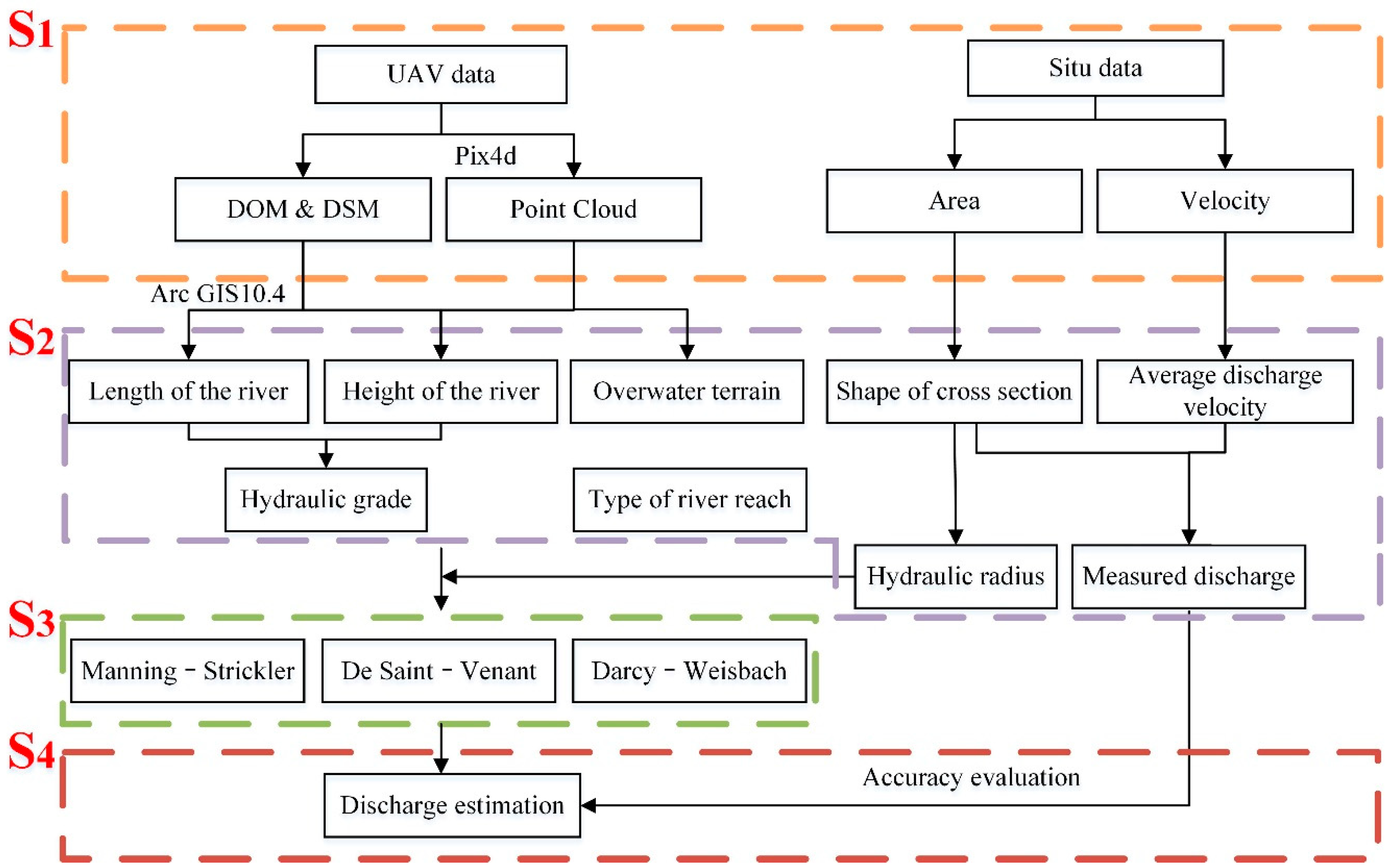
The proposed method uses four steps to calculate the river discharge in ungauged catchments (Figure 1). First, UAV data is acquired to obtain DOM and DSM (an in situ experiment is performed to obtain authentication data). Both of these are basic datasets for discharge estimation. Second, key parameters are extracted using the selected slope–area method. Detailed elevation data and rich color data are recorded in the DSM and DOM, respectively; they are used to calculate parameter values. Third, discharge is estimated using a different slope–area method. Fourth, estimated discharge is evaluated by measured discharge; the applicability of the four algorithms is compared under different river discharge scenarios.
2.1. Study Area
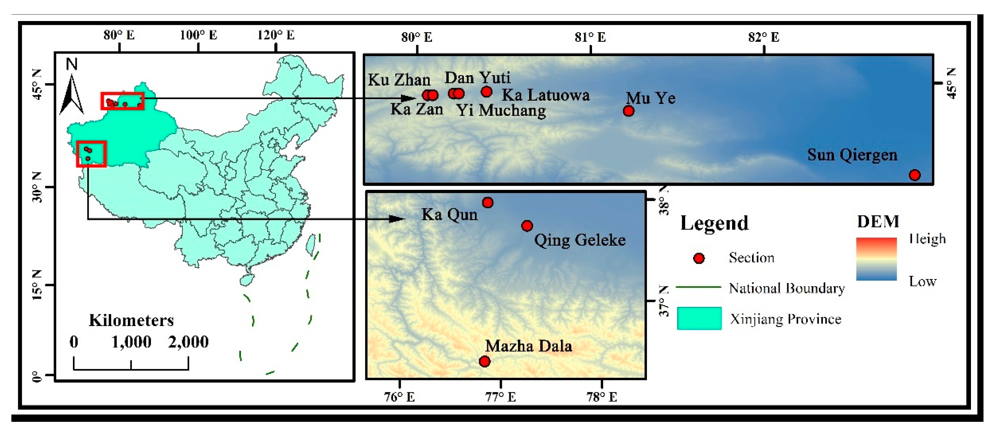
In this study, we chose ten representative sections in the northern Tibet Plateau and Dzungaria Basin, Xinjiang province, a major province in northwestern China. These areas are located upstream of the larger oases or cities, containing 71% of Xinjiang’s population (over 10 million people, https://www.xinjiang.gov.cn). Water resources are the main shortcomings that restrict the development of industry and agriculture. Ka Qun (KQ), Mazha Dala (MD), and Qing Geleke (QG) rivers all originate in the northern Tibetan Plateau. Ku Zhan (KZ), Ka Zan (KZan), Dan Yuti (DY), Yi Muchang (YM), Ka Latuowa (KL), Sun Qiergen (SQ), and Mu Ye (MY) rivers originate at the northern foot of the Tian Shan and southern foot of the Altai Mountains. The highest and lowest altitudes are 3844.2 m (MD) and 416.4 m (SQ), respectively, with an average elevation of 2061.4 m. The location of the study area is shown in Figure 2. Economic constraints and harsh natural conditions mean that hydrological data are scarce in northwest China, and human–water conflicts are getting worse. As an essential part of the Asian Water Tower, the water resources in northwest China are related to the global climate and biodiversity in arid areas [39,40].
2.2. Data
2.2.1. UAV Data
Rotary-wing UAV was used to collect topographic information about the rivers in the study area. Manufactured by DJ-Innovations (Shenzhen, China), the PHANTOM 4 UAV has four motors; it carries a camera with three visible bands (blue, green, and red). The UAV is GPS-equipped; horizontal and vertical coordinates can be recorded via the camera. It can fly for a maximum of 30 min, even in high altitude areas. When the flying height is 50–200 m, it can also collect high-resolution images. Our previous study has verified the spatial resolution and elevation resolution of the UAV data. The average error in the horizontal direction is ±0.51 cm and in the vertical direction is ±4.39 cm. The Root Mean Square Error (RMSE) in the horizontal direction is ±2.79 cm and in the vertical direction is ±9.98 cm. Overall, the measurement accuracy of the PHANTOM 4 under the professional control software is centimeter-grade [41]. In this study, we used the same equipment and data processing methods to obtain section information.
Land surface area scanned by UAV has a positive correlation with flight time, and flight time is limited by battery capacity. Obtaining sufficient data within the limited flight time is the primary problem. Therefore, we selected different flying heights according to specific conditions for each section to obtain useful data within the limited battery capacity timeframe. For example, the area where KQ, MD, QG, and SQ rivers are located is large, and the flying height is 120 m. The terrain is open and flat in the KZ, KZan, DY, YM, and KL river sections, and the flying height is 50 m. The MY river section is somewhat peculiar as its eastern flank is a steep hillside. Thus, to prevent the UAV from hitting the mountains, we set the flight height to 150 m. Specific flight control system information is presented in Table 1.
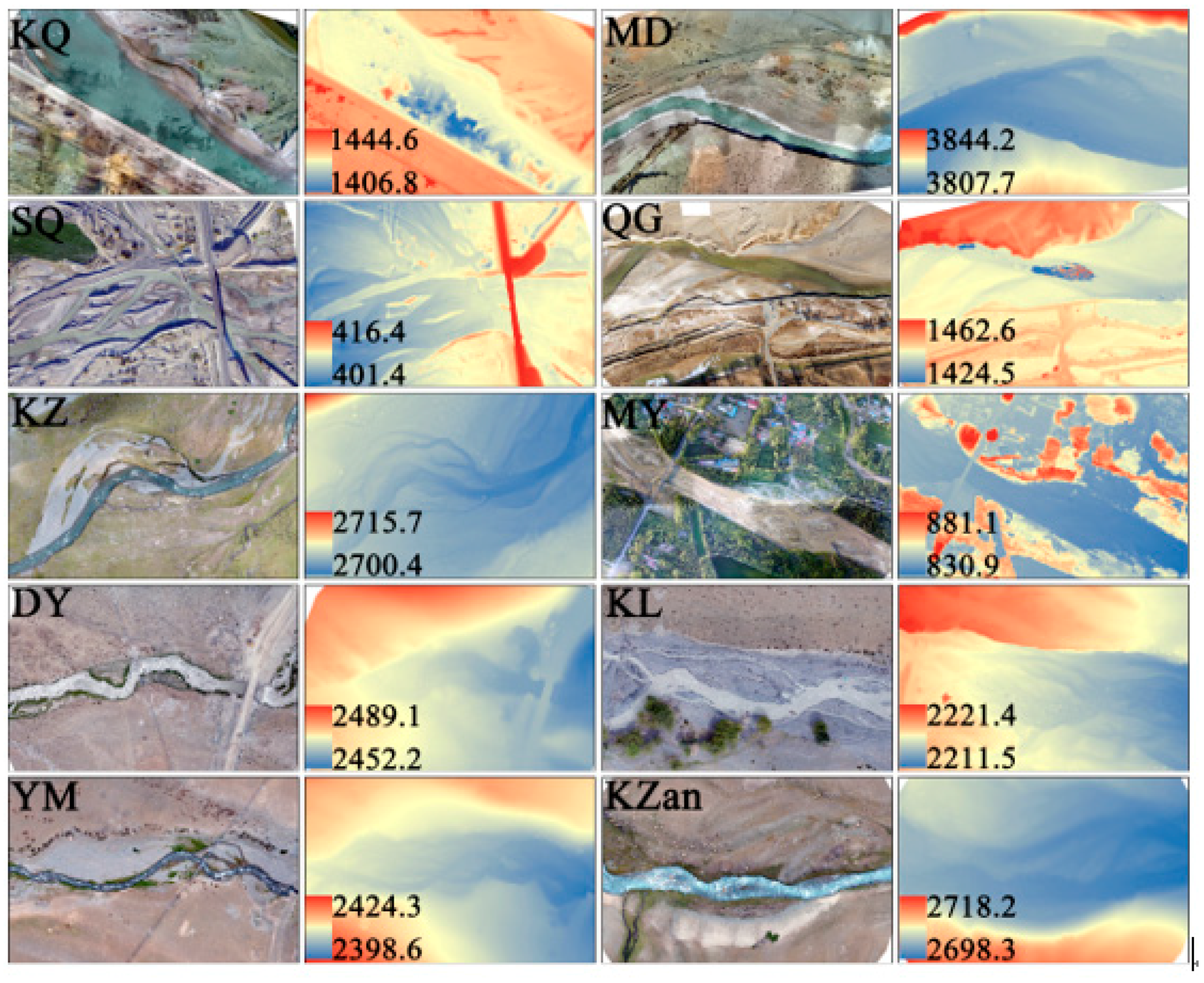
The original UAV data are JPEG pictures with geographic information, obtained using Pix4D (https://www.pix4d.com), which is a professional software application for planning flight paths in the UAV control system and splicing UAV photos to DOM and DSM using a computer. DOM records the color information (RGB) and DSM records the high-precision terrain information of the study area (Figure 3). In this study, DOM is used to classify river sections, analyze the environment of the riverbed and vegetation growth in the beach, and identify the type of river and boundaries between water and the embankment. DSM is used to calculate the hydraulic radius and hydraulic gradient. Moreover, the DSM reflected terrain changes in the region, including the elevation of embankments, roads, bridges (KQ, SQ, MY, and DY), and residential houses (MY).
2.2.2. In Situ Experimental Data
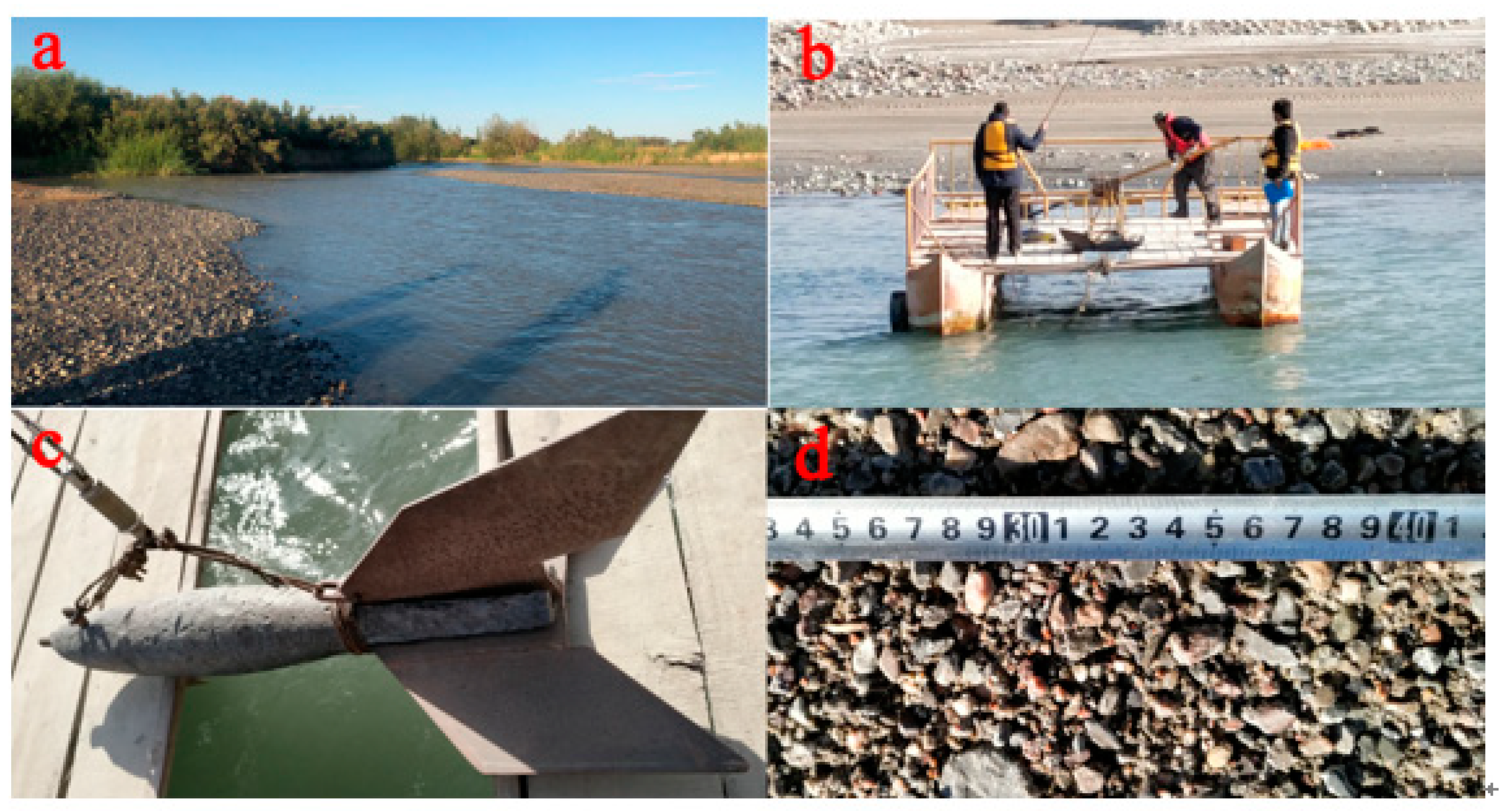
In situ experimental data is used to obtain additional data and validate the calculated result using the hydrological formula. When we collected topographic information using the UAV, we measured the discharge velocity and cross-sectional shape (area), while simultaneously recording the surrounding environment, river type, and riverbed pebble particle size information (Figure 4). Figure 4a shows landscape pictures of a river in the study area. This is representative of most rivers in our study area; they have a gravel beach and some river banks are covered with shrubs. Figure 4b shows workers measuring the cross-sectional data in a survey boat. Survey boats were used to measure in situ data where the river depth exceeded 2 m. Figure 4c shows a lead fish, which was used in the in situ experiments to measure the cross-section and flow rate. Instruments for discharge velocity measurement are suspended from it. Figure 4d illustrates the changes in pebble particle size along the riverbank; this is used to analyze the roughness in different rivers. In this way, we recorded detailed in situ experiment data, including the vegetation growth state, the particle size of pebbles, and geographical characteristics of river sections.
Discharge velocity and cross-sectional shape are obtained using the velocity–area method, which is based on an integral algorithm widely used to determine the average discharge velocity and water depth [26]. We set up regular measurement lines along the cross-section of a river. The measured discharge velocity at 60% of the water depth is used to determine the average discharge velocity. Table 2 presents information about the section, date, and average discharge velocity. Except YM and MY sections, all the velocities are above 1 m/s, as they are mountainous rivers. The maximum velocity is 2.3 m/s in DY section, and the average velocity over the ten sections is 1.38 m/s, which is faster than in a typical non-mountainous river.
2.3. Hydraulic Algorithms
As typical algorithms of the slope–area method, the Manning–Strickler formula (M–S), Saint-Venant system of equivalence (S-V), and Darcy–Weisbach equivalence (D–W) are widely used to calculate river discharge and water conservation potential [36,42,43].
M–S is an empirical formula that is typically used to estimate the average discharge of a channel or conduit that is not entirely enclosed. It has a specific physical principle and relatively simple calculation process; it is widely used in basic calculations. The classical M–S can be written as [35,44]:
where is the average velocity, m/s; is a conversion factor, m1/3/s (set to 1 in this study); is the roughness or Gauckler–Manning coefficient, which is a dimensionless indicator of the roughness coefficient in the river course; is the hydraulic radius, which depends on the cross-sectional shape; and is the hydraulic gradient, which is used to describe the slope of the vertical section.
The river discharge is formally given by the following equation:
where is the channel discharge, m3/s; is the cross-sectional area, m2.
Saint-Venant first proposed his system of equations in 1871. S-V is often used to describe the law of motion of water that has a free surface. The continuous equation reflects the law of conservation of mass (Equation (3)) and a motion equation reflecting the law of conservation of momentum (Equation (4)) [45,46]:
where is the cross-sectional area, m2; t is time, s; is the river discharge, m3/s; is the distance along the river, m; is the water level, m; is the average velocity of the cross-section, m/s; g is gravitational acceleration, m/s2; and is the friction slope.
In practical applications, the item representing inertia () can be neglected (it has a value of ~1% in steady discharge). Thus, Equation (4) can be simplified to:
where is the discharge modulus; is the depth of water, . The discharge modulus is given by:
where is Chezy’s coefficient.
In natural rivers, the state of the water discharge is mostly turbulent. For such situations, we have two ways to compute the value of , namely S-V-1 and S-V-2:
S-V-1:
S-V-2:
D–W is a phenomenological equation in hydromechanics. The formula was originally used to study the discharge of water in pipes but can also be used in rivers following certain improvements. D–W expresses shear stress () between the water and the bank as follows [47]:
where is the friction coefficient; is density, kg/m3; and is the average velocity of the cross-section, m/s.
From Equation (10), the relationship between the friction coefficient and speed can be written as:
Thus, the channel discharge is formally given by:
where is gravitational acceleration m/s2; is the hydraulic radius; is the hydraulic gradient; and is the cross-sectional area, m2.
The friction coefficient can then be written as:
where is the equivalent roughness of the river.
According to the mentioned methods, nine key parameters are necessary for discharge estimation (Table 3). In this study, these parameters were obtained in three ways. The area, length of the vertical section, and hydraulic gradient were captured by UAV; the equivalent roughness and roughness are empirical parameters, and their values were taken from statistical tables; the hydraulic radius, roughness coefficient, Chezy’s coefficient, and discharge modulus are intermediate parameters.
2.4. Evaluation Method and Parameter Sensitivity Analysis
2.4.1. Evaluation Method
To assess the accuracy of discharge calculated by UAV data, we utilized two metrics. The relative accuracy reflects the accuracy of individual calculation results, and the Nash–Sutcliffe efficiency coefficient (NSE) verifies the integral quality of runoff simulation results [42].
The relative accuracy is the percentage of the absolute error in the measured value. According to existing research results, we set the threshold for the relative accuracy to 20% [48]. When the relative efficiency is less than 20%, the results are considered reliable; relative accuracy values above 20% are unreliable. NSE is an essential index for evaluating the effect of simulation calculations; values closer to 1.0 imply better simulation results. These metrics are calculated as:
where is the calculated discharge, is the measured discharge, and is the number of simulation calculations.
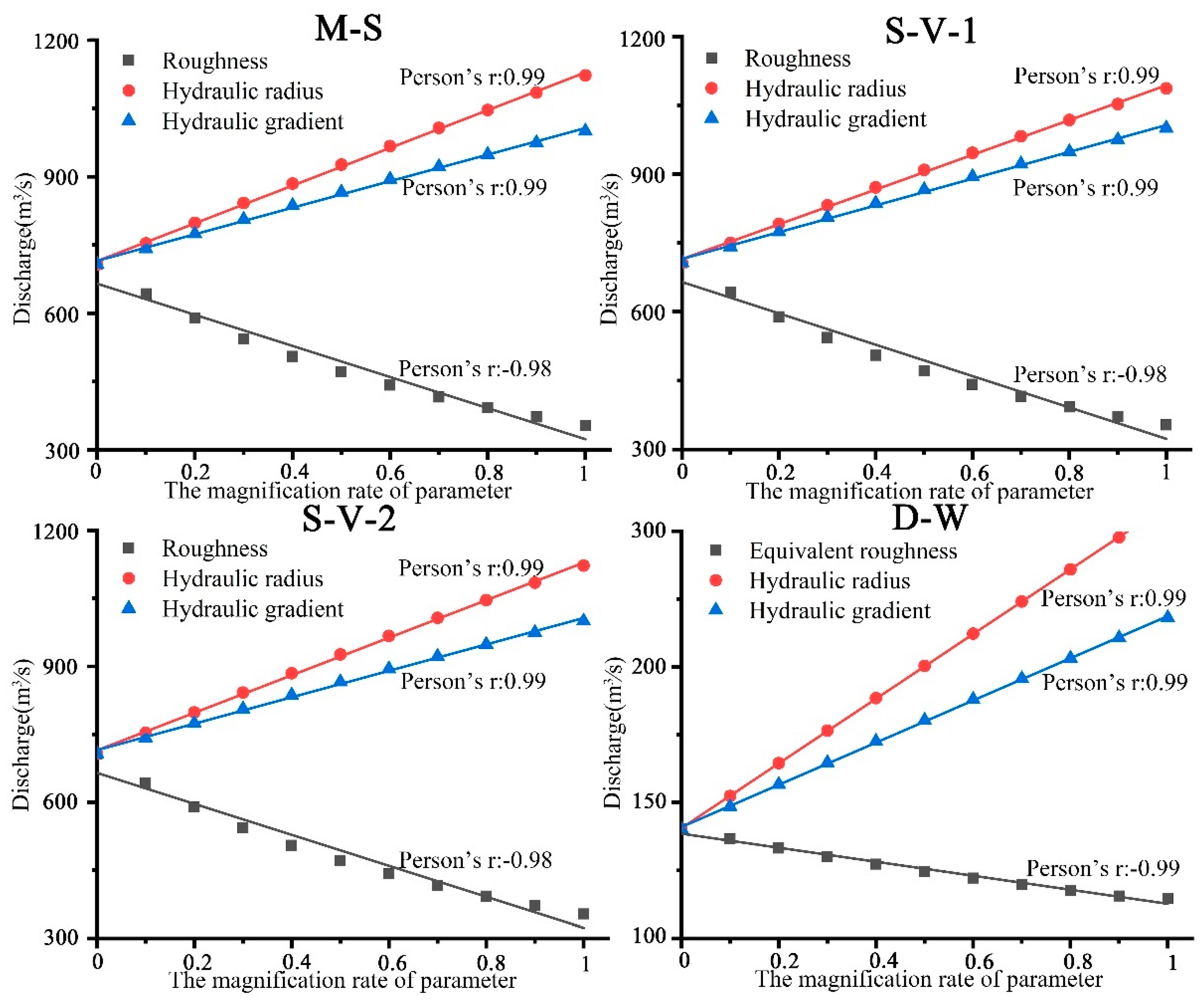
2.4.2. Parameter Sensitivity Analysis
There are nine parameters for M–S, S-V, and D–W; it is crucial to determine which is the most important. To analyze the influence of each parameter on the calculated discharge, we selected the roughness, hydraulic gradient, hydraulic radius for M–S and S-V, and the equivalent roughness, hydraulic gradient, and hydraulic radius for D–W as key parameters to be verified. The initial values of the roughness, equivalent roughness, hydraulic gradient, and hydraulic radius were set to 0.01, 0.30, 1.00, and 0.005, respectively. The area was set to 100 m2 (constant). The control variates method was applied to ensure that most of the actual parameters were within the range of variation. Holding the other parameters fixed, we repeatedly increased the initial value of the target parameter by 10% until it was twice the initial value.
3. Results
3.1. Preprocessing and Critical Parameter Results
River morphology parameters such as the hydraulic gradient, cross-sectional area, wetted perimeter, and hydraulic radius are necessary for discharge estimation. The vertical section, which shows the variation of elevation with distance, was used to calculate the hydraulic gradient. The area, wetted perimeter, and hydraulic radius were calculated in the cross-section.
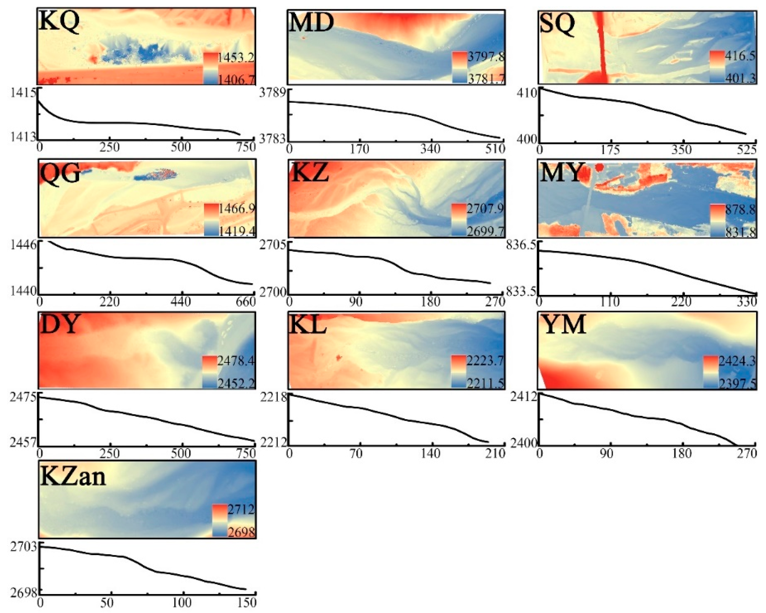
Detailed topographic information and abundant surface information were recorded in the DSM and DOM derived from the UAV images. This information was used to determine the variation of the elevation in the vertical section. The 3D Analyst tool in ArcGIS 10.4 was used to measure minor elevation changes and determine the vertical section of the river. Figure 5 shows the DSM of the study river and the shape of the vertical section. Bridges, roads, and other river-crossing structures appear in the partial study area (SQ, MY, DY, and KL). DSM also recorded their elevation information as interference information for the vertical section. In this study, the width is small relative to the vertical section of the river. When such interferences were encountered, we interrupted the measurement and supplemented the missing part using interpolation. Note that KQ is a concave curve and the others are convex or gentle. The field observations showed that the riverbank of KQ is cement-modified for an agricultural water diversion facility downstream. Only KQ shows evidence of such human management, whereas the other sections exist in their natural state.
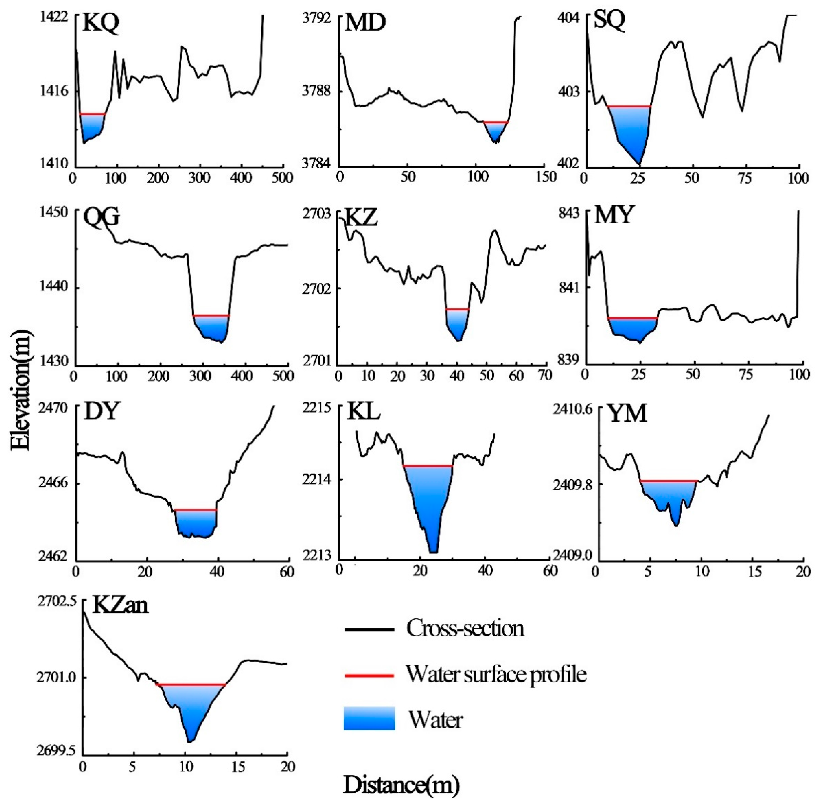
The monitoring section was selected in the middle of the flight area, ensuring that the distance between the upstream and downstream parts was approximately equal. However, the influence of the water body on the elevation measurements cannot be ignored [49]. The detailed underwater terrain still requires in situ data. We divided the cross-sections into two parts: below the water surface and above the water surface. For the section under the water surface, the terrain data obtained from the UAV were measured manually (Section 2.2.2). This is particularly helpful in the case of braided rivers and for estimating river-wide discharges (Figure 6). All sections are triangular or trapezoidal. Some cross-sections are similar to rectangles because of the difference in the ratio of horizontal and vertical coordinates, such as in the QG, KZ, and DY sections. These sections are located in the mountains, where triangles and trapezoids are the normal shapes.
Based on the vertical sections (Figure 5) and cross-sections (Figure 6), the hydraulic gradient in the vertical section, the area, and hydraulic radius in the cross-section were computed (Table 4). These rivers are located in mountainous areas and the parameter values were higher than those for normal rivers. The maximum value of the hydraulic gradient was 0.068 (DY) and the average value was 0.024. Our research targets are medium and small size rivers, which have small cross-sectional areas, triggering the difference in area classification. In all sections, the maximum value was 92.56 m2 (KQ) and the average was 20.98 m2. Eight-tenths of the cross-sectional area was less than 20 m2. The hydraulic radius characterizes the water transport capacity of a section. The sections in this study can be generalized into triangles or trapezoids, and the value of the hydraulic radius is similar to that in narrow-deep rivers.
3.2. Results of the Key Parameters and the River Discharge
The key parameters used in the discharge calculations were obtained from UAV data and in situ experiments (Table 5). KZan, DY, and YM sections were close to their sources; however, the basin terrain data changes drastically. The values of J in these sections were relatively larger than others. Because of gravel in KZan, DY, and YM sections, they had the maximum values of roughness (n) and equivalent roughness (Δ). Other sections are at the midstream (exit position of the valley) or downstream sections of the river, hence J was smooth, and n and Δ showed medium values. Overall, the parameters of all ten sections were different from those of rivers in the plains.
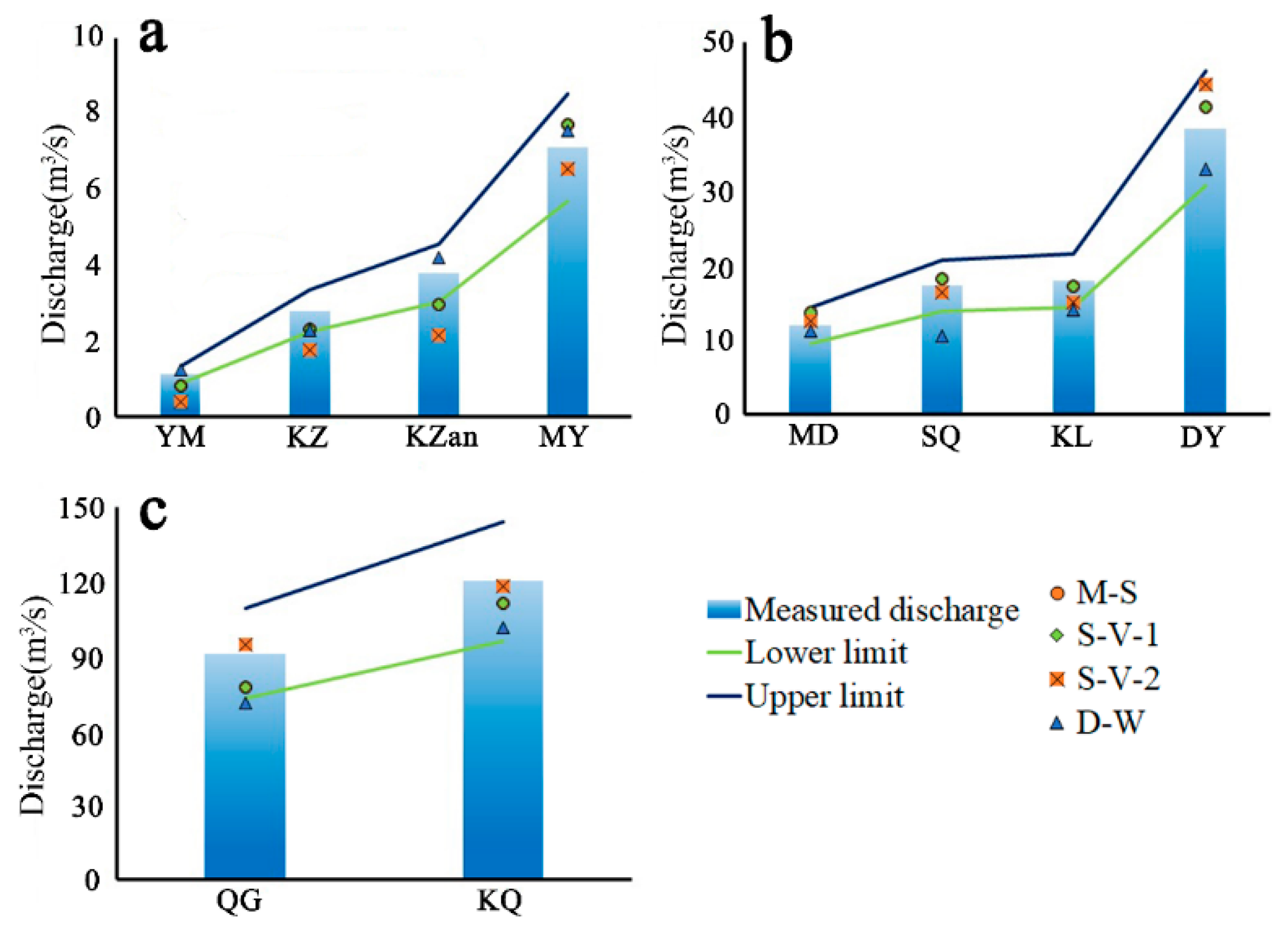
The discharges calculated using M–S, S-V-1, S-V-2, D–W, and the limit of relative accuracy are presented in Figure 7. To describe the differences, we have divided the results into three parts based on the discharge level: <10 m3⁄s (Figure 7a), 10–50 m3⁄s (Figure 7b), and >50 m3⁄s (Figure 7c). The results given by M–S are consistent with S-V-1 because both M–S and S-V-1 are derived from Chezy’s equation, which is another classical hydrological formula. However, the different equation transformations produce a somewhat different appearance. To illustrate the various calculation methodologies and the complicated relationship among hydrological calculation methods, M–S and S-V-1 are considered as different methods.
3.3. Validation of the Estimated River Discharges
The discharges measured from in situ experiments were regarded as the true values for validating the estimated river discharges. The relative accuracy of M–S, S-V, D–W, and the measured discharge of ten sections are shown in Figure 7. The overall qualification rate of the discharge calculation method based on UAV data was 70%, with 28 successful calculations and 12 failed calculations. Between these classical methods, when the discharges were greater than 10 m3⁄s, the D–W method produced an underestimation in KQ, MD, QG, KZan, YM, and SQ sections. Further, when the discharge was greater than 20 m3⁄s, S-V-2 produced an overestimation in KQ, QG, KZan, and YM sections. M–S and S-V-1 were usually at a medium level. These conclusions were only observed at different discharge levels as different methods have their own characteristics.
Considering the average relative accuracy, the results in all sections are acceptable, except KZ, KZan, and YM. The most significant error was found for the YM section; the average error was 0.35 m3/s, approximately one-third of the measured value. KZ and KZan were in similar situations; their average errors were 0.64 m3/s and 1.11 m3/s, respectively. The measured discharges in KZ, KZan, and YM were less than 5 m3/s. When we set 20% as the evaluation standard, the permitted error was ±1 m3/s, producing a narrow range of acceptable discharges. This is somewhat strict for an empirical formula. The discharge was greater than 5 m3/s in the other seven sections, and the average error in the calculated discharge was within an acceptable limit. Because of the larger margin of error, the calculated discharge varied more widely. For example, in KQ, the measured favorable was 120.33 m3/s and the error in S-V-2 was 1.98 m3/s, which was larger than in KZ, KZan, and YM sections. However, the relative accuracy was 1.64%, the smallest of all the results.
Table 6 shows the NSE of M–S, S-V-1, S-V-2, and D–W. The value of NSE was greater than 0.90 and the average was 0.98. The S-V-2 gave the best NSE value of the four methods. The high values of the NSE meant that calculating river discharge with UAV data was useful. Conventional techniques combined with UAV data have excellent adaptability in the northern Tibet Plateau and Dzungaria Basin.
3.4. Performance of the Methods with Different Discharge Levels
To describe the accuracy of the four methods with respect to the river discharge level, we divided the calculated results into three classes according to the measured discharge. These classes are less than 10 m3⁄s, 10–50 m3⁄s, and greater than 50 m3⁄s, representing low, medium, and high discharges, respectively, in small- and medium-sized rivers (Table 7). The four methods exhibited different advantages at different discharge levels.
There were four sections where the measured river discharges were less than 10 m3⁄s (KZ: 2.80 m3⁄s, KZan: 4.15 m3⁄s, YM: 1.11 m3⁄s, and MY: 7.11 m3⁄s), representing low-discharge rivers. D–W achieved better performance than the other methods (Figure 7a). The average relative accuracy of the four sections was 9.41%, less than the 20% threshold. Thus, we recommend D–W as the discharge calculation formula for small rivers when the discharge level is less than 10 m3/s.
Four sections were classified as having a medium discharge level (MD: 15.14 m3⁄s, DY: 38.44 m3⁄s, KL: 18.92 m3⁄s, and SQ: 17.26 m3⁄s). The M–S and S-V-1 methods offered the best performance for this river class, with an average relative accuracy of 7.95% (Figure 7b). When the discharge was between 10 m3⁄s and 50 m3⁄s, M–S and S-V-1 were better than other methods.
The third discharge level includes KQ (120.33 m3⁄s) and QG (91.08 m3⁄s). Compared to the other methods, S-V-2 was the best performer in calculating the discharge of large-flow rivers. The average relative accuracy of S-V-2 for these two sections was 2.74% (Figure 7c), the calculated results were very close to the measured values.
4. Discussion
4.1. Parameters that Most Influence the Final Results
When the discharge and magnification rate of parameters are plotted together, there exists an apparent linear relationship between the discharges and parameters (Figure 8). Hence, the key parameter can be selected by examining the slopes of the fitting lines. The results show that Pearson’s correlation coefficient (Pearson’s r) for the fitting equation is greater than 0.98, suggesting that fitting the data series using a linear equation is reliable. The variations in the parameters could significantly influence the estimated discharge. Thus, it is feasible to judge the influence of each parameter on the discharge by the absolute value of the slope of the fitting equation.
Analyzing the absolute value of the slope shows that the hydraulic radius is a significant factor in the control variables. The hydraulic radius is calculated using the wetted perimeter and area, indicating the size of the water-carrying capacity of the section. The hydraulic radius is also related to the water depth, water surface width, and cross-sectional shape [50]. According to the parameter sensitivity analysis and this theoretical basis, we believe that the hydraulic radius represents the shape of the cross-section and is an essential index for determining the water-carrying capability. The area and wetted perimeter are the basic parameters related to the hydraulic radius, both of which can be obtained from the cross-section [43,51,52].
4.2. Role of Prior Knowledge and Human Influence on this New Method
Among the nine parameters necessary for discharge estimation (Table 3), only the roughness (n) and equivalent roughness (Δ) parameters depend on prior knowledge. In this study, their values were obtained from long-term observations by local hydrological workers; the values of these two parameters are reasonable. In previous studies, roughness and equivalent roughness were not fixed but were calculated as a function of the discharge conditions [53,54,55,56]. Roughness and equivalent roughness are related to the river type, sediment particle size, slope protection, and vegetation condition [57,58]. During the design and construction of many hydraulic engineering projects, their values were typically obtained through experiments [59]. However, natural rivers are more complicated than artificial engineering scenarios. When the river is at different stages of development, various geographical environments or human disturbances have a significant impact on roughness and equivalent roughness [26]. This is the main factor limiting the growth of the present study.
Human influences that have changed the natural water cycle also affected the accuracy of our method. The discharge level will increase with the watershed area [60,61,62], as a larger watershed collects more precipitation. However, this condition is inaccurate when the influence of human activities is considered, such as dams, diversion channels, and industrial and agricultural wastewater. In this study, the discharge level did not match the watershed area. Water resources are relatively scarce in Xinjiang because of its continental climate; diversion channels have been constructed to divert the limited water resources for agricultural development, but these obstruct the water balance of a river. Hence, in the watersheds where human activities are intense, discharge levels do not correspond to the associated watershed area [63,64].
4.3. Leading Role of UAV Remote Sensing and its Limitations
The relative accuracy and NSE used as evaluation metrics in this study are both positive, proving that the UAV data are being used effectively in the proposed method. Many previous studies have elaborated on the application of UAV in discharge estimation [65,66]. Compared with professional measuring instruments, UAV monitoring is usually low-cost. It is helpful to overcome the limitations of financial and data return methods. UAV monitoring also makes it possible for scientists to design their own programs or sensors [67]. The flexibility and accuracy of UAV data make UAV potent tools for topographic surveys, which are essential components of discharge estimation. UAV monitoring represents an efficient means of obtaining topographic information, especially in ungauged catchments. High-precision data include more detail, helping researchers obtain more useful information. Simple operations and automatic processing methods reduce the temporal cost of information collection. UAV should be applied in the field of hydrological information acquisition because of their flexibility, simplicity, and speed, especially in relation to river discharges. Previous studies have shown that many rough observations may result in better data compared with few accurate experiments [68,69]. UAV, as a kind of low-cost equipment, can obtain information simply and quickly. UAV have the basic conditions to carry out a large number of observations and the advantage of application in different scenes.
Although vital to the method proposed in this study, UAV still have some limitations. For instance, it is difficult to use UAV to obtain underwater topographic information, such as the shape of the cross-section and vertical section of the river channel. At present, most UAV sensors have insufficient penetration in water, especially silt-carrying discharge [49]. This scenario still requires manual assistance, hence automatic measurement and calculation cannot be realized. This is a crucial limitation of the UAV remote sensing technique developed in this study.
5. Conclusions
To resolve the problem of river discharge monitoring in ungauged catchments, this study combined four methods based on the classical slope–area method with UAV remote sensing. The parameters of each method were retrieved from UAV images. The relative accuracy and NSE between the calculated and measured discharges were qualified. This means that the proposed method is suitable for monitoring river discharges in ungauged catchments. The selected methods were compared to find the most suitable discharge model at different discharge levels. We found that when the discharge was less than 10 m3⁄s, D–W was the most appropriate method, and when the discharge was between 10 m3⁄s and 50 m3⁄s, M–S or S-V-1 are recommended. Finally, when the discharge was greater than 50 m3⁄s, S-V-2 should be employed. This research has demonstrated the advantages of using UAV data, as it is suitable for river discharge estimations, thus expanding the research results of PUB. The proposed approach offers a new method for obtaining and analyzing discharge information over widespread areas, for which there are insufficient hydrological data.
Author Contributions
Conceptualization S.Y., P.W., J.W., H.L.; Methodology P.W., J.W.; Software P.W., H.L., J.W.; Supervision S.Y., C.Z.; Project administration T.G.; Visualization P.W., J.W.; Writing-original draft preparation P.W., H.L., J.W.
Funding
This research was funded by the National Natural Science Foundation of China grant number (U1812401, 41801334, U1603241), the China Postdoctoral Science Foundation grant number (2017M620663).
Acknowledgments
The authors thank the Tibet Water Resources Department and National Natural Science Foundation of China, and are grateful for the financial support received from the China Postdoctoral Science Foundation.
Conflicts of Interest
The authors declare no conflict of interest.
References
- Ramanathan, V.; Terborgh, J.; Lopez, L.; Núñez, P.; Rao, M.; Shahabuddin, G.; Orihuela, G.; Riveros, M.; Ascanio, R.; Adler, G.H.; et al. Aerosols, Climate, and the Hydrological Cycle. Science 2001, 294, 2119–2124. [Google Scholar] [CrossRef] [PubMed]
- DeAngelis, A.M.; Qu, X.; Zelinka, M.D.; Hall, A. An observational radiative constraint on hydrologic cycle intensification. Nature 2015, 528, 249–253. [Google Scholar] [CrossRef] [PubMed]
- Li, Y.; Piao, S.; Li, L.Z.X.; Chen, A.; Wang, X.; Ciais, P.; Huang, L.; Lian, X.; Peng, S.; Zeng, Z.; et al. Divergent hydrological response to large-scale afforestation and vegetation greening in China. Sci. Adv. 2018, 4, eaar4182. [Google Scholar] [CrossRef] [PubMed]
- Rui, X. Hydrology Princiole; China Water&Power Press: Beijing, China, 2004. [Google Scholar]
- Yang, S. Ecohydrological Models: Introduction and Application; Science Press: Beijing, China, 2012. [Google Scholar]
- Ji, M.; Huang, J. Global Semi-Arid Climate Change over Last 60 Years. Clim. Dyn. 2016, 46, 1131–1150. [Google Scholar]
- Bjerklie, D.M.; Moller, D.; Smith, L.C.; Dingman, S.L. Estimating discharge in rivers using remotely sensed hydraulic information. J. Hydrol. 2005, 309, 191–209. [Google Scholar] [CrossRef]
- Vörösmarty, C.J.; McIntyre, P.B.; Gessner, M.O.; Dudgeon, D.; Prusevich, A.; Green, P.; Glidden, S.; Bunn, S.E.; Sullivan, C.A.; Liermann, C.R.; et al. Global threats to human water security and river biodiversity. Nature 2010, 467, 555–561. [Google Scholar] [CrossRef] [PubMed]
- Sivapalan, M.; Takeuchi, K.; Franks, S.W.; Gupta, V.K.; Karambiri, H.; Lakshmi, V.; Liang, X.; Mcdonnell, J.J.; Mendiondo, E.M.; O’Connell, P.E. IAHS Decade on Predictions in Ungauged Basins (PUB), 2003–2012: Shaping an exciting future for the hydrological sciences. Int. Assoc. Sci. Hydrol. Bull. 2003, 48, 857–880. [Google Scholar] [CrossRef]
- Jones, D.A.; Kay, A.L. Uncertainty analysis for estimating flood frequencies for ungauged catchments using rainfall-runoff models. Adv. Water Resour. 2007, 30, 1190–1204. [Google Scholar] [CrossRef]
- Yadav, M.; Wagener, T.; Gupta, H. Regionalization of constraints on expected watershed response behavior for improved predictions in ungauged basins. Adv. Water Resour. 2007, 30, 1756–1774. [Google Scholar] [CrossRef]
- Pappenberger, F.; Beven, K.J.; Ratto, M.; Matgen, P. Multi-method global sensitivity analysis of flood inundation models. Adv. Water Resour. 2008, 31, 1–14. [Google Scholar] [CrossRef]
- Oudin, L.; Andréassian, V.; Perrin, C.; Michel, C.; Le Moine, N. Spatial proximity, physical similarity, regression and ungaged catchments: A comparison of regionalization approaches based on 913 French catchments. Water Resour. Res. 2008, 44, 893–897. [Google Scholar] [CrossRef]
- Bao, Z.; Zhang, J.; Liu, J.; Fu, G.; Wang, G.; He, R.; Yan, X.; Jin, J.; Liu, H. Comparison of regionalization approaches based on regression and similarity for predictions in ungauged catchments under multiple hydro-climatic conditions. J. Hydrol. 2012, 466, 37–46. [Google Scholar] [CrossRef]
- Cheng, C.; Ou, C.; Chau, K.W. Combining a fuzzy optimal model with a genetic algorithm to solve multi-objective rainfall–runoff model calibration. J. Hydrol. 2002, 268, 72–86. [Google Scholar] [CrossRef]
- Gassman, P.W.; Reyes, M.R.; Green, C.H.; Arnold, J.G. The Soil and Water Assessment Tool: Historical Development, Applications, and Future Research Directions. Trans. ASABE 2007, 50, 1211–1250. [Google Scholar] [CrossRef]
- Madsen, H. Automatic calibration of a conceptual rainfall–runoff model using multiple objectives. J. Hydrol. 2000, 235, 276–288. [Google Scholar] [CrossRef]
- Ratto, M.; Pagano, A.; Young, P. State Dependent Parameter metamodelling and sensitivity analysis. Comput. Phys. Commun. 2007, 177, 863–876. [Google Scholar] [CrossRef]
- Wagener, T.; Sivapalan, M.; Troch, P.; Woods, R. Catchment Classification and Hydrologic Similarity. Geogr. Compass 2007, 1, 901–931. [Google Scholar] [CrossRef]
- Neal, J.; Schumann, G.; Bates, P.; Buytaert, W.; Matgen, P.; Pappenberger, F. A data assimilation approach to discharge estimation from space. Hydrol. Process. 2009, 23, 3641–3649. [Google Scholar] [CrossRef]
- Ling, F.; Cai, X.; Li, W.; Xiao, F.; Li, X.; Du, Y. Monitoring river discharge with remotely sensed imagery using river island area as an indicator. J. Appl. Remote Sens. 2012, 6, 063564. [Google Scholar] [CrossRef]
- Huang, J.; Li, Y.; Fu, C.; Chen, F.; Fu, Q.; Dai, A.; Shinoda, M.; Ma, Z.; Guo, W.; Li, Z.; et al. Dryland climate change: Recent progress and challenges. Rev. Geophys. 2017, 55, 719–778. [Google Scholar] [CrossRef]
- Bjerklie, D.M.; Ayotte, J.D.; Cahillane, M.J. Simulating Hydrologic Response to Climate Change Scenarios in Four Selected Watersheds of New Hampshire; US Geological Survey Scientific Investigations Report: Reston, VA, USA, 2015.
- Gleason, C.; Garambois, P.; Durand, M.J.E. Tracking river flows from space. EOS 2017, 98. [Google Scholar] [CrossRef]
- Gleason, C.J.; Smith, L.C. Toward global mapping of river discharge using satellite images and at-many-stations hydraulic geometry. Proc. Natl. Acad. Sci. USA 2014, 111, 4788–4791. [Google Scholar] [CrossRef] [PubMed]
- Huang, Q.; Long, D.; Du, M.; Zeng, C.; Qiao, G.; Li, X.; Hou, A.; Hong, Y. Discharge estimation in high-mountain regions with improved methods using multisource remote sensing: A case study of the Upper Brahmaputra River. Remote Sens. Environ. 2018, 219, 115–134. [Google Scholar] [CrossRef]
- Xiang, H.; Tian, L.J.B. Development of a low-cost agricultural remote sensingsystem based on an autonomous unmanned aerial vehicle (UAV). Biosyst. Eng. 2011, 108, 174–190. [Google Scholar] [CrossRef]
- Neitzel, F.; Klonowski, J. Mobile 3d mapping with a low-cost uav system. ISPRS Int. Arch. Photogramm. Remote Sens. Spat. Inf. Sci. 2012, 39–44. [Google Scholar] [CrossRef]
- Harder, P.; Schirmer, M.; Pomeroy, J.; Helgason, W. Accuracy of snow depth estimation in mountain and prairie environments by an unmanned aerial vehicle. Cryosphere 2016, 10, 2559–2571. [Google Scholar] [CrossRef]
- Dewitt, B.A.; Wolf, P.R. Elements of Photogrammetry (with Applications in GIS); McGraw-Hill: New York, NY, USA, 2000. [Google Scholar]
- Forsmoo, J.; Anderson, K.; MacLeod, C.J.A.; Wilkinson, M.E.; Brazier, R. Drone-based structure-from-motion photogrammetry captures grassland sward height variability. J. Appl. Ecol. 2018, 55, 2587–2599. [Google Scholar] [CrossRef]
- Zhao, C.; Zhang, C.; Yang, S.; Liu, C.; Xiang, H.; Sun, Y.; Yang, Z.; Zhang, Y.; Yu, X.; Shao, N.; et al. Calculating e-flow using UAV and ground monitoring. J. Hydrol. 2017, 552, 351–365. [Google Scholar] [CrossRef]
- Lewin, J.; Gibbard, P. Quaternary river terraces in England: Forms, sediments and processes. Geomorphology 2010, 120, 293–311. [Google Scholar] [CrossRef]
- Riggs, H. A simplified slope-area method for estimating flood discharges in natural channels. J. Res. US Geol. Surv. 1976, 4, 285–291. [Google Scholar]
- Dingman, S.; Sharma, K.P. Statistical development and validation of discharge equations for natural channels. J. Hydrol. 1997, 199, 13–35. [Google Scholar] [CrossRef]
- Sikder, M.S.; Hossain, F. Understanding the Geophysical Sources of Uncertainty for Satellite Interferometric (SRTM)-Based Discharge Estimation in River Deltas: The Case for Bangladesh. IEEE J. Sel. Top. Appl. Earth Obs. Remote Sens. 2015, 8, 523–538. [Google Scholar] [CrossRef]
- Stewart, A.M.; Callegary, J.B.; Smith, C.F.; Gupta, H.V.; Leenhouts, J.M.; Fritzinger, R.A. Use of the continuous slope-area method to estimate runoff in a network of ephemeral channels, southeast Arizona, USA. J. Hydrol. 2012, 472, 148–158. [Google Scholar] [CrossRef]
- Bjerklie, D.M.; Dingman, S.L.; Vörösmarty, C.J.; Bolster, C.H.; Congalton, R.G. Evaluating the potential for measuring river discharge from space. J. Hydrol. 2003, 278, 17–38. [Google Scholar] [CrossRef]
- Dukhovny, V.A.; Schutter, J.D. Water in Central Asia: Past, Present, Future; Crc Press: Boca Raton, FL, USA, 2011. [Google Scholar]
- Immerzeel, W.W.; Van Beek, L.P.H.; Bierkens, M.F.P. Climate Change Will Affect the Asian Water Towers. Science 2010, 328, 1382–1385. [Google Scholar] [CrossRef] [PubMed]
- Zhang, C.; Yang, S.; Zhao, C.; Lou, H.; Zhang, Y.; Bai, J.; Wang, Z.; Guan, Y.; Zhang, Y. Topographic data accuracy verification of small consumer UAV. J. Remote Sens. 2018, 22, 185–195. [Google Scholar]
- Sichangi, A.W.; Wang, L.; Yang, K.; Chen, D.; Wang, Z.; Li, X.; Zhou, J.; Liu, W.; Kuria, D. Estimating continental river basin discharges using multiple remote sensing data sets. Remote Sens. Environ. 2016, 179, 36–53. [Google Scholar] [CrossRef] [Green Version]
- Tang, H.; Yan, J.; Xiao, Y.; Lu, S.Q. Manning’s roughness coefficient of vegetated channels. J. Hydraul. Eng. 2007, 38, 1347–1353. [Google Scholar]
- Sun, D. Hydraulics; Zhengzhou University Press: Henan, China, 2007. [Google Scholar]
- Maidment, D.R. Handbook of Hydrology; McGraw-Hill: New York, NY, USA, 1993. [Google Scholar]
- Bao, W. Hydrologic Forecasting; China Water&Power Press: Beijing, China, 2006. [Google Scholar]
- Shao, X.; Wang, X. Introduction to River Mechanics; Tsinghua University Press: Beijing, China, 2005. [Google Scholar]
- Birkinshaw, S.; Moore, P.; Kilsby, C.; O’donnell, G.; Hardy, A.J.; Berry, P. Daily discharge estimation at ungauged river sites using remote sensing. Hydrol. Process. 2014, 28, 1043–1054. [Google Scholar] [CrossRef]
- Kerr, J.M.; Purkis, S. An algorithm for optically-deriving water depth from multispectral imagery in coral reef landscapes in the absence of ground-truth data. Remote. Sens. Environ. 2018, 210, 307–324. [Google Scholar] [CrossRef]
- Liu, C.; Men, B.; Song, J. Ecological Hydraulic Radius Method for Estimating Ecological Water Demand in River. Prog. Nat. Sci. 2007, 17, 42–48. [Google Scholar]
- Ree, W.O.; Palmer, V.J. Flow of Water in Channels Protected by Vegetative Linings; US Dept. of Agriculture: Washington, DC, USA, 1949.
- Jin, J.; Yang, X.; Jin, B.; Ding, J. A new method for computation of flow surface profile in open channel. J. Hydraul. Eng. 2000, 9, r28. [Google Scholar]
- Beven, K.; Binley, A. The Future of Distributed Models—Model Calibration and Uncertainty Prediction. Hydrol. Process. 2010, 6, 279–298. [Google Scholar] [CrossRef]
- Einstein, H.A. Bed-Load Transportation in Mountain Creek; United States Department of Agriculture: Washington, DC, USA, 1944. [Google Scholar]
- Hemphill, R.; Bramley, M. Protection of River and Canal Banks; China Water & Power Press: Beijing, China, 2000. [Google Scholar]
- Qian, N.; Hong, R.; Mai, Q.; Bi, C. Channel Roughness of Lower Yellow River. J. Sediment Res. 1959, 4, 34–36. [Google Scholar]
- Myers, W. Flow resistance in wide rectangular channels. J. Hydraul. Div. 1982, 108, 471–482. [Google Scholar]
- Simons, D.B.; Li, R.M.; Al-Shaikh-Ali, K.S. Flow resistance in cobble and boulder riverbeds. J. Hydraul. Div. 1979, 105, 477–488. [Google Scholar]
- Chow, V.T. Open Channel Hydraulics; McGraw-Hill: New York, NY, USA, 1959. [Google Scholar]
- Guo, X.; Chen, J.; Zou, N.; Fan, K.; Zhang, J.; Hu, Q. Research on stage-discharge relation of main hydrologic stations on middle and lower reach of the Yangtze River. Yangtze R 2006, 37, 68–71. [Google Scholar]
- Hong, Z.; Jian-Wei, W.; Qiu-Hong, Z.; Yun-Jiang, Y. A preliminary study of oasis evolution in the Tarim Basin, Xinjiang, China. J. Arid. Environ. 2003, 55, 545–553. [Google Scholar] [CrossRef]
- Chen, Y.; Xu, Z. Possible Impact of Global Climate Change on Water Resources in Tarim River Basin, Xinjiang. SCI. CH. Earth Sci. 2004, 34, 1047–1053. [Google Scholar]
- Guo, Z. Initial Analysis of Estimation for Usable Quantity of Water Resources. J. China Hydrol. 2001, 5, 23–26. [Google Scholar]
- Xu, Y. A Study of Comprehensive Evaluayion of The Water Resource Carrying Capacity in The Aeid Area—A case study in the Hetian river basin of Xinjiang. J. Nat. Resour. 1993, 8, 229–237. [Google Scholar]
- Rivas, C.M.; Ballesteros, G.R.; Thomas, K.; Amanda, V. Automated Identification of River Hydromorphological Features Using UAV High Resolution Aerial Imagery. Sensors 2015, 15, 27969–27989. [Google Scholar]
- Vidan, C.; Maracine, M. Corona Discharge Classification Based on UAV Data Acquisition. In Proceedings of the 21st International Conference on Control Systems and Computer Science (CSCS), Bucharest, Romania, 29–31 May 2017; pp. 690–695. [Google Scholar]
- Tauro, F.; Selker, J.; Van De Giesen, N.; Abrate, T.; Uijlenhoet, R.; Porfiri, M.; Manfreda, S.; Caylor, K.; Moramarco, T.; Benveniste, J.; et al. Measurements and Observations in the XXI century (MOXXI): innovation and multi-disciplinarity to sense the hydrological cycle. Hydrol. Sci. J. 2018, 63, 169–196. [Google Scholar] [CrossRef] [Green Version]
- Haberlandt, U.; Sester, M. Areal rainfall estimation using moving cars as rain gauges – a modelling study. Hydrol. Earth Syst. Sci. 2010, 14, 1139–1151. [Google Scholar] [CrossRef] [Green Version]
- Rabiei, E.; Haberlandt, U.; Sester, M.; Fitzner, D.; Wallner, M. Areal rainfall estimation using moving cars-computer experiments including hydrological mod-eling. Hydrol. Earth Syst. Sci. 2016, 20, 3907–3922. [Google Scholar] [CrossRef] [Green Version]
Figure 1.
Process of river discharge estimation in this study. Note: S1–4 represents steps 1–4. UAV = unmanned aerial vehicle; DOM = digital orthophoto map; DSM = digital surface model.
Figure 1.
Process of river discharge estimation in this study. Note: S1–4 represents steps 1–4. UAV = unmanned aerial vehicle; DOM = digital orthophoto map; DSM = digital surface model.

Figure 2.
Sections of ten rivers in Xinjiang, China. The Ka Qun (KQ), Mazha Dala (MD), and Qing Geleke (QG) rivers are near the south, whereas the Ku Zhan (KZ), Ka Zan (KZan), Dan Yuti (DY), Yi Muchang (YM), Ka Latuowa (KL), Sun Qiergen (SQ), and Mu Ye (MY) are near the north of Xinjiang province.
Figure 2.
Sections of ten rivers in Xinjiang, China. The Ka Qun (KQ), Mazha Dala (MD), and Qing Geleke (QG) rivers are near the south, whereas the Ku Zhan (KZ), Ka Zan (KZan), Dan Yuti (DY), Yi Muchang (YM), Ka Latuowa (KL), Sun Qiergen (SQ), and Mu Ye (MY) are near the north of Xinjiang province.

Figure 3.
DSM and DOM of the study area. In the same section, DOM is on the left and DSM is on the right.
Figure 3.
DSM and DOM of the study area. In the same section, DOM is on the left and DSM is on the right.

Figure 4.
In situ experiment: (a) representative river landscape in the study area; (b) workers measuring the depth and velocity of the water in a survey boat; (c) the lead fish used; (d) changes in pebble particle size along the riverbank.
Figure 4.
In situ experiment: (a) representative river landscape in the study area; (b) workers measuring the depth and velocity of the water in a survey boat; (c) the lead fish used; (d) changes in pebble particle size along the riverbank.

Figure 5.
Vertical sections of the ten river sections. The upper part of the picture is DSM and the lower is the shape of the vertical section. The abscissa is the distance (m) and the ordinate is the elevation (m).
Figure 5.
Vertical sections of the ten river sections. The upper part of the picture is DSM and the lower is the shape of the vertical section. The abscissa is the distance (m) and the ordinate is the elevation (m).

Figure 6.
Cross-section and water surface profiles for the ten river sections.

Figure 7.
Discharge calculated using the four methods: (a) measured discharge < 10 m3⁄s; (b) 10 m3⁄s ≤ measured discharge < 50 m3⁄s; (c) 50 m3⁄s ≤ measured discharge. Note: S-V = Saint-Venant; M–S = Manning–Strickler formula; D–W = Darcy–Weisbach equivalence.
Figure 7.
Discharge calculated using the four methods: (a) measured discharge < 10 m3⁄s; (b) 10 m3⁄s ≤ measured discharge < 50 m3⁄s; (c) 50 m3⁄s ≤ measured discharge. Note: S-V = Saint-Venant; M–S = Manning–Strickler formula; D–W = Darcy–Weisbach equivalence.

Figure 8.
Parameter sensitivity analysis (control variates method).


Table 1.
Information about the flight control system in different sections.
| Section | Flight Height (m) | Control Area (m2) | Overlap | Length of the River (m) | Width of the River (m) |
|---|---|---|---|---|---|
| KQ | 120.0 | 425,38 | 90% | 700.0 | 59.50 |
| MD | 120.0 | 207,56 | 90% | 500.0 | 17.40 |
| SQ | 120.0 | 247,22 | 90% | 500.0 | 20.00 |
| QG | 120.0 | 182,88 | 90% | 652.0 | 16.90 |
| KZ | 50.0 | 23,39 | 90% | 254.0 | 7.70 |
| MY | 150.0 | 601,31 | 90% | 330.0 | 18.30 |
| DY | 50.0 | 32,97 | 90% | 240.0 | 11.70 |
| KL | 50.0 | 18,43 | 90% | 194.0 | 15.10 |
| YM | 50.0 | 31,63 | 90% | 253.0 | 5.50 |
| KZan | 50.0 | 11,97 | 90% | 143.0 | 6.70 |
Table 2.
Average discharge velocities and times of the sections.
| Section | KQ | MD | SQ | QG | KZ |
| Date | 2017.11.25 | 2017.11.28 | 2017.07.11 | 2017.11.26 | 2018.08.11 |
| Average discharge velocity(m/s) | 1.3 | 1.1 | 1.8 | 2.0 | 1.2 |
| Section | MY | DY | KL | YM | KZan |
| Date | 2017.07.11 | 2018.08.11 | 2018.08.11 | 2018.08.11 | 2018.08.11 |
| Average discharge velocity(m/s) | 0.9 | 2.3 | 1.1 | 0.9 | 1.2 |
Table 3.
Parameter classification and acquisition methods.
| Source | Symbol | Parameter Name |
|---|---|---|
| Prior | n | roughness |
| Δ | equivalent roughness | |
| UAV | A | cross-section |
| L | Vertical section | |
| J | hydraulic gradient | |
| Calculation | R | hydraulic radius |
| f | roughness coefficient | |
| C | Chezy coefficient | |
| K | discharge modulus |
Table 4.
Hydraulic gradient (J), area (A,m2), and hydraulic radius (R) of different sections.
| Sections | KQ | MD | SQ | QG | KZ | MY | DY | KL | YM | KZan |
|---|---|---|---|---|---|---|---|---|---|---|
| 0.0019 | 0.0086 | 0.016 | 0.0096 | 0.013 | 0.0070 | 0.068 | 0.034 | 0.049 | 0.028 | |
| A(m2) | 92.56 | 10.88 | 9.59 | 45.01 | 2.33 | 7.90 | 16.71 | 9.96 | 1.24 | 3.45 |
| R | 1.55 | 0.62 | 0.48 | 2.26 | 0.30 | 0.43 | 1.21 | 0.64 | 0.22 | 0.48 |
Table 5.
Parameter values of study sections. (Note: A = area; L = length of vertical section; J = hydraulic gradient; R = hydraulic radius; n = roughness; C1 and C2 = Chezy’s coefficient; K1 and K2 = discharge modulus; Δ = equivalent roughness; f = roughness coefficient).
Table 5.
Parameter values of study sections. (Note: A = area; L = length of vertical section; J = hydraulic gradient; R = hydraulic radius; n = roughness; C1 and C2 = Chezy’s coefficient; K1 and K2 = discharge modulus; Δ = equivalent roughness; f = roughness coefficient).
| Section | A(m2) | L(m) | J | R | n | C1 | C2 | K1(m1/3⁄s) | K2(m1/3⁄s) | Δ | f |
|---|---|---|---|---|---|---|---|---|---|---|---|
| KQ | 92.56 | 700.0 | 0.0019 | 1.55 | 0.048 | 22.40 | 23.81 | 2577.39 | 2739.33 | 0.42 | 0.189 |
| MD | 10.88 | 500.0 | 0.0086 | 0.62 | 0.053 | 17.40 | 16.80 | 148.59 | 134.72 | 0.45 | 0.349 |
| SQ | 9.59 | 500.0 | 0.016 | 0.48 | 0.04 | 22.10 | 19.76 | 146.44 | 130.90 | 0.38 | 0.372 |
| QG | 45.01 | 652.0 | 0.0096 | 2.26 | 0.098 | 11.69 | 14.28 | 790.24 | 965.37 | 0.53 | 0.175 |
| KZ | 2.33 | 254.0 | 0.013 | 0.30 | 0.051 | 16.04 | 12.36 | 20.48 | 15.78 | 0.21 | 0.338 |
| MY | 7.90 | 330.0 | 0.0070 | 0.43 | 0.049 | 17.73 | 15.02 | 91.87 | 77.80 | 0.25 | 0.297 |
| DY | 16.71 | 240.0 | 0.068 | 1.21 | 0.12 | 8.60 | 9.23 | 158.22 | 169.70 | 0.42 | 0.216 |
| KL | 9.96 | 194.0 | 0.034 | 0.64 | 0.08 | 11.62 | 10.18 | 92.83 | 81.32 | 0.39 | 0.306 |
| YM | 1.24 | 253.0 | 0.049 | 0.22 | 0.12 | 6.45 | 3.07 | 3.70 | 1.76 | 0.41 | 0.820 |
| KZan | 3.45 | 143.0 | 0.028 | 0.48 | 0.12 | 7.37 | 5.33 | 17.63 | 12.74 | 0.42 | 0.400 |
Table 6.
Nash–Sutcliffe efficiency coefficient (NSE) of four methods.
| Methods | M–S | S-V-1 | S-V-2 | D–W |
|---|---|---|---|---|
| NSE | 0.98 | 0.98 | 0.99 | 0.94 |
Table 7.
Measured discharge of ten sections.
| <10 m3⁄s | 10 m3⁄s–50 m3⁄s | >50 m3⁄s | |||
|---|---|---|---|---|---|
| Yi Muchang | 1.11 m3⁄s | Mazha Dala | 15.14 m3⁄s | Qing Geleke | 91.08 m3⁄s |
| Ku Zhan | 2.80 m3⁄s | Sun Qiergen | 17.26 m3⁄s | ||
| Ka Zan | 4.15 m3⁄s | Ka Latuowa | 18.92 m3⁄s | Ka Qun | 120.33 m3⁄s |
| Mu Ye | 7.11 m3⁄s | Dan Yuti | 38.44 m3⁄s | ||
© 2019 by the authors. Licensee MDPI, Basel, Switzerland. This article is an open access article distributed under the terms and conditions of the Creative Commons Attribution (CC BY) license (http://creativecommons.org/licenses/by/4.0/).
Share and Cite
MDPI and ACS Style
Yang, S.; Wang, P.; Lou, H.; Wang, J.; Zhao, C.; Gong, T. Estimating River Discharges in Ungauged Catchments Using the Slope–Area Method and Unmanned Aerial Vehicle. Water 2019, 11, 2361. https://doi.org/10.3390/w11112361
AMA Style
Yang S, Wang P, Lou H, Wang J, Zhao C, Gong T. Estimating River Discharges in Ungauged Catchments Using the Slope–Area Method and Unmanned Aerial Vehicle. Water. 2019; 11(11):2361. https://doi.org/10.3390/w11112361
Chicago/Turabian StyleYang, Shengtian, Pengfei Wang, Hezhen Lou, Juan Wang, Changsen Zhao, and Tongliang Gong. 2019. "Estimating River Discharges in Ungauged Catchments Using the Slope–Area Method and Unmanned Aerial Vehicle" Water 11, no. 11: 2361. https://doi.org/10.3390/w11112361
Note that from the first issue of 2016, this journal uses article numbers instead of page numbers. See further details here.