The Low-Impact Development Demand Index: A New Approach to Identifying Locations for LID


1
Department of Civil Engineering, Lassonde School of Engineering, York University, Toronto, ON M3J 1P3, Canada
2
Geomatics Engineering, Department of Earth & Space Science & Engineering, Lassonde School of Engineering, York University, Toronto, ON M3J 1P3, Canada
*
Author to whom correspondence should be addressed.
Water 2019, 11(11), 2341; https://doi.org/10.3390/w11112341
Submission received: 28 August 2019
/
Revised: 4 November 2019
/
Accepted: 6 November 2019
/
Published: 8 November 2019
(This article belongs to the Special Issue Urbanization under a Changing Climate – Impacts on Urban Hydrology
)
Abstract
:The primary goal of low impact development (LID) is to capture urban stormwater runoff; however, multiple indirect benefits (environmental and socioeconomic benefits) also exist (e.g., improvements to human health and decreased air pollution). Identifying sites with the highest demand or need for LID ensures the maximization of all benefits. This is a spatial decision-making problem that has not been widely addressed in the literature and was the focus of this research. Previous research has focused on finding feasible sites for installing LID, whilst only considering insufficient criteria which represent the benefits of LID (either neglecting the hydrological and hydraulic benefits or indirect benefits). This research considered the hydrological and hydraulic, environmental, and socioeconomic benefits of LID to identify sites with the highest demand for LID. Specifically, a geospatial framework was proposed that uses publicly available data, hydrological-hydraulic principles, and a simple additive weighting (SAW) method within a hierarchical decision-making model. Three indices were developed to determine the LID demand: (1) hydrological-hydraulic index (HHI), (2) socioeconomic index (SEI), and (3) environmental index (ENI). The HHI was developed based on a heuristic model using hydrological-hydraulic principles and validated against the results of a physical model, the Hydrologic Engineering Center-Hydrologic Modeling System model (HEC-HMS). The other two indices were generated using the SAW hierarchical model and then incorporated into the HHI index to generate the LID demand index (LIDDI). The framework was applied to the City of Toronto, yielding results that are validated against historical flooding records.
1. Introduction
Increased urbanization has led to a significant increase of impervious surfaces. This has led to higher levels of stormwater runoff, resulting in higher flood risks, overflowing sewer systems, and damage to existing stormwater infrastructure [1]. This situation is made worse by the impacts of climate change, causing more intense rainfall events and droughts, which threaten urban water security. Social implications suggest that these risks will disproportionately affect more vulnerable populations [2].
Low impact development (LID) has become one of the most popular methods for managing stormwater and mitigating floods [3,4]. Examples of LID include bioretention cells, green roofs, detention tanks, and permeable pavement systems [5,6,7,8,9,10]. From a water and stormwater management perspective, the main purpose of most types of LID is runoff mitigation [4,11,12,13,14,15]; although multiple environmental and socioeconomic benefits of LID also exist [16]. Additional environmental benefits include improved water quality [10,12,17,18,19,20], decreased air pollution [21,22,23,24,25,26], and enhanced biodiversity [14,21,27,28,29,30,31,32]. Socioeconomic benefits [33,34] include provisioning services [35], educational improvements [36], enhanced immune function [37,38,39], and enhanced aesthetics. Not all types of LID provide all additional benefits. The types which provide these additional benefits are generally known as green infrastructure (GI) [4,40]. The term GI is a concept that goes far beyond stormwater and outside this context [4,40]. GI is a term related to landscape architecture and urban planning and focuses on creating and connecting natural ecosystems and greenway corridors (e.g., forests and floodplains), by which numerous environmental and socioeconomic benefits are provided [4,40]. In the context of stormwater, GI refers to engineered-as-natural ecosystems, such as bioretention cells, green roofs, and tree-based GI, such as tree boxes [5,6,7,8,9,10,40] (which are also LID practices) [40]. Other types, such as underground tanks (also known as cisterns), mostly provide hydrological (flood control) benefits and are typically known as LID infrastructure (not GI). Despite the fact that LIDs such as cisterns do not provide indirect benefits and have maintenance issues [41] their high efficiency in runoff management preserves them as one of the LID types [42,43].
During the strategic planning stage of stormwater or flood management projects, decision-makers select sites for LID under limited financial resources [44]. Since LID benefits are spatially dependent, maximizing these benefits requires careful planning when selecting sites for LID implementation [45,46]. This can be done through the use of geospatial data such as topography, precipitation, land cover, and multiple physical phenomena (e.g., hydrological and hydraulic processes). Without a systematic geospatial framework, selecting sites that can maximize the benefits of LID (need or demand for LID) becomes difficult. Indeed, in a comprehensive review of spatial allocation of LID, Kuller et al. [47] determined that the lack of such a geospatial framework is one of the biggest gaps in this field.
1.1. Existing Geospatial Decision Models
Factors for determining sites for LID can be grouped into two categories: feasibility—which refers to sites where LID can be implemented; and demand—which refers to sites wherein the needs or demands for the benefits of LID are high [46,47]. In the literature, three types of LID geospatial decision-making models or frameworks exist. The first prioritizes different hydraulic solution scenarios using stormwater models (SWM), which allows for modelling LIDs [48]. The second conducts geospatial analysis using geographical information systems (GIS)-based framework. The third combines the use of both SWM and GIS.
The first type of decision-making models use SWM along with a multi-criteria decision analysis (MCDA), or multi-attribute decision-making (MADM) [49]. In these models, multiple criteria are often used to identify optimum hydraulic solutions in predetermined locations; e.g., [50,51,52,53,54]. In these types of studies, the method for determining which sites are more effective to include are based solely on the results of the SWM and not through geospatial analysis (e.g., Lee et al. [55] used software to determine the best GI solution).
Models that conduct geospatial analysis through a GIS framework have mostly focused on determining feasible sites, and outputting maps for each type of LID. The criteria used to determine feasibility are often based on specific technical guidelines (e.g., suitable slope or distance to existing infrastructure), and rarely consider maximization of LID benefits (an example of this type of study is [56]). Kuller et al. [46] proposes a decision-making framework to determine the feasibility and demand for LID. For the demand (which is the also the focus of the present research), they selected five criteria which were grouped in three categories, including provisional (proximity to water demand), regulatory (heat vulnerability, a connected impervious-area, and floods), and cultural (visibility). However, the criteria selected for determining demand does not account for the hydrological-hydraulic demand for LID, nor is this demand integrated with the other benefits (i.e., provisioning, regulating, and cultural) of LID. Thus, there is an opportunity to expand on a previously proposed framework (such as [46] or others highlighted below) to incorporate a physically-based approach to capture the impacts of the hydrological-hydraulic demand of LID.
The third type of decision-making model framework combines both GIS and SWM. Models of this type identify sites based on feasibility and prioritize them according to either a specified decision-making system (MCDA model) or discrete prioritization (MADM model); the former may include geospatial analysis while the latter typically does not. Examples of criteria that have been used include slope, water table, hydrological soil group, and runoff volume [57]. Others also consider stakeholder opinions and technical experts [54]. For example, one study [58] did consider three classes of benefits of LID (the environmental, economic, and social benefits), though these were done independently (i.e., in isolation of each other) rather than using a holistic approach. With these three different classes of decision-making criteria, identical rankings of the sites were obtained [58]. Thus, as concluded by Kuller et al. [47], although a set of GIS-MCDA tools and frameworks have been developed, none of them are sufficient and comprehensive. In addition, in another review by Lerer et al. [59], they concluded that there is a lack of a comprehensive model that covers all physically-based aspects (referred to as “How Much models”) and human aspects (referred to as “Where and Which” models).
1.2. Geospatial, Physically-Based Framework
Amongst previous studies in this field, the strategical allocation of LID and prioritizing sites on this basis, particularly through considering hydrological and hydraulic parameters, is less frequently addressed. Of those that have addressed it, multiple limitations remain that have significant environmental and socioeconomic impacts. One recent study by Martin-Miklea et al. [60] used the concept of hydrologically sensitive areas (HSA) [60]. Since HSA was originally used for pollution transport risk [61], the HSA procedure and the criteria used do not match the physical processes that occurs in LID. For example, in their study [60], the slope is considered to have an inverse impact on the priority of a site in terms of the need for LID, meaning that sites with higher slopes have lower priority for installing LID (their study included rain-barrel, green roof, porous pavement, rain garden, vegetated swale, detention and retention pond, and riparian buffer). This is incorrect from a hydrological perspective. Sites with high slope generate a lower time of concentration (tc). Many LID types (such as grass swales) can be used to increase the tc (and hence reduce runoff related issues). Though types of LID without outflow do not affect the tc (e.g., drainage boxes), capturing the runoff of a high slope site prevents the runoff from combining with runoff (from an adjacent site) with low tc to the downstream runoff. Thus, steeply-sloped sites should have high priority (or high demand) for implementing LID for runoff management. Also, the method proposed by Martin-Miklea et al. [60] does not consider the geospatial or temporal distribution of rainfall. In hydrological models, the importance of the spatial and temporal distribution of rainfall has been noted by many researchers [62]. There are several studies (such as [63]) that present different methods for accurate modelling of rainfall distribution over watersheds. Thus, for including the spatial rainfall distribution over the study area, particularly large-scale methods are necessary. In addition, the geospatial distribution of land cover and impervious area was also neglected by Martin-Miklea et al. [60]—in urban areas a significant portion of the natural land-cover is modified. This modification of the land-cover is important to be considered if the study area is under the influence of human activities and has experienced land-cover changes. Moreover, the approach presented in Martin-Miklea et al. [60] has multiple mathematical limitations. For example, in their study, to avoid mathematical errors, for sites where the hydraulic conductivity was zero, the index was reassigned somewhat arbitrarily to −3. This value of −3 is a number that is lower than the highest index calculated in the case study. Therefore, this number is a replacement for the actual calculations and depends on the case study and needs justification for each specific case. Finally, in the Martin-Miklea et al. [60] study, only the hydrological-hydraulic demand or need for LID is considered, whilst the environmental and socioeconomic benefits are largely ignored.
Overall, while previous studies have developed GIS-MCDA frameworks to determine the feasibility or demand of LID, there is a need to develop an integrated framework for the strategic planning stage of LID projects to determine where to install LID [47] based on the “demand” or “need,” specifically, by integrating hydrological and hydraulic processes with high demand, due to other indirect benefits. In previous studies, prioritizing sites based on their potential to generate stormwater runoff was one of the least addressed subjects. In addition, prior studies either overlooked integrated hydrological-hydraulic benefits with other indirect benefits of LID (i.e., socioeconomic or environmental status [64]), or used inadequate types and numbers of assessment criteria [46] (e.g., the hydrological-hydraulic benefits or indirect benefits were overlooked). Also, many of previous studies were based on an SWM model. In these types of studies, the scale of the study area is limited to the SWM itself, which limits the extent of the study area. This restriction is due to the complexity (in terms of required input data) of developing SWMs for large-scale regions. Thus, as recommended by other studies, such as [12,59,65,66], more investigations to address the indirect benefits of LID should be integrated into GIS-MCDA models for LID to identify the demand for LID, which could include future climate, land-use, and socioeconomic scenarios.
Therefore, the objective of the present research was to develop a physically-based geospatial decision-making framework to identify the demand for LID in urban areas. The proposed framework is conceptually similar to and builds on existing frameworks (e.g., [46] and [60])—as geospatial data is used to determine LID demand. However, the proposed framework introduces three new indices and two new heuristic relationships to determine LID demand which integrates both the direct and indirect benefits of LID. The first heuristic relationship (which uses the proposed hydrological-hydraulic index, HHI) is based on hydrological and hydraulic principles, focuses solely on runoff quantity and not quality (building on the framework by Martin-Miklea et al. [60]), and uses actual physical values of hydrological and hydraulic data in the overlaying process (i.e., the data are not rescaled). Since this represents the physical processes that occur within LID, the HHI is validated against results from a physically-based model. This relationship ranks the sites based on their potential for runoff generation (represented by the HHI). Next, a GIS-MCDA framework was developed using two additional indices (the environmental index, ENI and socioeconomic index, SEI) to rank the sites based on their demand for LID based on indirect benefits. From the stormwater management perspective, this research considers runoff control as the primary benefit of LID. A second innovative heuristic relationship was then developed to integrate the indirect benefits of LID (represented by the ENI and SEI) with the HHI (the main benefits of LID). This relationship integrates the indirect benefits as an additive value to the direct benefits of LID, meaning that if HHI is not zero (there is a hydrological-hydraulic demand), the indirect benefits (ENI and SEI) add value to the HHI to estimate the demand for LID holistically. But, if HHI is zero (i.e., no runoff-related demand for LID) and the indirect benefits are not zero, the overall demand for LID is estimated to be zero.
In our framework, there are no mathematical limitations, and actual values of all parameters can be used as inputs. Finally, unlike models relying on the SWM, the proposed framework has no limits on the scale of the study area, since the number of input data are independent from the scale of the area, and thus, the only cost is the computational time, which can increase based on the size of the area.
This paper is organized as follows: Section 2 presents the materials and methods, including the case study; geospatial data; the development of three new indices—the hydraulic-hydrologic index (HHI), the environmental index (ENI), and the socioeconomic index (SEI); and an approach to combine those indices into the proposed LID demand index (LIDDI). Section 3 includes the results and discussion, including the generation of the HHI, ENI, and SEI maps for the case study and the validation of the HHI, along with the final LIDDI map. Section 4 follows with the conclusions.
2. Materials and Methods
To address the inadequacies of existing approaches for the spatial allocation of LID, a geospatial, physically-based framework is proposed, which is then combined with a multi-criteria decision-making model. This framework was developed to identify sites with the greatest demand or need for LID, and to maximize both the direct and indirect benefits of LID.
To do this, three indices were developed to consider the direct (stormwater runoff reduction) and indirect (environmental and socioeconomic) benefits of LID. The first index, HHI, was developed based on the physical principles governing stormwater runoff. HHI ranks the sites based on their potential for runoff generation. The second and third indices are ENI and SEI, respectively, which were generated using a SAW method within a hierarchical decision-making model. ENI and SEI identify sites with the highest demands for LID in terms of environmental and socioeconomic needs. Combining these three indices, the LID demand index (LIDDI) was then produced. The LIDDI ranks all sites within the study area based on their demand or need for LID based on hydraulic-hydrological, environmental, and socioeconomic benefits.
The conceptual framework of the method described above is presented in Figure 1. In this figure, the variables represent the physically-based parameters (for HHI) and geospatial criteria or indicators (for ENI and SEI). These variables, the secondary and primary indices, are described in detail in the following sections (Section 2.3 to Section 2.5).
2.1. Study Area
The utility of the proposed framework is demonstrated through a case study: the study area used for this research was the City of Toronto, which is located in Southern Ontario, Canada, and covers an area of 630.2 km2 with a population of approximately 2.73 million. The land-use varies from residential, commercial, and industrial to green spaces. Eleven major rivers pass through the city, dividing the city into eleven watersheds. Figure 2 presents the watersheds and their intersections with the administrative border of the City of Toronto. The use of LID has been growing in Toronto over the last several years [67]. Toronto is experiencing a transition period from grey (end of pipe methods) to green (using LID) infrastructure. This is being done through developing and implementing a range of policy instruments, by-laws, and regulations, which include developing and re-designing existing policies associated with land-use, the environment, water, infrastructure, and planning [15]. Some examples include the Green Roof By-law and the Downspout Disconnection By-law [15].
2.2. Geospatial Data
In this study, data from open, publicly available sources were used and are listed in Table 1. Those geospatial data were used to derive each of the parameters used for three indices; the rationale for selecting each dataset is discussed in detail below, for each index. Each dataset was converted into raster format with a ground resolution of 5 × 5 m (to align them with the digital elevation model, DEM, resolution which was used as the reference resolution for this research). The framework was developed and implemented in ArcGIS.
The proposed framework, and specifically, the application presented in this research, is restricted by the resolution of available data. Here, a raster resolution of 5 × 5 m was used due to the available DEM data. Higher or lower resolutions can be chosen; however, this should be done with intent, as it can impact the accuracy and reliability of the results.
2.3. Hydrological-Hydraulic Index (HHI) Development
HHI ranks the cells (i.e., the pixels of the raster data) by their runoff or flood-generation potential. Cells with higher HHI generate higher volume and peak runoff flow rate (referred to as high-runoff cells). These cells should be the first target for implementing LID. However, where it is not feasible to implement LID, the next target should be selected based on several parameters, including the topography of the catchment, amongst other parameters [51]. The selection of the feasible sites is out of scope of this research and requires another investigation which incorporates results of this study (demand) to the feasibility.
To generate HHI, the geospatial variables that are representative of the runoff hydrograph were identified and quantified. Then, a geospatial overlaying heuristic relationship (Equation (1)) was developed according to the physical principles. The variables were then spatially overlain, based on the relationship proposed (Equation (1)).
To identify the variables, the runoff generation process and the associated relationships (mathematical equations) were considered. Four variables were identified and quantified for HHI: rainfall intensity (R), hydraulic conductivity (Ks), water storage capacity of soil (D), and catchment slope (S).
Runoff is dependent on rainfall and infiltration. Rainfall intensity, denoted by R and measured in mm/hr, is especially important in large scale study areas where uneven spatial distribution of rainfall can be an important factor. By a simplification assumption we neglected the temporal distribution of R and it was considered a constant. The value of R was obtained from the intensity-duration-frequency (IDF) curve for the City of Toronto and represents an extreme rainfall event. For this research, the intensity of the 100-yr, 5-minute duration event was selected as R to represent extreme events. This rainfall is a sample of a low probability and intense rainfall event, though any other R value may be used, since the focus is on the difference of R across the study area (rather than the magnitude itself).
Infiltration is a function of the soil moisture, porosity, hydraulic conductivity, and water storage capacity of the soil. The Green-Ampt equation [68] demonstrates that if the antecedent soil moisture is saturated, the infiltration rate is equal to the saturated hydraulic conductivity (Ks). This allows one to estimate the infiltration rate using Ks data: cells with higher Ks values have higher infiltration rates, and consequently, generate less runoff. Note that urban areas contain significant impervious surfaces, whose Ks value is essentially zero, resulting in an infiltration rate that is also zero. Thus, the land-use data (specifically the impervious surface layer) was combined with the Ks of surficial geology data using the minimum geospatial operation tool in ArcGIS. With the minimum operation, each cell the Ks of impervious surfaces (assumed to be 0 mm/hr) and the Ks of the surficial geology layer (which is greater than or equal to 0 mm/hr) was compared and the lower value was assigned to each cell. In addition, streams, rivers, and other waterbodies within the study area were excluded from Ks layer and potential LID sites. Through geospatial subtraction operation, Ks values were subtracted from the rainfall intensity, R, resulting in an indicator for the runoff generation potential for each cell.
Infiltration volume is also dependent from the water storage capacity of the soil, which is further dependent on soil characteristics (e.g., soil porosity and moisture) and the thickness of the soil layers. Capacity, denoted by D, is quantified through three variables: the depth to groundwater table (Dg), the depth to the first impermeable soil layer (bedrock) (Dr), and the soil porosity (n). The value of D takes the minimum of either Dg or Dr, and represents the distance between the soil surface and the first restrictive layer. Capacity is then multiplied by the soil porosity, n, which quantifies the porous storage volume in the vertical direction. The calculated volume allows for the additional quantification of runoff generation potential that considers both the infiltration rate and the water storage capacity. For instance, a cell with a high infiltration rate can be restricted by an impermeable soil layer, resulting in decreased infiltration.
The time of concentration (tc) is another contributing variable to runoff generation; LID can be used to increase tc in urban areas to reduce damage resulting from stormwater runoff. Two cells with the same values of Ks, R, and D can generate the same runoff volume; however, the tc may be different. Using Kirpich’s formula [69] tc can be estimated using the catchment length and slope (S). When using cells with equal areas, the tc is a non-linear exponential function of the slope to the power of 0.385. To represent this nonlinear relationship of tc and S, we generated the slope layer from the DEM data in ArcGIS and estimated the S0.385 value using for each 5 × 5 m cell.
By identifying the contributing variables (R, Ks, D, and S), we developed a heuristic equation (Equation (1)) to geospatially overlay the runoff-contributing variables. Our relationship was developed based on the theoretical concepts of runoff generation. The validation of this relationship is presented in Section 3.4. Using this equation, a value for each cell is calculated based on the potential of cells to generate runoff. The cells within the study area can then be compared in terms of their need or demand for LID. Cells with higher HHI have higher demand for LID; installing LID in a cell with a higher HHI captures more runoff or prevents the generation of runoff at that site, and attenuates tc:
where j is the cell number; HHIj is the HHI at cell j; Rj is rainfall intensity (mm/hr) at cell j; (Ks)j is the saturated hydraulic conductivity of the surficial geology layer (mm/hr) at cell j; (Ki)j is the hydraulic conductivity of impervious areas (e.g., roads, parking lots, and building roof tops) at cell j, set equal to zero for impervious cells; nj is the soil porosity at cell j; (Dg)j and (Dr)j are, respectively, depth to groundwater (mm) and depth to the first restrictive soil layer (mm) at cell j; and S is the terrain slope (degrees) at cell j. Note that since physics-based variables were used to formulate this heuristic equation, dimensional consistency was ensured for all parameters considered. Also, with a lack of soil data, it can still be used. Whereas the data for Ks and D do not exist, there are two ways of using the equation. Either Ks and D can be assum based on known characteristics of the study area or assuming the worst-case scenario, which is value of zero for these parameters (Ks = 0 and D = 0).
To generate the HHI map for the City of Toronto, the four variables in Equation (1) (R, Ks, D, and S) were generated from the available raw data (Table 1) and converted to raster layers. Rainfall intensity, R, was derived from the IDF tables of three meteorological stations within the City of Toronto: Oshawa, Oakville Southeast, and Toronto Buttonville. The raster rainfall data for the study area were generated by geospatial interpolation using the point data from the three meteorological stations. The hydraulic conductivity, Ks, was derived from the surficial geology and land cover data as explained above (Table 1). To generate rainfall storage capacity of the soil (D), Dg was generated using groundwater level data of wells (in point data format). Using the geospatial interpolation within the study area and groundwater level data from the wells, the raster data layer of Dg was produced. Dr was generated from the bedrock data (in polygon data format). Using these two variables and a minimum geospatial operation tool in ArcGIS, the raster map of D was generated. The soil porosity (n), was assumed to be 0.5 for the entire study area due to the lack of available porosity data. According to Chow et al. [70], this is an average estimate of porosity for different soil types (sand, loam, silt, and clay). Terrain slope (S) was derived from DEM data using the slope tool in ArcGIS. In addition to these variables, a data layer consisting of the existing LID (using only existing tree canopy was considered which was derived from the land-cover data) was also generated in order to eliminate these sites as potential sites for implementing LID. Due to the lack of data of actual LIDs currently installed within the study area, other types of LID, such as green roofs, raingardens, etc., were neglected in this study. Due to this, the existing LID facilities are still considered potential LID sites; however, if this data were available, existing LID sites can be eliminated from the analysis if required.
2.4. Environmental Index (ENI) Development
The ENI quantifies the relative demand of cells for LID (especially GI) in terms of environmental needs. ENI is associated with mitigating or preventing environmental damage that results from anthropogenic sources, such as urbanization. The environmental criteria were selected based on the DPSIR (drivers, pressures, state, impact, and response) model developed by the European Environment Agency [71]. Based on DPSIR, urbanization is the “driving force” causing “pressures” that include pollution, and changes in land-use and habitats’ populations. These “pressures” cause changes to the “state” of the environment (air quality, biodiversity, water quality, and soil quality). These changes lead to negative “impacts” on public health and ecosystems, which can elicit a positive or negative response feeding back into the “driving forces” (or to the “impacts” and “states” directly). GI is considered a “response” model of intervention to these “impacts”; other “responses,” such as environmental laws can also be applied. The criteria for ENI represent the environmental “states”; the four sample environmental states used for this research were: air quality, bio-habitat, water quality, and soil quality. Specifically, the criteria included air pollution denoted by ENI1, biodiversity denoted by ENI2, water quality denoted by ENI3, and soil contamination denoted by ENI4, all of which are caused by urbanization and for which GI can be used as response for impact mitigation.
Higher ENI1 values were assigned to sites with higher concentrations of air pollution, as they were considered to receive the greatest benefit from the GI in terms of air quality [21,22,23,24]. In particular, LID (planted-based types) reduces the concentrations of a variety of air pollutants that are known to increase health risks, such as fine atmospheric particulate matter (PM2.5) [72,73]. In the proposed framework, PM2.5 concentration was chosen as the indicator of overall air pollution, as is often done in the literature.
Higher ENI2 values were assigned to sites with higher biodiversity to ensure the existing bio-habitats were maintained. GI provides potential bio-habitats, and consequently, prevents the impact of urbanization on existing habitats [14,21,27,28,29,30,31,32]. For example, previous studies have shown that green roofs can host diverse plants and animals, as well as function as stepping stones to other nearby habitats, particularly for immobile organisms [74]. In another study, this effect was highlighted when a 41% increase in forest coverage led to an increase of 81 bird species—highlighting that tree-based LID or GI may have a positive impact on bird species [75]. Thus, the ecozones of Ontario (collected from the Scholars Geoportal website, http://geo2.scholarsportal.info) were used as indicators of the biodiversity within the study region.
GI is intended to capture and treat stormwater at the source (often referred to as “source control”). In doing so, GI can effectively capture contaminants (e.g., sediment which itself contains other chemicals, such as metals) [36]. Previous research has shown that GI such as bioretention cells can treat stormwater through physical, chemical, and biological processes. Specifically, it provides filtration, sedimentation, adsorption, and plant and microbial uptake [76]. Through these processes, pollutant concentrations of metals (zinc and copper), total suspended solids, total phosphorus, and total nitrogen have been reduced by more than 90% [76,77,78]. Capturing these contaminants at the source (i.e., upstream of the drainage point or outlets to rivers) prevents the contaminants from flowing downstream and also reduces the spread of contaminants within the watershed [79,80,81]. Thus, for this research, higher ENI3 values were assigned to sites farthest from rivers as an indicator of “source control” to improve water quality in the rivers. Areas closer to the rivers were given lower priority (lower ENI3), whereas areas farther upstream were given higher priority in terms of LID (especially GI) need or demand.
Sites with GI installed maintain neutral pH, increased metal retention, and reduced risk of diffusion, all of which are attributed to the enhancement of biochemical processes in the soil by GI [19,82,83,84]. To prevent the contamination of soil, stormwater runoff and sites closest to pavements were assigned higher ENI4 values (and thus higher priority). Roads and parking lots were considered to be the sources of the soil contamination yielding high concentrations of pollutants such as zinc, copper, lead, and cadmium, most often found at inflow points [77].
For the City of Toronto, the ENI1 values were derived from point data of eleven air-quality monitoring stations from the Ministry of Environment, Conservation, and Parks. The air quality data layer was interpolated and converted to a raster layer using an inverse-distance-weight method. The ENI2 values were derived from the total population of terrestrial bird, mammal, reptile and amphibian, and tree species per unit area of the ecozone (from the ecozones of Ontario database). The ENI3 were calculated using the Euclidean distance, river cells have distance equal to zero and cells farther from the river have higher Euclidean distances. For ENI4 values, road and parking lot surfaces were extracted from the land cover map, assigned as sources, and distances from these sources were estimated using the Euclidean distance similarly to the ENI3 process.
All four selected criteria were standardized by applying the linear standardization method (Equation (2)).
where k is the total number of criteria (in this case, 4), j is the total number of cells in the study area, SENCj,k is the standardized environmental criteria k at cell j, ENCj,k is the actual value of environmental criteria k at cell j, and (ENCk)max is the greatest possible value of environmental criteria k within the study area. After standardization, the overall ENI for each cell was calculated by overlaying all four criteria, using the simple additive weighting (SAW) method (shown in Equation (3)).
where ENIj is the value of ENI at cell j; FENCj,K is the finalized environmental criteria k at cell j, which can be derived from Equation (4); and wk is the weight of criteria k.
2.5. Socioeconomic Index (SEI) Development
The SEI quantifies the LID demand of each cell in terms of the socioeconomic benefits of LID (especially GI and planted-based LID). In addition to the hydrological and environmental benefits, GI also improves socioeconomic status in a variety of ways, including increasing access to green spaces, enhancing academic performance in schools, public health, and social resilience [33,34,35,85,86,87,88,89,90]. To address these benefits, priority was assigned to cells using four sample socioeconomic factors: population density (SEI1), distance to green spaces (SEI2), distance to educational centers (SEI3), and distance to hospitals (SEI4).
Higher SEI1 values were assigned to sites with a higher population density in order to serve a higher population with the indirect benefits of GI. The second criteria (SEI2) prioritizes sites that are farthest from existing green spaces; this creates an even distribution of green spaces. Areas with sparse landscaping, more deprived neighborhoods, and low public transport availability are identified as having the greatest demand for the benefits associated with LID (specially GI types) [38,88,89,90].
The third criteria (SEI3) gives priority to sites closest to educational centers and schools. Studies have shown that LID and GI improve the educational performance, and socioemotional, behavioral, and cognitive development of students [91,92]. In particular, preschoolers at educational risk were found to have greater development of independence and social skills when enrolled to schools with higher levels of plant-based LID [91]. The fourth criteria (SEI4) assigns priority to sites that are closer to hospitals to improve the health status of patients. Studies have shown that patients with green window views recovered significantly faster and required less medication compared to patients with urban views [93]. Indeed, green spaces are widely associated with enhanced immune function and greater mental well-being [39,90]. Furthermore, green spaces have been shown to lower fasting blood-glucose levels in both adults and children, effectively lowering the risk of diabetes, which is now recognized as one of the leading causes of illness and death [89].
A fifth socioeconomic benefit is social resilience, which comes in the form of provisioning services. Provisioning services yield products such as firewood, medicinal plants, and wild foods. Studies have shown that poor households and vulnerable populations highly rely on GI to support their daily livelihood needs. One study found that 57% of households on average use GI as a coping strategy as a response to co-variate shocks such as floods [87]. This benefit is harder to quantify due to the lack of available data. Because of this, quantifications of socioeconomic benefits often underestimate the actual benefits that can be obtained. Nevertheless, social resilience is highlighted as a great benefit to particularly vulnerable populations and could be included in future studies if relevant data is available.
For the City of Toronto, SEI1 was estimated based on the 2016 census data, by dividing the population with the area of the corresponding census tract. SEI2, the distance from existing green areas, was estimated by the Euclidean distance; higher values were assigned to sites further away from existing green areas. The raster map of the third criteria (SEI3) was also estimated by calculating the Euclidean distance, with the locations of educational centers (in point data) assigned as sources. SEI4 was also derived with the same process as SEI2 and SEI3.
As with ENI, the variables were standardized by applying the linear standardization method using Equation (5).
where k is the total number of criteria (in our study case, 4), j is the total number of cells in the study area, SSECj,m is the standardized socioeconomic criteria k at cell j, SECj,m is the actual value of socioeconomic criteria k at cell j, and (SECm)max is the greatest possible value of environmental criteria k within the study area. After standardization, the overall SEI for each cell was calculated by overlaying all four criteria, using the simple additive weighting (SAW) method (shown in Equation (6)).
where SEIj: is the value of SEI at cell j, FSECj,m is the finalized environmental criteria k at cell j, which is derived from Equation (7), and wm is the weight of criteria k.
2.6. LID Demand Index (LIDDI)
The LIDDI represents the sites ranked by their respective demand for LID, with the combined consideration of all hydrological and hydraulic, environmental, and socioeconomic variables. High LIDDI values represent sites with the highest demands or needs for LID. To generate the LIDDI, the SEI and ENI were first geospatially overlaid using the SAW method to generate the combined socioeconomic-environmental index (SEENI) (Equation (8)). The relationship between the weights of the method are shown in the Equation (9). In this equation, is the sum of , and is the sum of .
where SEENIj is the environmental-socioeconomic index at cell j, ENIj is the environmental index at cell j, SEIj is the socioeconomic index at cell j, is the corresponding weight of ENI, and is the corresponding weight of SEI. As demonstrated in Equations (2)–(8), the proposed framework to generate SEENI is not restricted by the number of environmental and socioeconomic criteria selected nor the assigned weight to each criterion. The number of criteria is considered, and the weights assigned to each criterion can be customized based on an end-user’s needs, data availability, or other requirements. Thus, this framework has been developed in a way to be customizable to determine the need or demand for LID based on which benefits need to be considered or incorporated into the framework.
The resulting SEENI is proposed as an additive value, where it can be overlain onto the HHI through a mathematical multiplication operation to generate the LIDDI, the overall demand for LID (Equation (10)).
where LIDDIj is the demand of cell j for LID.
SEENI was considered as an additive value due to the multiple advantages it provides. First, two cells with identical HHIs but differing SEENI values can be ranked distinctly based on their environmental and socioeconomic demands for LID. This allows the main objective of this framework to be achieved: spatial allocation of LID with the combined considerations of hydrological and hydraulic, environmental, and socioeconomic factors. Table 2 shows a simple example to illustrate these concepts: the effect of SEENI on the HHI and final LID demand rank of the three sample cells. Two areas with equal HHIs but unequal SEENI values (cells 1 and 2), will result in different LIDDIs, and the final rank is impacted by the cells with higher SEENI values. Secondly, since the primary goal of LID is stormwater runoff management, a site that does not generate runoff does not require LID (even if an environmental or socioeconomic demand for it exists, as shown in Table 2, cell 3). In the framework, cells with HHI values equal to zero but high SEENI values, will result in LIDDI values of zero. This ensures that LID is not unnecessarily implemented in sites without a hydrological or hydraulic need.
2.7. Adaptability of the Proposed Framework
The proposed framework can be adapted in various ways for the intended application, project requirements, or stakeholder opinions.
Our proposed framework can be used for all types of LID, generally categorized as detention (such as tanks), planted infiltration (e.g., raingarden), and dry infiltration (e.g., infiltration trenches) types [94]. Note that for our case study, we only used planted infiltration or GI types of LID for Toronto to demonstrate the utility of the approach proposed. Accordingly, all the associated co-benefits are those benefits that correspond to GI or planted infiltration LID techniques. If a different subset of LID is used while using the proposed approach, the co-benefits should be selected to be compatible with the actual co-benefits of those LIDs.
To generate HHI, we did not standardize the data, and actual values with consistent dimensions were used. Regarding the SEI and ENI, we standardized all criteria using the linear value scaling method ranging between 0 and 1 (Equations (2) and (5)). This selection was based on several reasons: the exact correlation between each single criterion and result (the decision which is going to be made) is unknown. Despite that we know that each criterion has an increasing or decreasing influence on the results, the exact linearity or nonlinearity of this change is not clearly proven. However, our framework allows the end-user to select among other standardization methods, such as score range, value function, utility function, probabilistic, and fuzzy. This selection, though should be based on the expert judgment (as it was in [46]), which was recommended and performed in studies such as [95,96].
HHI in our proposed framework allows for estimating the relative rank of sites within multiple study areas and comparing them. However, the ENI and SEI (so the LIDDI) only allow for ranking sites within one study area. The reason is that criteria for developing HHI was not standardized and actual values of data were used, whereas for ENI and SEI, all criteria were standardized. To cope with this and to compare different study areas, we investigated the possibility of using absolute global minimum and maximum values for each ENI and SEI criterion with respect to standardized versions. Standardization of data with respect to a global absolute value can allow the comparison of LIDDI values of different study areas. For the minimum value we found zero to be a rational value on a global scale, and we applied it in the framework. However, our results demonstrated that finding a global maximum value for most of criteria requires further research which is beyond the scope of the present work and should be focused on in future work.
The weights used in the SAW hierarchical model for ENI and SEI in this research were chosen based on the particular study area, team judgement, and expertise. However, as these weights are area adjustable, we suggest generating the weights through a systematic process, such as the analytical hierarchy process (AHP) using weighting methods such as the pairwise comparison (PC) combined with a method like Delphi, which relies on a panel of experts.
Also, the four criteria used for ENI and SEI, respectively, are not restricted to the criteria we selected for this study: they can be customized according to the environmental and socioeconomic concerns of the study area, and availability of data. They can be estimated and incorporated into HHI using Equations (2) to (8). Note that future work should consider the correlation between the primary and secondary benefits, as well as between different secondary benefits. For example, biodiversity and existing green spaces, or impervious areas or land-use and population density may be highly correlated and their impacts should be quantified.
3. Results and Discussion
To evaluate the effectiveness of the proposed framework, the three indices HHI, ENI, and SEI were generated, followed by the SEENI and then the LIDDI for the City of Toronto. The resulting maps are color-coded to show the gradient from lowest (green) to highest (red) demand of LID. Additionally, the HHI map was compared to the historical flood data and further validated against a physically-based hydrological model, the Hydrologic Engineering Center-Hydrologic Modeling System model (HEC-HMS) developed by the U.S. Army Corps of Engineers [97]—a commonly used hydrological model. The results are presented, analyzed and discussed in this section.
3.1. HHI Map
The resulting HHI map is presented in Figure 3f, along with the data layers of the required variables R, Ks, D, and S. The map of existing LID is included as well. Figure 3a shows that, overall, the City of Toronto has a low Ks (and therefore a high LID demand) across the city, though there are some high Ks areas in the eastern and western parts of the city. Figure 3b indicates a relatively low slope for the city, with higher slopes located along river banks. Sites with slopes greater than 45 degrees angles were excluded from potential LID sites. This was due to two reasons: first, the maximum cut slope that is stable long-term is 45 degrees [98]; second, to cope with the DEM data error, in which the difference between the elevations of some new urban developments (such as bridges) and surrounding areas were falsely estimated as a high slope. Figure 3c shows that D is higher at the same regions as high Ks, except for northern part of the city. Figure 3d shows a 20 mm/hr difference in average rainfall intensity across the city. Figure 3e shows the areas with existing tree canopies, which were eliminated from potential areas for LID implementation and excluded from further analysis. As described earlier, tree canopies were used as a proxy for existing GI due to the insufficient data available.
By geospatial overlaying of all variables using Equation (1), the HHI map was generated, as presented in Figure 3f. Comparing the HHI map Figure 3f with the input variable maps (Figure 3a–e), high HHI areas are located in areas with low hydraulic conductivity (Ks), high precipitation intensity (R), low depths to restrictive layers (D), and high terrain slopes (S).
Assigning HHI values to an area allows filtering or ranking sites by their runoff generation potential. The identification of high HHI sites targets the main source of runoff generation for LID implementation, and thereby effectively maximizes runoff reduction. Furthermore, the HHI map can show the relationship between historically flood-prone areas and high HHI sites.
To demonstrate the application of filtering cells with high HHI, we considered the highest 2.3% of HHI (mean value plus two standard deviations of HHI) cells as the highest priority for LID implementation within the region. For Toronto, these are sites with HHI values of 0.56 or greater (if we linearly rescaled HHI in range 0–1). Figure 4 presents the map of these highest 2.3% HHI cells and also contains TRCA’s data on historically flood-vulnerable areas [99], shown in dashed circles. The impact of upstream flood sources (i.e., areas with high HHI) on downstream areas (the encircled flood-vulnerable areas) is evident, illustrating the usefulness and utility of the proposed HHI. This is especially critical since significant parts of the upstream Humber and Don Rivers are outside the study area, and the contribution of these areas on downstream flood generation must also be considered.
From Figure 4, areas upstream of the flood-prone one are often, though not always, associated with higher HHIs. Downstream of the confluence of the Don River branches, Figure 4 areas (a) and (b) (East Don, West Don, and Taylor/Massey Creek) are historically vulnerable to flooding. HHI values suggest this vulnerability originates from the upstream East Don River and the main inlet of Taylor/Massey Creek. However, high HHI areas of the western branch of the Don are lower and are mostly concentrated on the central parts of the city, and may be the origin of the flooding at Figure 4 areas (a) and (c). In addition, upstream of areas (d) and (e) shows a high concentration of high HHI values.
West of the Don watershed, the Humber watershed shows flood-vulnerable areas along and slightly east of the Black Creek River. High HHI sites are also seen along this branch (upstream of areas (f), (g), and (h)), decreasing downstream towards the confluence with Albion Creek (between areas (h) and (i)). This is in contrast to the lower HHI areas along Albion Creek (downstream of the area (k)), though there is a concentration of high HHI cells at the upstream and near (k).
On the eastern part of the city, the Highland watershed also has flood-vulnerable areas located along all four branches of the main river (Malvern, Bendale, Dorset Park, and Centennial Creek), as marked by (l), (m), (n), (o), and (p) in Figure 4. HHI results shows that upstream of each of these four branches are areas with high values of HHI, and therefore, sources of runoff generation. The resulting HHI map combined with the historically flood-vulnerable areas of the city demonstrates that the HHI can successfully identify areas with high runoff generation and its relationship to downstream flood-vulnerable clusters. Thus, the HHI is effective in correlating the geographical locations of potential sources of flood to observed flood locations.
The HHI results were then statistically analyzed for the entire study area and for each main watershed. Segmenting Toronto by cells (5 by 5 m in size) resulted in 25.4 milion cells. By extracting the cells without available data, water bodies and LID 17.9 million existing, potential LID cells remain. The mean calculated, standardized HHI (if linearly rescaled between 0 and 1, which is not necessary and we only performed it for comparison purposes) for all cells is 0.4 with a standard deviation of 0.079. Figure 5 shows a plot of the HHI values versus the normalized count of cells within the entire study area and each watershed. By investigating the watersheds individually, Figure 5 demonstrates that the Don has the highest mean HHI of 0.427, whereas Etobicoke has the lowest mean HHI of 0.374. Thus, in terms or runoff generation potential, the HHI values for each watershed can show the relative demand for LID in each watershed. In this case, the demand for LID in the Don (a highly urbanized watershed and centrally located within the city) is highest, and it is lowest in Etobicoke. Further validation and verficiation of the HHI is provided in Section 3.4, where the HHI for a site and is directly compared to runoff generation volumes from a hydrological model.
The resulting HHI from geospatial analysis of physically-based processes is a quantification of the sources of runoff generation. This allows decisions to be made about micro-scale sites (25 m2) within a bigger macro-scale study area (630.2 km2). HHI highlights areas that contribute the most to flooding; here, high HHI areas are shown to produce flood-vulnerable areas downstream. Selecting these sites for LID implementation improves the effectiveness of LID while efficiently allocating resources in stormwater management.
3.2. ENI Map
To generate the ENI map for the City of Toronto, data for the four criteria (ENI1 to ENI4) were collected, converted to raster format (gridded cells), and standardized (using Equations (2) and (3). The resultant maps are presented in Figure 6. Figure 6a shows that the concentration of air pollution (ENI1) is located at the central areas of Toronto. ENI2 (Figure 6b) indicates that Toronto contains four different ecozones with one being significantly more dominant, covering the majority of the city. ENI3 (Figure 6c) shows the distance to rivers with river boundaries clearly noticeable. ENI4 (Figure 6d) shows highly-developed areas while less developed areas are around rivers and green spaces. All four layers (ENI1 to ENI4) were combined using the method described in Section 2.3 in order to generate the ENI map (Figure 6e). The resultant ENI map assigned higher priorities to areas farthest from the rivers, located in the central part of the city. The highest ENI are seen in the Waterfront, Humber, Don, and western regions of the Highlands. The distribution of ENI demonstrates that distance to rivers and pavements has a higher impact on the final ENI value compared to air pollution and biodiversity; this is primarily due to the insignificant variations among of these two criteria across the study area.
3.3. SEI Map
To generate SEI, all four criteria maps (SEI1 to SEI4) were created from the raw data, standardized, and overlain (Equations (4) and (5)). Each map is shown in Figure 7. SEI1 (Figure 7a) indicates that the highest populated areas are located in Downtown Toronto. Similarly, multiple census tracts with high population densities are scattered across the city. SEI2 (Figure 7b) shows that the LID demand for green spaces is higher downtown. Other high priority areas that are scattered across the city show impervious areas, some of which are used for industrial land. SEI3 (Figure 7c) shows a high and evenly distributed pattern of educational institutes throughout the city. SEI3 (Figure 7d) shows hospitals mostly concentrated on the south-western part of the city. All four maps that were generated were overlain to generate the SEI map (Figure 7e) with highly urbanized areas showing the greatest socioeconomic demands for LID.
3.4. Validation of Indices
The HHI heuristic relationship was developed based on hydrological and hydraulic principles. HHI is a GIS-based index representing the runoff generation potential of each cell. Thus, HHI should be able to rank various catchments with different hydrological-hydraulic characteristics (R, D, Ks, and S). To examine the HHI performance, we validated the HHI against a physically-based model for the study region. Validation of ENI and SEI was not performed; the difficulties of validating these types of indices and decision-making models makes doing so not always practical since these models do not represent physical phenomena—which is discussed extensively in Kuller et al. [46].
The validation of HHI was done by comparing the results of HHI to HEC-HMS simulations. A sensitivity analysis was conducted by calculating the HHI using extreme cases for each of the variables used to develop the HHI (which are listed in Table 3) and running the HEC-HMS model for the same values. A combinatorics approach was used to define 16 variants of catchments (or scenarios) and these are illustrated in Figure 8.
The hydrographs from HEC-HMS for all 16 scenarios were created and normalized and each scenario was ranked based on the peak flow and flow volume. On the other hand, the HHIs were calculated for all 16 scenarios as well, and subsequently, these scenarios were ranked based on the HHI values. Results from both methods were compared and contrasted and are presented in Figure 9.
The methods show near identical results, with the exception of scenarios 9, 11, and 13. As expected, Sc10, Sc12, and Sc14 (high R and S, and low Ks, or D) show the highest potential for runoff generation, whereas Sc07 and Sc08 (low R and S, and high Ks and D) do not generate any runoff. HHI values are lower than the HEC-HMS values only for the flatter catchments, which was expected. Since HHI accounts for slope, runoff volume, and peak flow, the HHIs of steep catchments were expected to be higher than the HHI of catchments with low slop. Thus, the flat catchments should be considered lower priority than steeper catchments with other parameters being identical. This demonstrates how HHI is incorporates the slope with the peak flow and runoff volume in order to rank each scenario.
The hydrographs of each catchment were compared in the following criteria: peak flow, runoff volume, and time of concentration, as shown in Figure 10. From this figure, the normalized hydrographs show approximately three types of runoff volume: high, medium, and low peaks. The rankings obtained from Figure 9 are identical to the rankings obtained from HHI. The highest peaks are also the scenarios that obtained high HHI rankings. Within each grouping, the scenarios with the steeper slopes but similar other variables are ranked higher than those with lower slopes. From the agreement between the HHI and HEC-HMS, HHI demonstrates its capability to rank scenarios based on the hydrological and hydraulic demands, using publicly-available geospatial data and geospatial analysis.
3.5. LIDDI Map
To generate the LIDDI map, the SEENI was first calculated by combining SEI and ENI (Equation (6)), as presented in Figure 11. SEENI was then overlain with HHI (Equation (7)) to generate the LIDDI map, presented in Figure 12a. Values of LIDDI range from 0 to 1.62, with a mean of 0.63 and standard deviation of 0.125. The top 2.3% represent sites with values greater than two standard deviations are those with an LIDDI value of 0.88 or greater, as shown in Figure 12b.
By comparing the map shown in Figure 12 (b) with the HHI map shown in Figure 4, the influence of SEENI on HHI can be observed. In particular, they show the sites that were excluded (or included) due to the lack of consideration for the socioeconomic and environmental demands (i.e., the impact of SEI and ENI or overall LID demand) that would have otherwise been obtained from SEENI.
To clearly demonstrate this, two regions with low and high values of SEENI are shown in Figure 13. Figure 13 shows HHI overlain with LIDDI. In Figure 13 (c) (area with high SEENI), the cells that were previously excluded as high priority under HHI, are now included as priority under LIDDI, as shown in red. In contrast, in the low SEENI regions (Figure 13 (b)), cells that were ranked as high priority under HHI are now excluded from high LIDDI, as shown in blue.
The LIDDI map allows visualization of the LID demand across a study area, which would otherwise be a complex geospatial problem. The results of this framework allow decision-makers to observe the main sources of flooding with consideration of the socioeconomic and environmental factors using a physics-based, robust, and easily-implementable index, the HHI. The distribution of LIDDI across the study area helps to visualize the need for LID in different regions in a large-scale study area. This visualization provides users with a simple expression of a complex and multi-criterion geospatial problem: it highlights the connections between the sources of runoff generation, flood prone areas, and areas that need higher socioeconomic and environmental benefits of LID. In addition, the LIDDI allows us to filter top-ranked sites for implementing LID. Thus, with limited time and financial resources, the presence of such a tool can saves our resources while it maximizes the benefits of LID.
4. Conclusions
In this research, a physically-based geospatial framework was developed to identify sites with the highest LID demand in terms of their flood generation potential, along with socioeconomic and environmental factors. To develop this framework, hydrological-hydraulic, socioeconomic, and environmental criteria were identified and generated using publicly-available geospatial data. Through geospatial analysis and the SAW method within a hierarchical decision-making model, the variables were overlaid, resulting in three different indices: HHI, ENI, and SEI. These indices rank the sites based on the demand or need for LID with respect to each index. By combining these indices, a LID demand index (LIDDI) was generated, which ranks the sites based on HHI, ENI, and SEI, and identifies locations where LID should be installed to meet the multiple objectives (hydrological-hydraulic, environmental, and socioeconomic). A heuristic equation was created to develop the hydrological-hydraulic index (HHI). To validate this equation and the HHI, we compared the results against a hydrological model (HEC-HMS) and the historically flood-vulnerable locations within the study area.
The proposed framework was applied to the City of Toronto. The results show that the framework for generating LIDDI has multiple advantages. It addresses the lack of a systematic geospatial allocation of LID methods that are based on hydraulic and hydrological principles, and includes environmental and socioeconomic factors. This helps flood mitigation strategies in future land-use planning by allowing the decision-makers to rank the sites based on their demand for LID rather than using an ad hoc approach. Furthermore, this framework was specifically developed for LID runoff management objectives, unlike some other existing frameworks, which were adapted from other objectives (e.g., water quality). Thus, many processes and benefits directly associated with LID are considered in the framework we propose. The three indices can also be used separately if only one aspect (hydrological, environmental, or socioeconomic) is needed. Moreover, publicly-available data was used for the geospatial analysis, which allows for the wide-use of our proposed framework. There is no limitation on the scale of the study area; modelling of a micro-scale, meso-scale, and macro-scale study areas are all possible. Unlike previous studies where multiple mathematical limitations exist for the physically-based index (HHI), the proposed framework does not require modification or customization to use raw input data for this index. Thus, the actual values of all input data layers can be used as input data. Finally, the proposed framework is generalized to be applicable in any study area or region of interest. The framework can be used to develop strategies for future flood risk attenuation, stormwater management, urban development and planning, retrofitting stormwater infrastructure, or developing cost-effective development plans. In particular, it supports spatial decision-making and flood-risk reduction strategies, and enhances the overall effectiveness of LID practices.
Author Contributions
Conceptualization, S.K., U.T.K., and M.A.J.; data curation, S.K.; funding acquisition, U.T.K. and M.A.J.; investigation, S.K. and K.A.; methodology, S.K.; resources, U.T.K. and M.A.J.; Software, S.K.; supervision, U.T.K. and M.A.J.; validation, S.K.; visualization, S.K.; writing—original draft, S.K. and K.A.; writing—review and editing, K.A. and U.T.K.
Funding
This research was funded by the Natural Sciences and Engineering Research Council of Canada, and York University.
Acknowledgments
The authors would like to thank ESRI Inc. for granting the student version of the ARCGIS. We would also like to thank York University Libraries for assisting with data collection. Lastly, we would like to thank the comments from three reviewers, whose feedback greatly helped improve this manuscript.
Conflicts of Interest
The authors declare no conflict of interest.
References
- Frantzeskaki, N.; Kabisch, N.; McPhearson, T. Advancing urban environmental governance: Understanding theories, practices and processes shaping urban sustainability and resilience. Environ. Sci. Policy 2016, 62, 1–6. [Google Scholar] [CrossRef]
- De Macedo, M.B.; do Lago, C.A.F.; Mendiondo, E.M. Stormwater volume reduction and water quality improvement by bioretention: Potentials and challenges for water security in a subtropical catchment. Sci. Total Environ. 2019, 647, 923–931. [Google Scholar] [CrossRef] [PubMed]
- Coffman, L.; Clar, M.; Weinstein, N. Overview of low impact development for stormwater management. In Proceedings of the 25th Annual Conference on Water Resources Planning and Management, Chicago, IL, USA, 7–10 June 1998; pp. 16–21. [Google Scholar]
- Fletcher, T.D.; Shuster, W.; Hunt, W.F.; Ashley, R.; Butler, D.; Arthur, S.; Trowsdale, S.; Barraud, S.; Semadeni-Davies, A.; Bertrand-Krajewski, J.-L.; et al. SUDS, LID, BMPs, WSUD and more—The Evolution and Application of Terminology Surrounding Urban Drainage. Urban Water J. 2015, 12, 525–542. [Google Scholar] [CrossRef]
- Prince George’s County Maryland. Low-Impact Development Design Strategies an Integrated Design Approach Low-Impact Development: An Integrated Design Approach; Department of Environmental Resources: Largo, MD, USA, 1999.
- Cheng, M.-S.; Coffman, L.S.; Clar, M.L. Low-Impact Development Hydrologic Analysis. In Urban Drainage Modeling: Proceedings of the Specialty Symposium of the World Water and Environmental Resources Congress, Orlando, FL, USA, 20-24 May 2001; American Society of Civil Engineers: Reston, VA, USA, 2001; pp. 659–681. [Google Scholar]
- Coffman, L.S. Low Impact Development: Smart Technology for Clean Water. In Proceedings of the Ninth International Conference on Urban Drainage, Portland, OR, USA, 8–13 September 2002; American Society for Civil Engineers: Reston, VA, USA, 2002; pp. 1–11. [Google Scholar]
- Khan, U.T.; Valeo, C.; Chu, A.; He, J. A Data Driven Approach to Bioretention Cell Performance: Prediction and Design. Water 2013, 5, 13–28. [Google Scholar] [CrossRef]
- Khan, U.T.; Valeo, C.; Chu, A.; van Duin, B. Bioretention Cell Efficacy In Cold Climates: Part 1—Hydrologic Performance. Can. J. Civ. Eng. 2012, 39, 1210–1221. [Google Scholar] [CrossRef]
- Khan, U.T.; Valeo, C.; Chu, A.; van Duin, B. Bioretention Cell Efficacy In Cold Climates: Part 2—Water Quality Performance. Can. J. Civ. Eng. 2012, 39, 1222–1233. [Google Scholar] [CrossRef]
- Ishaq, S.; Hewage, K.; Farooq, S.; Sadiq, R. State of provincial regulations and guidelines to promote low impact development (LID) alternatives across Canada: Content analysis and comparative assessment. J. Environ. Manag. 2019, 235, 389–402. [Google Scholar] [CrossRef]
- Elliott, A.H.; Trowsdale, S.A. A Review of Models for Low Impact Urban Stormwater Drainage. Environ. Model. Softw. 2007, 22, 394–405. [Google Scholar] [CrossRef]
- Coffman, L.S.; Goo, R.; Frederick, R. Low-Impact Development An Innovative Alternative Approach to Stormwater Management. In Proceedings of the 29th Annual Water Resources Planning and Management Conference, Tempe, AZ, USA, 6–9 June 1999; pp. 1–10. [Google Scholar]
- Vogel, J.R.; Moore, T.L.; Coffman, R.R.; Rodie, S.N.; Hutchinson, S.L.; McDonough, K.R.; McLemore, A.J.; McMaine, J.T. Critical Review of Technical Questions Facing Low Impact Development and Green Infrastructure: A Perspective from the Great Plains. Water Environ. Res. 2015, 87, 849–862. [Google Scholar] [CrossRef]
- Johns, C.; Shaheen, F.; Woodhouse, M. Green Infrastructure and Stormwater Management in Toronto: Policy Context and Instruments, Centre for Urban Research and Land Development; Centre for Urban Research and Land Development: Toronto, ON, Canada, 2018. [Google Scholar]
- Li, J.; Deng, C.; Li, Y.; Li, Y.; Song, J. Comprehensive Benefit Evaluation System for Low-Impact Development of Urban Stormwater Management Measures. Water Resour. Manag. 2017, 31, 4745–4758. [Google Scholar] [CrossRef]
- Mao, X.; Jia, H.; Yu, S.L. Assessing the ecological benefits of aggregate LID-BMPs through modelling. Ecol. Modell. 2017, 353, 139–149. [Google Scholar] [CrossRef]
- Schifman, L.A.; Prues, A.; Gilkey, K.; Shuster, W.D. Realizing the opportunities of black carbon in urban soils: Implications for water quality management with green infrastructure. Sci. Total Environ. 2018, 644, 1027–1035. [Google Scholar] [CrossRef] [PubMed]
- Xie, N.; Akin, M.; Shi, X. Permeable concrete pavements: A review of environmental benefits and durability. J. Clean. Prod. 2019, 210, 1605–1621. [Google Scholar] [CrossRef]
- Seo, M.; Jaber, F.; Srinivasan, R.; Jeong, J. Evaluating the Impact of Low Impact Development (LID) Practices on Water Quantity and Quality under Different Development Designs Using SWAT. Water 2017, 9, 193. [Google Scholar] [CrossRef]
- Capotorti, G.; Alós Ortí, M.M.; Copiz, R.; Fusaro, L.; Mollo, B.; Salvatori, E.; Zavattero, L. Biodiversity and ecosystem services in urban green infrastructure planning: A case study from the metropolitan area of Rome (Italy). Urban For. Urban Green. 2019, 37, 87–96. [Google Scholar] [CrossRef]
- Morakinyo, T.E.; Lam, Y.F.; Hao, S. Evaluating the role of green infrastructures on near-road pollutant dispersion and removal: Modelling and measurement. J. Environ. Manag. 2016, 182, 595–605. [Google Scholar] [CrossRef]
- Nordbo, A.; Järvi, L.; Haapanala, S.; Wood, C.R.; Vesala, T. Fraction of natural area as main predictor of net CO2 emissions from cities. Geophys. Res. Lett. 2012, 39. [Google Scholar] [CrossRef]
- Chenoweth, J.; Anderson, A.R.; Kumar, P.; Hunt, W.F.; Chimbwandira, S.J.; Moore, T.L.C. The interrelationship of green infrastructure and natural capital. Land Use Policy 2018, 75, 137–144. [Google Scholar] [CrossRef]
- Rafael, S.; Vicente, B.; Rodrigues, V.; Miranda, A.I.; Borrego, C.; Lopes, M. Impacts of green infrastructures on aerodynamic flow and air quality in Porto’s urban area. Atmos. Environ. 2018, 190, 317–330. [Google Scholar] [CrossRef]
- Jayasooriya, V.M.; Ng, A.W.M.; Muthukumaran, S.; Perera, B.J.C. Urban Forestry & Urban Greening Green infrastructure practices for improvement of urban air quality. Urban For. Urban Green. 2017, 21, 34–47. [Google Scholar]
- Moore, T.L.C.; Hunt, W.F. Ecosystem service provision by stormwater wetlands and ponds—A means for evaluation? Water Res. 2012, 46, 6811–6823. [Google Scholar] [CrossRef] [PubMed]
- Hassall, C.; Anderson, S. Stormwater ponds can contain comparable biodiversity to unmanaged wetlands in urban areas. Hydrobiologia 2015, 745, 137–149. [Google Scholar] [CrossRef]
- Hassall, C. The ecology and biodiversity of urban ponds. Wiley Interdiscip. Rev. Water 2014, 1, 187–206. [Google Scholar] [CrossRef]
- Taylor, J.R.; Lovell, S.T. Urban home food gardens in the Global North: Research traditions and future directions. Agric. Hum. Values 2014, 31, 285–305. [Google Scholar] [CrossRef]
- Hostetler, M.; Allen, W.; Meurk, C. Landscape and Urban Planning Conserving urban biodiversity? Creating green infrastructure is only the first step. Landsc. Urban Plan. 2011, 100, 369–371. [Google Scholar] [CrossRef]
- Pinho, P.; Correia, O.; Lecoq, M.; Munzi, S.; Vasconcelos, S.; Gonçalves, P.; Rebelo, R.; Antunes, C.; Silva, P.; Freitas, C.; et al. Evaluating green infrastructure in urban environments using a multi-taxa and functional diversity approach. Environ. Res. 2016, 147, 601–610. [Google Scholar] [CrossRef]
- Ozturk, Z.C.; Dursun, S. Low Impact Development and Green Infrastructure. Sci. J. Environ. Sci. 2016, 5, 75–80. [Google Scholar]
- Winz, I.; Brierley, G.; Trowsdale, S. Dominant perspectives and the shape of urban stormwater futures. Urban Water J. 2011, 8, 337–349. [Google Scholar] [CrossRef]
- Russo, A.; Escobedo, F.J.; Cirella, G.T.; Zerbe, S. Edible green infrastructure: An approach and review of provisioning ecosystem services and disservices in urban environments. Agric. Ecosyst. Environ. 2017, 242, 53–66. [Google Scholar] [CrossRef]
- Kevern, J.T.; Asce, A.M. Green Building and Sustainable Infrastructure: Sustainability Education for Civil Engineers. J. Prof. Issues Eng. Educ. Pract. 2011, 137, 107–112. [Google Scholar] [CrossRef]
- Han, H.; Li, H.; Zhang, K. Urban Water Ecosystem Health Evaluation Based on the Improved Fuzzy Matter-Element Extension Assessment Model: Case Study from Zhengzhou City, China. Math. Probl. Eng. 2019, 2019, 7502342. [Google Scholar] [CrossRef]
- Markevych, I.; Schoierer, J.; Hartig, T.; Chudnovsky, A.; Hystad, P.; Dzhambov, A.M.; de Vries, S.; Triguero-Mas, M.; Brauer, M.; Nieuwenhuijsen, M.J.; et al. Exploring pathways linking greenspace to health: Theoretical and methodological guidance. Environ. Res. 2017, 158, 301–317. [Google Scholar] [CrossRef] [PubMed]
- Wood, L.; Hooper, P.; Foster, S.; Bull, F. Public green spaces and positive mental health—Investigating the relationship between access, quantity and types of parks and mental wellbeing. Health Place 2017, 48, 63–71. [Google Scholar] [CrossRef] [PubMed]
- United States Environmental Protection Agency (EPA) Terminology of Low Impact Development: Distinguishing LID from Other Techniques That Address Community Growth Issues. Available online: https://www.epa.gov/sites/production/files/2015-09/documents/bbfs2terms.pdf (accessed on 6 November 2019).
- Eckart, K.; McPhee, Z.; Bolisetti, T. Performance and implementation of low impact development—A review. Sci. Total Environ. 2017, 607–608, 413–432. [Google Scholar] [CrossRef]
- Kändler, N.; Annus, I.; Vassiljev, A.; Puust, R.; Kaur, K. Smart In-Line Storage Facilities in Urban Drainage Network. Proceedings 2018, 2, 631. [Google Scholar] [Green Version]
- Pochwat, K.; Iličić, K. A simplified dimensioning method for high-efficiency retention tanks. E3S Web Conf. VI International Conference of Science and Technology INFRAEKO 2018 Modern Cities. Infrastruct. Environ. 2018, 45, 1–8. [Google Scholar]
- Chang, C.L.; Lo, S.L.; Huang, S.M. Optimal strategies for best management practice placement in a synthetic watershed. Environ. Monit. Assess. 2009, 153, 359–364. [Google Scholar] [CrossRef]
- Ariza, S.L.J.; Martínez, J.A.; Muñoz, A.F.; Quijano, J.P.; Rodríguez, J.P.; Camacho, L.A.; Díaz-Granados, M. A Multicriteria Planning Framework to Locate and Select Sustainable Urban Drainage Systems (SUDS) in Consolidated Urban Areas. Sustainability 2019, 11, 2312. [Google Scholar] [CrossRef]
- Kuller, M.; Bach, P.M.; Roberts, S.; Browne, D.; Deletic, A. A planning-support tool for spatial suitability assessment of green urban stormwater infrastructure. Sci. Total Environ. 2019, 686, 856–868. [Google Scholar] [CrossRef]
- Kuller, M.; Bach, P.M.; Ramirez-Lovering, D.; Deletic, A. Framing water sensitive urban design as part of the urban form: A critical review of tools for best planning practice. Environ. Model. Softw. 2017, 96, 265–282. [Google Scholar] [CrossRef]
- Kaykhosravi, S.; Khan, U.; Jadidi, A.; Kaykhosravi, S.; Khan, U.T.; Jadidi, A. A Comprehensive Review of Low Impact Development Models for Research, Conceptual, Preliminary and Detailed Design Applications. Water 2018, 10, 1541. [Google Scholar] [CrossRef]
- Malczewski, J.; Rinner, C. Multicriteria Decision Analysis in Geographic Information Science; Springer: New York, NY, USA, 2015; ISBN 9783540747567. [Google Scholar]
- Zischg, J.; Zeisl, P.; Winkler, D.; Rauch, W.; Sitzenfrei, R. On the sensitivity of geospatial low impact development locations to the centralized sewer network. Water Sci. Technol. 2018, 77, 1851–1860. [Google Scholar] [CrossRef] [PubMed]
- Bach, P.M.; McCarthy, D.T.; Urich, C.; Sitzenfrei, R.; Kleidorfer, M.; Rauch, W.; Deletic, A. A planning algorithm for quantifying decentralised water management opportunities in urban environments. Water Sci. Technol. 2013, 68, 1857–1865. [Google Scholar] [CrossRef] [PubMed]
- Song, J.Y.; Chung, E. A Multi-Criteria Decision Analysis System for Prioritizing Sites and Types of Low Impact Development Practices: Case of Korea. Water 2017, 9, 291. [Google Scholar] [CrossRef]
- Ahmed, K.; Chung, E.-S.; Song, J.-Y.; Shahid, S. Effective Design and Planning Specification of Low Impact Development Practices Using Water Management Analysis Module (WMAM): Case of Malaysia. Water 2017, 9, 173. [Google Scholar] [CrossRef]
- Chung, E.S.; Hong, W.P.; Lee, K.S.; Burian, S.J. Integrated Use of a Continuous Simulation Model and Multi-Attribute Decision-Making for Ranking Urban Watershed Management Alternatives. Water Resour. Manag. 2010, 25, 641–659. [Google Scholar] [CrossRef]
- Lee, J.G.; Selvakumar, A.; Alvi, K.; Riverson, J.; Zhen, J.X.; Shoemaker, L.; Lai, F. A watershed-scale design optimization model for stormwater best management practices. Environ. Model. Softw. 2012, 37, 6–18. [Google Scholar] [CrossRef]
- Charlesworth, S.; Warwick, F.; Lashford, C. Decision-Making and Sustainable Drainage: Design and Scale. Sustainability 2016, 8, 782. [Google Scholar] [CrossRef]
- Jato-Espino, D.; Sillanpää, N.; Charlesworth, S.M.; Andrés-Doménech, I. Coupling GIS with Stormwater Modelling for the Location Prioritization and Hydrological Simulation of Permeable Pavements in Urban Catchments. Water 2016, 8, 451. [Google Scholar] [CrossRef]
- Yang, J.S.; Son, M.W.; Chung, E.S.; Kim, I.H. Prioritizing Feasible Locations for Permeable Pavement Using MODFLOW and Multi-criteria Decision Making Methods. Water Resour. Manag. 2015, 29, 4539–4555. [Google Scholar] [CrossRef]
- Lerer, S.; Arnbjerg-Nielsen, K.; Mikkelsen, P. A Mapping of Tools for Informing Water Sensitive Urban Design Planning Decisions—Questions, Aspects and Context Sensitivity. Water 2015, 7, 993–1012. [Google Scholar] [CrossRef]
- Martin-Miklea, C.J.; de Beurs, K.M.; Julianb, J.P.; Mayer, P.M. Identifying priority sites for low impact development (LID) in a mixed-use watershed. Landsc. Urban Plan. 2015, 140, 29–41. [Google Scholar] [CrossRef] [Green Version]
- Walter, M.T.; Walter, M.F.; Brooks, E.S.; Steenhuis, T.S.; Boll, J.; Weiler, K. Hydrologically Sensitive Areas: Variable Source Area Hydrology Implications for Water Quality Risk Assessment. J. Soil Water Conserv. 2000, 55, 277–284. [Google Scholar]
- Zhang, A.; Shi, H.; Li, T.; Fu, X. Analysis of the influence of rainfall spatial uncertainty on hydrological simulations using the bootstrap method. Atmosphere 2018, 9, 71. [Google Scholar] [CrossRef]
- Natural Resources Conservation Service. National Engineering Handbook Chapter 4 Storm Rainfall Depth; United States Department of Agriculture: Washington DC, USA, 2015.
- Zhang, K.; Chui, T.F.M. A Comprehensive Review of Spatial Allocation of LID-BMP-GI Practices: Strategies and Optimization Tools. Sci. Total Environ. 2018, 621, 915–929. [Google Scholar] [CrossRef]
- Bach, P.M.; Rauch, W.; Mikkelsen, P.S.; McCarthy, D.T.; Deletic, A. A critical review of integrated urban water modelling—Urban drainage and beyond. Environ. Model. Softw. 2014, 54, 88–107. [Google Scholar] [CrossRef]
- Nocco, M.A.; Rouse, S.E.; Balster, N.J. Vegetation type alters water and nitrogen budgets in a controlled, replicated experiment on residential-sized rain gardens planted with prairie, shrub, and turfgrass. Urban Ecosyst. 2016, 19, 1665–1691. [Google Scholar] [CrossRef]
- Toronto and Region Conservation Authority (TRCA) Low Impact Development. Available online: https://trca.ca/conservation/restoration/low-impact-development/ (accessed on 6 November 2019).
- Mein, R.G.; Larson, C.L. Modeling infiltration during a steady rain. Water Resour. Res. 1973, 9, 384–394. [Google Scholar] [CrossRef] [Green Version]
- McCuen, R.H.; Wong, S.L.; Rawls, W.J. Estimating urban time of concentration. J. Hydraul. Eng. 1984, 110, 887–904. [Google Scholar] [CrossRef]
- Chow, V.T.; Maidment, D.R.; Mays, L.W. Applied Hydrology; McGrawHill: New York, NY, USA, 1988. [Google Scholar]
- European Environment Agency (EEA). Environmental Indicators: Typology and Overview; European Environment Agency: Copenhagen, Denmark, 1999. [Google Scholar]
- Matos, P.; Vieira, J.; Rocha, B.; Branquinho, C.; Pinho, P. Modeling the provision of air-quality regulation ecosystem service provided by urban green spaces using lichens as ecological indicators. Sci. Total Environ. 2019, 665, 521–530. [Google Scholar] [CrossRef]
- Buccolieri, R.; Jeanjean, A.P.R.; Gatto, E.; Leigh, R.J. The impact of trees on street ventilation, NOx and PM2.5 concentrations across heights in Marylebone Rd street canyon, central London. Sustain. Cities Soc. 2018, 41, 227–241. [Google Scholar] [CrossRef]
- Kyrö, K.; Brenneisen, S.; Kotze, D.J.; Szallies, A.; Gerner, M.; Lehvävirta, S. Local habitat characteristics have a stronger effect than the surrounding urban landscape on beetle communities on green roofs. Urban For. Urban Green. 2018, 29, 122–130. [Google Scholar] [CrossRef] [Green Version]
- Pei, N.; Wang, C.; Jin, J.; Jia, B.; Chen, B.; Qie, G.; Qiu, E.; Gu, L.; Sun, R.; Li, J.; et al. Long-term afforestation efforts increase bird species diversity in Beijing, China. Urban For. Urban Green. 2018, 29, 88–95. [Google Scholar] [CrossRef]
- Lucke, T.; Nichols, P.W.B. The pollution removal and stormwater reduction performance of street-side bioretention basins after ten years in operation. Sci. Total Environ. 2015, 536, 784–792. [Google Scholar] [CrossRef] [PubMed]
- Kluge, B.; Markert, A.; Facklam, M.; Sommer, H.; Kaiser, M.; Pallasch, M.; Wessolek, G. Metal accumulation and hydraulic performance of bioretention systems after long-term operation. J. Soils Sediments 2018, 18, 431–441. [Google Scholar] [CrossRef]
- Ma, Y.; He, W.; Zhao, H.; Zhao, J.; Wu, X.; Wu, W.; Li, X.; Yin, C. Influence of Low Impact Development practices on urban diffuse pollutant transport process at catchment scale. J. Clean. Prod. 2019, 213, 357–364. [Google Scholar] [CrossRef]
- Passeport, E.; Vidon, P.; Forshay, K.J.; Harris, L.; Kaushal, S.S.; Kellogg, D.Q.; Lazar, J.; Mayer, P.; Stander, E.K. Ecological Engineering Practices for the Reduction of Excess Nitrogen in Human-Influenced Landscapes: A Guide for Watershed Managers. Environ. Manag. 2013, 51, 392–413. [Google Scholar] [CrossRef]
- Weitman, D.; Weinberg, A.; Goo, R. Reducing stormwater costs through LID strategies and practices. In Proceedings of the Low Impact Development for Urban Ecosystem and Habitat Protection, Seattle, WA, USA, 16–19 November 2008. [Google Scholar]
- Shuster, W.D.; Gehring, R.; Gerken, J. Prospects for enhanced groundwater recharge via infiltration of urban storm water runoff: A case study. J. Soil Water Conserv. 2007, 62, 129–137. [Google Scholar]
- Deeb, M.; Groffman, P.M.; Joyner, J.L.; Lozefski, G.; Paltseva, A.; Lin, B.; Mania, K.; Cao, D.L.; McLaughlin, J.; Muth, T.; et al. Soil and microbial properties of green infrastructure stormwater management systems. Ecol. Eng. 2018, 125, 68–75. [Google Scholar] [CrossRef]
- McPhillips, L.; Walter, M.T. Hydrologic conditions drive denitrification and greenhouse gas emissions in stormwater detention basins. Ecol. Eng. 2015, 85, 67–75. [Google Scholar] [CrossRef] [Green Version]
- Hunt, W.F.; Davis, A.P.; Traver, R.G. Meeting Hydrologic and Water Quality Goals Through Targeted Bioretention Design. J. Environ. Eng. 2012, 138, 698–707. [Google Scholar] [CrossRef]
- Ballard, B.W.; Wilson, S.; Udale-Clarke, H.; Illman, S.; Scott, T.; Ashley, R.; Kellagher, R. The SUDS Manual; Constuction Industry Research and Informsation Association: London, UK, 2015. [Google Scholar]
- Meerow, S.; Newell, J.P. Spatial planning for multifunctional green infrastructure: Growing resilience in Detroit. Landsc. Urban Plan. 2017, 159, 62–75. [Google Scholar] [CrossRef]
- Shackleton, C.M.; Blair, A.; De Lacy, P.; Kaoma, H.; Mugwagwa, N.; Dalu, M.T.; Walton, W. How important is green infrastructure in small and medium-sized towns? Lessons from South Africa. Landsc. Urban Plan. 2018, 180, 273–281. [Google Scholar] [CrossRef]
- Kardan, O.; Gozdyra, P.; Misic, B.; Moola, F.; Palmer, L.J.; Paus, T.; Berman, M.G. Neighborhood greenspace and health in a large urban center. Sci. Rep. 2015, 5, 11610. [Google Scholar] [CrossRef] [PubMed] [Green Version]
- Dadvand, P.; Poursafa, P.; Heshmat, R.; Motlagh, M.E.; Qorbani, M.; Basagaña, X.; Kelishadi, R. Use of green spaces and blood glucose in children; a population-based CASPIAN-V study. Environ. Pollut. 2018, 243, 1134–1140. [Google Scholar] [CrossRef]
- Kuo, M. How might contact with nature promote human health? Promising mechanisms and a possible central pathway. Front. Psychol. 2015, 6, 1093. [Google Scholar] [CrossRef]
- Scott, J.T.; Kilmer, R.P.; Wang, C.; Cook, J.R.; Haber, M.G. Natural environmental near schools: Potential benefits for socio-emotional and behavioural development in early childhood. Am. J. Community Psychol. 2018, 62, 419–432. [Google Scholar] [CrossRef]
- Leung, W.T.V.; Yee Tiffany Tam, T.; Pan, W.C.; Wu, C.-D.; Lung, S.-C.C.; Spengler, J.D. How is environmental greenness related to students’ academic performance in English and Mathematics? Landsc. Urban Plan. 2019, 181, 118–124. [Google Scholar] [CrossRef]
- Liu, G.C.; Wilson, J.S.; Qi, R.; Ying, J. Green neighborhoods, food retail and childhood overweight: Differences by population density. Am. J. Health Promot. 2007, 21, 317–325. [Google Scholar] [CrossRef]
- Kwak, D.; Kim, H.; Han, M. Runoff Control Potential for Design Types of Low Impact Development in Small Developing Area Using XPSWMM. Procedia Eng. 2016, 154, 1324–1332. [Google Scholar] [CrossRef] [Green Version]
- Kamenetzky, R.D. The Relationship Between the Analytic Hierarchy Process and the Additive Value Function. Decis. Sci. 1982, 13, 702–713. [Google Scholar] [CrossRef]
- Pereira, J.M.C.; Duckstein, L. A multiple criteria decision-making approach to gis-based land suitability evaluation. Int. J. Geogr. Inf. Syst. 1993, 7, 407–424. [Google Scholar] [CrossRef]
- U.S. Army Corps of Engineers Hydrological Engineer Center. Available online: http://www.hec.usace.army.mil/software/hec-hms/features.aspx (accessed on 6 November 2019).
- Keller, G.; Sherar, J. Low-volume roads engineering: Best management practices field guide; United States Forest Service: Washington, DC, USA, 2005; Chapter 11; pp. 103–114.
- Muir, R.J. Flood Insurance in Canada. Available online: https://www.cityfloodmap.com/2013/12/flood-insurance-in-canada.html (accessed on 6 November 2019).
Figure 1.
The schematic of the conceptual framework of low impact development (LID) demand index (LIDDI) generation, where S is slope (degree), Ks is saturated hydraulic conductivity (mm/hr), D is depth to restrictive layer (mm), and R is rainfall intensity (mm/hr).
Figure 1.
The schematic of the conceptual framework of low impact development (LID) demand index (LIDDI) generation, where S is slope (degree), Ks is saturated hydraulic conductivity (mm/hr), D is depth to restrictive layer (mm), and R is rainfall intensity (mm/hr).

Figure 2.
The extent of the study area (hatched in orange color), which is the administrative boundary of the City of Toronto and its intersection with the eleven watersheds in Toronto.
Figure 2.
The extent of the study area (hatched in orange color), which is the administrative boundary of the City of Toronto and its intersection with the eleven watersheds in Toronto.

Figure 3.
Input variables: (a) hydraulic conductivity, Ks; (b) terrain slope, S; (c) depth to restrictive layer, D; (d) rainfall intensity, R; (e) existing LID; and (f) the hydrological-hydraulic index (HHI) map generated (in all maps, red color indicates high LID demand and green color indicates low LID demand).

Figure 4.
Top 2.3 percent ranked sites with a high standardized hydrological-hydraulic index (HHI) of 0.56 and greater (these areas are presented for each watershed within the study area) and the location of historically flood-vulnerable areas of the City of Toronto.
Figure 4.
Top 2.3 percent ranked sites with a high standardized hydrological-hydraulic index (HHI) of 0.56 and greater (these areas are presented for each watershed within the study area) and the location of historically flood-vulnerable areas of the City of Toronto.

Figure 5.
Normalized frequencies of the hydrological-hydraulic index (HHI) within eight watersheds and City of Toronto. Normalization of each watershed was performed by dividing the HHI frequency of each watershed by its maximum HHI frequency.
Figure 5.
Normalized frequencies of the hydrological-hydraulic index (HHI) within eight watersheds and City of Toronto. Normalization of each watershed was performed by dividing the HHI frequency of each watershed by its maximum HHI frequency.

Figure 6.
Input environmental variables: (a) air pollution (ENI1), (b) biodiversity (ENI2), (c) distance to rivers (ENI3), (d) distance to pavements (ENI4), and (e) the ENI map of City of Toronto we generated. In all maps, a red color indicates high LID demand and green color indicates low LID demand.

Figure 7.
Socioeconomic variables: (a) population density, (b) distance to green area, (c) distance to educational institutes, (d) distance to hospitals, and (e) the socioeconomic index (SEI) generated. In all maps, red indicates high LID demand and green indicates low LID demand.
Figure 7.
Socioeconomic variables: (a) population density, (b) distance to green area, (c) distance to educational institutes, (d) distance to hospitals, and (e) the socioeconomic index (SEI) generated. In all maps, red indicates high LID demand and green indicates low LID demand.

Figure 8.
The 16 scenarios considered based on combinatorics concept.

Figure 9.
Comparison of HHI with the Hydrologic Engineering Center-Hydrologic Modeling System model (HEC-HMS) for 16 extreme scenarios.
Figure 9.
Comparison of HHI with the Hydrologic Engineering Center-Hydrologic Modeling System model (HEC-HMS) for 16 extreme scenarios.

Figure 10.
The normalized hydrograph of all 16 catchments resulted from modelling in the Hydrologic Engineering Center-Hydrologic Modeling System model (HEC-HMS).
Figure 10.
The normalized hydrograph of all 16 catchments resulted from modelling in the Hydrologic Engineering Center-Hydrologic Modeling System model (HEC-HMS).

Figure 11.
The generated socioeconomic-environmental index (SEENI) map resulting from geospatial overlaying of the environmental index (ENI) and socioeconomic index (SEI).
Figure 11.
The generated socioeconomic-environmental index (SEENI) map resulting from geospatial overlaying of the environmental index (ENI) and socioeconomic index (SEI).

Figure 12.
(a) The LID demand index (LIDDI) map generated from geospatial overlaying the socioeconomic-environmental index (SEENI) and the hydrological-hydraulic index (HHI); (b) the top 2.3 percent of sites ranked by the highest demand for LID.
Figure 12.
(a) The LID demand index (LIDDI) map generated from geospatial overlaying the socioeconomic-environmental index (SEENI) and the hydrological-hydraulic index (HHI); (b) the top 2.3 percent of sites ranked by the highest demand for LID.

Figure 13.
The effect of the socioeconomic-environmental index (SEENI) on (a) the hydrological-hydraulic index (HHI); and the changing in LIDDI for low and high SEENI areas: (b) the Toronto Zoo area (low SEENI); (c) the area around CN Tower in downtown Toronto (high SEENI area).
Figure 13.
The effect of the socioeconomic-environmental index (SEENI) on (a) the hydrological-hydraulic index (HHI); and the changing in LIDDI for low and high SEENI areas: (b) the Toronto Zoo area (low SEENI); (c) the area around CN Tower in downtown Toronto (high SEENI area).


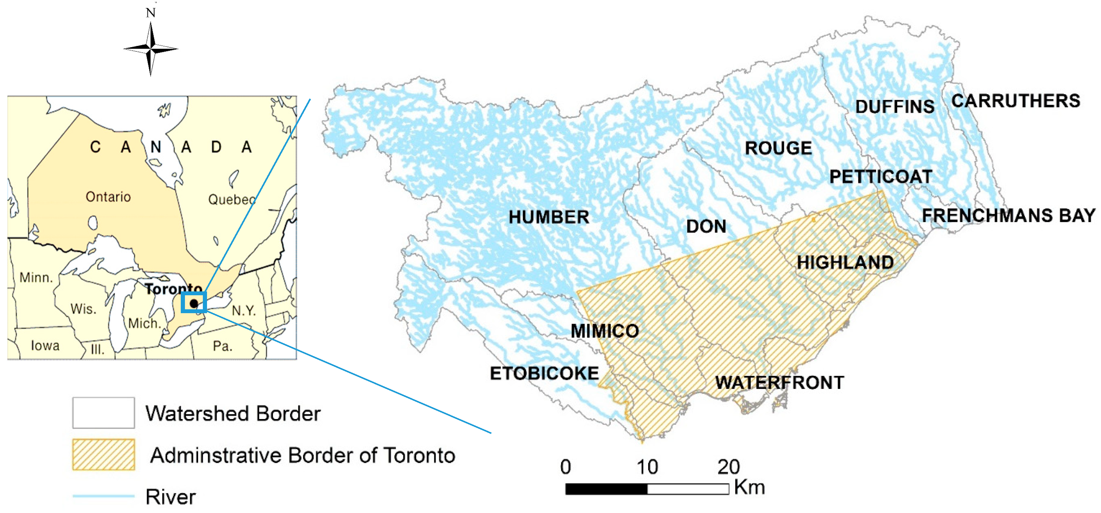
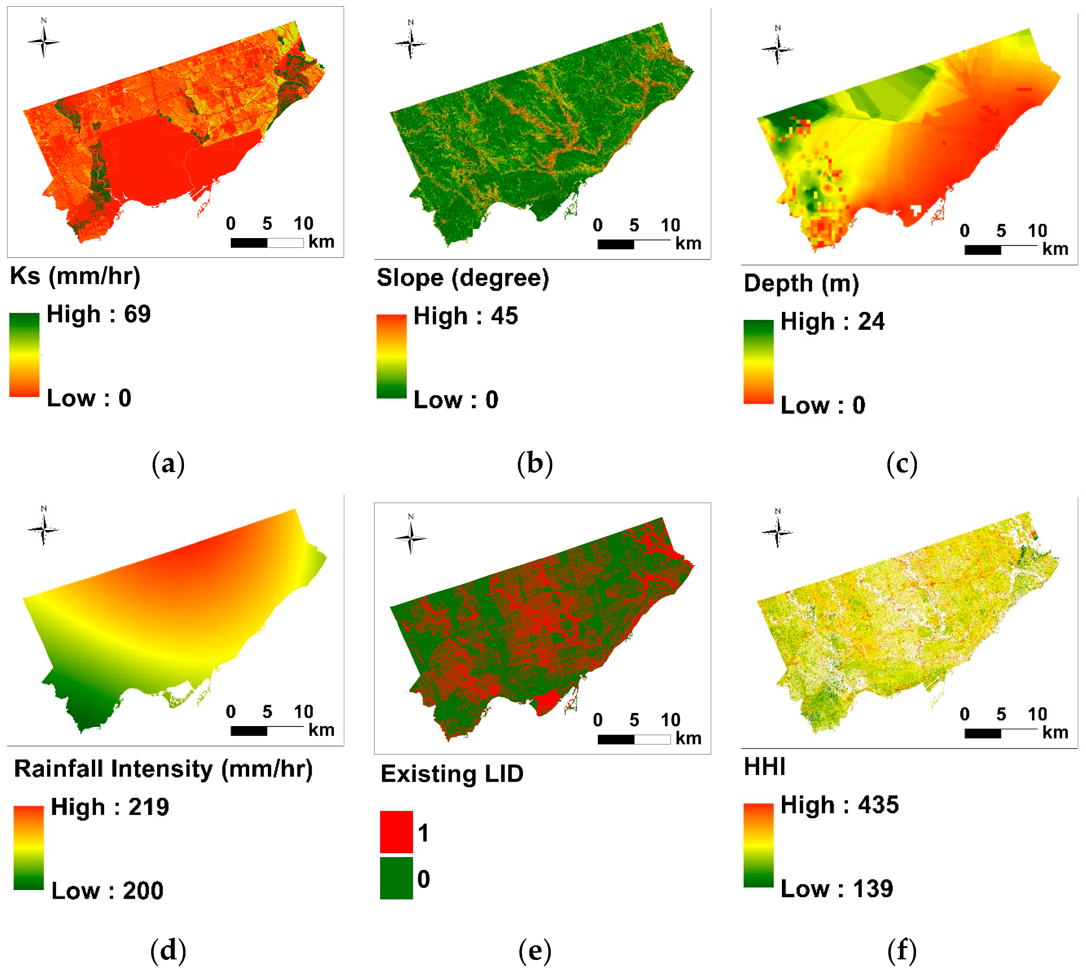
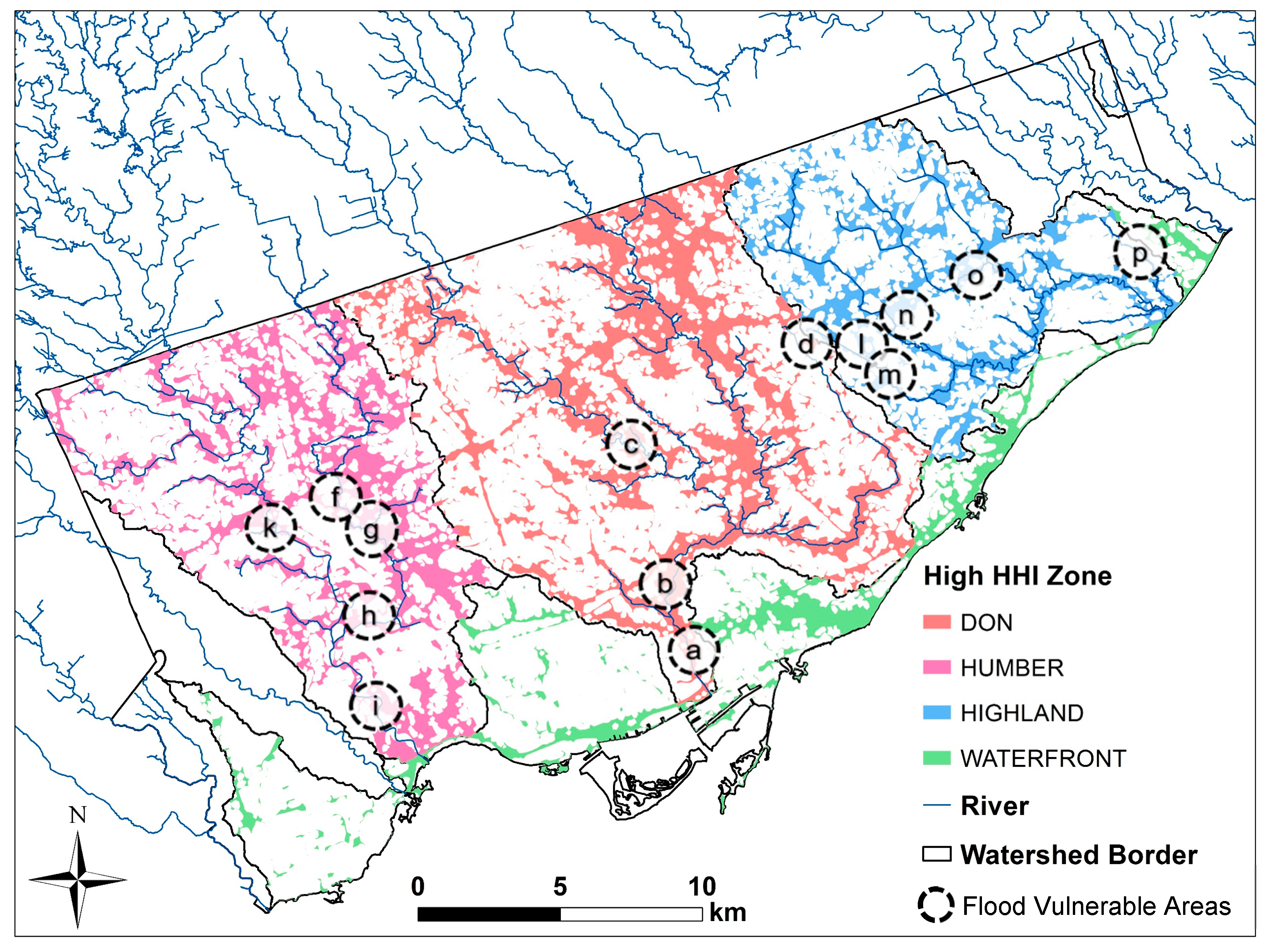
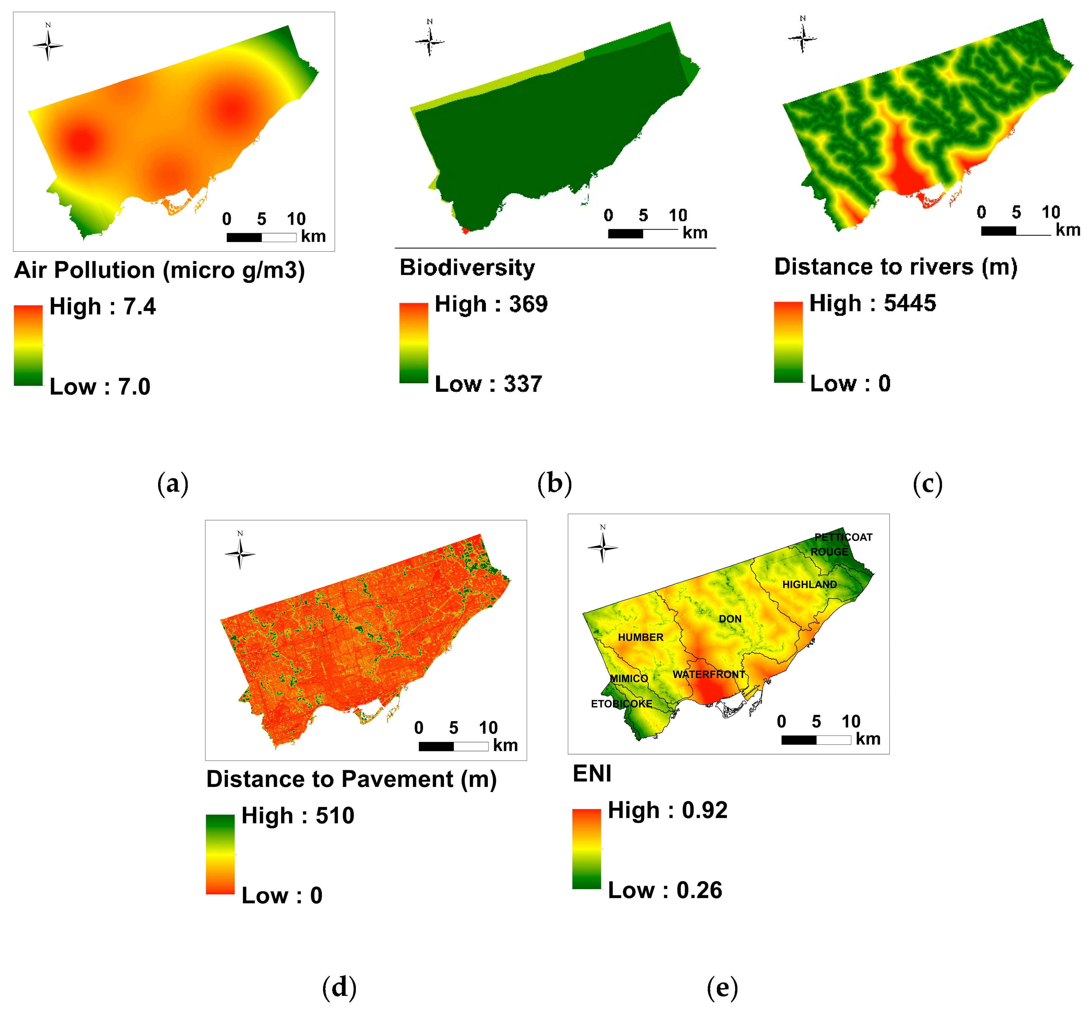
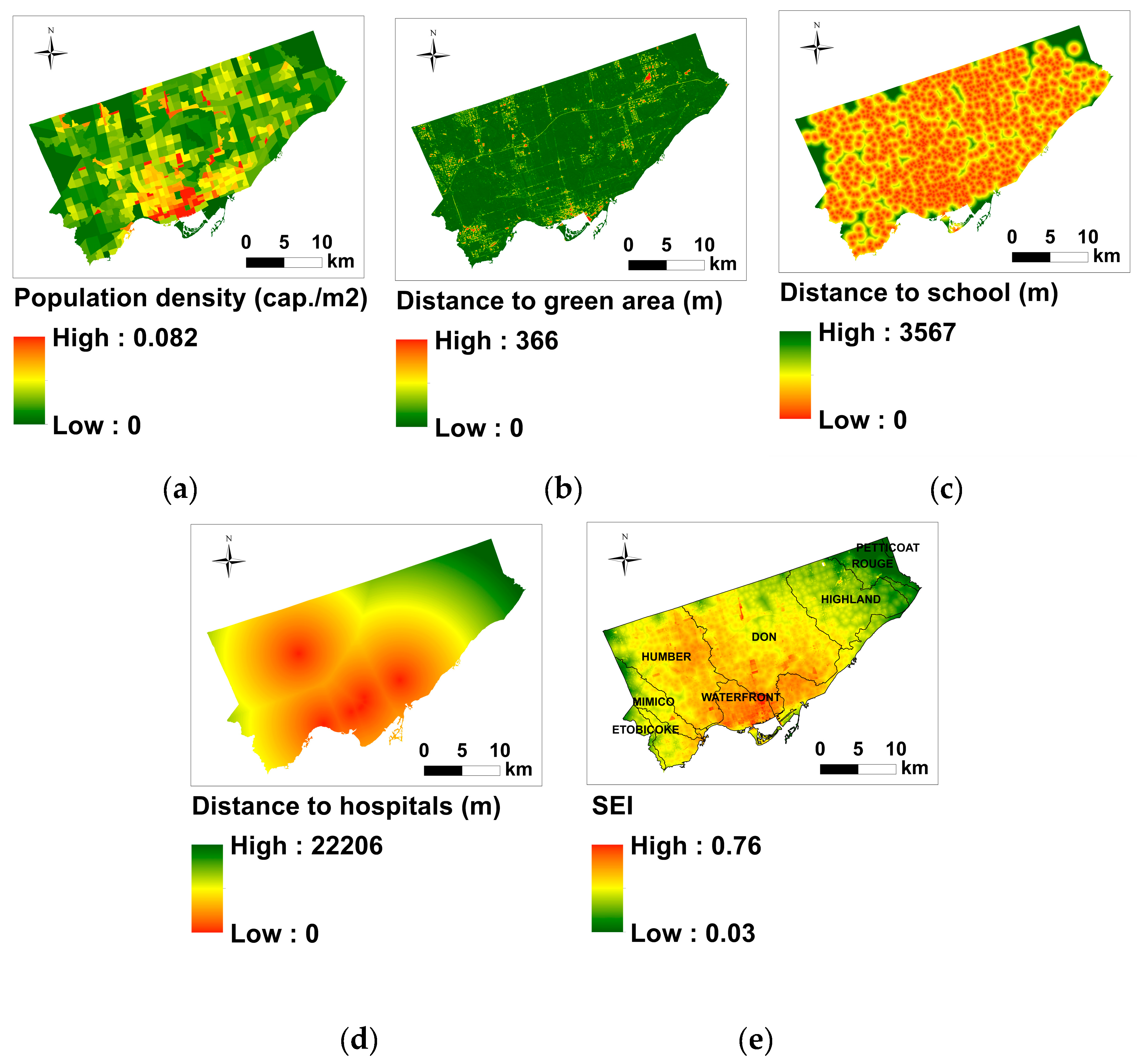
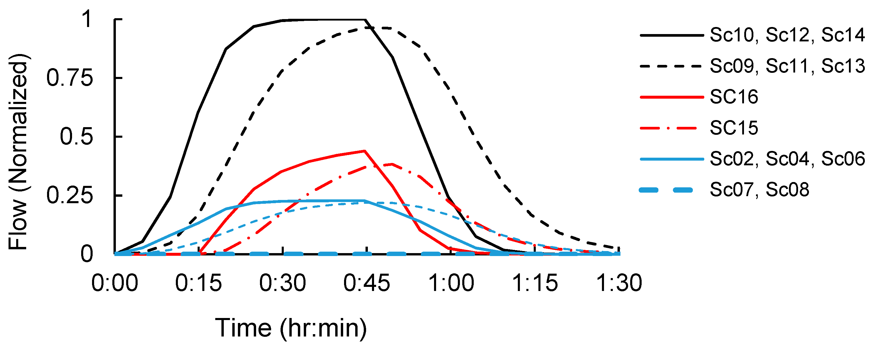
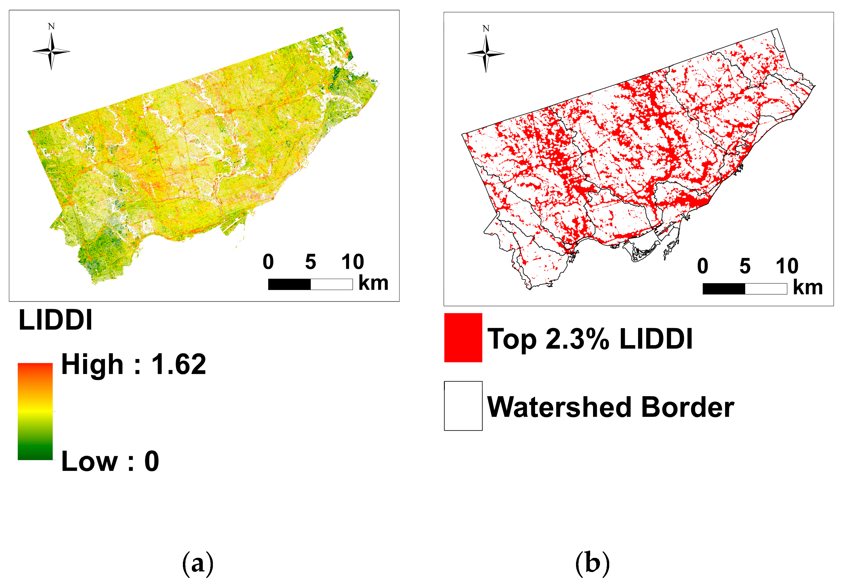
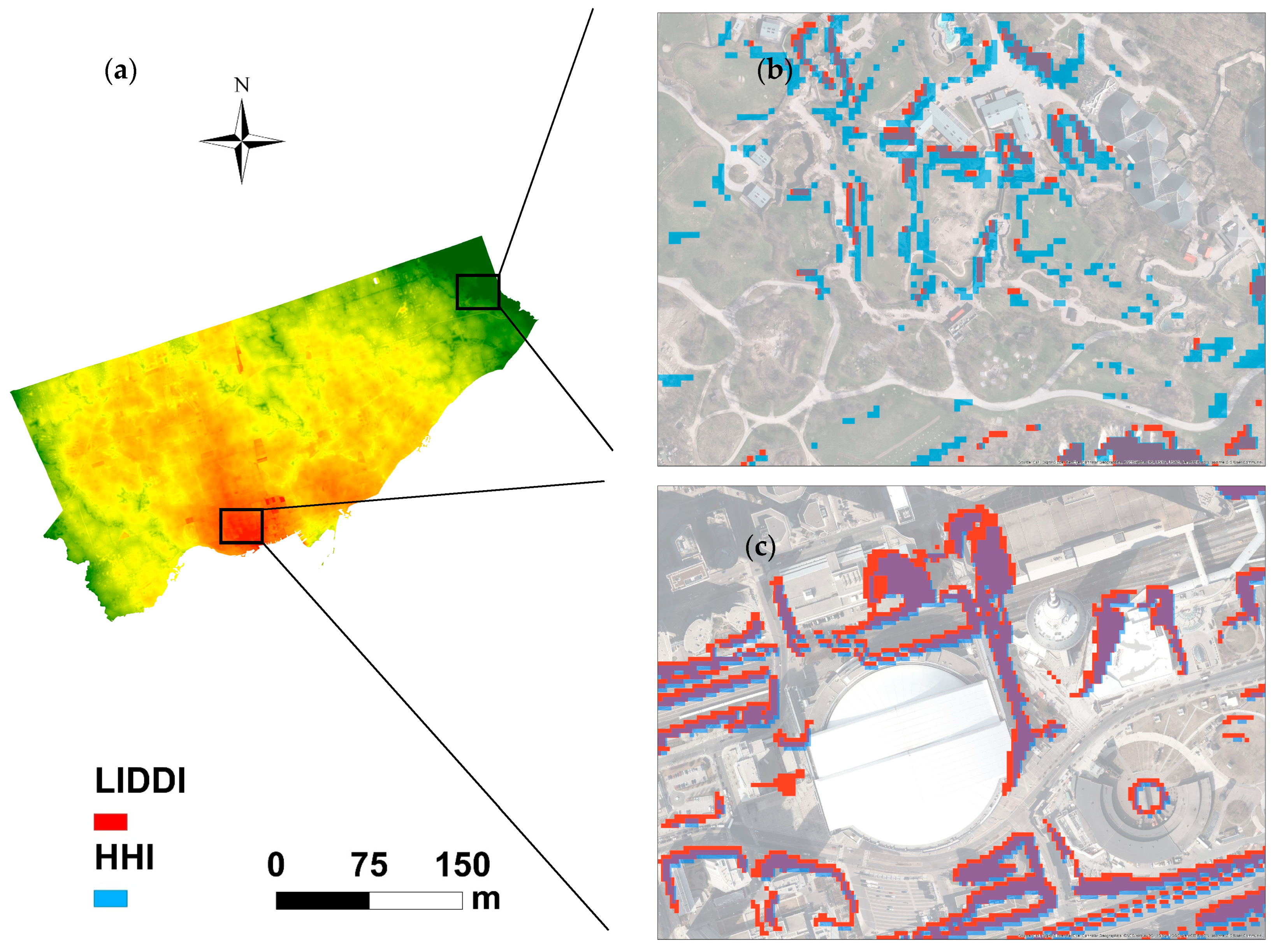
Table 1.
The raw data downloaded from publicly-available sources, including the structure/geometry of the data, and the source of the data.
Table 1.
The raw data downloaded from publicly-available sources, including the structure/geometry of the data, and the source of the data.
| ID | Data | Data Structure/Geometry | Data Source |
|---|---|---|---|
| 1 | Air pollution (PM2.5) | Vector/point | Ministry of Environment, Conservation and Parks |
| 2 | Bedrock layer | Vector/polygon | Ministry of Northern Development and Mines |
| 3 | Census tract boundaries 2016 | Vector/polygon | Statistics Canada |
| 4 | Demographics data-Census 2016 | Tabular data | Statistics Canada |
| 5 | Digital elevation model (DEM) | Raster/5 m × 5 m | Ontario Ministry of Natural Resources and Forestry-Provincial Mapping Unit |
| 6 | Ecozones of Ontario | Vector/polygon | Scholars Geoportal |
| 7 | Groundwater table | Vector/point | Groundwater Information Network (GIN) |
| 8 | Land cover | Raster/0.6 m × 0.6 m | City of Toronto |
| 9 | Toronto rivers | Vector/polyline | Toronto and Region Conservation Authority (TRCA) |
| 10 | Surficial geology and saturated hydraulic conductivity (Ks) | Vector/polygon | Government of Canada open data website |
| 11 | Toronto precipitation data | Vector/point | Government of Canada open data website |
| 12 | Educational institute | Vector/point | City of Toronto |
| 13 | Hospital | Vector/point | Google Earth |
Note: Missing data were ignored in the calculations.
Table 2.
The effect of the socioeconomic-environmental index (SEENI) on the hydrological-hydraulic index (HHI) in two sample cells.
Table 2.
The effect of the socioeconomic-environmental index (SEENI) on the hydrological-hydraulic index (HHI) in two sample cells.
| Cell # | HHI | SEENI | LIDDI | Rank |
|---|---|---|---|---|
| 1 | 0.9 | 1 | 1.8 | 1st |
| 2 | 0.9 | 0 | 0.9 | 2nd |
| 3 | 0 | 1 | 0 | 3rd |
Table 3.
Variable values considered for 16 scenarios.
| Variable | Low | High |
|---|---|---|
| R (mm/h) | 50 1 | 220 |
| D (mm) | 0 | 24000 2 |
| Ks (mm/h) | 0.3 | 117.8 |
| S (m/m) | 0.0001 | 0.15 3 |
1 Minimum R was not considered zero, allowing for generating a low amount of runoff. 2 The maximum D layer was selected according to maximum D of the study area. 3 The maximum S was considered to be 0.15 (=tan 9°), which is the greatest maximum proposed slope for all types of LID [57].
© 2019 by the authors. Licensee MDPI, Basel, Switzerland. This article is an open access article distributed under the terms and conditions of the Creative Commons Attribution (CC BY) license (http://creativecommons.org/licenses/by/4.0/).
Share and Cite
MDPI and ACS Style
Kaykhosravi, S.; Abogadil, K.; Khan, U.T.; Jadidi, M.A. The Low-Impact Development Demand Index: A New Approach to Identifying Locations for LID. Water 2019, 11, 2341. https://doi.org/10.3390/w11112341
AMA Style
Kaykhosravi S, Abogadil K, Khan UT, Jadidi MA. The Low-Impact Development Demand Index: A New Approach to Identifying Locations for LID. Water. 2019; 11(11):2341. https://doi.org/10.3390/w11112341
Chicago/Turabian StyleKaykhosravi, Sarah, Karen Abogadil, Usman T. Khan, and Mojgan A. Jadidi. 2019. "The Low-Impact Development Demand Index: A New Approach to Identifying Locations for LID" Water 11, no. 11: 2341. https://doi.org/10.3390/w11112341
Note that from the first issue of 2016, this journal uses article numbers instead of page numbers. See further details here.