Flood Inundation Mapping at Ungauged Basins Using Coupled Hydrometeorological–Hydraulic Modelling: The Catastrophic Case of the 2006 Flash Flood in Volos City, Greece

Abstract

Nowadays, as extreme weather increasingly threatens human health and economy, early warning system approaches are critical for timely preparedness and response. Towards the implementation of a multi-model forecasting system for flood hazards, this study presents a coupled application of three (3) models: The WRF-ARW weather model, the WRF-Hydro hydrological model, and the HEC-RAS 2D hydraulic model. A flash flood event that occurred on 9 October 2006 in Volos city, Greece, is used as a case study to assess the accuracy of the integrated modelling approach to simulate the flood hydrograph and flood extent in Xerias ungauged catchment. The hydrometeorological simulation results indicated a severe persistent storm over Pelion mountain at the northeast of Volos, as the main factor of the major flash flood and extensive impacts. Historical flood records retrieved by several conventional and non-conventional sources are used to validate the flooded area. Compared to the collected data and prior studies, the generated inundation map of Xerias river is found to realistically capture highly impacted areas which experienced infrastructure damage and human rescues from inundated roads and buildings. Results from our analyses show that the proposed physically-based modelling approach can give reliable inputs into flood risk management.

1. Introduction

Last century, extreme hydrometeorological hazards were considered to be one of the most critical natural hazards that caused substantial damages to natural and man-made environments. Based on the EM-DAT database, during the period 1900–2019, Europe experienced 1121 extreme hydrometeorological events that caused 13,019 deaths, affected about 25,657,172 people, and cost $250 billion [1]. At a global scale, floods are one of the most devastating hydrometeorological disasters, responsible for a high percentage of mortality and other social, economic, and environmental damages, including infrastructure damages, property loss, displacement, crop destruction, sediment and nutrient transport, habitat loss, etc. [2]. A number of studies have indicated that the intensity and the number of extreme flood events have increased during the last decades. There is, also, a strong correlation between this trend and the increase of human activities, such as changes in land-use patterns and expansion of economic activities [3].

Sustainable flood risk management strategies and flood mitigation measurements have received much attention over the last two decades due to the increasing intensity, frequency, and magnitude of the severe flood events [2,3]. The European Union adopted the Directive 2007/60/EC for the assessment and management of flood risks. A key objective of this Directive is the formation of a generic framework for flood hazard and risk modelling and mapping to mitigate the adverse consequences of floods to the environment, human health, general economic activity, and sites of cultural heritage value [4]. The implementation of the Directive 2007/60/EC is an ongoing process, and all EU member states are obligated to revise the flood management plans every six (6) years. European countries are invited to exploit the most recent hydrometeorological advancements and to account for particular sensitivities and capacities of their population to assess flood risk at the local, regional, or national levels. In the disaster management chain, results from flood inundation modelling and mapping feed the establishment of flood risk assessments, in which physical processes should be examined in line with local vulnerabilities and societal dynamics to inform the development of floodplain management and mitigation strategies. Therefore, the selection of appropriate and effective tools for flood inundation modelling and mapping is a critical process for the implementation of the Directive 2007/60/EC [5].

The implementation of flood risk management and mapping demand some major flood characteristics, such as the flood water depth, the flood extent and duration, the flood flow velocity, and the resilience of structures’ stability to floods. Therefore, river flood modelling, mapping, and risk management are usually defined with the use of several one-dimensional (1D) and/or coupled (1D/2D) and/or two-dimensional (2D) hydraulic–hydrodynamic models (e.g., [2,6,7,8]). Recent studies feature the capabilities of these models for the precise estimation of several flood characteristics and for advanced flood inundation modelling and mapping (e.g., [9,10,11,12]). Furthermore, flood characteristics are affected by the surface water runoff and, subsequently, by the preceded precipitation. In-situ and remote sensing observational systems can provide accurate quantitative precipitation estimates, which serve as input to hydrological models to simulate runoff routing [13]. The hydrological modelling outputs can be inserted, then, in hydraulic–hydrodynamic models for rigorous flood inundation modelling and mapping. Nevertheless, spatiotemporal limitation of the observational systems usually necessitates numerical weather prediction models to provide quantitative precipitation forecasts. In this context, coupled hydrometeorological modelling systems can be exploited to reduce uncertainties associated with observations while representing atmospheric, soil, and hydrological processes in a physically-based way.

In recent years, there is an increasing trend of using one-way or two-way coupled hydrometeorological modelling systems. Typical studies use the Weather Research and Forecasting model (WRF) [14,15] and hydrological models such the WRF-Hydro model [16]. Several studies that apply hydrometeorological simulations for either flood forecasting or long-term predictions indicate the importance of integrated atmospheric, soil, and hydrological modelling tools [13,17,18,19]. Sanz-Ramos et al. [20] yield encouraging results using coupled meteorological and hydrological modelling to force a hydraulic model aiming at flood forecasting over a topographically complex Spanish region. It appears that coupled hydrometeorological modelling systems are very useful, especially for catchments characterised by complex terrain.

Over the last decades, there has been an increasing number of studies on flood events for which a sufficient amount of data for verification is available (e.g., stage and discharge relationships, discharge data, accurate rainfall data, satellite flood extent, flood peak watermarks) [9,21,22,23,24]. However, in ungauged or poorly gauged catchments, flood-related data (i.e., hydrometeorological data and/or flood inundation data such as flooded area and measured water depth-watermarks) are inadequate, both quantitatively and qualitatively. In such cases, the implementation of flood inundation modelling is limited. This is particularly true for urban and suburban areas, where the hydraulic–hydrodynamic configuration is much more demanding and complex (e.g., due to the existence of bridges, flood retention works, buildings, roads) [6,7,10,25,26,27]. Most of these studies use Synthetic Unit Hydrographs (SIUH) methods to determine the synthetic flood hydrographs for a defined return period. The analysis of extreme case study events for suburban–urban flooding in ungauged catchments is subject to limited observations and often requires non-trivial post-event investigations [3,28]. Therefore, although there are many studies in the literature, only a few studies deal with real-world cases that can be effectively used for the calibration and/or validation and assessment of the numerical models [7].

To fill this gap, this study aims to build a combined weather, hydrological, and hydraulic–hydrodynamic modelling approach for flood inundation modelling and mapping at ungauged watersheds. The presented methodological approach proposes the combination of the WRF-ARW weather model [14], the WRF-Hydro hydrological model [16], and the HEC-RAS 2D hydraulic–hydrodynamic model [29]. The proposed methodology was applied first for fluvial flood modelling and mapping at Xerias watershed to simulate the extreme flash flood event that took place on 9 October 2006, in the suburban and urban area of Volos city, Thessaly region, Greece. Based on prior analysis, the study event caused severe flooding with an estimated return period equal to 100 years [10,30]. The flash flood of 9 October 2006 was an extreme event, and it was selected for its unique devastating socio-economic effect on the city of Volos and the surrounding area. To our knowledge, this study is the first coupled hydrometeorological–hydraulic analysis of Xerias watershed case study (Magnesia, Greece), which is challenged by the lack of flood-related data and measurements. In this objective, the authors’ retrieved historical flood records from several sources to be used for the validation of the floodplain. Results of this research are also compared with flood maps generated using flood hydrographs developed in previous studies [5,6,10].

2. Materials and Methods

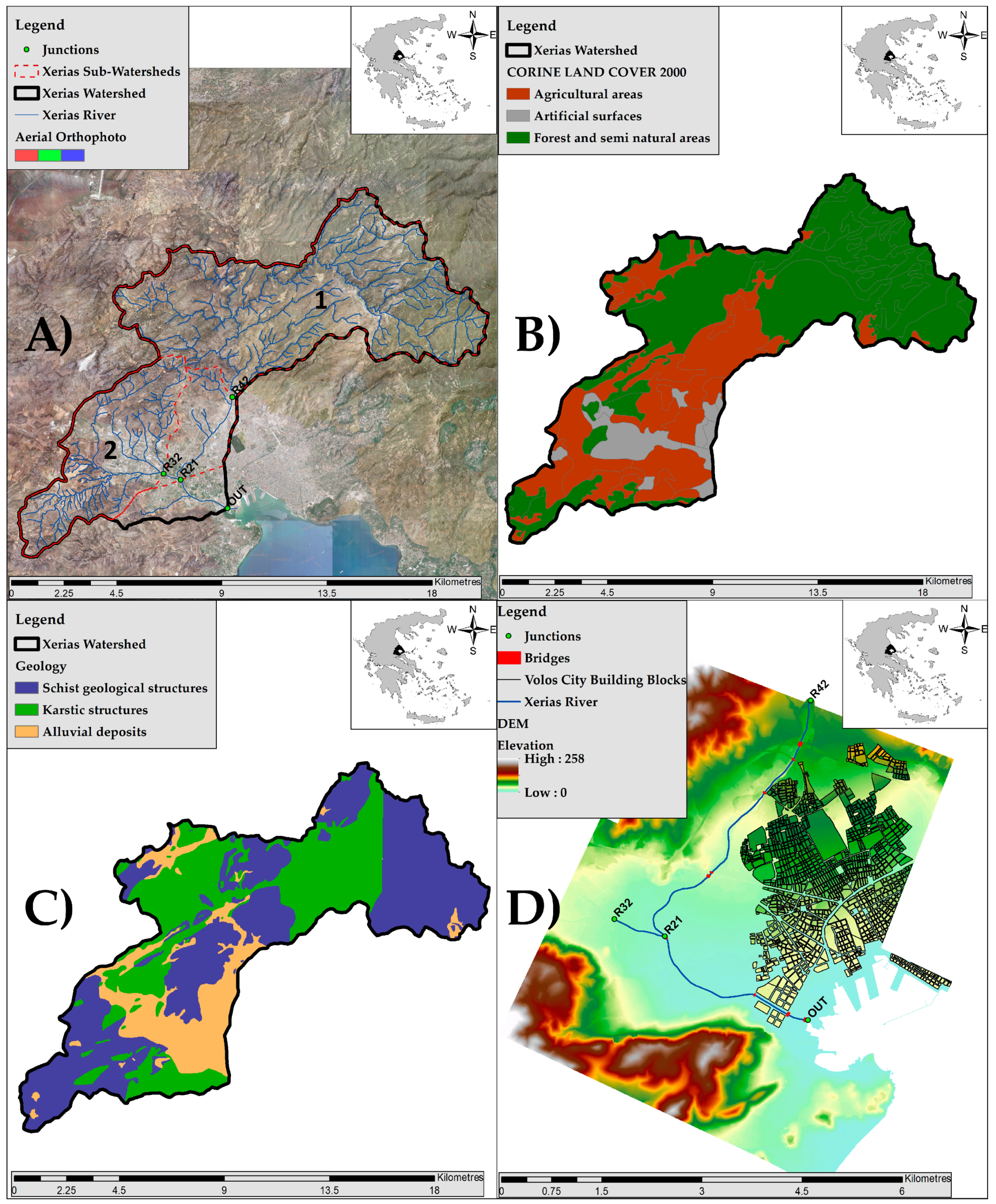
A combined weather, hydrological, and hydraulic–hydrodynamic modelling approach was applied for flood inundation modelling and mapping at Xerias ungauged watershed. The hydrometeorological approach was based on the combination of the WRF-ARW weather model and the WRF-Hydro hydrological model. Finally, the hydrographs derived from the hydrological model were used as input hydrographs in the 2D HEC-RAS hydraulic–hydrodynamic model for flood inundation modelling and mapping. For comparison purposes, three different input hydrographs were used for the river flood modelling and mapping. Conventional and non-conventional flood data and impact records of the extreme flash-flood event that occurred on 9 October 2006 were used for the validation of the simulated flood extent in Volos city area. The flood extent validation procedure was based on the estimation of the percentage of the validation data observed within the simulated flood extent. This validation approach was chosen due to the severe lack of flood-related data, such as gauged measurements, measured water depth, and other hydraulic characteristics. However, in order to implement a rough estimation of the model performance in terms of water depth, relevant photos and press documentary were used to assess the observed water depths in specific locations. This approach allowed for a rough comparison between the observed and simulated water depths.

2.1. Study Area

Volos city is located in the south-eastern part of Thessaly region, Magnesia prefecture, Greece, and it is the sixth-largest city of Greece, with respect to human population. Volos city has a population of approximately 145,000 people based on 2011 population census [31]. Xerias watershed lies between latitude 39°20′0′′ to 39°28′41′′ N and longitude 22°49′22′′ to 23°03′15′′ E (Figure 1A). Moreover, the selected watershed has an area of approximately 120 km²; elevation ranges from 0 to 1600 m, and the average and median elevation of the watershed is 458 m and 320 m, respectively. The main sub-watersheds of Xerias, are the: (1) Upper Xerias sub-watershed (outlet R42), (2) Seskouliotis and Kakaviotis sub-watershed (outlet R32) (Figure 1A). Based on decadal (February 2007–July 2017) data retrieved from the Meteorological Station of Volos (National Observatory of Athens (NOA) network), the average annual temperature is 17.8 °C and the mean monthly temperature ranges from 8.4 to 28.4 °C. The climate is typical Mediterranean, with hot and dry summers, and with temperatures sometimes reaching up to 40 °C. The mean annual precipitation ranges from 400 to 770 mm with the autumn, winter, and spring being the wet seasons. The determination of the land cover was based on CORINE LAND COVER 2000 data (CLC2000). The largest part of the watershed is covered by forest and semi-natural areas (57%), followed by agricultural areas (36%) and artificial surfaces (7%) (Figure 1B). The geological map of the study area has been derived from the Institute of Geology and Mineral Exploration (IGME) (scale 1:50,000). The majority of the study watershed is covered by Schist geological structures (49%), followed by karstic structures (35%) and alluvial deposits (16%) (Figure 1C). As can be seen in Figure 1D, Xerias stream flows through the city of Volos into the sea. Quite often, the city of Volos experiences extended flash flood events due to intense storms, resulting in significant damages of several public infrastructures (e.g., roads, railways), buildings, local infrastructures, and agricultural areas (e.g., 2003, 2006, 2009, 2012) [32,33,34,35].

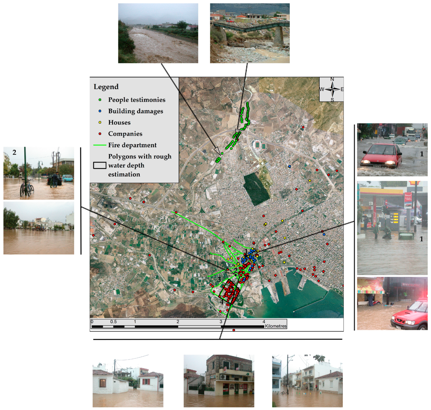
2.2. Flood Data Collection

On 9 October 2006, the city of Volos experienced the devastating effects of heavy rainfall that lasted approximately 12 h and caused extended fluvial and pluvial flooding. Fortunately, no human lives were lost, but Volos city underwent severe economic losses and damages on the transportation networks, buildings, and agricultural areas. The rainfall activity of the extreme flash flood event is presented in the following sub-section. According to prior analysis, the return period of the study event is estimated at about 100 years [10,30].

Unfortunately, no conventional hydraulic data (i.e., data from gauged stations such as discharge or water depth) were available for the study event. Therefore, the effort of the flood data collection targeted every possible source of flood-related information. Some crucial comments about the flood data collection are: (1) The total amount of data was large, but their quality and their usability was limited, (2) the official flood-related data were scattered to several governmental authorities, (3) the original data were in printed format and/or handwritten forms, (4) the human factor might bias several steps of the process (e.g., evaluation of flood extent testimonies), and (5) the bureaucracy sometimes delayed the entire procedure. Creating a flood dataset for the 9 October 2006 flood event was a time-consuming process, and the several steps from collection (contacts and gathering) to processing (digitisation and categorisation) and evaluation (assessment of data validity/quality) lasted about six months. Non-conventional flood data collected for hydraulic modelling set up and calibration and/or validation of the flood event are categorised to [7]: (1) Damage estimation reports, (2) photos, (3) videos, (4) local mass-media reports, and (5) interviews with eyewitnesses or judicial reports. Unfortunately, no post-event reports on surveying flood watermarks were documented.

2.2.1. Damage Estimation Reports

The damage reports were collected by several authorities, such as the Administration of Technical Works (Decentralized Administration of Thessaly Region), the Welfare Department of Volos Municipality, and the Fire Department of Volos city. All these reports were provided in printed documents and/or handwriting forms, except for some of the Administration of Technical Works data that were digitised data in Excel© format. All collected data underwent quality checking. Administration of Technical Works provided the addresses and data related to economic losses from all companies (see companies depicted with red points in Figure 2) and the addresses of buildings (see building damages depicted with blue points in Figure 2) that were affected by the flooding. Only three to four records from the Administration of Technical Works data included photos of the aftermath of the flood event (i.e., damaged products and machinery). The Fire Department of Volos city presented a document with the flooded streets, with a rough estimation of the water depth considered as homogeneous in all of the flooded streets (i.e., water depth = 2 m in all streets) and therefore, it could not be used for further analysis. The Welfare Department of Volos Municipality provided the addresses of houses that were refunded for electrical appliance damages (see houses shown with yellow points in Figure 2). All of the aforementioned information was used in combination with Google Maps to identify (when that was possible) the location of each element-record. Later, all records were digitised in a GIS environment (Figure 2). Based on the characteristics of the damage estimation records, the use of this dataset is restricted to the delineation and the visualisation of the spatial distribution of the flood extent under study.

2.2.2. Photos and Videos

The authors did not find any videos that could provide valuable information on the post-flood survey. On the other hand, several photos that were captured during the flood event were provided by the local amateur meteorologists Mr. Solonas Tsakiris and Mr. Stavros Dafis, and the local newspapers “Thessaly” and “Taxydromos”. It was possible, with the use of Google Street View (Google Maps), to obtain the location of several places based on authors’ personal knowledge of the study area. Therefore, in this analysis, we examined the possibility to locate spatially the photos provided by the several sources. Most of the photos were accessible through the local newspaper “Thessaly”, which was the main provider of photographic documentary, and they were assigned mainly to four locations (see photograph locations in Figure 2). Additional photos referring to the upper part of Xerias stream were gathered from the personal collections of Mr. Solonas Tsakiris and Mr. Stavros Dafis. In this analysis, the majority of the collected photos were used for the validation of the flood extent in specific locations. Supplementary image analysis was conducted using some of the collected photographs to produce quantitative flood data, such as observed water depths. Specifically, two (2) photographs from location n.1 and one (1) from location n.2 were selected as relevant for a rough estimation of the water depth (Figure 2). The selected photographs offer good visibility of the height of floodwater, and they illustrate other elements that could be used as reference points for comparison with the assumed water depth. These photographs cover a specific area and the locations do not have significant elevation differences. Therefore, two (2) polygons that cover an area around the validation point extracted from the photographs were created and assigned with a single estimate of the observed water depth (Figure 2, polygons and photos n.1, n.2). Moreover, the use of these polygons provided a more reliable way to compare the observed water depth with the median simulated values. It is noteworthy to mention that we should not relate the obtained water depth observations with the maximum water levels reached during the study event. Given that the capture time of the photographs was several hours after the peak flow, it would be reasonable to correlate the observed water depths with the levels at which the floodwater remained for the longest time, rather than the largest water levels observed at the time of the peak.

2.2.3. Local Mass-Media Reports

Several articles from the local newspapers were examined to provide supplementary information about the flood event. Unfortunately, the majority of the quantitative information that could be retrieved from articles and news reports had been already obtained from other data collected for the study flood event. However, the local press provided empirical evidence that confirmed the severity of the event in given locations and enhanced our understanding of its impact on the society of Volos. Specific descriptions provided by the local mass media reports were used to draw two (2) polygons in which a single water depth estimate could be assigned (Figure 2, polygons n.3, n.4).

2.2.4. Interviews with Eyewitnesses and/or Judicial Reports.

The authors did not find any Judicial reports regarding the study flood event. However, several interviews were implemented in the upper part of Xerias stream, where complex hydraulic conditions existed due to the presence of three successive bridges, including the railway bridge that collapsed during the event (Figure 2). The interviews were focused on the upper part of the study area due to: (1) The absence of other flood-related data sources at that area, (2) the severe damages on the railway network during the event, and (3) the complexity of the river topography [10]. Unfortunately, none of the interviewees could provide accurate estimates for the flood water depth values. Thus, the outcome from the interviews contributed mainly to the delineation of the flood extent. It should be noted that some of the testimonies were classified as unreliable because the interviewee gave misleading information for the flood extent.

To summarise, the majority of the collected flood data is distributed in the lower part of Xerias stream and mainly inside the area of Neapoli and Pedion Areos districts southwest of Volos city (Figure 2). Neapoli and Pedion Areos areas experienced a great number of damages in buildings and properties. These regions are characterised by high commercial activity with commercial buildings accounting for up to 75% of the total buildings (residencies and companies). The commercial use of the buildings, in conjunction with the existence of old structures in which companies and stores are located, makes the area particularly vulnerable in terms of economic damages by a flood event. Refunds from the Greek government to Neapoli and Pedion Areos, and especially to company and stores owners, were estimated to be approximately 3.96 million euros. Eighty percent (80%) of the companies that demanded governmental support in the aftermath of the flooding were located in Pedion Areos area that extends north of Neapoli area. The spatially distributed flood data processed by the authors were examined based on experts’ judgment, the local mass-media reports, and the collected photographs to generate the flood extent validation dataset. The digitised data can be used for the validation of the flood extent. However, reliable references to the observed water depths are rare. The scattered records that appear in the right part of Figure 2 relate to pluvial flooding incidents and were omitted from this analysis. However, these scattered records prove the severity of the extreme hydrometeorological event that caused fluvial and pluvial flood in Volos city. The fire department records were transformed from polyline features to point features based on the Digital Elevation Model’s (DEM’s) spatial resolution in order to use them in a manageable format for the validation procedure. Finally, the records from the people testimonies, building damages, houses, and companies consisted of 353 point features, while the fire department records consisted of 3903 points, yielding a total of 4256 flood extent validation points (named validation data hereafter).

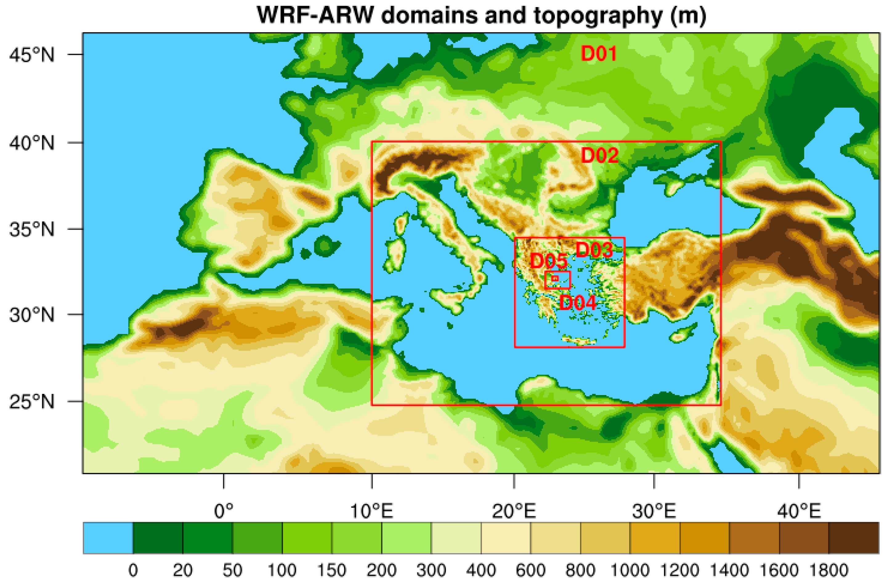
2.3. Μeteorological Analysis Methods and Weather Model Setup

Firstly, the synoptic-scale meteorological conditions before and during the flash flood event were analysed. The synoptic meteorological conditions often determine the formation and evolution of extreme weather events causing floods and extensive damages (e.g., [36,37,38]). The synoptic meteorological analysis was performed using the Global Forecasting System (GFS) operational analyses of the National Centers for Environmental Prediction (NCEP) with a horizontal resolution of 1.0 × 1.0°. This analysis was based on the combined use of mean sea level (MSL) pressure and upper-air parameters such as temperature and geopotential height. In this way, the barometric systems at the surface and the upper air systems, such as troughs and ridges, can be detected and analysed. This supports the investigation of the contribution of synoptic conditions on the evolution of the severe storm causing the flood of 9 October 2006.

The WRF-ARW version 4.0 weather model [14,15] was used for the investigation of dynamical and thermodynamic factors leading to the severe weather conditions during the hydrometeorological event, as well as for the construction of a meteorological forcing dataset to be used in the hydrological simulation. The WRF-ARW model was selected because it offers advanced capabilities in high-resolution simulation of severe weather phenomena [39,40,41,42,43]. WRF-ARW was configured to perform a 72-h simulation from 8 October at 00:00 UTC to 11 October at 00:00 UTC to resolve the meteorological processes during the lifecycle of the severe storm which occurred during the period from 06:00 to 18:00 UTC on 9 October with total measured precipitation in Volos city of about 232 mm [44]. Even though the storm occurred on 9 October, the weather simulation lasted until 11 October at 00:00 UTC to generate meteorological forcing data even after the occurrence of the flash flooding. This extension in the simulation period facilitated the simulation of hydrological processes which had a delayed response compared to the meteorological event (e.g., [45]).

WRF-ARW was set up using multiple nests on five (5) domains with horizontal resolutions of 36 × 36 km, 12 × 12 km, 4 × 4 km, 1 × 1 km, and 0.25 × 0.25 km (Figure 3). Time steps of 180, 60, 20, 5, and 1 s were used for the five (5) domains, respectively. The initial conditions for 8 October at 00:00 UTC were based on the GFS operational analyses with a horizontal resolution of 1.0 × 1.0°. The boundary conditions were also based on the GFS operational analyses with a time step of 6 h. The initial sea surface temperature (SST) field for 8 October was based on the real-time global (RTG) SST analyses with a horizontal resolution of 0.083 × 0.083° produced by the NCEP. The initial SST was preserved constant for the 72-h simulation period because a testing simulation which had been performed applying RTG SST update every 24 h was below expectations regarding the 232 mm of precipitation measured in Volos city during the period from 06:00 to 18:00 UTC on 9 October 2006 [44]. The Global Multi-resolution Terrain Elevation Data (GMTED 2010 30-arc-sec USGS) [46], the vegetation data MODIS FPAR [47], and the 21-class IGBP MODIS [48] land-use data were used as static input data in the WRF-ARW model procedures.

As far as the modelling schemes of meteorological mechanisms are concerned, the Yonsei University scheme (YSU) [49] and the revised Monin-Obukhov scheme [50] were used to resolve the Planetary Boundary Layer (PBL) and the surface layer processes, respectively. The ground processes were parameterised using the unified land surface model [51] (Unified NOAH). In order to represent the long-wave and short-wave radiation processes, the RRTMG scheme [52] was used. In order to simulate the cloud microphysical processes, the Thompson scheme [53] was used. For the simulation of the convective processes, the Grell–Freitas ensemble scheme [54] was used in the first three domains (36 × 36 km, 12 × 12 km, and 4 × 4 km), while explicit solution was selected for the fourth (1 × 1 km) and the fifth (0.25 × 0.25 km) domains.

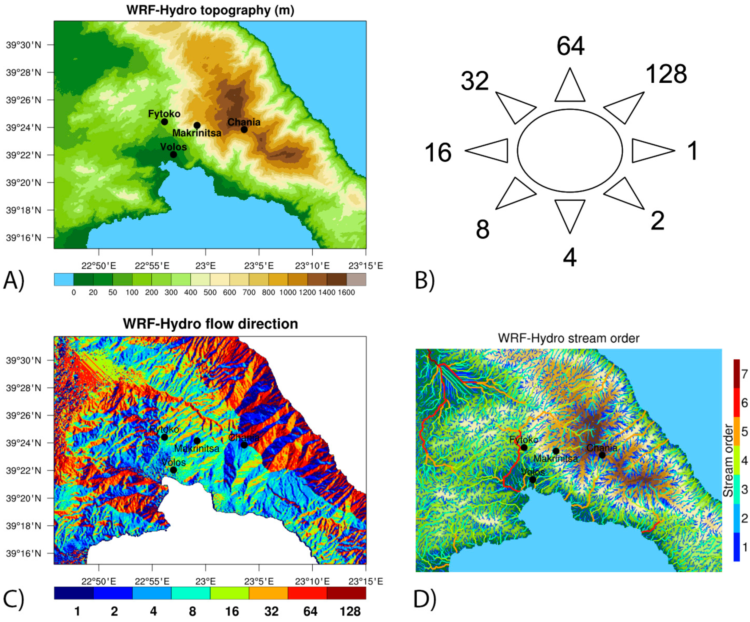
2.4. Hydrological Model Setup

The aim of this study was to simulate not only the meteorological conditions, but also the hydrological processes of the flash flood event. For this reason, the results of the weather model on the fifth domain (0.25 × 0.25 km) were used to force the WRF-Hydro version 5.0 hydrological model with a forcing time step of 1 h. The meteorological forcing fields are presented in

Table 1. The seven meteorological forcing fields [16].

Meteorological Forcing Fields	Units
Incoming shortwave radiation (SR)	(W m−2)
Incoming longwave radiation (LR)	(W m−2)
Air specific humidity at 2 m (Q2)	(kg kg−1)
Air temperature at 2 m (T2)	(K)
Atmospheric pressure at surface (PSFC)	(Pa)
Near surface wind at 10 m in the u- and v-components (U10, V10)	(m s−1)
Liquid water precipitation rate (PREC)	(mm s−1)

. The WRF-Hydro model was selected because it is one of the most burgeoning hydrological models with encouraging results [13,17,19,55]. Furthermore, it is worthwhile noting that WRF-Hydro is employed as a framework for bridging atmospheric and hydrological modelling at the National Water Center of the United States [56]. The methodology followed to set up WRF-Hydro for this study was similar to the one applied in a recent paper [13] for the simulation of a flash flood event in Mandra, western Attica, Greece. Thus, in this study, the model was set up on the extent of the fifth domain (0.25 × 0.25 km) of the weather model, including the drainage basin of Xerias stream, which is depicted on the five-times finer horizontal resolution of 50 × 50 m (Figure 4A).

As far as the topographic data of hydrological modelling are concerned, the Shuttle Radar Topographic Mission (SRTM) Digital Elevation Model (DEM) [57] data of National Aeronautics and Space Administration (NASA) on the native horizontal resolution of 90 × 90 m were used. In particular, the void-filled version [58] of this dataset distributed by the Hydrological Data and Maps Based on Shuttle Elevation Derivatives at Multiple Scales (HydroSHEDS; https://hydrosheds.cr.usgs.gov/index.php) was selected to be employed. The WRF-Hydro pre-processing tool [16] was applied to regrid DEM on the 50 × 50 m horizontal grid using bilinear interpolation. Moreover, static input data such as topography (Figure 4A), flow direction (see Figure 4B,C), channel grid and stream order (Figure 4D), which were appropriate for the hydrological modelling, were constructed using this tool (for technical information, see [16]). Furthermore, the pre-processing stage [14] of the WRF-ARW model was used to initialise land surface parameters such as soil temperature and soil moisture, as well as to construct soil type, land use, and vegetation fields used in the land surface model (LSM) NOAH [16] of the WRF-Hydro model. The land surface data on 30-arc-sec native horizontal resolution was regridded to the grid of the fifth domain of the WRF-ARW model on horizontal resolution of 0.25 × 0.25 km, and, afterwards, to the grid of WRF-Hydro domain on horizontal resolution of 50 × 50 m. For the two regridding procedures, the bilinear interpolation method was employed.

2.5. Hydraulic Model Setup

The HEC-RAS model was used for the hydraulic routing simulation of flood hydrograph through the Xerias stream network. The HEC-RAS model is a well-known hydraulic–hydrodynamic model developed by the Hydrologic Engineering Center (HEC) of United States Army Corps of Engineers, and used for river flood modelling and floodplain management (e.g., [6,59]). The efficiency of the two-dimensional (2D) HEC-RAS model has been examined using the United Kingdom’s (UK) Joint Defra (Department for Environmental Food and Rural Affairs) Environment Agency benchmark tests. Results from this benchmark analysis showed that the two-dimensional (2D) HEC-RAS model could produce comparable results to the two-dimensional models reported by the research report of the United Kingdom Environmental Agency [60,61]. Therefore, in this analysis, the two-dimensional (2D) HEC-RAS model was used for flood inundation modelling and mapping. It should be mentioned that the hydraulic model setup was prepared in accordance with the configuration proposed in a recent paper [5].

The importance of DEM’s accuracy has been highlighted by several authors, especially in two-dimensional hydraulic–hydrodynamic modelling applications [6,62,63]. Flood inundation modelling and mapping at urban and suburban areas demands sufficient DEM resolution, and the represented topography should be chronologically close to the study flood event [7,64]. In order to meet these requirements, a DEM with horizontal resolution of 5 × 5 m generated from aerial images collected from 2007–2009 and provided by the National Cadastre and Mapping Agency S.A. (NCMA) was used in this study.

Another critical parameter in hydraulic–hydrodynamic modelling applications is the roughness coefficient. Therefore, an essential process in river flood modelling and mapping is the methodological approach followed for the roughness coefficient estimation [65,66]. A standard approach followed in river flood modelling was the use of typical roughness coefficient tables in combination to CORINE land cover data [5,67]. The values of the roughness coefficient proposed in a recent paper [5] were used in this study (

Table 2. Study area of Manning’s roughness coefficient based on CORINE land cover data [5].

LABEL3	Manning’s n
1.1.1 Continuous urban fabric	0.013
1.1.2 Discontinuous urban fabric
1.2.1 Industrial or commercial units	0.013
1.2.3 Port areas
1.3.1 Mineral extraction sites	0.013
1.3.3 Construction sites
2.2.2 Fruit trees and berry plantations	0.08
2.2.3 Olive groves
2.4.2 Complex cultivation patterns	0.04
2.4.3 Land principally occupied by agriculture, with significant areas of natural vegetation	0.05
3.2.1 Natural grasslands	0.04
3.2.3 Sclerophyllous vegetation	0.05

).

Another factor that affects flood inundation modelling, especially at urban and suburban areas, as well as when using a two-dimensional hydraulic model, is the accurate representation of the technical works (e.g., flood protection works, culverts, bridges, weirs, etc.) within the hydraulic modelling domain. In this study, all hydraulic structures were detected using aerial photographs, field observations, and data from different authorities. Topographical surveys were conducted to record the characteristics of significant hydraulic structures [5]. All data related to hydraulic structures were used to modify/correct the DEM and, within the hydraulic modelling geometry configuration, to depict structures such as bridges, culverts, etc. The final hydraulic modelling domain, within the two-dimensional (2D) HEC-RAS model, includes nine (9) bridges in the main channel (Figure 1D), represented as combinations of culverts and weirs.

Urban flood inundation modelling and mapping is a challenging process due to the complexity of the system and the multiple effects of flooding, such as fatalities, economic losses, and social impact. One of the main factors concerning the realistic river flood modelling at urban areas using a 2D hydraulic–hydrodynamic model is the building representation [68,69,70]. A typical building representation method tested and used in many recent studies is the Building Block (BB) method [68,69,70,71,72]. Recent reviews of the literature on the building representation methods revealed that further work needs to be done to verify the optimum building representation method and that all methods have advantages and drawbacks [68,69]. Therefore, in this study, the Building Block (BB) method was selected for the representation of the building blocks within Volos city. The estimated value of Manning’s n roughness coefficient that selected for roads is n = 0.013–0.015. More details on the above-mentioned features concerning the hydraulic model setup can be found in a recent paper [5].

Three different hydraulic–hydrodynamic model sub-domains were used for river flood modelling and mapping. The first, the second, and the third model sub-domain were expanded from R42 to R21, from R32 to OUT, and from R21 to OUT, respectively (Figure 1A,D). The total length of the simulated stream reaches was approximately 8.5 km. Each model sub-domain uses as input boundary condition the flood hydrographs. The input flood hydrographs used in this analysis were the:

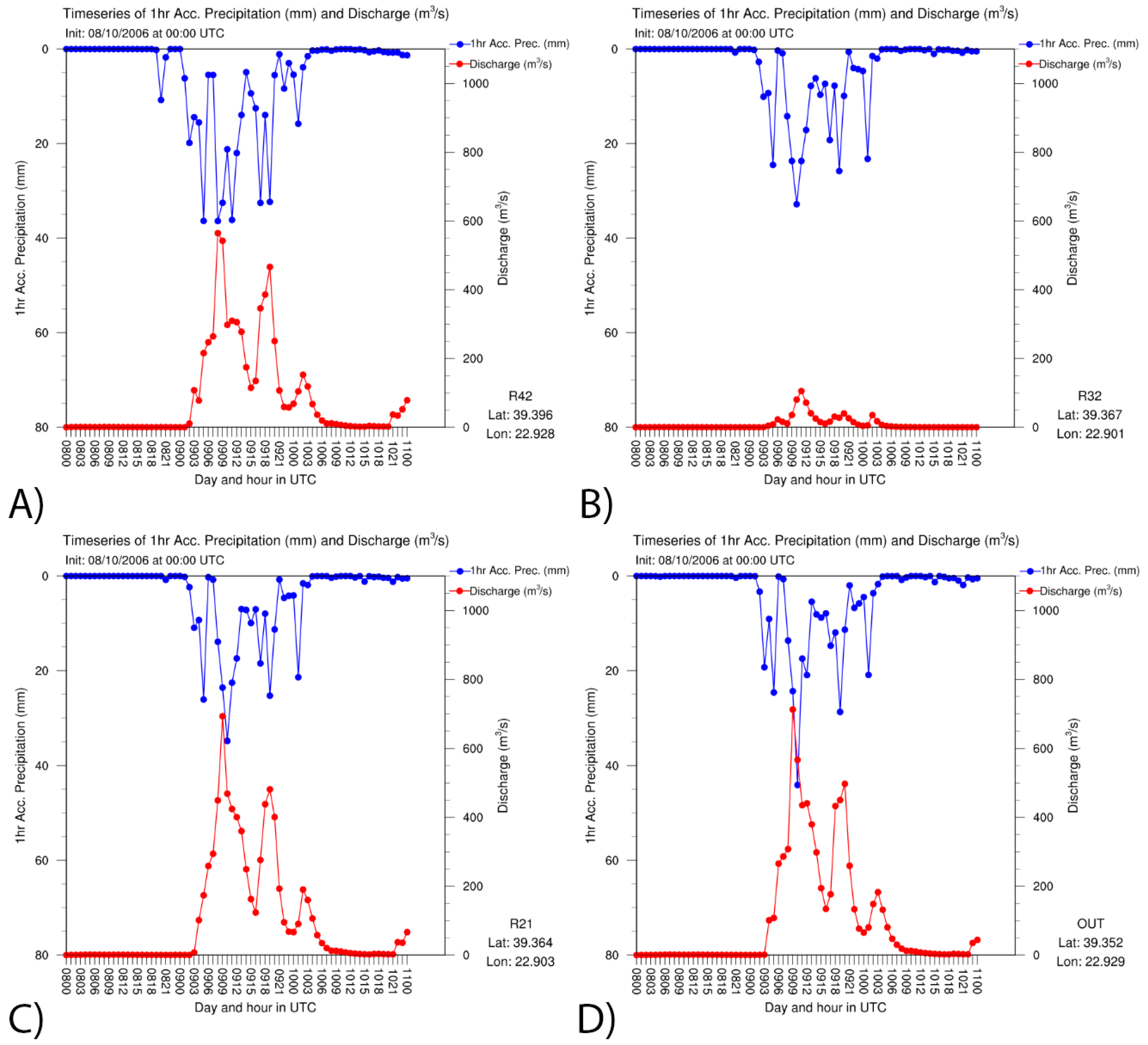
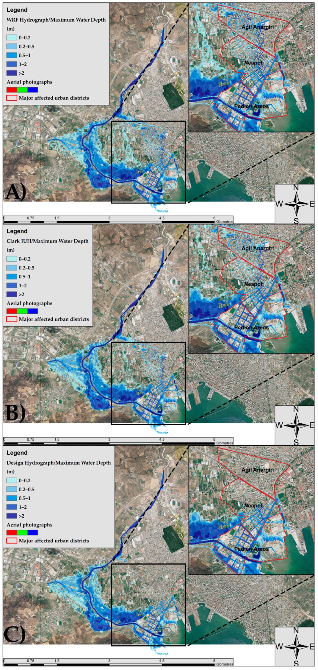
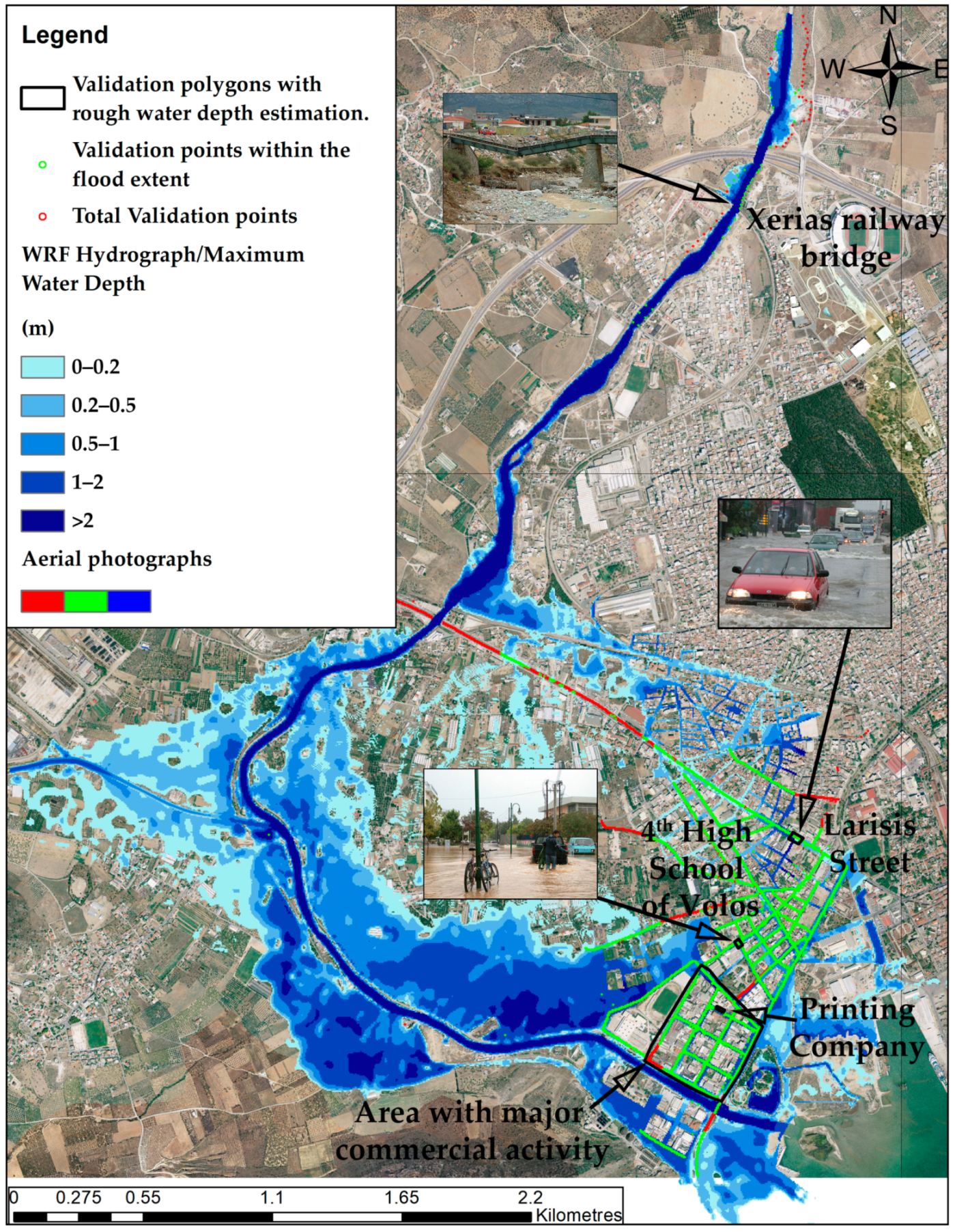
• Hydrographs generated from the combined weather–hydrological model presented in Section 3.1. These flood hydrographs are named from now on as “WRF hydrograph”.
• Hydrographs based on previous studies [5,6,10,35,73]. These hydrographs were generated based on the Clark Instantaneous Unit Hydrograph and the use of Kinematic wave approximation. They are named from now on as “Clark IUH”.
• Design hydrographs based on a previous study [5]. The design hydrographs are estimated for the return period of 100 years (T = 100 years) and the second type of antecedent soil moisture conditions (AMC_II). These hydrographs are named from now on as “Design Hydrograph”.

Other important characteristics of the HEC-RAS 2D model configuration are: (1) The average flexible mesh computation point spacing is 14 m (variable and smaller point spacing was used around the bridges and the urban areas to accurately depict the hydraulic structures and the road network); (2) breaklines that represent the main stream, the banks, the hydraulic structures (e.g., bridges), and the Volos city building blocks were used to generate cells that align with the breaklines; (3) 2D diffusion wave solution was used for the simulation; (4) the computation interval was set to two (2) seconds; and (5) all Volos city building blocks were represented with a 30 m local increase of the elevation (elevation rise method) (Figure 1D).

The results derived from all of the hydraulic model sub-domains were merged in order to retrieve the maximum water depth and the flood extent in the study area (Figure 1D). As described in Section 2.2, validation point data were extracted based on the flood data collection for the validation of the simulations. Since the study area was characterised by lack of any gauged data and other flood-related measurements, the primary focus of the validation process is the flood extent. In particular, the accuracy of the simulated flood extent was evaluated by calculating the percentage of the validation data located within the simulated flood extent. In order to provide more quantitative insights on the model performance, four (4) water depth observations extracted from photographs taken after the event and from local mass media reports were inserted in the validation analysis (Figure 2, polygons and photos n.1–n.4). The obtained water depths were not defined as point observations, but they were assigned to wider areas based on the coverage of the floodwater illustrated in the selected photographs and the press reports. These areas were used to delineate specific polygons, in which the median values of the simulated water depths were calculated to be comparable with the corresponding flood observations.

3. Results

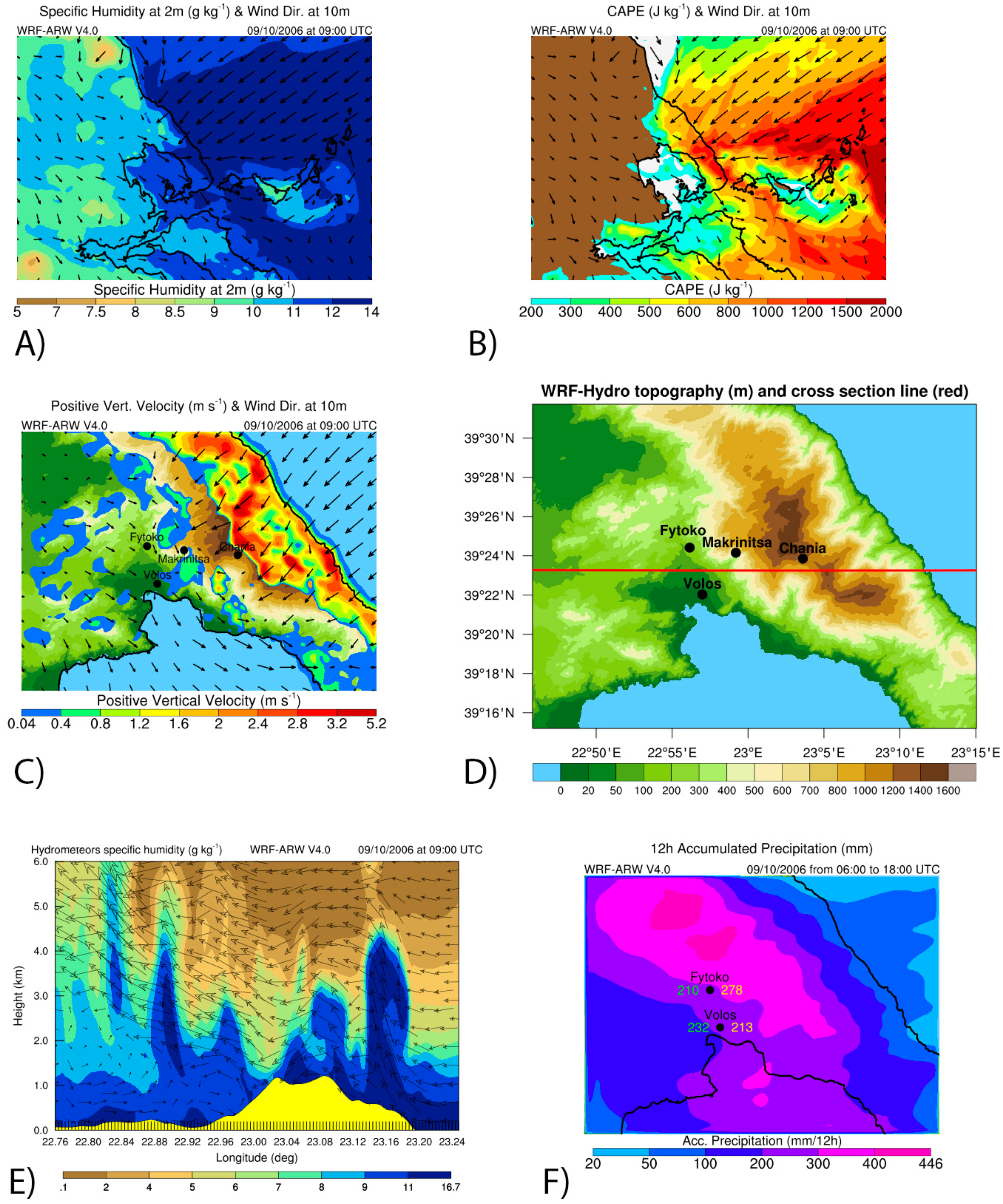
3.1. Hydrometeorological Analysis

The flood event in Volos city was associated with a severe storm caused by a very slowly moving barometric low over the Aegean Sea, supported by an upper air trough [44]. The synergy between the prevailed synoptic conditions and the orographic convergence of unstable air over Pelion mountain developed a persistent storm, characterised by torrential rainfall.

In more detail, on 8 October at 06:00 UTC, a cold upper air trough (500-hPa level) moved from central Europe southward to the Mediterranean Sea, supporting the formation of a barometric low over Greece centred over the Aegean Sea (Figure 5A). The upper air temperature in the core of the trough over southern Italy was about −18 °C, quite lower than the surrounding areas. Six hours later, at 12:00 UTC, the southeastward movement of the trough triggered deepening of the barometric low, which reached a minimum MSL pressure of 1008 hPa (Figure 5B). The combination of low atmospheric pressures over Greece, with an anticyclonic (high atmospheric pressure) system over central Europe, provoked isobar thickening over the central Balkan Peninsula and, subsequently, enhanced near-surface easterly winds over this area (Figure 5A,B). At 18:00 UTC, the trough, continuing the slow southeastward movement, was isolated from the western atmospheric circulation and it was finally cut off (Figure 5C). The cutoff of the trough was critical for the evolution of the barometric low and, subsequently, for the severe storm causing the flash flood. The isolation of middle and upper air from the main western circulation, which can cause the formation of cutoff troughs, is often associated with extreme weather events characterised by heavy rainfall [13,74,75]. The studied cutoff trough preserved its characteristics, like positive vorticity (not shown) and low temperature, offering favourable conditions to the barometric low staying in place for many hours.

On 9 October, during the period from 00:00 UTC to 12:00 UTC, the cutoff trough slowly moved to the Ionian Sea and regional Greece, supporting the displacement of the barometric low to the southern Aegean Sea and the formation of a secondary barometric low over the southern Ionian Sea (Figure 5D–F). During the same period, the high-pressure barometric system over central Europe was intensified by a relatively warmer ridge (500 hPa), which originated from the western Mediterranean Sea, and as a result, MSL pressure reached 1026 hPa at its centre. Under these atmospheric conditions, high pressures were favoured to expand to the Balkan Peninsula, while low pressures remained dominant over southern Greece. The balance of these adverse conditions pushed the thick-isobar area, characterised by high-pressure gradients and intense easterly winds, to move from the central Balkans to the Aegean Sea. The easterly winds over the Aegean Sea transferred moist and unstable air to the wider area of Pelion mountain over Volos city.

Figure 6A,B presents the advection of air characterised by specific humidity of 12–14 g kg⁻¹ and convective available potential energy (CAPE) of 800–1200 J kg⁻¹ towards the windward side of Pelion mountain on 9 October at 09:00 UTC. This upwind airflow orographically lifted over the mountain, as shown by the positive vertical velocities reaching 5.2 m s⁻¹ (Figure 6C). The moist and unstable updrafts over Pelion and Volos, as shown by the vertical cross-section illustration of Figure 6D–F, generated water-rich clouds with specific humidity up to 16.7 g kg⁻¹. These conditions led us to conclude that the buildup of moisture and CAPE in the updrafts over the precise area for several hours drove to the evolution of the persistent storm. The combination of the orographic convergence of humid–unstable air originated from the Aegean Sea, with the approaching cutoff trough accompanied by positive vorticity and reduced geopotential heights, favoured the enhancement of atmospheric instability, which caused the severe storm.

It is noteworthy that during the period from 06:00 to 18:00 UTC on 9 October, the model estimated precipitation of 213 mm and 446 mm in Volos city and at Pelion mountain peaks, respectively. This amount of precipitation in only 12 h is considered as extreme because it approximately corresponds to the annual accumulated precipitation of Volos city, which varies from 400 to 770 mm, based on data retrieved from the meteorological station of Volos city in the network of the National Observatory of Athens (NOA) with operation period from February 2007 to July 2017. Indeed, the local news talked about a “nonstop” rainfall that lasted from 10:00 local time until the late evening of the same day, creating chaos in the main city of Volos and the surroundings. The authorities characterised the rainfall event as the highest in duration and intensity within the last twelve years and issued the prefecture of Magnesia in an emergency state. The model results indicate an overestimation in comparison with measurements at Fytoko meteorological station (Source: Institute of Industrial Plants and Livestock—Department of Plant Protection, Volos) [10]. The measured precipitation from 06:00 to 18:00 UTC at Fytoko station was 210 mm [10,73]; however, the model estimated about 278 mm in the same area. On the other hand, the model estimated precipitation of 213 mm in Volos city during the same period, presenting a small underestimation in comparison with the measured precipitation of 232 mm [44]. These differences between spatially averaged model-generated (over a grid area) and the measured point-values are the results of sub-grid scale atmospheric processes during such severe phenomena and the various errors introduced in measurements and simulations.

The results of hydrometeorological simulations of the flash flood event in Volos city are presented in this section. Discharge simulated by the WRF-Hydro model at 01:00, 08:00, 09:00, and 18:00 UTC of 9 October is shown in Figure 7A–D, superimposed by the corresponding 1-h accumulated precipitation (mm) simulated by the WRF-ARW model. Figure 7 presents different characteristics in the spatial pattern and intensities for the four different times. Figure 7A presents the beginning of the event at the Pelion mountain slopes, while Figure 7B,C show the peak of the flash flooding reaching precipitation rates of 84 mm h⁻¹ and discharge of 715 m³ s⁻¹. Moreover, Figure 7D demonstrates the second peak of the storm, re-triggering the flash flooding during the evening, with precipitation rates exceeding 40 mm h⁻¹ over Xerias drainage basin, while discharge reaching 350 m³ s⁻¹. Afterwards, discharge presents a higher peak of 497 m³ s⁻¹ at 20:00 UTC. The differences in maps are attributed to the different mature stages of orographic lifting of warm and humid air masses originating from the Aegean Sea, following the easterly atmospheric flow which was induced by the almost stagnant barometric low. It is noteworthy that the spatiotemporal distribution of precipitation affects the available surface and soil moisture determining surface- and channel-water runoff and, therefore, the streams’ routing. Figure 8 presents the hydrologic response of Xerias watershed for the extreme storm event of 9 October 2006 at the locations (A) R42 (Upper Xerias sub-watershed), (B) R32 (Seskouliotis and Kakaviotis sub-watershed), (C) R21, and (D) OUT (Xerias Watershed outlet). These flood hydrographs were used as an input boundary condition in the 2D HEC-RAS hydraulic–hydrodynamic model for river flood modelling.

Table 3. Maximum discharge (m³ s⁻¹) values of all the examined flood hydrographs used as input to the hydraulic–hydrodynamic model at junctions R42, R32, and R21.

Junction	Maximum Discharge (m3 s−1) Values
	WRF Hydrograph	Clark IUH	Design Hydrograph
R42	564.6	490.43	385.72
R32	105.2	204.41	160.79
R21	692.8	681.89	536.31

demonstrates the maximum discharge values of all examined flood hydrographs used as input to the hydraulic–hydrodynamic model at junctions R42, R32, and R21. In comparison to the other two flood hydrographs (i.e., Clark IUH and Design Hydrograph), WRF-based hydrograph yielded a lower maximum discharge value at R32 and a higher one at R42. This is attributed to the capability of the WRF-ARW weather simulation to physically represent the inhomogeneous pattern of precipitation across the watershed. However, the other two approaches distribute equally the precipitation over the study area. Hence, the spatial differences in precipitation affect the results of the WRF-hydro hydrological simulation, leading to higher discharge values at R42 due to heavy rainfall at Pelion mountain and lower discharge values at R32 which was partly covered by the storm.

3.2. Hydraulic Simulation Results

Figure 9 presents the maximum water depths and the flood extent simulated by the 2D flood inundation model using three different boundary conditions for each junction point (R42, R32, R21) of Xerias river: (A) WRF hydrograph, (B) Clark IUH, and (C) design hydrograph. Τhe spatial distribution of the simulated flood extent reveals that the results derived from the WRF hydrograph coincide with the spatial pattern obtained using the Clark IUH. Both simulations depict major flooding in the areas expanding west of Volos Port along Xerias torrent, indicating particularly high local values within Agii Anargiri, Neapoli, and Pedion Areos areas (framed areas in Figure 9A,B). However, this is not the case for the design hydrograph, which fails to capture localised flooding, especially in Agii Anargiri area (Figure 9C). Design hydrograph was not generated for the specific event but for a designed flood of 100 years and, as a result, the simulated maximum discharge value in junction R42 is lower than the maximum flow peaks of the other two hydrographs (i.e., WRF hydrograph and Clark IUH). The aggregated scores derived from the validation process for the three flood hydrographs are detailed in

Table 4. Validation statistics for all examined flood extent based on the flood hydrographs used.

Validation Points within the Flooded Area	Flood Hydrographs
	WRF Hydrograph	Clark IUH	Design Hydrograph
Number of points	3559	3367	2456
Percentage (%)	84	79	58

. In general, all of the study simulations manage to provide acceptable scores based on the percentage of validation points that fall within the simulated flood extent. WRF hydrograph produces the highest success rate score with 84% of the validation points to be observed within the simulated flood extent. As expected, the WRF physically-based approach provides the best correspondence with the observed flooded area and, therefore, its results are considered as more “accurate” than the ones of the other methods. These results will be further discussed and compared with the qualitative data of Section 2.2. Nevertheless, it is important to point out that despite the difference between the WRF hydrograph and the Clark IUH validation scores, Clark IUH achieves high success rate scores as well (79%).

The cumulative distribution functions of the simulated water depth calculated for the three flooded areas, separately, show that WRF and Clark IUH simulations converge to maximum water depths of about 2.2 m (Figure 10). Indeed, qualitative analysis of the local press indicated cases in which floodwaters reached large values, around or even higher than 2 m, creating major catastrophes to the infrastructure of Agii Anargiri and Neapoli areas. Characteristically, mass-media and press reports mentioned that residents and business owners in Agii Anargiri and Neapoli were desperate, trying to clean their property from mud and floodwaters, which sometimes exceeded 1.5 m until the next evening on 10 October. Based on the WRF-based simulations, the median values of the maximum water depths were estimated as 0.43 m, 0.67 m, and 0.63 m in Agii Anargiri, Neapoli, and Pedion Areos, respectively (Figure 10). U.S. Federal Emergency Management Agency (FEMA) estimates that 0.3 m of flash flood water could float many vehicles, whereas 0.6 m of rushing water could carry away most vehicles, including SUVs and pickups. In Neapoli and Pedion Areos, the fire services undertook multiple emergency calls from 21 recorded flooded roads. Although flood velocity is the primary determinant for incidents to motorists, the simulated floodplain gives a strong indication of the vulnerable roads, which concentrated a mass of validation points. In Figure 11, it is apparent that the incidents reported by the Fire Department shape the dense road network of the commercial area (green points in Figure 11), and they are indicative of the high exposure of citizens during the active commercial hours of a weekday that the event occurred. In addition to that, flooding caused the roads of Volos to get overloaded with private and public vehicles, as well as hundreds of taxis that attempted to drive people to their relatives and properties. In times of crisis, people consider their place as a safe destination where “nothing bad can happen” or as the reference point where the family gathers for a collective response in case of emergency [76]. There were many cases in the past in which individuals lost their lives in their effort to reach a destination like home or while attempting to retrieve their belongings and pets from flooded buildings [77,78].

In the flood event of 9 October, the Traffic Police of Volos struggled to deal with dozens of stranded cars and to coordinate the traffic jams across the city. Unfortunately, the lack of detailed flood records on the validation points does not allow for a thorough comparison with the simulated water depths on the road network. A rough estimation of the flood water depth was possible only to certain locations which were detailed in the press or to which relevant pictures could be assigned based on the knowledge of the authors. From the stranded cars pictured on the green dots in Figure 11, the authors estimate water depth around 0.5 m in Larisis Street, which crosses Neapoli and Agii Anargiri areas. This is to be compared with the 0.8 m extracted as the median value of the simulated maximum depths in the validation polygon of Larisis street (Figure 11). Traffic also increased as municipality services started to transfer students from flooded schools to their homes late in the morning on Monday 9 October. Many schools in central Volos City and the Prefecture of Magnesia were evacuated and remained closed the next day. The authors managed to associate a picture collected in the validation data with the location of a flooded school in Neapoli (4th high school of Volos city) to get an indicative value of the observed water depth. WRF simulations present a median value of 0.78 m that is slightly higher than the 0.4–0.5 m assessed from the corresponding image (see Figure 11). Slight overestimations could be attributed to the fact that the observed water depth data do not correspond to the maximum levels reached in the current event because of the differences between the timing of the simulated water depth and the actual timing that the photo was taken. It should be noted that flash floods are characterised by a sharp rise followed by a relatively rapid decline, causing high flow velocities. In flash floods, discharge quickly reaches a maximum level and diminishes almost as rapidly [79].

The validation points also include a bunch of emergency calls (more than three hundred) from residents who asked for help in flooded homes and stores from 07:00 UTC (10:00 local time) and after on 9 October, and especially after noon in Neapoli, following the hydrologic peaks presented in the previous section. However, there are no witnesses about the depth of floodwaters in these locations to assess the average situation in the flooded areas. In the commercial area that extends north of Neapoli to Pedion Areos, the media refer to floodwaters reaching 1.5 m and immobilising owners inside their stores. In accordance with this statement, the WRF simulations give a median of 1.21 m in the validation polygon that corresponds to the main commercial area affected by the floodwaters. Notably, 80% of the companies that claimed compensation for flood damages to the Greek government are located in this polygon (see validation polygons in Figure 11). One of the largest printing companies, which was highly affected by the flood in this area, serves as an additional validation point (Figure 11). The press highlighted that the building was completely destroyed, with floodwaters exceeding 1.5 m. WRF-based simulations provide a good approximation in this spot, with a median water depth of 1.68 m in the validation polygon that surrounds the structure (see Printing company in Figure 11). The model gives particularly high values in some locations in Upper Volos. In that area, the iron railway bridge at Xerias intersection collapsed at 13:00 UTC (16:00 local time) due to the significant volume of floodwater from Xerias torrent and the intense debris flow hitting its foundations (bridge shown in Figure 11). WRF-simulated water depths reached maximum values as high as 4 m at the flood peak around the bridge. Although interviewed locals mentioned that floodwaters overcame the bridge, the local press reported about 2 m of water, and it is probably a more reliable source of information. An overestimation of this value could be related to the exceptional conditions generated by the debris flow (i.e., carried cobbles, boulders, olive trees, and mud) at the preceding bridge, leading to lower water depths with higher flow velocities at the location of the railway bridge. Despite the unavoidable uncertainties on the exact values, it appears that the simulations provide valuable indications about the harshness of the situation. As a result of the catastrophic event, the national railway was interrupted, disconnecting Volos from the rest of the country for many weeks after the event. Given that the event occurred during the morning rush hours, it is fortunate that, after the intervention of local residents, authorities discontinued the train schedule between Larisa and Volos just before the bridge collapsed. This measure prevented possible accidents and losses of human lives.

4. Concluding Remarks

The interaction between the atmosphere and the hydrosphere defines the water cycle, and sometimes favours extreme weather phenomena like flash floods, which impact human health and economy. Interdisciplinary multi-scale and multi-model systems are needed to simulate flash flood events because of the high spatiotemporal connections of complex interactive socio-hydrometeorological phenomena. This study proposes the use of coupled weather, hydrological, and hydraulic models for river flood modelling and mapping at ungauged catchments, simulating a historical flood event that occurred on 9 October 2006 in Volos city, Greece. In the first part of our methodology, the meteorological approach used nesting techniques (using five nested domains) reaching a very fine horizontal resolution (250 × 250 m) on the fifth domain in order to resolve orographic and cloud microphysical effects that define the location and the intensity of the storm. In the second part, the hydrological approach effectively represented the soil processes and surface runoff routing. The hydrological model was set up on the extent of the fifth domain of the meteorological model, including the drainage basin of Xerias stream on the five-times finer horizontal resolution of 50 × 50 m. The methodology was completed with hydraulic–hydrodynamic modelling that applies standard hydraulic modelling parameterisation techniques for ungauged catchments. Several conventional and unconventional flood-related data (e.g., damage estimation reports, photographs, local mass-media reports, and interviews with eyewitnesses) were collected and incorporated in the analysis to better understand the extreme flash flood event, as well as to generate an indicative validation dataset for the flood simulations. Flood inundation modelling and mapping was produced based on the flood hydrographs generated by the current analysis, as well as in prior studies [5,6,10,35,73]. Due to severe lack of observational data, flood extent was the main criterion used for the verification of the hydraulic–hydrodynamic simulations presented in this work. The validation process of the flood extent was accomplished by estimating the percentage of validation data observed within the simulated flood extent divided by the total number of validation data. To expound this analysis and to examine the model performance in terms of water depth simulation, relevant photos and press documentary were used to assess the observed water depths in four possible locations. The water depth assessments were assigned to four polygons, respectively, based on the extent of floodwater of given depth illustrated on the selected photographs or discussed in the local mass media reports. This allowed for a rough comparison between the observed water depths and the median values of the simulated water depths that belonged to the specified polygons.

The meteorological simulation results indicated a severe persistent storm over Pelion mountain at the northeast of Volos city as the main factor of the flash flood event. The orographic convergence of easterly airflow, rich in moisture and convective available potential energy that originated from the Aegean Sea, was the dominant parameter for the evolution of the storm. The simulated precipitation rates reached 84 mm/h at the peak of the storm. The hydrological simulation resulted in the maximum discharge of about 715 m³ s⁻¹ in Xerias stream, which mainly caused the flash flooding.

The proposed physically-based approach for the flood hydrograph generation proved to be the most efficient among the three examined flood hydrographs and the corresponding flood extents (WRF hydrograph validation score is 84%). It is noteworthy to mention that the Clark IUH, which was generated based on the relationship between the hydrological characteristics of the watershed and the geomorphologic parameters, was illustrated efficiently the hydrological behaviour of the examined flood event as well (Clark IUH validation score is 79%). Furthermore, the WRF hydrograph provided a good approximation of the water depth within the four water depth validation spots. Our experiments were in complete agreement with previous works that estimated the return period of the 2006 flash flood event to approximately 100 years [5,6,10,35,73]. Unfortunately, there was no official flood dataset allowing for the detailed validation of critical flood characteristics, such as the observed water depth, the speed of the flood, and its subsequent catastrophes for the event of 9 October 2006 in Volos city. Though, empirical evidence obtained after processing information from local authorities and the press demonstrates correspondence between the highest values of the simulated water depth with the most impacted locations. Results presented in this study further strengthen our confidence in using physically-based approaches, especially at ungauged watersheds, for flood hydrograph generation of case study events and flood inundation modelling and mapping.

Such flood mapping may serve as an indication of the environmental and human exposure in future flood events in Volos to warn for potential agricultural losses or structural damages and human losses in rural and urban areas, respectively. Volos Municipality and the Prefecture of Magnesia could use this information to develop local or regional strategies for flood risk mitigation including: (1) Structural measures for the prevention of waters in the most flood-prone areas across Xerias torrent, (2) relevant legislation and insurance policy for properties and businesses in flood-prone zones, and (3) educational campaigns for residents and workers to increase flood risk awareness in densely occupied neighbourhoods or locations of particular use (e.g., commerce, fishery). The current study could be ultimately expanded to propose a methodological framework to support early warning systems for flood hazards in Europe. Recent studies have suggested the integration of weather and discharge forecasts identical with the ones estimated in this work with exposure characteristics of individuals and infrastructures for a holistic, dynamic risk modelling that translates hydrometeorological forecasts into impact-based predictions [18,80]. In this direction, discharge simulations can further improve river modelling to estimate hydraulic characteristics (i.e., water depth, velocity, water or flood extent) which can inform civil protection agencies about dangerous spots for intervention when combined with the societal vulnerabilities that emerge at the time of the event.

References

1. Centre for Research on the Epidemiology of Disasters (CRED). Summarized Table of Natural Disasters in Europe from 1900 to 2019, EM-DAT: The CRED/OFDA International Disaster Database–www.emdat.be–Université Catholique de Louvain–Brussels–Belgium. Available online: http://www.emdat.be (accessed on 31 July 2019).
2. Gangrade, S.; Kao, S.C.; Dullo, T.T.; Kalyanapu, A.J.; Preston, B.L. Ensemble-Based flood vulnerability assessment for probable maximum flood in a changing environment. J. Hydrol. 2019, 576, 342–355. [Google Scholar] [CrossRef]
3. Hall, J.; Arheimer, B.; Borga, M.; Brázdil, R.; Claps, P.; Kiss, A.; Kjeldsen, T.R.; Kriaučiūnienė, J.; Kundzewicz, Z.W.; Lang, M.; et al. Understanding flood regime changes in Europe: A state-of-the-art assessment. Hydrol. Earth Syst. Sci. 2014, 18, 2735–2772. [Google Scholar] [CrossRef]
4. Zeleňáková, M.; Gaňová, L.; Purcz, P.; Horský, M.; Satrapa, L.; Blišťan, P.; Diaconu, D.C. Mitigation of the Adverse Consequences of Floods for Human Life, Infrastructure, and the Environment. Nat. Hazards Rev. 2017, 18, 1–15. [Google Scholar] [CrossRef]
5. Papaioannou, G.; Efstratiadis, A.; Vasiliades, L.; Loukas, A.; Papalexiou, S.; Koukouvinos, A.; Tsoukalas, I.; Kossieris, P. An Operational Method for Flood Directive Implementation in Ungauged Urban Areas. Hydrology 2018, 5, 24. [Google Scholar] [CrossRef]
6. Papaioannou, G.; Loukas, A.; Vasiliades, L.; Aronica, G.T. Flood inundation mapping sensitivity to riverine spatial resolution and modelling approach. Nat. Hazards 2016, 83, 117–132. [Google Scholar] [CrossRef]
7. Macchione, F.; Costabile, P.; Costanzo, C.; De Lorenzo, G. Extracting quantitative data from non-conventional information for the hydraulic reconstruction of past urban flood events. A case study. J. Hydrol. 2019, 576, 443–465. [Google Scholar] [CrossRef]
8. Aronica, G.T.; Franza, F.; Bates, P.D.; Neal, J.C. Probabilistic evaluation of flood hazard in urban areas using Monte Carlo simulation. Hydrol. Process. 2012, 26, 3962–3972. [Google Scholar] [CrossRef]
9. Kiczko, A.; Mirosław-Świątek, D. Impact of Uncertainty of Floodplain Digital Terrain Model on 1D Hydrodynamic Flow Calculation. Water 2018, 10, 1308. [Google Scholar] [CrossRef]
10. Papaioannou, G. Flood Hazard and Risk Modelling Framework for Ungauged Streams and Watersheds; University of Thessaly: Volos, Greece, 2017. [Google Scholar]
11. Teng, J.; Jakeman, A.J.; Vaze, J.; Croke, B.F.W.; Dutta, D.; Kim, S. Flood inundation modelling: A review of methods, recent advances and uncertainty analysis. Environ. Model. Softw. 2017, 90, 201–216. [Google Scholar] [CrossRef]
12. Apel, H.; Aronica, G.T.; Kreibich, H.; Thieken, A.H. Flood risk analyses—How detailed do we need to be? Nat. Hazards 2009, 49, 79–98. [Google Scholar] [CrossRef]
13. Varlas, G.; Anagnostou, M.N.; Spyrou, C.; Papadopoulos, A.; Kalogiros, J.; Mentzafou, A.; Michaelides, S.; Baltas, E.; Karymbalis, E.; Katsafados, P. A multi-platform hydrometeorological analysis of the flash flood event of 15 November 2017 in Attica, Greece. Remote Sens. 2019, 11, 45. [Google Scholar] [CrossRef]
14. Skamarock, W.C.; Klemp, J.B.; Dudhia, J.; Gill, D.O.; Barker, D.M.; Duda, M.G.; Huang, X.-Y.; Wang, W.; Powers, J.G. A Description of the Advanced Research WRF Version 3. NCAR Tech. NOTE—NCAR/TN-475+STR; UCAR: Boulder, CO, USA, 2008; Volume 125. [Google Scholar] [CrossRef]
15. Powers, J.G.; Klemp, J.B.; Skamarock, W.C.; Davis, C.A.; Dudhia, J.; Gill, D.O.; Coen, J.L.; Gochis, D.J.; Ahmadov, R.; Peckham, S.E.; et al. The weather research and forecasting model: Overview, system efforts, and future directions. Bull. Am. Meteorol. Soc. 2017, 98, 1717–1737. [Google Scholar] [CrossRef]
16. Gochis, D.J.; Barlage, M.; Dugger, A.; Fitzgerald, K.; Karsten, L.; McAllister, M.; McCreight, J.; Mills, J.; RafieeiNasab, A.; Read, L.; et al. The WRF-Hydro modeling system technical description (Version 5.0); NCAR Technical Note; National Center for Atmospheric Research: Boulder, CO, USA, 2018; p. 107. [Google Scholar]
17. Senatore, A.; Mendicino, G.; Gochis, D.J.; Yu, W.; Yates, D.N.; Kunstmann, H. Fully coupled atmosphere-hydrology simulations for the central Mediterranean: Impact of enhanced hydrological parameterization for short and long time scales. J. Adv. Model. Earth Syst. 2015, 7, 1693–1715. [Google Scholar] [CrossRef]
18. Silvestro, F.; Rossi, L.; Campo, L.; Parodi, A.; Fiori, E.; Rudari, R.; Ferraris, L. Impact-Based flash-flood forecasting system: Sensitivity to high resolution numerical weather prediction systems and soil moisture. J. Hydrol. 2019, 572, 388–402. [Google Scholar] [CrossRef]
19. Givati, A.; Gochis, D.; Rummler, T.; Kunstmann, H. Comparing One-Way and Two-Way Coupled Hydrometeorological Forecasting Systems for Flood Forecasting in the Mediterranean Region. Hydrology 2016, 3, 19. [Google Scholar] [CrossRef]
20. Sanz-Ramos, M.; Amengual, A.; Bladé, E.; Romero, R.; Roux, H. Flood forecasting using a coupled hydrological and hydraulic model (based on FVM) and highresolution meteorological model. EDP Sciences 2018, 40, 1–8. [Google Scholar] [CrossRef]
21. Zhu, X.; Dai, Q.; Han, D.; Zhuo, L.; Zhu, S.; Zhang, S. Modeling the high-resolution dynamic exposure to flooding in a city region. Hydrol. Earth Syst. Sci. 2019, 23, 3353–3372. [Google Scholar] [CrossRef] [Green Version]
22. Afifi, Z.; Chu, H.J.; Kuo, Y.L.; Hsu, Y.C.; Wong, H.K.; Ali, M.Z. Residential flood loss assessment and risk mapping from high-resolution simulation. Water (Switzerland) 2019, 11, 751. [Google Scholar] [CrossRef]
23. Langhammer, J.; Lendzioch, T.; Miřijovskỳ, J.; Hartvich, F. UAV-Based optical granulometry as tool for detecting changes in structure of flood depositions. Remote Sens. 2017, 9, 240. [Google Scholar] [CrossRef]
24. Kiczko, A.; Romanowicz, R.J.; Osuch, M.; Karamuz, E. Maximising the usefulness of flood risk assessment for the river Vistula in Warsaw. Nat. Hazards Earth Syst. Sci. 2013, 13, 3443–3455. [Google Scholar] [CrossRef]
25. Jalayer, F.; Aronica, G.T.; Recupero, A.; Carozza, S.; Manfredi, G. Debris flow damage incurred to buildings: An in situ back analysis. J. Flood Risk Manag. 2018, 11, S646–S662. [Google Scholar] [CrossRef]
26. Gourley, J.J.; Flamig, Z.L.; Vergara, H.; Kirstetter, P.E.; Clark, R.A.; Argyle, E.; Arthur, A.; Martinaitis, S.; Terti, G.; Erlingis, J.M.; et al. The flash project Improving the Tools for Flash Flood Monitoring and Prediction across the United States. Bull. Am. Meteorol. Soc. 2017, 98, 361–372. [Google Scholar] [CrossRef]
27. Martinaitis, S.M.; Gourley, J.J.; Flamig, Z.L.; Argyle, E.M.; Clark, R.A.; Arthur, A.; Smith, B.R.; Erlingis, J.M.; Perfater, S.; Albright, B. The hmt multi-radar multi-sensor hydro experiment. Bull. Am. Meteorol. Soc. 2017, 98, 347–359. [Google Scholar] [CrossRef]
28. Gaume, E.; Borga, M. Post-Flood field investigations in upland catchments after major flash floods: Proposal of a methodology and illustrations. J. Flood Risk Manag. 2008, 1, 175–189. [Google Scholar] [CrossRef]
29. Brunner, G.W. CEIWR-HEC HEC-RAS River Analysis System 2D Modeling User’s Manual; US Army Corps of Engineers—Hydrologic Engineering Center: Davis, CA, USA, 2016. [Google Scholar]
30. Koutsogiannis, D.; Markonis, I. Hydrological Analysis of Xerias River Basin, Magnesia—Flood Works Report of Xerias, Seskouliotis and Kakaviotis Streams; Magnesia Prefectural Authority and Mahairas Technical Consultant Company: Athens, Greece, 2010. (in Greek) [Google Scholar]
31. Hellenic Statistical Authority. 2011 POPULATION AND HOUSING CENSUS Demographic and Social Characteristics of the Resident Population of Greece according to the 2011 Population—Housing Census Revision of 20/3/2014; Hellenic Statistical Authority: Piraeus, Greece, 2014. [Google Scholar]
32. Diakakis, M.; Mavroulis, S.; Deligiannakis, G. Floods in Greece, a statistical and spatial approach. Nat. Hazards 2012, 62, 485–500. [Google Scholar] [CrossRef]
33. Special Secretariat for Water, M. of E. and E. (SSW-M. Preliminary Assessment of the Flood Directive; Athens: Ministry of Environment and Energy. Available online: http://www.ypeka.gr/Lin%0AkClick.aspx?fileticket=T4DDG1hqQMY%3D&tabid=252&language=el-GR%0A (accessed on 1 July 2019).
34. Papaioannou, G.; Vasiliades, L.; Loukas, A. Multi-Criteria Analysis Framework for Potential Flood Prone Areas Mapping. Water Resour. Manag. 2015, 29, 399–418. [Google Scholar] [CrossRef]
35. Papaioannou, G. Sensitivity analysis of a probabilistic flood inundation mapping framework for ungauged catchments. Eur. Water 2017, 9–16. [Google Scholar]
36. Shepherd, M.; Mote, T.; Dowd, J.; Roden, M.; Knox, P.; McCutcheon, S.C.; Nelson, S.E. An overview of synoptic and mesoscale factors contributing to the disastrous Atlanta flood of 2009. Bull. Am. Meteorol. Soc. 2011, 92, 861–870. [Google Scholar] [CrossRef]
37. Varlas, G.; Papadopoulos, A.; Katsafados, P. An analysis of the synoptic and dynamical characteristics of hurricane Sandy (2012). Meteorol. Atmos. Phys. 2018, 131, 1–11. [Google Scholar] [CrossRef]
38. Katsafados, P.; Varlas, G.; Papadopoulos, A.; Spyrou, C.; Korres, G. Assessing the Implicit Rain Impact on Sea State During Hurricane Sandy (2012). Geophys. Res. Lett. 2018, 45, 12015–12022. [Google Scholar] [CrossRef]
39. Christakos, K.; Varlas, G.; Reuder, J.; Katsafados, P.; Papadopoulos, A. Analysis of a low-level coastal jet off the Western coast of Norway. Energy Procedia 2014, 53, 162–172. [Google Scholar] [CrossRef]
40. Christakos, K.; Cheliotis, I.; Varlas, G.; Steeneveld, G.J. Offshore Wind Energy Analysis of Cyclone Xaver over North Europe. Energy Procedia 2016, 94, 37–44. [Google Scholar] [CrossRef] [Green Version]
41. Varlas, G.; Katsafados, P.; Papadopoulos, A.; Korres, G. Implementation of a two-way coupled atmosphere-ocean wave modeling system for assessing air-sea interaction over the Mediterranean Sea. Atmos. Res. 2018, 208, 201–217. [Google Scholar] [CrossRef]
42. Varlas, G.; Katsafados, P.; Korres, G.; Papadopoulos, A. Assessing the impact of Argo floats temperature measurements on the numerical weather prediction forecast skill of a weather prediction numerical model. Mediterr. Mar. Sci. 2019, 20, 331–334. [Google Scholar] [CrossRef]
43. Cheliotis, I.; Varlas, G.; Christakos, K. The Impact of Cyclone Xaver on Hydropower Potential in Norway. In Perspectives on Atmospheric Sciences; Karacostas, T., Bais, A., Nastos, P.T., Eds.; Springer International Publishing: Cham, Switzerland, 2017; pp. 175–181. ISBN 978-3-319-35095-0. [Google Scholar]
44. Harats, N.; Ziv, B.; Yair, Y.; Kotroni, V.; Dayan, U. Lightning and rain dynamic indices as predictors for flash floods events in the Mediterranean. Adv. Geosci. 2010, 23, 57–64. [Google Scholar] [CrossRef] [Green Version]
45. Creutin, J.D.; Borga, M.; Gruntfest, E.; Lutoff, C.; Zoccatelli, D.; Ruin, I. A space and time framework for analyzing human anticipation of flash floods. J. Hydrol. 2013, 482, 14–24. [Google Scholar] [CrossRef]
46. Danielson, J.J.; Gesch, D.B. Global multi-resolution terrain elevation data 2010 (GMTED2010); US Geological Survey: Reston, VA, USA, 2011.
47. Myneni, R.; Hoffman, S.; Knyazikhin, Y. Global products of vegetation leaf area and fraction absorbed PAR from one year of MODIS data. Remote Sensing of. Environment 2002, 76, 139–155. [Google Scholar]
48. Friedl, M.A.; Sulla-Menashe, D.; Tan, B.; Schneider, A.; Ramankutty, N.; Sibley, A.; Huang, X. MODIS Collection 5 global land cover: Algorithm refinements and characterization of new datasets. Remote Sens. Environ. 2010, 114, 168–182. [Google Scholar] [CrossRef]
49. Hong, S.-Y.; Noh, Y.; Dudhia, J. A New Vertical Diffusion Package with an Explicit Treatment of Entrainment Processes. Mon. Weather Rev. 2006, 134, 2318–2341. [Google Scholar] [CrossRef] [Green Version]
50. Jiménez, P.A.; Dudhia, J.; González-Rouco, J.F.; Navarro, J.; Montávez, J.P.; García-Bustamante, E. A Revised Scheme for the WRF Surface Layer Formulation. Mon. Weather Rev. 2011, 140, 898–918. [Google Scholar] [CrossRef]
51. Tewari, M.; Chen, F.; Wang, W.; Dudhia, J.; LeMone, M.A.; Mitchell, K.; Ek, M.; Gayno, G.; Wegiel, J.; Cuenca, R.H. Implementation and verification of the unified Noah land surface model in the WRF model. In Proceedings of the 20th Conference on Weather Analysis and Forecasting/16th Conference on Numerical Weather Prediction, Seattle, WA, USA, 12–16 January 2004; pp. 2165–2170. [Google Scholar]
52. Iacono, M.J.; Delamere, J.S.; Mlawer, E.J.; Shephard, M.W.; Clough, S.A.; Collins, W.D. Radiative forcing by long-lived greenhouse gases: Calculations with the AER radiative transfer models. J. Geophys. Res. Atmos. 2008, 113, 2–9. [Google Scholar] [CrossRef]
53. Thompson, G.; Field, P.R.; Rasmussen, R.M.; Hall, W.D. Explicit Forecasts of Winter Precipitation Using an Improved Bulk Microphysics Scheme. Part II: Implementation of a New Snow Parameterization. Mon. Weather Rev. 2008, 136, 5095–5115. [Google Scholar] [CrossRef]
54. Grell, G.A.; Freitas, S.R. A scale and aerosol aware stochastic convective parameterization for weather and air quality modeling. Atmos. Chem. Phys. 2014, 14, 5233–5250. [Google Scholar] [CrossRef] [Green Version]
55. Yucel, I.; Onen, A.; Yilmaz, K.K.; Gochis, D.J. Calibration and evaluation of a flood forecasting system: Utility of numerical weather prediction model, data assimilation and satellite-based rainfall. J. Hydrol. 2015, 523, 49–66. [Google Scholar] [CrossRef] [Green Version]
56. Maidment, D.R. Conceptual Framework for the National Flood Interoperability Experiment. J. Am. Water Resour. Assoc. 2017, 53, 245–257. [Google Scholar] [CrossRef]
57. Jarvis, A.; Reuter, H.I.; Nelson, A.; Guevara, E. Hole-Filled SRTM for the globe Version 4, available from the CGIAR-CSI SRTM 90m Database. Available online: http://srtm.csi.cgiar.org (accessed on 1 July 2019).
58. Lehner, B.; Verdin, K.; Jarvis, A. New Global Hydrography Derived From Spaceborne Elevation Data. Eos Trans. Am. Geophys. Union 2008, 89, 93. [Google Scholar] [CrossRef]
59. Dottori, F.; Di Baldassarre, G.; Todini, E. Detailed data is welcome, but with a pinch of salt: Accuracy, precision, and uncertainty in flood inundation modeling. Water Resour. Res. 2013, 49, 6079–6085. [Google Scholar] [CrossRef]
60. Brunner, G.W. CEIWR-HHT Benchmarking of the HEC-RAS Two-Dimensional Hydraulic Modeling Capabilities; US Army Corps of Engineers—Hydrologic Engineering Center: Davis, CA, USA, 2018. [Google Scholar]
61. Brunner, G.W.; Sanchez, A.; Molls, T.; Parr, D.A. HEC-RAS Verification and Validation Tests; US Army Corps of Engineers–Hydrologic Engineering Center: Davis, CA, USA, 2018; pp. 1–154. [Google Scholar]
62. Leitão, J.P.; de Sousa, L.M. Towards the optimal fusion of high-resolution Digital Elevation Models for detailed urban flood assessment. J. Hydrol. 2018, 561, 651–661. [Google Scholar] [CrossRef]
63. Bhuyian, M.N.M.; Kalyanapu, A. Accounting digital elevation uncertainty for flood consequence assessment. J. Flood Risk Manag. 2018, 11, S1051–S1062. [Google Scholar] [CrossRef]
64. Bates, P.D.; De Roo, A.P.J. A simple raster-based model for flood inundation simulation. J. Hydrol. 2000, 236, 54–77. [Google Scholar] [CrossRef]
65. Bharath, R.; Elshorbagy, A. Flood mapping under uncertainty: A case study in the Canadian prairies. Nat. Hazards 2018, 94, 537–560. [Google Scholar] [CrossRef]
66. Liu, Z.; Merwade, V. Accounting for model structure, parameter and input forcing uncertainty in flood inundation modeling using Bayesian model averaging. J. Hydrol. 2018, 565, 138–149. [Google Scholar] [CrossRef]
67. Dimitriadis, P.; Tegos, A.; Oikonomou, A.; Pagana, V.; Koukouvinos, A.; Mamassis, N.; Koutsoyiannis, D.; Efstratiadis, A. Comparative evaluation of 1D and quasi-2D hydraulic models based on benchmark and real-world applications for uncertainty assessment in flood mapping. J. Hydrol. 2016, 534, 478–492. [Google Scholar] [CrossRef]
68. Schubert, J.E.; Sanders, B.F. Building treatments for urban flood inundation models and implications for predictive skill and modeling efficiency. Adv. Water Resour. 2012, 41, 49–64. [Google Scholar] [CrossRef]
69. Bellos, V.; Tsakiris, G. Comparing Various Methods of Building Representation for 2D Flood Modelling In Built-Up Areas. Water Resour. Manag. 2015, 29, 379–397. [Google Scholar] [CrossRef]
70. Shen, J.; Tan, F.; Zhang, Y. Improved building treatment approach for urban inundation modeling: A case study in Wuhan, China. Water (Switzerland) 2018, 10, 1760. [Google Scholar] [CrossRef]
71. Palla, A.; Colli, M.; Candela, A.; Aronica, G.T.; Lanza, L.G. Pluvial flooding in urban areas: The role of surface drainage efficiency. J. Flood Risk Manag. 2018, 11, S663–S676. [Google Scholar] [CrossRef]
72. Bermúdez, M.; Zischg, A.P. Sensitivity of flood loss estimates to building representation and flow depth attribution methods in micro-scale flood modelling. Nat. Hazards 2018, 92, 1633–1648. [Google Scholar] [CrossRef] [Green Version]
73. Papaioannou, G.; Vasiliades, L.; Loukas, A.; Aronica, G.T. Probabilistic flood inundation mapping at ungauged streams due to roughness coefficient uncertainty in hydraulic modelling. Adv. Geosci. 2017, 44, 23–34. [Google Scholar] [CrossRef] [Green Version]
74. Kotroni, V.; Lagouvardos, K.; Defer, E.; Dietrich, S.; Porcù, F.; Medaglia, C.M.; Demirtas, M. The Antalya 5 December 2002 Storm: Observations and Model Analysis. J. Appl. Meteorol. Climatol. 2006, 45, 576–590. [Google Scholar] [CrossRef]
75. Porcù, F.; Carrassi, A.; Medaglia, C.M.; Prodi, F.; Mugnai, A. A study on cut-off low vertical structure and precipitation in the Mediterranean region. Meteorol. Atmos. Phys. 2007, 96, 121–140. [Google Scholar] [CrossRef]
76. Becker, J.S.; Taylor, H.L.; Doody, B.J.; Wright, K.C.; Gruntfest, E.; Webber, D. A review of people’s behavior in and around floodwater. Weather. Clim. Soc. 2015, 7, 321–332. [Google Scholar] [CrossRef]
77. Terti, G.; Ruin, I.; Anquetin, S.; Gourley, J.J. A situation-based analysis of flash flood fatalities in the United States. Bull. Am. Meteorol. Soc. 2017, 98, 333–345. [Google Scholar] [CrossRef]
78. Petrucci, O.; Papagiannaki, K.; Aceto, L.; Boissier, L.; Kotroni, V.; Grimalt, M.; Llasat, M.C.; Llasat-Botija, M.; Rosselló, J.; Pasqua, A.A.; et al. MEFF: The database of MEditerranean Flood Fatalities (1980 to 2015). J. Flood Risk Manag. 2019, 12, 1–17. [Google Scholar] [CrossRef]
79. European Environment Agency. Urban Adaptation to Climate Change in Europe—Challenges and Opportunities for Cities Together with Supportive National and European Policies; European Environment Agency: Copenhagen, Danmark, 2012. [Google Scholar]
80. Terti, G.; Ruin, I.; Gourley, J.J.; Kirstetter, P.; Flamig, Z.; Blanchet, J.; Arthur, A.; Anquetin, S. Toward Probabilistic Prediction of Flash Flood Human Impacts. Risk Anal. 2019, 39, 140–161. [Google Scholar] [CrossRef]
Figure 1. (A) Hydrologic analysis model of domain in Xerias watershed (black line) and sub-watersheds (dashed red line: (1) Upper Xerias sub-watershed (outlet R42), (2) Seskouliotis and Kakaviotis sub-watershed (outlet R32)) (B) Xerias watershed land cover, (C) Xerias watershed geology, (D) unified flood inundation model domain.
Water 11 02328 g001
Figure 2. Spatial distribution of the flood data (event of 9 October 2006) collected by several conventional and unconventional sources. Numbers denote the polygon locations and the related photographs of the selected areas used for rough water depth estimation.
Water 11 02328 g002
Figure 3. WRF-ARW version 4.0 weather model domains and topography (m). The nested domains are depicted with red polygons.
Water 11 02328 g003
Figure 4. (A) WRF-Hydro version 5.0 hydrological model topography with horizontal resolution of 50 × 50 m and four areas represented by black dots: Volos, Fytoko, Makrinitsa, and Chania; (B) flow direction discretisation. The flow direction grid has integer values of 1, 2, 4, 8, 16, 32, 64, and 128, which are oriented in the depicted directions; (C) flow direction; (D) hydrographic and stream order map of the drainage basins used for the hydrological modelling.
Water 11 02328 g004
Figure 5. Mean sea level (MSL) pressure (solid black contours in hPa), temperature (colour-shaded in °C), and geopotential height (dashed black contours in gpm) at 500 hPa based on GFS analyses for 8 October 2006 at (A) 06:00 UTC; (B) 12:00 UTC; (C) 18:00 UTC; and for 9 October 2006 at (D) 00:00 UTC; (E) 06:00 UTC; (F) 12:00 UTC.
Water 11 02328 g005
Figure 6. (A) Specific humidity (g kg−1) at 2 m and horizontal wind vectors at 10 m and (B) convective available potential energy (J kg−1) and horizontal wind vectors at 10 m based on WRF-ARW simulation results obtained from the fourth nested domain. (C) Positive vertical velocity (m s−1) and horizontal wind vectors at 10 m based on WRF-ARW simulation results obtained from the fifth nested domain. (D) Topography map of the fifth nested domain, illustrating the vertical cross-section area (red line). (E) Vertical cross-section up to 6 km for hydrometeors specific humidity (g kg−1) and wind vectors and (F) 12-h accumulated precipitation (mm) from 06:00 to 18:00 UTC on 9 October 2006 based on WRF-ARW simulation results obtained from the fifth nested domain. The measured and simulated accumulated precipitation values in Fytoko and Volos city are illustrated with green and yellow colours, respectively. The maps (AC,E) refer to 9 October 2006 at 09:00 UTC.
Water 11 02328 g006
Figure 7. Discharge (m3 s−1) simulated by the WRF-Hydro model superimposed by the corresponding 1-h accumulated precipitation (mm) simulated by the WRF-ARW model at (A) 01:00, (B) 08:00, (C) 09:00, and (D) 18:00 UTC of 9 October 2006.
Water 11 02328 g007
Figure 8. Hydrologic Response of Xerias Watershed for the extreme storm event of 9 October 2006 at the locations (A) R42 (Upper Xerias sub-watershed), (B) R32 (Seskouliotis and Kakaviotis sub-watershed), (C) R21, and (D) OUT (Xerias Watershed outlet). Discharge (m3 s−1) simulated by the WRF-Hydro model and 1-h accumulated precipitation (mm) simulated by the WRF-ARW model are depicted with red and blue colours, respectively.
Water 11 02328 g008
Figure 9. Maximum water depth and flood extent simulated by the 2D HEC-RAS model using the hydrographs: (A) WRF hydrograph, (B) Clark IUH, (C) design hydrograph.
Water 11 02328 g009
Figure 10. Cumulative distribution functions of the simulated water depths for the three majorly affected urban districts: Agii Anargiri, Neapoli, and Pedion Areos.
Water 11 02328 g010
Figure 11. Maximum water depth and flood extent simulated by the 2D HEC-RAS model using the WRF hydrograph. Red dots represent the collected validation points, whereas green dots represent the validation points observed within the simulated flood extent. The areas used for rough water depth estimation–validation are depicted with black polygons.
Water 11 02328 g011