Geomechanical and Acoustic Properties of Intact Granite Subjected to Freeze–Thaw Cycles during Water-Ice Phase Transformation in Beizhan’s Open Pit Mine Slope, Xinjiang, China

Abstract

The deterioration of rock geomechanical behaviors subjected to freeze–thaw (F–T) action is a determining factor for rock engineering and rock structures in cold regions. In this work, taking six groups of granite obtained from an open pit mine as the research object, F–T cycle treatment, in-situ AE (acoustic emission) monitoring and ultrasonic detection techniques were performed to experimentally reveal the effects of F–T fatigue damage on the mechanical and acoustic properties of granite. The results indicate that the F–T action impacts the rock’s mesoscopic structure, deformation, strength, P and S-wave velocities, AE pattern and energy release. The accumulated AE counts and accumulated AE energy show a decreasing trend as the F–T cycle increases. The frequency spectrum revealed that the width of the low frequency band decreases and the high frequency band increases with increasing F–T cycles, indicating that there is an increase in large-scale cracks for a sample with high F–T treatment. In addition, energy balance analysis further illustrates the energy dissipation and release mechanism. The energy proportion used to drive the crack propagation is relatively small with high F–T treatment, and the final released energy becomes the minimum. The energy evolution characteristics analyzed by the energy balance approach is in good agreement with AE results. It is suggested that the F–T fatigue damage influences the rock energy storage and release characteristics and the instability of rock in the cold regions.

1. Introduction

In recent years, with the depletion of open-pit mining resources in the low-altitude plain areas, the exploitation and utilization of metal mineral resources in cold regions at high altitude has become the national priority of China. At the open pit mine slopes, environmental geological disasters frequently occur during mining development and construction, especially during freeze thaw in cold regions. When water turns to ice under cold environment, a 9% volumetric expansion would produce an increase in pressure within the pores and micro-cracks [1,2,3,4,5]. The frost’s heaving pressure drives the propagation of micro-cracks; new micro-cracks are generated and the existing ones widen as well as they deepen, resulting in a variety of rock meso-structures and the corresponding mechanical properties. Cyclic freeze–thaw (F–T) actions result in the deterioration of rock’s physical and mechanical behaviors, and the associated stability of an open mine pit slope. In order to ensure the safety and stability of mine slope engineering that undergoes the freeze–thaw cycle, it is, therefore, of both practical and theoretical significance to understand the damage and degradation characteristics of rock under the action of the freezing–thawing cycle.

The degradation of rock’s mechanical properties subjected to F–T cycles has been widely studied. Plenty of attempts have been devoted to the impacts of the F–T cycles, F–T temperature, applied stress, rock mineral composition, rock porosity, etc., on rock strength and deformation characteristics. Argandona et al. [6] used X-ray computed tomography technology to investigate the changes of rock porosity under F–T conditions for diorite in Laspra, Spain. Matsuokan [7] and Seto [8] conducted in-situ monitoring to reveal the damage and degradation of rock during F–T actions within a continuous freeze period. Nicholson and Nicholson [9] studied the variations of density, cracks, pores and weight loss of different kinds of sedimentary rock under F–T treatment. Hale and Shakoor [10] found that the uniaxial compression strength (UCS) decreased significantly for sandstones after freeze–thaw treatment. Yavuz [11] investigated the changes of rock density, Schmidt hardness, porosity, P-wave velocity and strength by increasing F–T actions for every ten cycles. Bayram [12] studied the changes of uniaxial strength, impact strength, tensile strength, elastic modulus and flexural strength of rock under repeated F–T treatment, and a standardized method was suggested for evaluating the freezing and thawing durability of rock. Jamshidi et al. [13] predicted the long-term strength of rock subjected to F–T treatment and proposed a decay model to represent the strength deterioration. In addition, the damage deterioration characteristics of various kinds of rock, such as granite [5], dolomitic limestone [14], diorite [15], tuff [16], sandstone [17], oil shale [18], coal [19] and slate [20] from different cold regions in China using various F–T laboratory tests, have also been systematically studied. So far, the damage and mechanical behavior of rock subjected to F–T treatment have both been widely investigated; the current studies on F–T rock mainly focus on the macroscopic stress–strain responses, where mapping of the internal strain filed is typically only observed after failure; for example, with macroscopic crack pattern descriptions. The studies using an effective method to monitor the fracture behavior of rock with F–T treatment are relatively scarce. In this work, in-situ acoustic emission monitoring and ultrasonic measurement techniques were used to reveal the geomechanical and acoustic properties of granite obtained from the Hejing Beizhan iron mine, Xinjiang province. The fracture process during uniaxial compression can be reflected from the acoustic emission (AE) signal changes; in addition, the stimulated crack scale was indirectly established by frequency spectral analysis. SEM (scanning electron microscope) images were also obtained to observe the change of the rock meso-structure on a mineralogical scale, and XRD (X-ray diffraction) analysis was used to investigate the mineral variability of rock.

In this study, physical weathering caused by freezing and thawing of water inside rocks was simulated by the artificial weathering simulator in the laboratory. This study was focused on the real-time AE monitoring and ultrasonic measurement of granite samples that were subjected to 0, 20, 40, 60, 80 and 100 F–T treatments. The fracture evolution characteristics and acoustic emission characteristics of rock during the whole deformation have been studied in detail.

2. Materials and Experimental Program

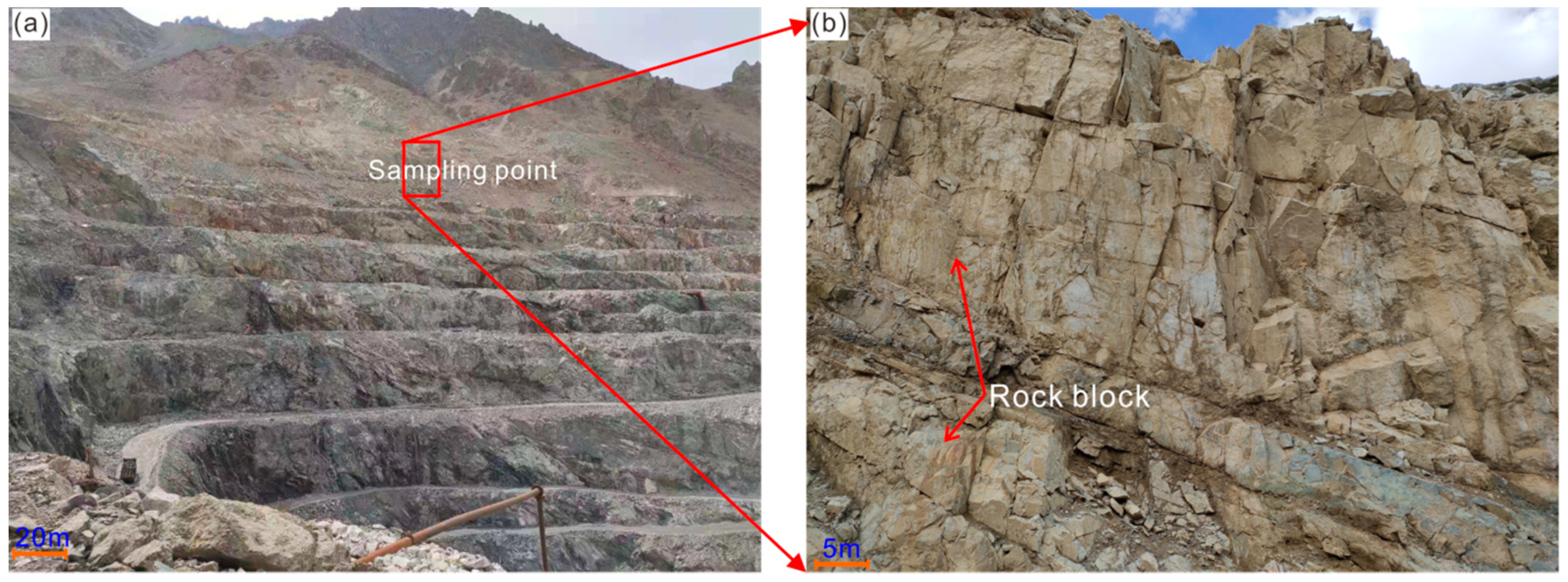
2.1. Rock Material and Sample Preparation

The studied rock material was obtained from the Hejing Beizhan open pit slope located at the Xinjiang province, in the northwest of China (Figure 1). The lithology of the rock is granite, which is distributed at the west boundary of the open pit slope, as shown in Figure 1b. The rock slope is subjected to repeated freeze and frost cycles due to climate changes. According to the climate characteristics, the mining area belongs to the continental, temperate, semi-arid climate; for the alpine, cold climate area with snow all year round, the temperature is extremely low. The monthly average temperature from January to April and from September to December is below zero, with the lowest temperature being −40 °C. The temperature rises from May to August, and the highest temperature is about 20 °C, generally about 5–15 °C. The temperature on a summer night is generally −3 to −5 °C, and the temperature difference between the day and night is relatively large. The rock cores were drilled and prepared in a cylindrical shape with a diameter (D) of 50 mm and a height (H) of 100 mm according to the ISRM’s (International Society for Rock Mechanics and Rock Engineering) suggested methods. Both ends of the samples were polished to ensure that there was an error of unevenness less than 0.05 mm, and parallelism of both ends was less than 0.1 mm.

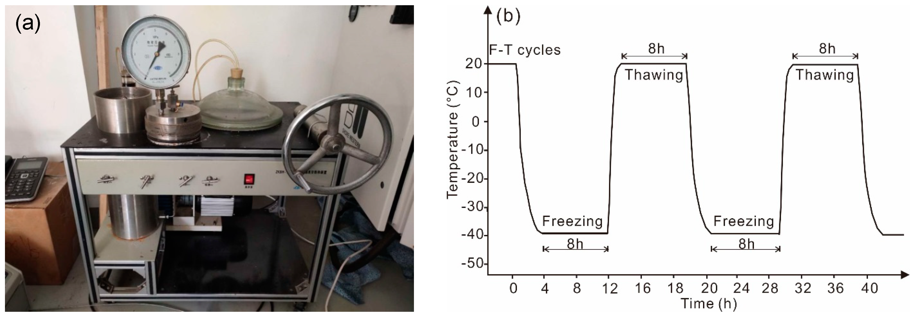
2.2. Freeze–Thaw Treatment

The samples were subjected to vacuum saturation for 24 h before the F–T treatment using a vacuum saturation apparatus (BHG300, Changji test apparatus, Tianjian, China), as shown in Figure 2a. A JS-DW-40 ultra-low temperature freezer (JS-DW-40, Ningbo, Zhejiang, China) was used to realize F–T cycles. According to the temperature changes of the open mining pit, during the F–T treatment, saturated samples were placed into the F–T apparatus and adjusted for 8 h for −40 °C, and then the samples were removed from the freezer and placed into the water at 20 °C, where they were allowed to thaw for a duration of 8 h, as shown in Figure 2b. Under freezing conditions, the rock was wrapped with cotton cloth in order to ensure the fully frozen state. Here, six groups of granite samples were treated with F–T cycles of 0 (no treatment), 20, 40, 60, 80 and 100, respectively. The basic physical and mechanical parameters of the rock are listed in

Table 1. The basic mechanical and physical parameters of the granite samples subjected to freeze–thaw (F–T) treatment.

Sample ID	L × d (mm × mm)	Mass (g)	Density (g/cm3)	Peak Strength (MPa)	Elastic Modulus (MPa)	P-Wave Velocity (m/s)	S-Wave Velocity (m/s)
G0-1	100.07 × 49.06	541.4	2.863	172.38	58.65	4302	3577
G0-2	100.01 × 49.62	540.5	2.796	182.45	60.08	4412	3456
G20-1	99.58 × 49.30	543.1	2.859	168.73	56.31	4131	3391
G20-2	100.01 × 50.21	540.2	2.729	167.24	55.46	4265	3325
G40-1	99.85 × 50.05	542.6	2.763	163.98	52.78	4012	3101
G40-2	100.12 × 49.63	544.9	2.815	158.35	53.44	4000	3210
G60-1	100.22 × 49.85	547.5	2.800	158.78	50.89	3906	2984
G60-2	100.06 × 49.19	544.6	2.865	155.66	49.65	3894	3015
G80-1	99.90 × 49.88	548.9	2.813	152.39	47.36	3826	2883
G80-2	100.11 × 49.76	543.5	2.793	149.23	45.23	3856	2913
G100-1	100.12 × 49.29	547.2	2.866	146.65	42.94	3690	2664
G100-2	100.08 × 49.34	546.6	2.858	142.33	43.89	3546	2703

.

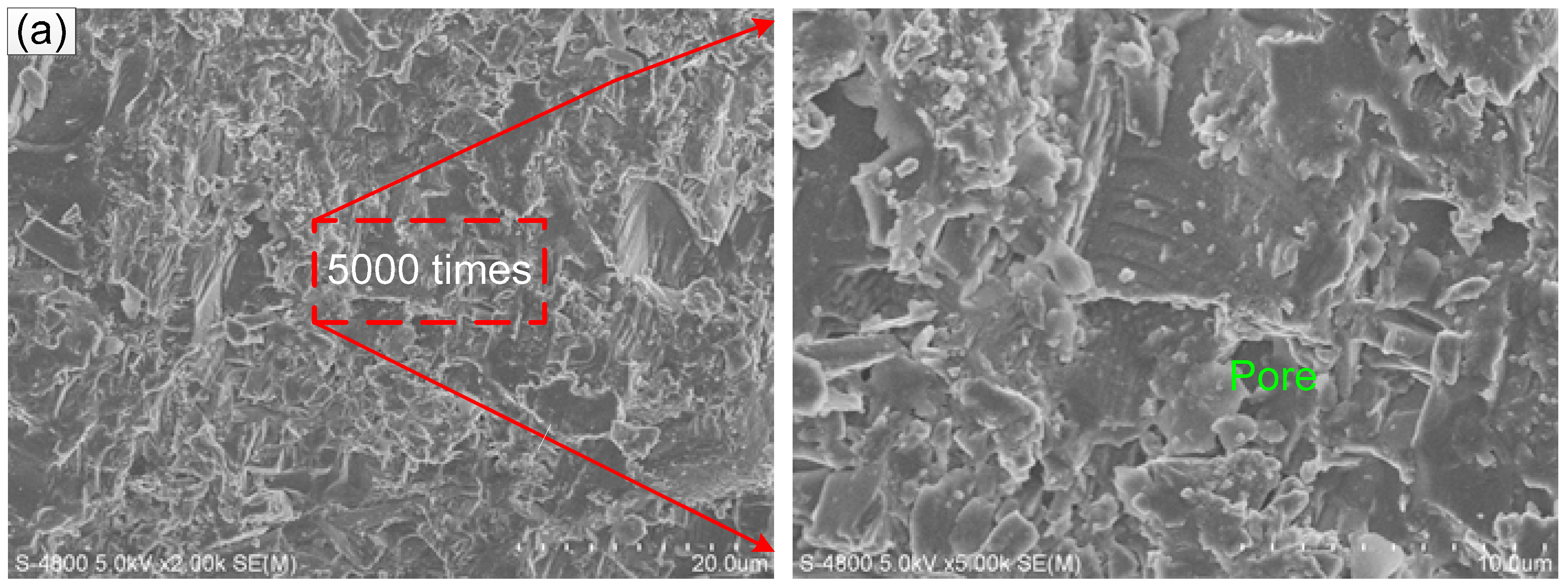
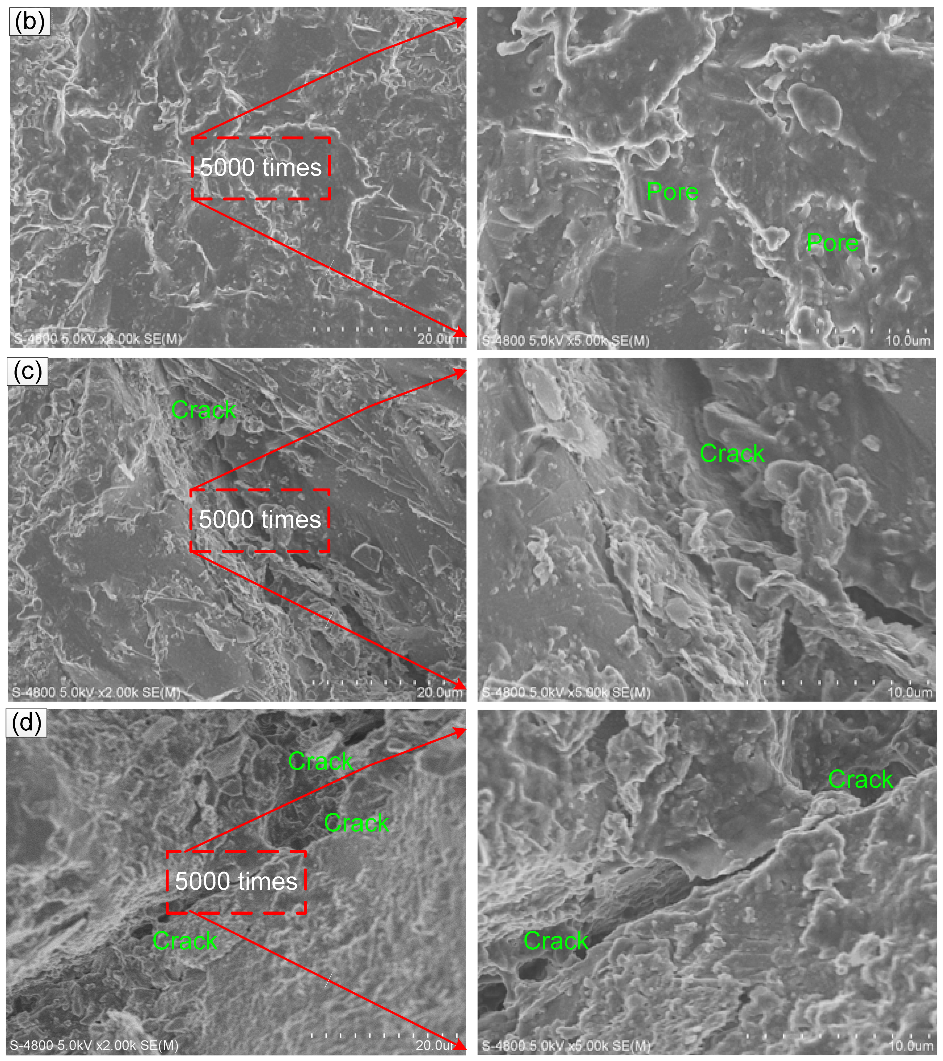
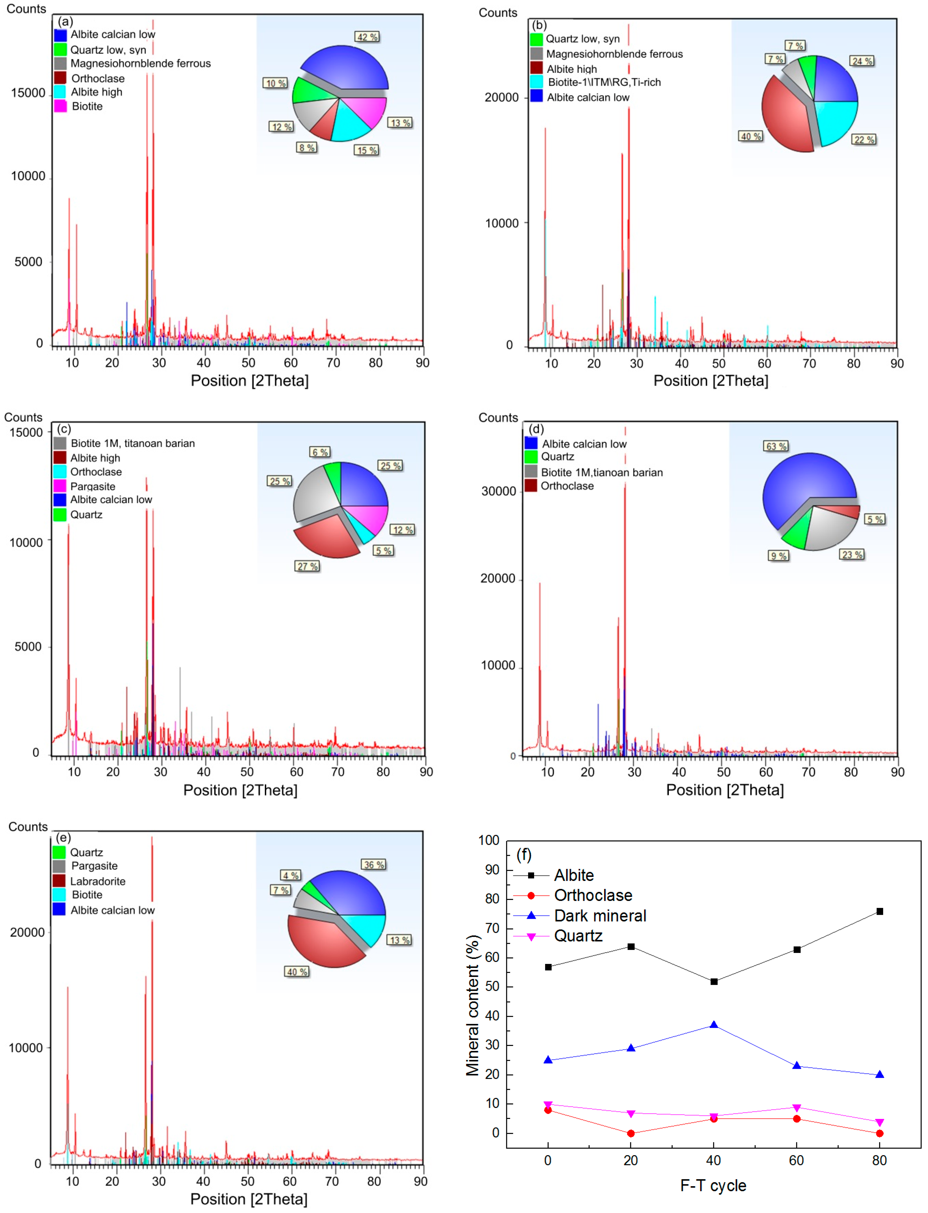
2.3. Rock Meso-Structure Identification

To describe the damage characteristics of the rock samples subjected to different F–T cycles, a Zeiss SIGMA 300 FEM-SEM testing machine (SIGMA 300/VP, Carl Zeiss AG, Jena, Germany) was used to observe the surface morphology of granite on the micrometer scale. The maximum resolution can reach 0.8 nm; the acceleration voyage is 0.02–30 kV; the maximum magnification time is 200 million times. It is equipped with 7 detectors, and 1 charge neutralizer. A powdered rock sample was used to conduct XRD testing (MXP21VAHF, MACSCIENCECO, LTD, Tokyo, Japan), in order to determine the mineral variability and mineral compositions for granite subjected to different F–T cycles.

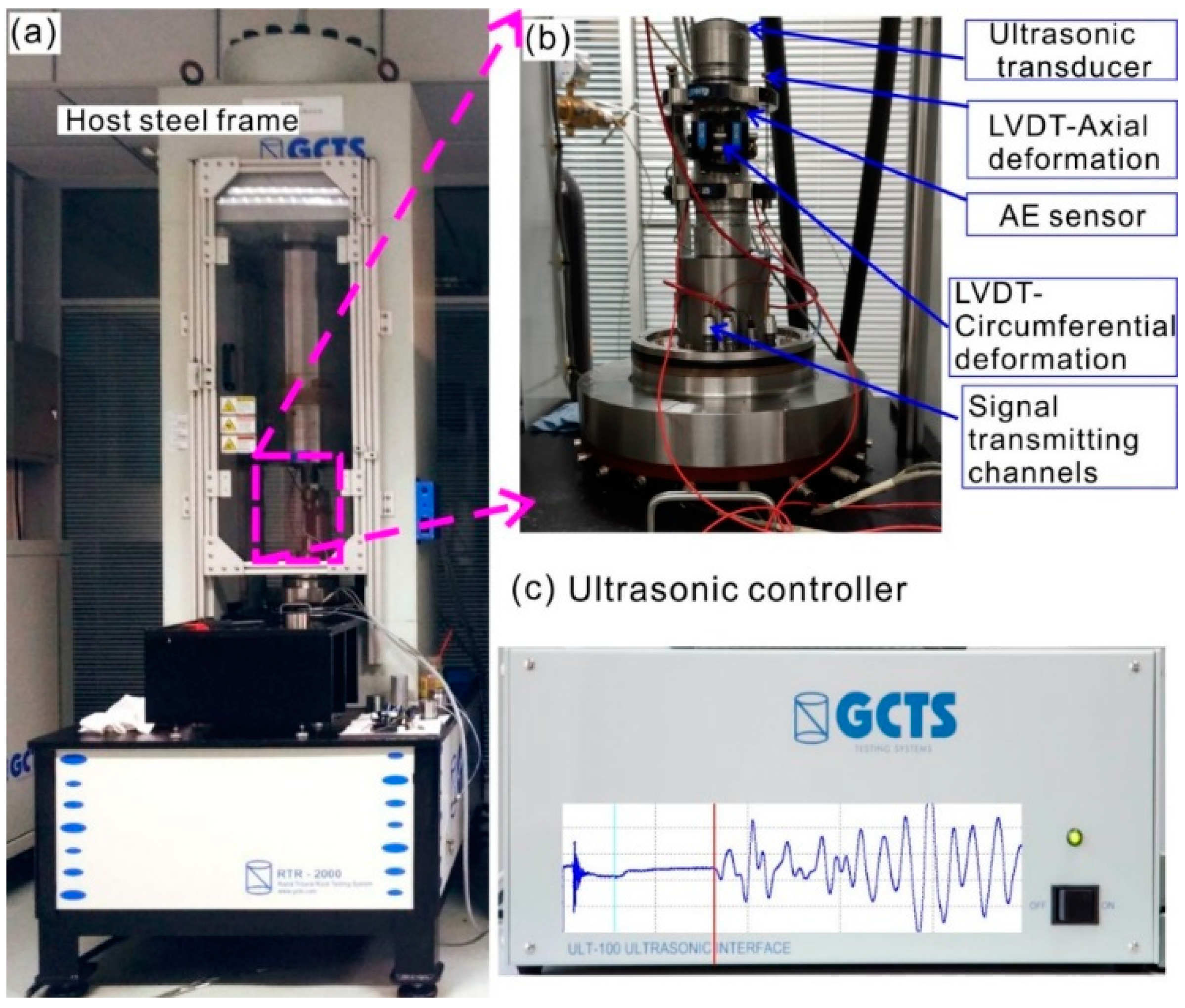
2.4. Uniaxial Compression Test

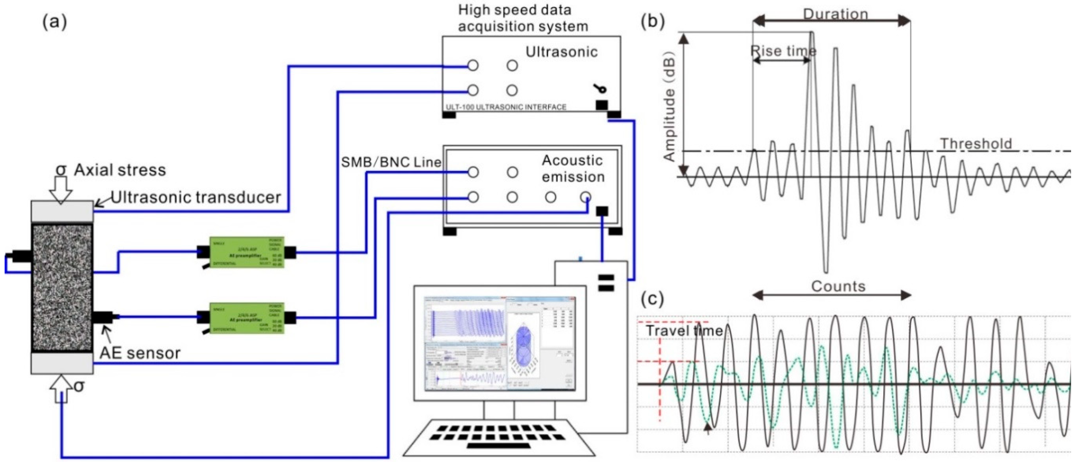
For the granite samples subjected to F–T treatment, uniaxial compression testing was conducted on a GCTS RTR 2000 rock mechanics (GCTS 2000, GCTS Testing, Arizona, Tempe, USA) with a constant loading rate of 0.06 mm/min, as shown in Figure 3. During the experiment, the lateral and axial strains were simultaneously measured by one circumferential sensor and two axial sensors (LVDTs system). A central computer was used to record strength and deformation information, including axial, axial stress, and lateral strain of the same sampling frequency. In this study, two samples were prepared for each experimental group.

2.5. AE Monitoring

During the uniaxial compression test, the AE technique was used to monitor the crack initiation, propagation and coalescence behaviors during the whole fracture process. In accordance with the AE principle, a series of AE analysis approaches, including counting the AE event rate (or cumulative numbers), counting the AE energy, examination of the amplitude distribution and investigations on the frequency of the characteristic signals, were used to reveal the effect of F–T fatigue damage on the deterioration of the granite samples. During the experiments, a PAC AE monitoring system made by Physical Acoustic Corporation Ltd. (Princeton, NJ, USA), London was used to record the AE signals. The AE monitoring system includes the AE transducers; signal acquisition; a pre-amplifier; and recording, processing and display units, as shown in Figure 4. A maximum of a 1 MSPS sampling rate with resolution of 18 bits can be realized using the PAC AE monitoring system. The sampling filter frequency is 125–750 kHz. The sampling filter frequency is 125–750 kHz. The AE system can record the AE count and energy during the deformation of the rock sample, even the entire waveforms. The AE sensor used was a miniature sensor called nano 30 with dimensions of 6 × 6 mm and a resonant frequency of 300 kHz. For the granite samples, the fracturing event was recorded using two AE sensors mounted on the sample surface (opposite positions at the top and lower), with a sample interval set to 50 μs, a threshold of 40 dB and a frequency of 102–104 Hz.

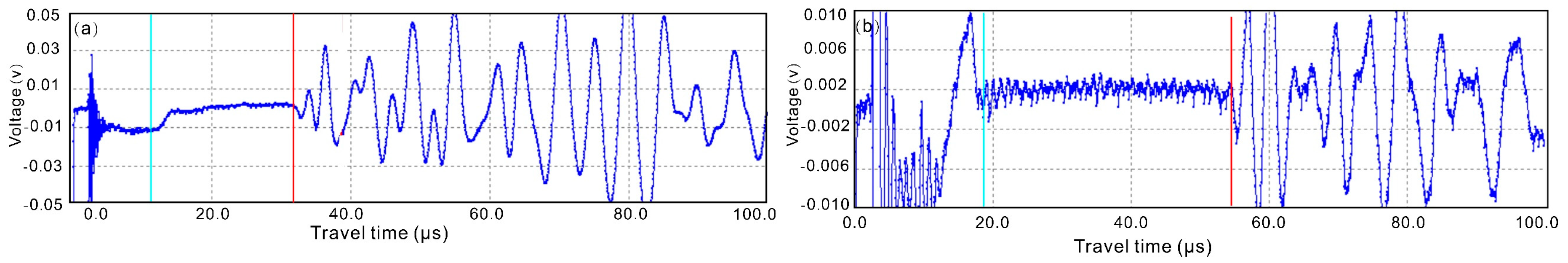
2.6. Real-Time Ultrasonic Detection

During the experiment, the P-wave and S-wave velocity between the transducers at the receiving end and the transmitter end were obtained by using ultrasonic transmission technology. The scheme of in-situ ultrasonic measurements of P and S-velocities is shown in Figure 4. In the GCTS RTR-2000 rock mechanics testing system, the ultrasonic velocity measuring subsystem (ULT-100) was used to measure the velocity of P-wave and S-wave during sample deformation, as shown in Figure 3c. The system includes two analog outputs (0-10 VDC) proportional to P and S speeds, which can be easily connected to existing data acquisition or control systems. The digitally controlled pulse generator and receiver include a switch to automatically select P or S-wave transducers. The sampling rate of the ULT-100 system is 20 MHz and the resolution is 12 bits. The ULT-100 system has an 8-channel data recorder for ±10 VDC input. The P-wave and S-wave crystal frequency of the ultrasonic transducer is 1 MHz; it can withstand 200 °C and 210 MPa. When the ultrasonic transducer is placed, the top and bottom of the shale sample are coated with a honey film to eliminate cavitation and ensure sufficient contact between transmitter and receiver transducers. For the triaxial deformation test, the P and S-velocities were recorded every 30 s, and the time window for sampling each waveform was 50 microns, with 5000 points of velocity. The P-wave and S-wave in the whole experiment process were all transmitted to the computer for further processing. The propagation time of the wave was obtained from the first periodic wave, and the velocity of the wave was calculated according to the ratio of the height of the deformed sample to the propagation time.

3. Experimental Results and Analyses

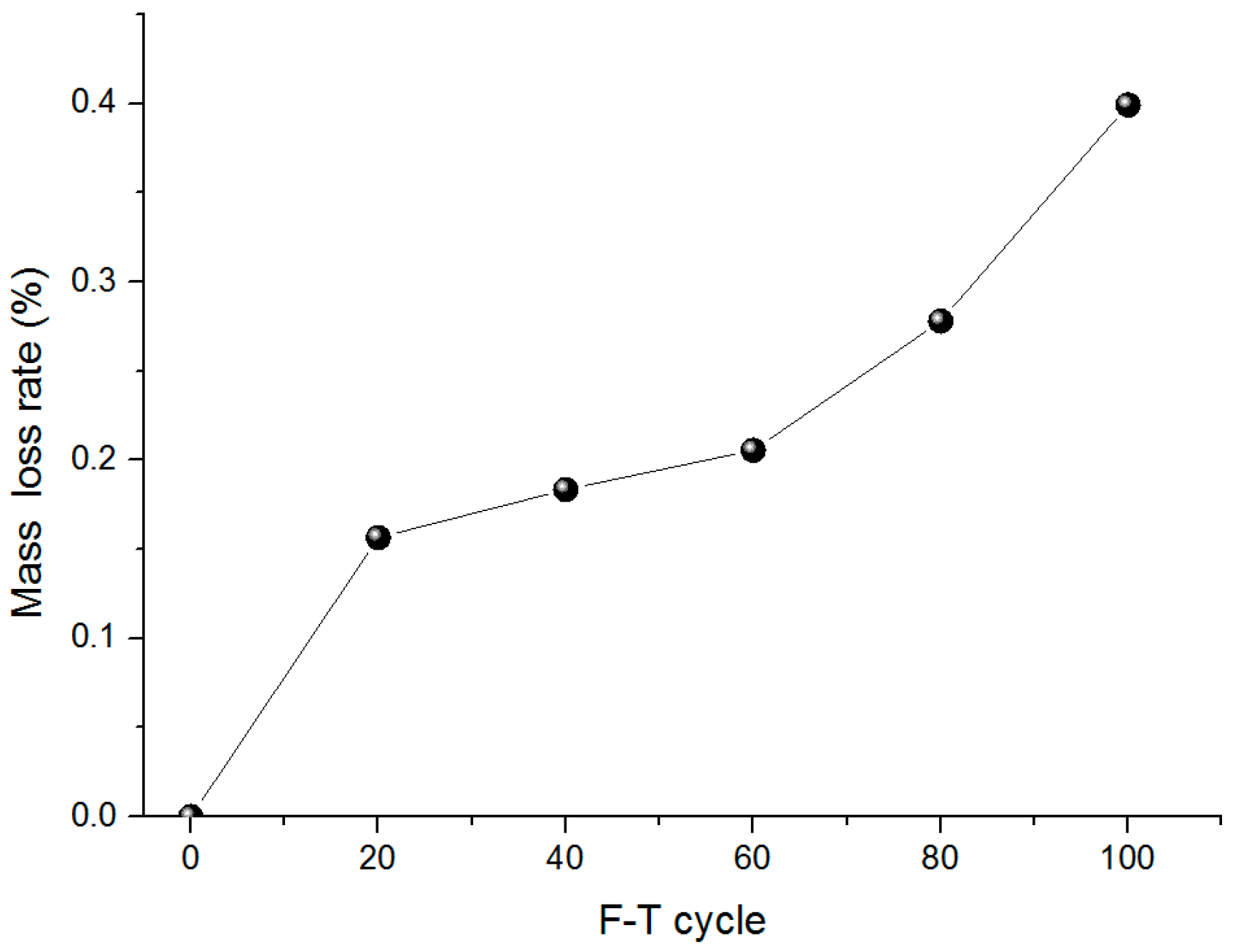
3.1. Rock Damage Subject to F–T Cycles

The analysis of the rock F–T-fatigue damage is focused on with four aspects in this work; they are the mass loss rate, P or S-wave velocity loss rate, micro-cracks in SEM pictures and the mineral variation by XRD analysis.

The mass loss rate of the granite samples at temperatures of −40 °C after different F–T cycles was calculated as the ratio of the difference of rock saturation mass to the original mass before F–T treatment. The rock mass loss rate after different F–T treatment is shown in Figure 5. It can be seen that the mass loss rate increases with the increasing number of F–T cycles, and the incremental rate becomes larger at 20 F–T cycles. This change trend is related to the rock type; for the granite studied, it is composed of medium–coarse sized minerals. The frost’s heaving pressure results from the occurrence of micro-cracks around the minerals, and the micro-crack scale increases with increasing F–T cycles. Therefore, the drop of mineral particles gradually becomes severe.

The ultrasonic velocity was measured for the rock after every F–T treatment, and then in a dry state. Figure 6 shows the velocity loss rate against F–T cycles. The P and S-wave velocity loss rates both increase with increasing F–T cycles, and it can also be found that the loss rate of the S-velocity is much larger than the P-wave. This result indicates that the frost heaving pressure is generated due to the expansion of water crystals in pores during freezing; the porosity increases accordingly, and so on, and this further results in the increases of voids and the final micro-cracks. In addition, the change of the S-wave velocity is much more sensitive than the P-wave velocity, and the S-wave velocity is much more suitable to characterize the damage of rock samples under F–T treatment.

For the rock subjected to different F–T cycles, a thin slice was cut from the cylindrical sample surface with a size of 1.0 × 1.0 cm to perform SEM imaging. Figure 7 shows that the SEM figures for the granite subjected to 0, 20, 60 and 80 F–T cycles, and every two figures with their magnifications of 500× and 5000× were used to exhibit the micro-damage characteristics. It can be seen that the pores and cracks increase with more F–T cycles. The pores begin to increase for samples subjected to 40 F–T cycles, and micro-cracks begin to occur under 60 F–T cycles. The scale of the micro-cracks and pores get to be maximal for samples subjected to 80 F–T cycles. The results indicate that even though the rock is very compacted, the moisture can still penetrate into rock defects, such as native micro-cracks and mineral boundaries. The ice lens forms and frost’s heaving stress acts at the defect surfaces, with the continuous permeation of water, and so, repeatedly, the defects gradually expand and cracking appears in the rock.

XRD was used to reveal the influence of F–T treatment on the mineral composition. Figure 8 shows the result of mineral composition for granite subjected to 0, 20, 40, 60 and 80 F–T cycles. Mineral crystal phase changes after F–T treatment and this may affect the mechanical and physical properties. Due to the high elastic modulus and hardness characteristics, and the weakest water-absorption ability of quartz, the crystal phase change of quartz is the weakest compared to the other kinds of minerals.

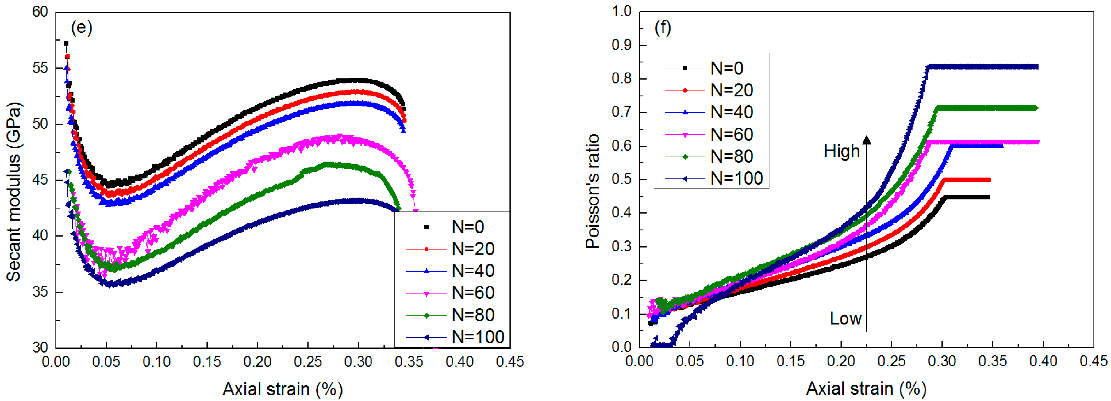
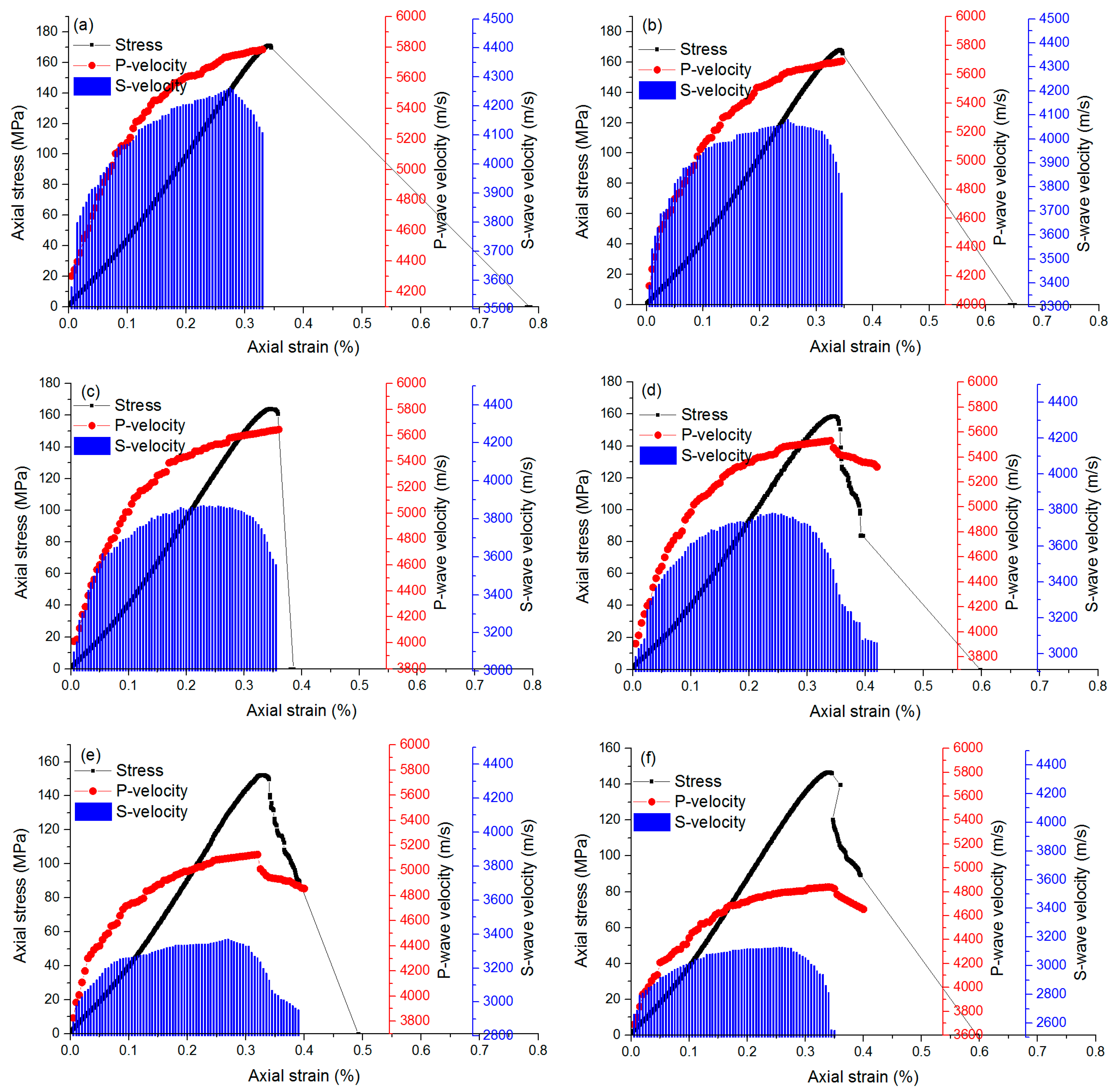
3.2. Strength and Stress–Strain Responses

With the increase of F–T damage and further expansion of micro-cracks induced by frost’s heaving stress, the internal rock structure suffers from deterioration, and this would affect the strength and deformation characteristics. Figure 9 shows the strength and the complete stress strain curves for the samples subjected to 0, 20, 40, 60, 80 and 100 F–T cycles. From the morphology of stress–strain curves, it can be seen that sudden brittle failure occurs for the samples subjected to 0, 20 and 40 F–T cycles; however, for the samples experiencing 60, 80 and 100 F–T cycles, it was not a sudden failure for these samples, and rock strength gradually decreases after the peak stress. The volumetric stress strain curve reflects well, the failure phenomenon. The sample volumetric expansion is much larger for the samples subjected to 60, 80 and 100 F–T cycles than those subjected to 0, 20 and 40 cycles. From Figure 9b, it can be seen that the final volumetric strains at the failure points are −0.442%, −0.858%, −0.933%, −5.732%, −5.533% and −5.864%, respectively. After F–T treatment, the sample plasticity increased due to the generation of pores and micro-cracks inside the rock sample. The peak stress presents a linear decreasing trend as the number of F–T cycle increases; and the elastic modulus also gradually decreases with an increasing number of F–T cycles, as plotted in Figure 9c,d. During the whole deformation process, the variation of two elastic parameters of secant modulus and Poisson’s ratio was also analyzed here. The secant modulus is defined as the axial stress to axial strain at each adjacent data, the Poisson’ ratio is defined as the lateral strain to axial strain at each data point. Evolution of the two elastic parameters with sample deformation is shown in Figure 8e,f. It can be seen the secant modulus decreases and Poisson’ ratio increases with the increase of F–T treatment.

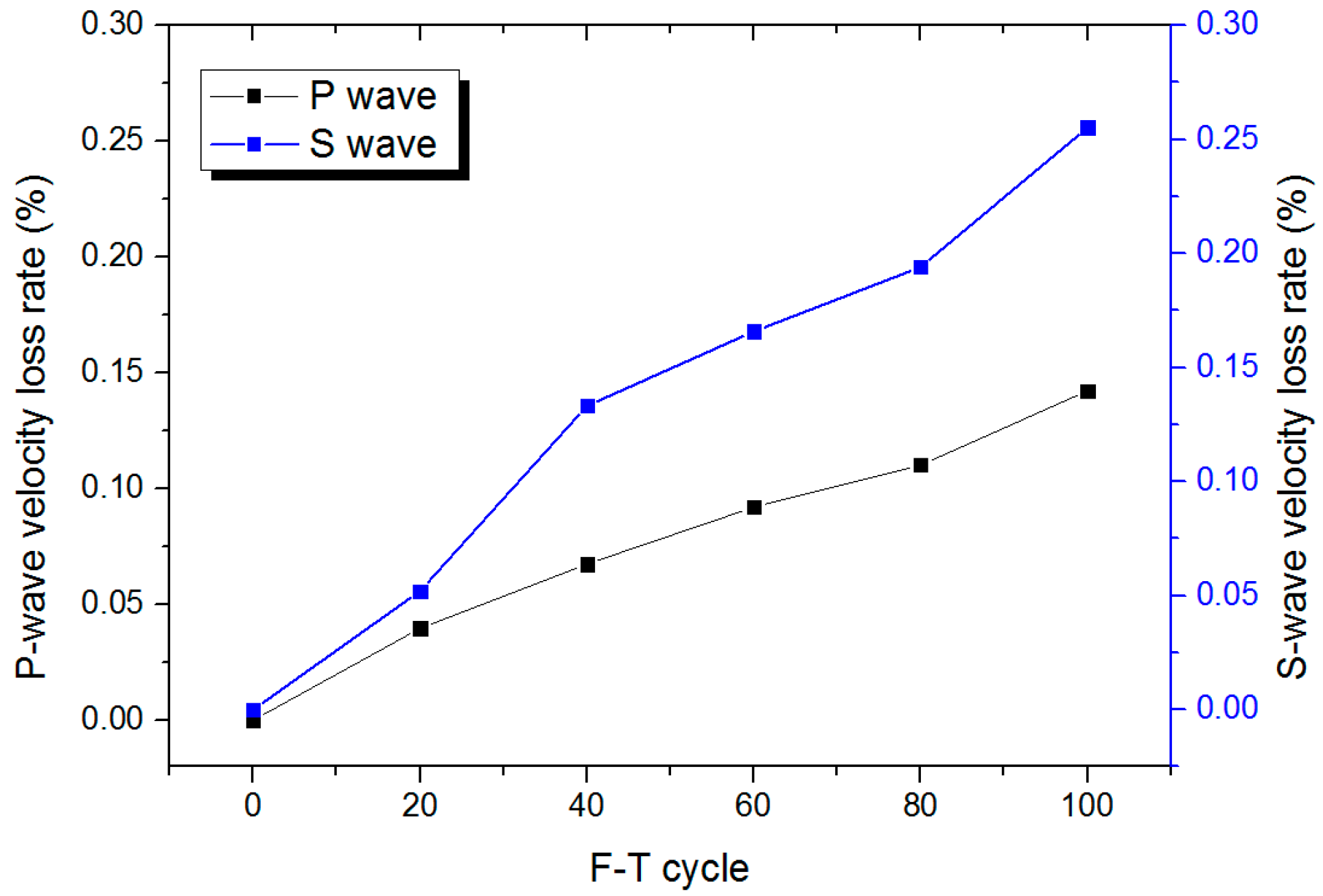
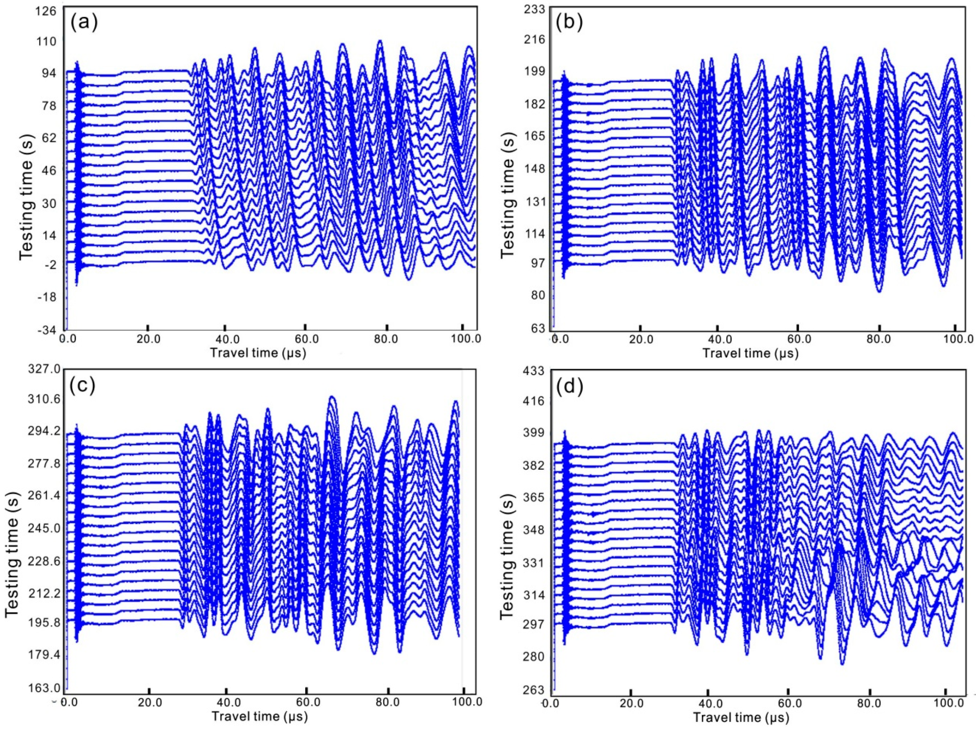
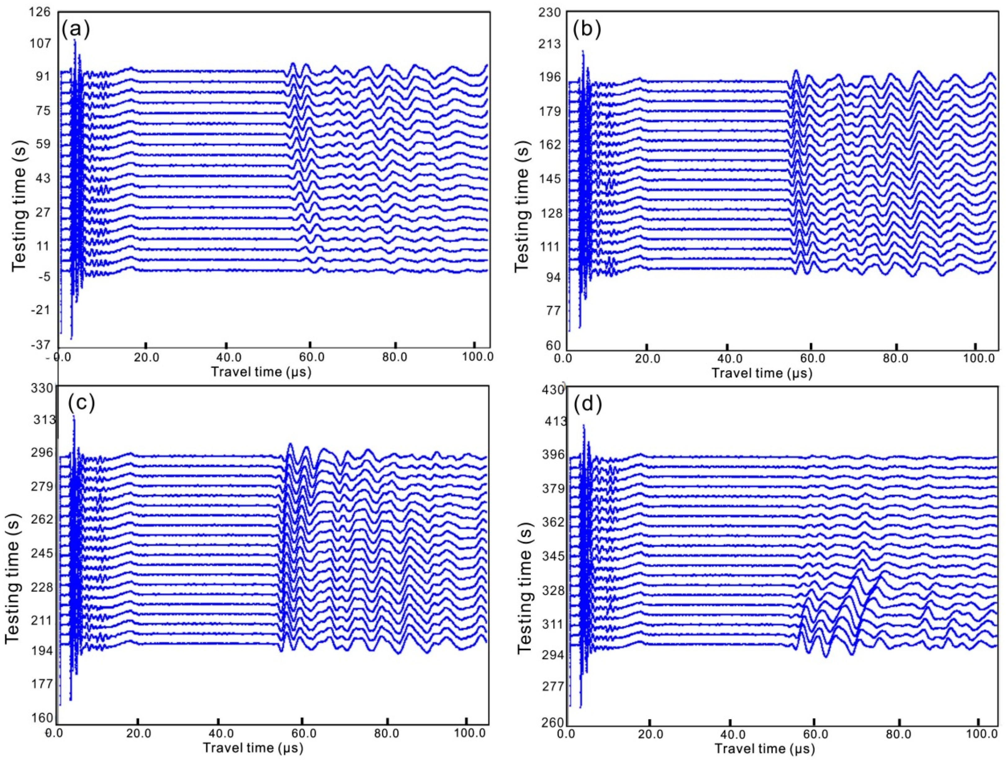
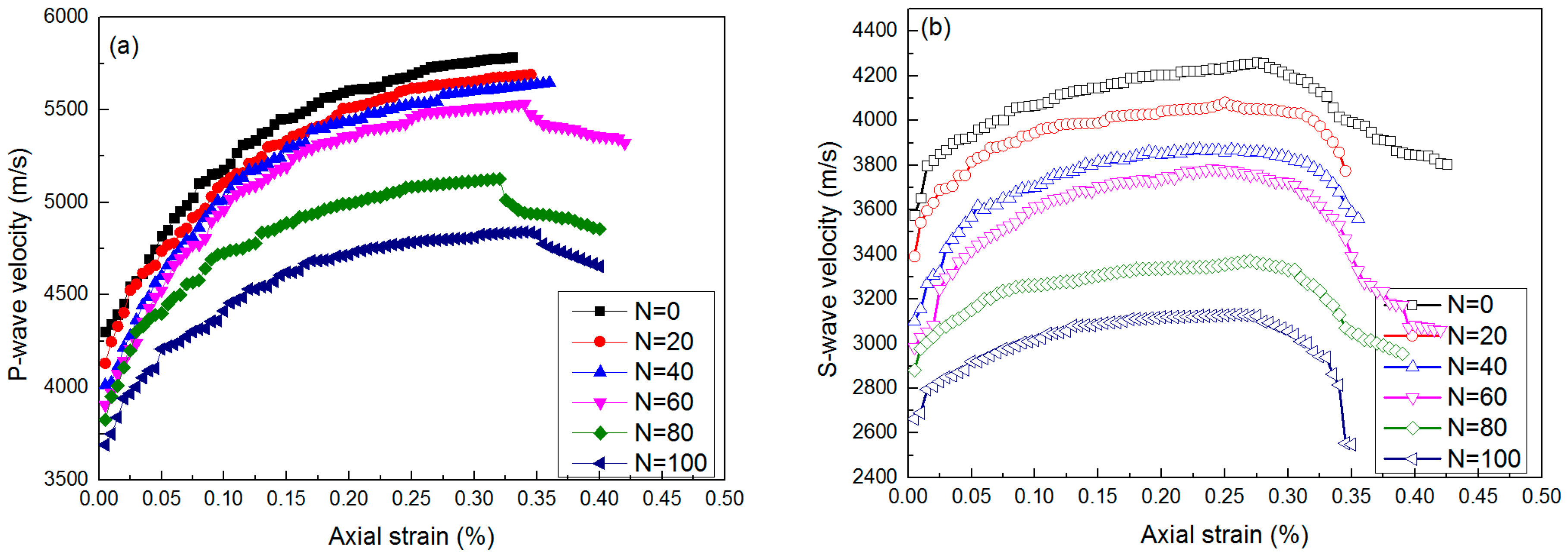
3.3. Real-Time Ultrasonic Properties of Rock

Taking a granite sample subjected to 100 F–T cycles as an example, a series of typical, first cycle P-waveforms and S-waveforms can be obtained using the ULT-100 ultrasonic subsystem, as shown in Figure 10 and Figure 11. The first cycle wave (as shown in Figure 12), because of its stability and renewable characterization under the same contact conditions and the same transducer, was used to determine the travel time. Using that method, we obtained all the P and S-wave velocities for the samples at any stress level.

Figure 13 plots the relationship between the P and S-velocities and axial strain, which are affected by the initial F–T fatigue damage in the samples. It can be seen that the P-wave velocity increases with sample deformation until failure for samples subjected to 0, 20 and 40 F–T cycles; however, it first increases and then decreases, and decreasing occurs after the peak stress. The changes of P-wave velocity reflect the failure mechanism of the rock samples; the results are consistent with the pattern of stress strain curves. For samples subjected to high F–T degradation, the post-peak curve gradually drops to zero, indicating that the failure blocks slide along the fracture surface. This result indicates the increase of ultrasonic travel time when the wave goes through the blocks, and the velocity decreases accordingly. The change trend of S-wave velocity shows, first, an increasing, and then, a decreasing trend. The velocity decreasing point may be related to the crack coalescence behaviors. Wang and Li [21] found that the stress at the decreasing point is roughly equal to the crack damage stress, and similar conclusions can be drawn for the granite samples experiencing F–T cycles. The ultrasonic velocity carries the fracture information during sample fracturing, and the rock fracture is strongly affected by its internal meso-structures. Therefore, the P and S-velocities are both affected by the F–T deterioration. Figure 14 plots the P and S-wave velocities for the samples subjected to different F–T cycles. Both P and S-wave velocity decreases with increasing F–T cycles, which are affected by the rock meso-structures; the energy of the ultrasonic wave decreases due to the scattering on pores or micro-cracks, which prolongs the time duration of the wave passing through the samples. In addition, it can be seen that the P-wave velocity is larger than the S-velocity, and the S-wave is much more sensitive during sample deformation; this result has been proven in the above section.

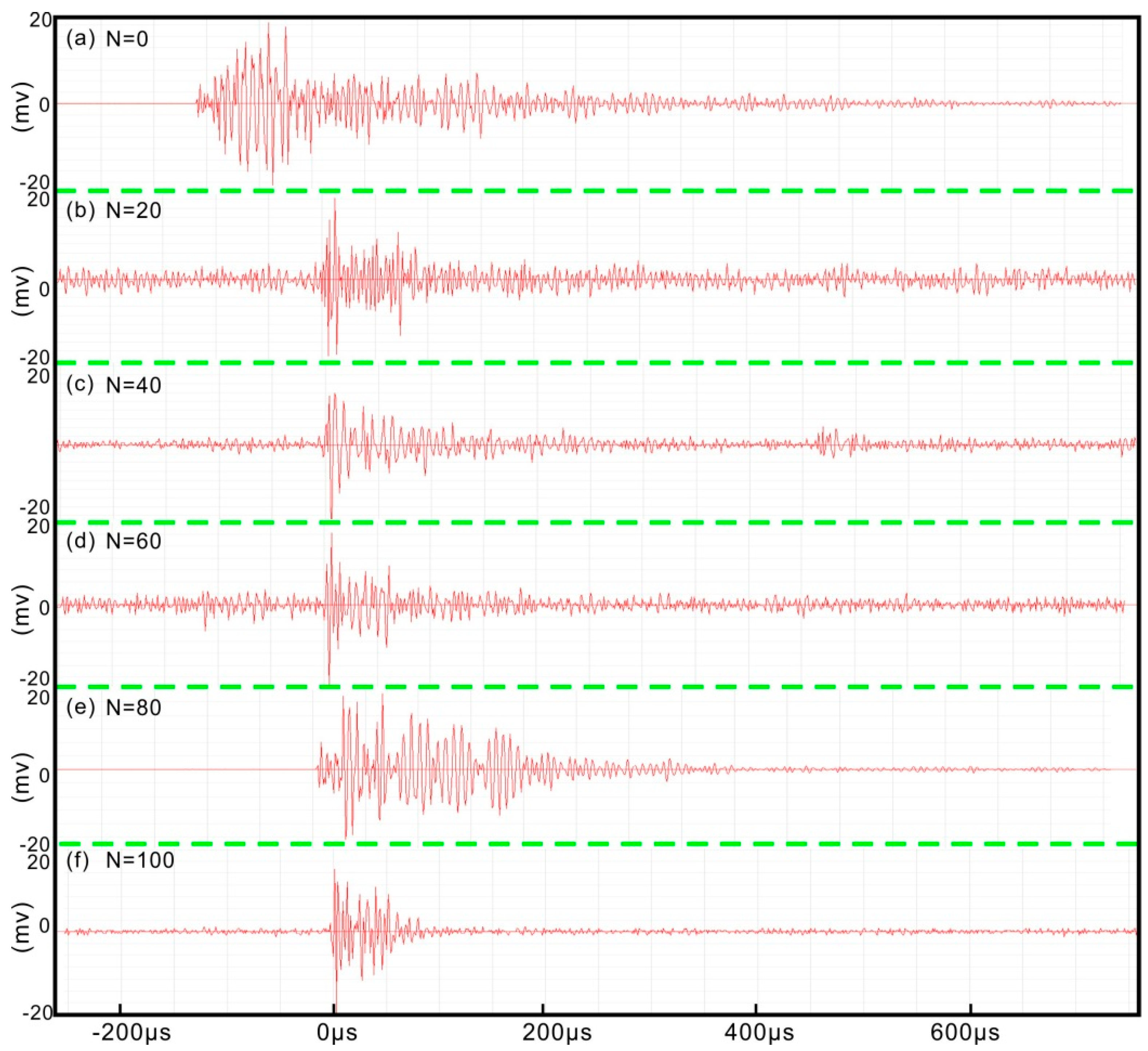
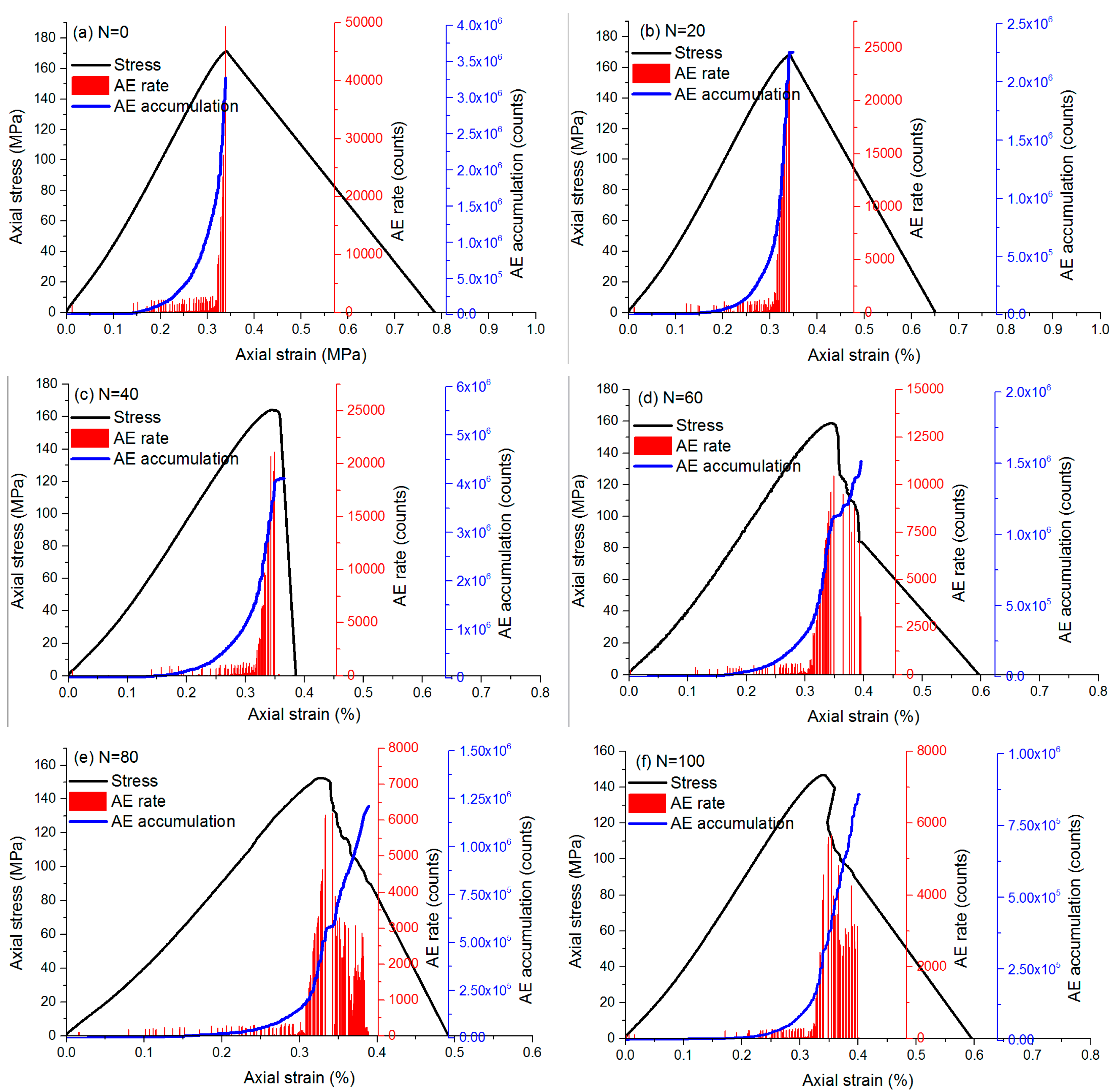
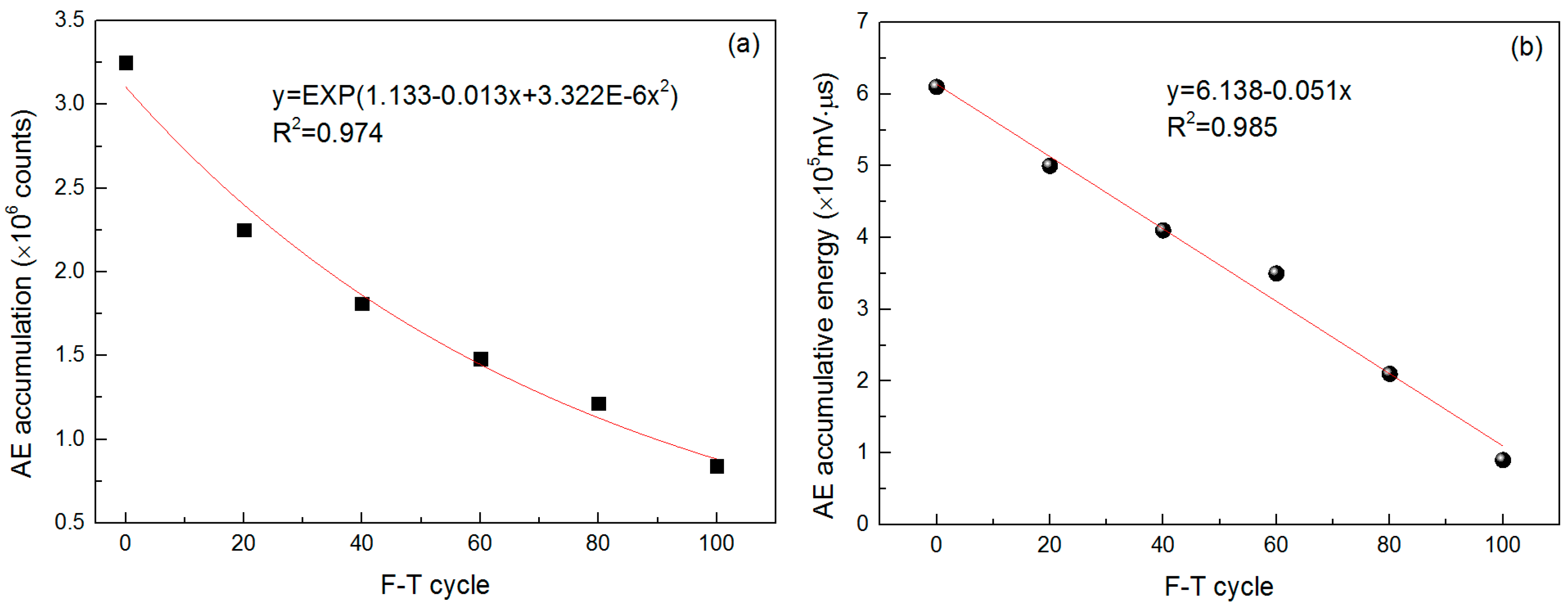
3.4. AE Count Characteristics

The AE count curves reflect the progressive failure characteristics of granite samples; the crack initiation, propagation and coalescence are related to the change of AE count. During AE monitoring, the waveform of every AE event can be obtained; the parameters of AE counts and energy release can be calculated from the waveforms. Typical AE waveforms for the samples at their failure points are shown in Figure 15.

As shown in Figure 16, a silent period exists before crack initiation, and once a crack initiates, the crack propagates until sample failure. The AE count curve presents different patterns which are influenced by the failure characteristics. And this is attributed to the difference of material structure after the F–T treatment. The AE counts suddenly increased at the failure point for the samples experiencing 0, 20 and 40 F–T cycles. However, the AE counts were also recorded at the post-peak stages for the samples experiencing 60, 80 and 100 F–T cycles. Plenty of AE signals are generated at the post-peak stage and fracture of rock continuously proceeds. The accumulative AE counts shows an increasing fluctuation trend at the post-peak stages, which reflects the discontinuous deformation characteristics.

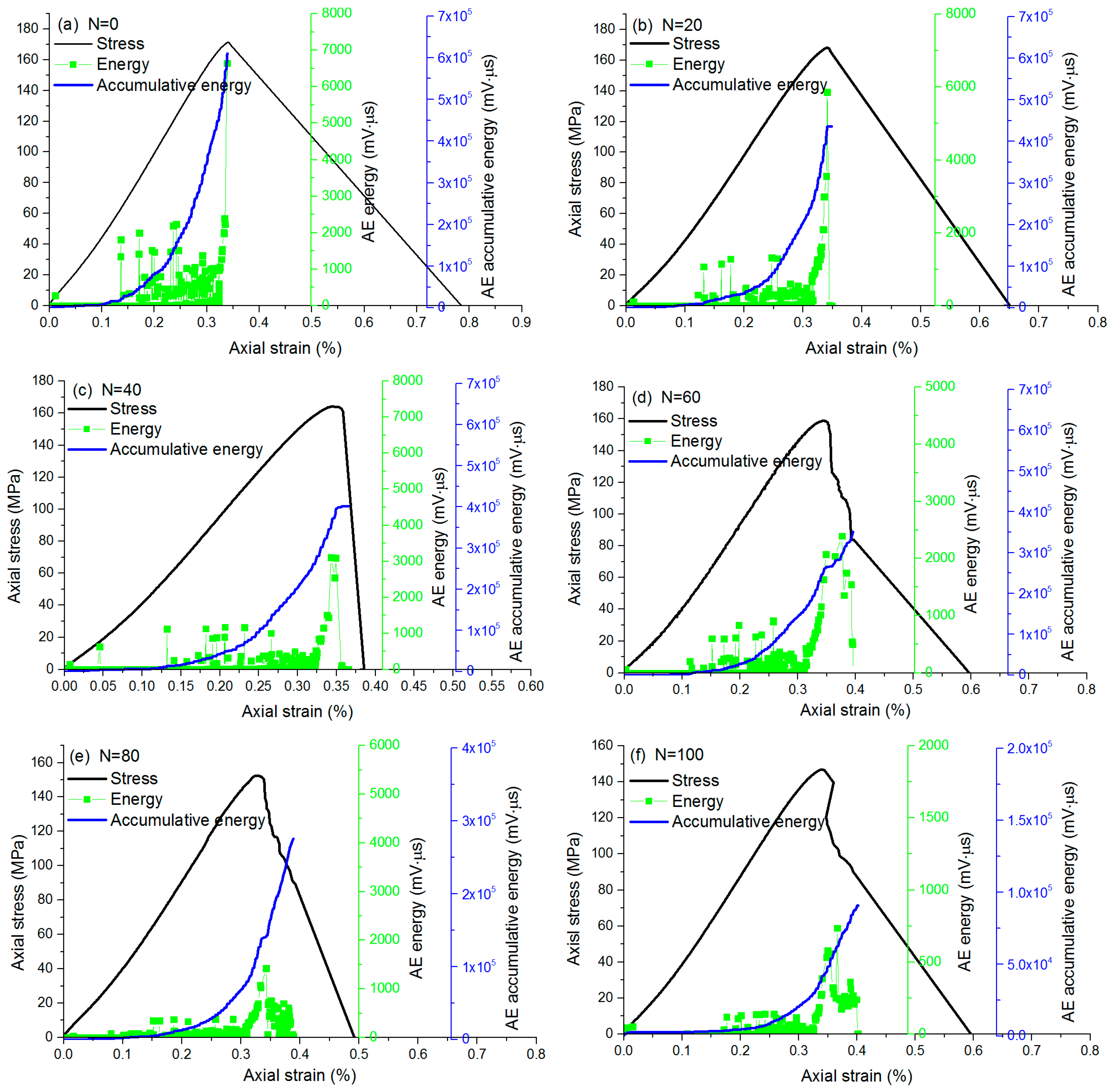
3.5. AE Energy Characteristics

Apart from the AE count, the AE energy is also an effective parameter to represent the fracture characteristics of rock. The AE energy monitored by the AE sensor is a kind of absolute energy, it is generally defined as a measured area under the rectified signal envelope. It is a multiplication of the amplitude by the time span of the event [22]. The mean monitoring data of the two sensors was used in this work, and the unit of the energy is mv·μs. Because the AE energy is sensitive to the amplitude, as well as the duration, and it is less dependent on the operating frequencies and voltage threshold, this parameter is usually preferred for interpreting the magnitude of the source event over AE counts [23], and it can better reflect the crack initiation, propagation and coalescence. The effect of F–T damage on the AE energy evolution of granite with different F–T treatment is shown in Figure 17. Under a lower stress level, the energy release is relatively lesser, and it increases continuously and quickly until failure of the granite samples. Lower energy release indicates a balance period for the rock sample. With the formation of micro-cracks during sample deformation, high AE energy release was recorded, which was recorded by the skipping of the accumulated energy curve. Near the peak stress point, the growth and coalescence of cracks leads to the rapid increment of AE energy release; and AE energy release can still be recorded at the post-peak stage due to the sliding of fractured rock blocks along the fracture surface.

For the granite samples, the relationships between the accumulative AE counts, accumulative AE energy and F–T cycles are plotted in Figure 18. It was found that the accumulative AE counts and energy decreased with increasing F–T cycles. The cyclic F–T effect aggravates the damage of the rock samples by means including the generation of micro-cracks, dissolution and variation of rock minerals, decrement of cementation degree, etc. The energy used to drive the crack propagation becomes smaller with the increase of F–T cycles, and the AE counts and the energy released during crack propagation and coalescence becomes smaller accordingly. In order to reveal the relationships between AE accumulative count, AE accumulative energy and F–T cycle number, power, linear, polynomial, exponential and logarithmic regression fitting methods were executed, and the regression equations that had the largest correlation coefficient were finally determined. The fitting results show that the relationship between the AE accumulation count, AE accumulation energy, and F–T cycle number obey exponential and linear relationships, with correlation coefficients of 0.974 and 0.985, respectively.

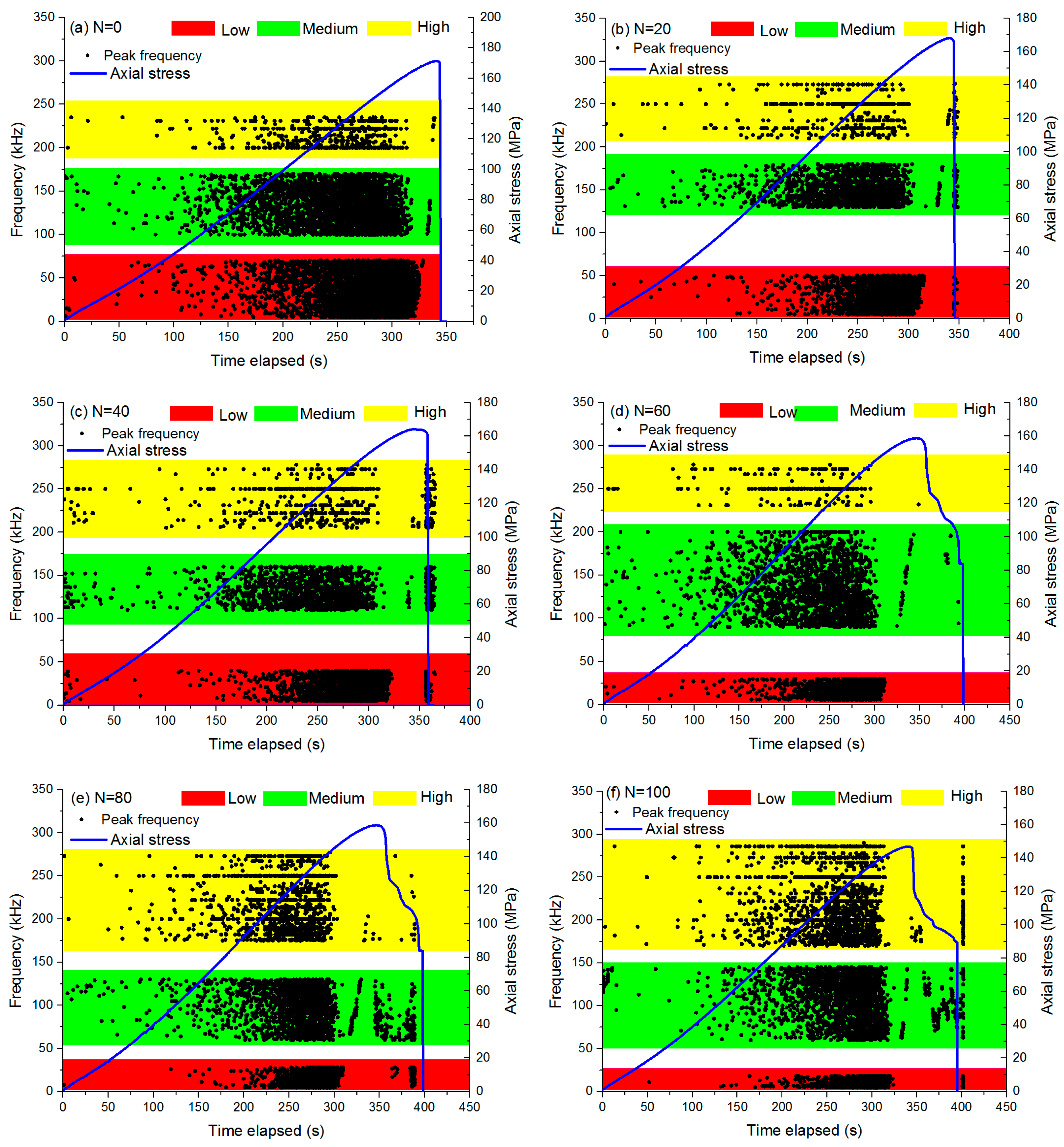
3.6. AE Spectrum Frequency Characteristics

The AE signals consist of a variety of frequency components, and the waveform frequency and amplitude are different for different AE sources [24,25,26]. The waveform characterization can reflect the crack type, number and scale; therefore, the spectrum (frequency) information can reflect well, the fracture process of the rock. Existing research results have shown that the AE main frequency characteristics can better reflect the micro-fracturing of rock, and they are much more sensitive to the AE counts [24]. Different damage modes have been found to release AE signals with different frequency characteristics. Investigation of the frequency characteristics of emission events, on which our attention will be focused in this section, could be significant and promising as a means of characterizing the effects of the F–T cycle on the fracturing process. By using the fast Fourier transform (FFT), the extracted discrete time domain signal can be transferred to a continuous frequency domain signal; the main frequency distribution during the whole fracturing process is shown in Figure 19. Low frequency, median frequency and high frequency AE signals could be observed during the whole sample deformation; however, the band widths were different for the different samples. The frequency spectrum band distribution is listed in

Table 2. Frequency spectrum characteristics of granite during the fracture process, subjected to different F–T cycles.

F–T Cycle (N)	Low Frequency (kHz)	Median Frequency (kHz)	High Frequency (kHz)
0	[0, 75]	[105, 175]	[195, 235]
20	[0, 55]	[125, 178]	[210, 275]
40	[0, 45]	[110, 160]	[205, 280]
60	[0, 30]	[90, 200]	[235, 275]
80	[0, 25]	[65, 130]	[175, 275]
100	[0, 20]	[65, 145]	[170, 290]

.

The frequency band for the samples subjected to different F–T cycles is listed in Table 2. It can be seen that the width of the low frequency band decreases and the width of the high frequency band increases with increasing F–T cycles. The AE studies on the fracture process of rock material have shown the stress waves in the form of acoustic emission (AE) signals can give insights into the process of energy dissipation and emission in response to the crack initiation and propagation. There is an inverse relationship between the AE frequency and the crack size. Generally, large-scale cracks correspond to low frequency signals, and small-scale cracks correspond to high frequency signals. The AE frequency band distribution indicates the mesoscopic fracturing mechanism of rock. For a sample without F–T treatment, strong brittle fracturing occurs and the crack propagation and the coalescence pattern is relatively obvious. Plenty of tensile micro-cracks form at the failure moment; therefore, the AE frequency is accordingly high. However, for a sample subjected to high F–T treatment, many micro-cracks from pores are already generated by the frost’s heaving force, and the rock structure suffers series damage before loading; for this kind of sample, relatively large-scale crack form and its number is smaller at the failure point. From the results of AE activity analysis by counting the event rate (or the cumulative numbers) and observing AE energy (or the cumulative energy), the AE frequency results can also be proven. At the post-peak stage, shear sliding of rock blocks indicate the formation of relatively large cracks.

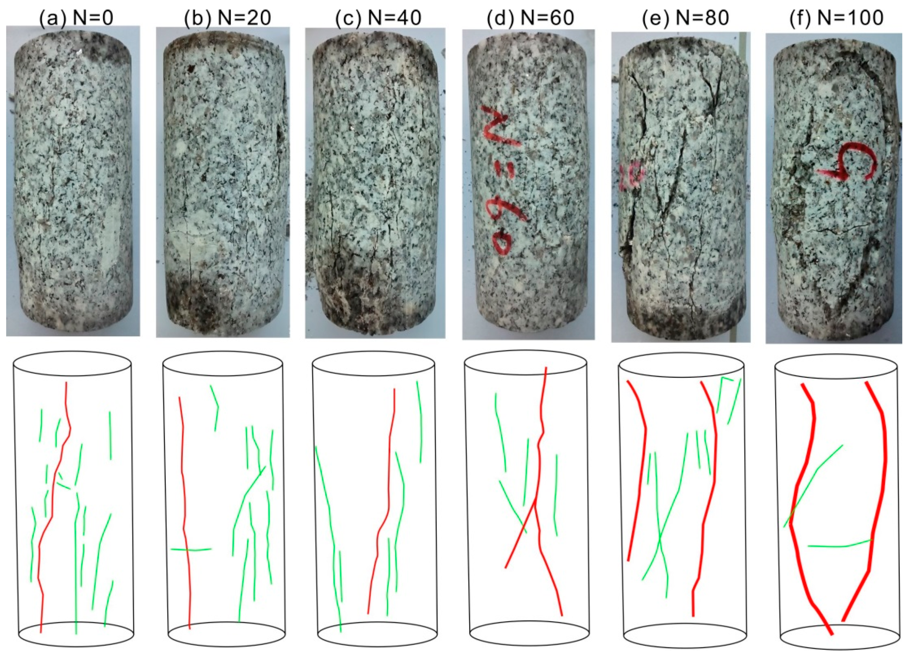
3.7. Macroscopic Failure Morphology Analysis

After the uniaxial deformation test, the fracture morphologies of the granite samples were observed by the naked eye, as shown in Figure 20. For the samples subjected to different F–T cycles, the failure mode is impacted by the F–T treatment. For samples subjected to 0, 20, 40 or 60 F–T cycles, tensile spitting failure plays a dominant role; however, for samples subjected to 80 or 100 F–T cycles, shear failure plays a dominant role. For the sample with F–T treatment, plenty of small-scale cracks can be observed; for the sample subjected to relatively high F–T treatment, it can be seen that large-scale cracks occur. The failure morphology indicates that number of small-scale cracks decreases, and large-scale cracks increase in number. This result is in consistent with the AE spectrum frequency analysis; a small-scale crack usually corresponds to high frequency signal, and a large-scale crack corresponds to a low frequency signal. The low frequency band’s signals decrease, indicating the occurrence of large shear cracks. This can be seen from the crack pattern sketch map, showing large-scale shear cracks generated in the samples subjected to 80 or 100 F–T cycles. The occurrence of shear cracks implies the increase of rock plasticity after repeated F–T treatment.

4. Discussions

Although many attempts have been made to investigate the impacts of the freeze–thaw cycle on rock’s mechanical properties, most of the studies focused on the macroscopic fracture behaviors by analyzing the stress–strain responses and final failure morphologies of rock. The investigations of the acoustic properties of rock subjected to different F–T cycles are not well studied. In situ AE monitoring and ultrasonic detection have been conducted on granite samples with different F–T treatments; the strength, deformation and fracturing behaviors were systematically investigated by the analysis of AE counts, AE energy, frequency spectrum characteristics and failure morphology analysis. The P and S-velocities during sample deformation were first recorded for the F–T rocks. The change of ultrasonic velocity indirectly reflects the F–T fatigue damage on rock meso-structures.

For rock having a high damage degree caused by F–T cycles, many pores and micro-cracks exist inside the rock. The meso-structure is worsened by the defects; therefore, the associated energy release velocity is relatively low, and the AE counts/energy (or accumulative number) are lower than rock without or having low F–T damage. The AE event parameter’s analysis revealed the progressive failure process of rock, and the AE curve pattern was impacted by the F–T cycles. For rock subjected to high F–T treatment, the AE signals at the post-peak stage are more than the samples with low F–T cycles; in addition, the accumulated AE counts/energy curves present a step-increasing trend at the post-peak stages for the sample experiencing high F–T treatment. The testing results further revealed the frequency-spectral characteristics of rock: the crack number and scale decrease under compression with increasing F–T cycles, and the low frequency band width becomes smaller. The non-linear mechanical behaviors and physical mechanisms of rock deformation can be investigated essentially from the perspective of energy evolution. Apart from the AE energy monitoring by AE sensors, the macroscopic failure morphology description was also conducted to reveal the impact of F–T treatment on the failure mechanism. It was found that the rock plasticity increased and brittleness decreased as number of F–T cycles increased. Failure mode is affacted by F–T action. The failure mode changes from tensile mode to shear mode, and the crack scale and density changes for samples subjected to different F–T cycles. The testing result shows that the crack scale and density in the failed samples are the same as the AE spectrum frequency analysis. Plenty of small-scale cracks were stimulated for the samples subjected to low F–T treatment, and small amount of small-scale cracks were generated for the samples subjected to high F–T treatment.

5. Conclusions

This study focused on investigating the effects of freeze–thaw cycles on the geomechanical and acoustic properties of granite samples. The samples were treated with artificial F–T cycles to mimic the field environments. The experimental results reveal the effects of F–T fatigue damage on the meso-damage, strength, deformation, ultrasonic velocities, AE patterns and energy transformation characteristics. The following conclusions can be drawn from this study:

(1) Frost’s heaving stress during F–T treatment causes the meso-structural changes of rock, and the rock structure deterioration further impacts the mechanical and acoustic properties of granite, such as mineral composition, surface morphology, mass loss rate, velocities, UCS, AE pattern and failure mode.

(2) The AE counts/energy curves present a different pattern for samples subjected to different F–T cycles. The number of fracturing events decreases with increasing F–T cycles. The accumulated AE counts and accumulated AE energy show a decreasing trend as the number of F–T cycles increases. Frequency spectrum analysis reveals the stimulated crack scale, and the width of the low frequency band decreases and high frequency band increases close to sample failure. This result indicates the increment of large-scale cracks and the decrement of small scaled cracks affected by F–T action.

(3) Macroscopic failure morphology description further indicates the failure mechanism impacted by F–T treatment. For a sample subjected to high F–T cycle, shear failure mode plays a dominant role and the crack scale is relatively large with low crack density; the energy used to drive the propagation of crack is relatively less.

(4) Good agreement has been found from the AE parameter analysis, spectrum frequency analysis and failure pattern description. The energy release gradually decreases with increasing F–T cycles, and the crack scale generated during sample deformation decreases. It is suggested that the F–T fatigue damage has influences over rock energy storage and release characteristics, and the instability of rock engineering in cold regions.

References

1. Halsey, D.P.; Mitchell, D.J.; Dews, S.J. Influence of climatically induced cycles in physical weathering. Q. J. Eng. Geol. Hydrogeol. 1998, 31, 359–367. [Google Scholar] [CrossRef]
2. Matsuoka, N. Microgelivation versus macrogelivation: Towards bridging the gap between laboratory and field frost weathering. Permafr. Periglac. Process. 2001, 12, 299–313. [Google Scholar] [CrossRef]
3. Yamabe, T.; Neaupane, K.M. Determination of some thermo-mechanical properties of Sirahama sandstone under subzero temperature condition. Int. J. Rock Mech. Min. Sci. 2001, 38, 1029–1034. [Google Scholar] [CrossRef]
4. Takarli, M.; Prince, W.; Siddique, R. Damage in granite under heating/cooling cycles and water freeze-thaw condition. Int. J. Rock Mech. Min. Sci. 2008, 45, 1164–1175. [Google Scholar] [CrossRef]
5. Tan, X.J.; Chen, W.Z.; Yang, J.P.; Cao, J.J. Laboratory investigations on the mechanical properties degradation of granite under freeze-thaw cycles. Cold Reg. Sci. Technol. 2011, 68, 130–138. [Google Scholar] [CrossRef]
6. Argandona, R.V.G.; Rey, A.R.; Celorio, C.; Del Río, L.S.; Calleja, L.; Llavona, J. Characterization by computed X-ray tomography of the evolution of the pore structure of a dolomite rock during freeze–thaw cyclic tests. Phys. Chem. Earth Part A Soild Earth Geod. 1999, 24, 633–637. [Google Scholar] [CrossRef]
7. Bost, M.; Pouya, A. Stress generated by the freeze–thaw process in open cracks of rock walls: Empirical model for tight limestone. Bull. Eng. Geol. Environ. 2017, 76, 1491–1505. [Google Scholar] [CrossRef]
8. Seto, M. Freeze–thaw cycles on rock surfaces below the timberline in a montane zone: Field measurements in Kobugahara, Northern Ashio Mountains, Central Japan. Catena 2010, 82, 218–226. [Google Scholar] [CrossRef]
9. Nicholson, D.T.; Nicholson, F.H. Physical deterioration of sedimentary rocks subjected to experimental freeze–thaw weathering. Earth Surf. Process. Landf. 2015, 25, 1295–1307. [Google Scholar] [CrossRef]
10. Hale, P.A.; Shakoor, A.A. laboratory investigation of the effects of cyclic heating and cooling, wetting and drying, and freezing and thawing on the compressive strength of selected sandstones. Environ. Eng. Geosci. 2003, 4, 117–130. [Google Scholar] [CrossRef]
11. Yavuz, H. Effect of freeze–thaw and thermal shock weathering on the physical and mechanical properties of an andesite stone. Bull Eng. Geol. Environ. 2011, 70, 187–192. [Google Scholar] [CrossRef]
12. Bayram, F. Predicting mechanical strength loss of natural stones after freeze–thaw in cold regions. Cold Reg. Sci. Technol. 2012, 83, 98–102. [Google Scholar] [CrossRef]
13. Jamshidi, A.; Nikudel, M.R.; Khamehchiyan, M. Predicting the long-term durability of building stones against freeze-thaw using a decay function model. Cold Reg. Sci. Technol. 2013, 92, 29–36. [Google Scholar] [CrossRef]
14. Zhu, L.P.; Whalleyz, W.B.; Wang, J.C. A simulated weathering experiment of small free granite blocks under freeze–thaw conditions. J. Glaciol. Geocryol. 1997, 19, 302–310. [Google Scholar]
15. Park, J.; Hyun, C.U.; Park, H.D. Changes in microstructure and physical properties of rocks caused by artificial freeze–thaw action. Bull. Eng. Geol. Environ. 2015, 74, 555–565. [Google Scholar] [CrossRef]
16. Chen, T.C.; Yeung, M.R.; Mori, N. Effect of water saturation on deterioration of welded tuff due to freeze–thaw action. Cold Reg. Sci. Technol. 2004, 38, 127–136. [Google Scholar] [CrossRef]
17. Ke, B.; Zhou, K.; Xu, C.; Deng, H.; Li, J.; Bin, F. Dynamic mechanical property deterioration model of sandstone caused by freeze–thaw weathering. Rock Mech. Rock Eng. 2018, 51, 2791–2804. [Google Scholar] [CrossRef]
18. Zhao, H.C.; Zhang, X.L.; Han, G.; Chen, H. Experimental investigation on the physical and mechanical properties deterioration of oil shale subjected to freeze-thaw cycles. Arab. J. Geosci. 2019, 12, 531. [Google Scholar] [CrossRef]
19. Qin, L.; Zhai, C.; Liu, S.; Xu, J.; Yu, G.; Sun, Y. Changes in the petrophysical properties of coal subjected to liquid nitrogen freeze-thaw—A nuclear magnetic resonance investigation. Fuel 2017, 194, 102–114. [Google Scholar] [CrossRef]
20. Zhang, H.M.; Yang, G.S. Damage mechanical characteristics of rock under freeze–thaw and load coupling. Eng. Mech. 2011, 28, 161–164. [Google Scholar]
21. Wang, Y.; Li, C.H. Investigation of the P-and S-wave velocity anisotropy of a Longmaxi formation shale by real-time ultrasonic and mechanical experiments under uniaxial deformation. J. Pet. Sci. Eng. 2017, 158, 253–267. [Google Scholar] [CrossRef]
22. Wang, Y.; Li, C.H.; Hu, Y.Z. Experimental Investigation on the Fracture Behavior of Black Shale by Acoustic Emission Monitoring and CT Image Analysis during Uniaxial Compression. Geophys. J. Int. 2018. [Google Scholar] [CrossRef]
23. Grosse, C.U.; Ohtsu, M. (Eds.) Acoustic Emission Testing; Springer Science Business Media: Berlin, Germany, 2008. [Google Scholar]
24. Ohnaka, M.; Mogi, K. Frequency characteristics of acoustic emission in rocks under uniaxial compression and its relation to the fracturing process to failure. J. Geophys. Res. Solid Earth 1982, 87, 3873–3884. [Google Scholar] [CrossRef]
25. He, M.C.; Miao, J.L.; Feng, J.L. Rock burst process of limestone and its acoustic emission characteristics under true-triaxial unloading conditions. Int. J. Rock Mech. Min. Sci. 2010, 47, 286–298. [Google Scholar] [CrossRef]
26. Wang, Z.; Ning, J.; Ren, H. Frequency characteristics of the released stress wave by propagating cracks in brittle materials. Theor. Appl. Fract. Mech. 2018, 96, 72–82. [Google Scholar] [CrossRef]
Figure 1. Area the rock samples were obtained from: the Beizhan open mine pit slope. (a) Photo of the western open pit slope; (b) rock mass structure at the sampling point.
Water 11 02309 g001
Figure 2. Rock sample preparation for the uniaxial compression tests. (a) Rock vacuum saturation apparatus; (b) method of rock freeze–thaw treatment.
Water 11 02309 g002
Figure 3. Testing system for the granite samples after F–T treatment. (a) GCTS RTR 2000 rock mechanics machine; (b) LVDT system and acoustic emission (AE) sensors; (c) ultrasoinc measurement controller.
Water 11 02309 g003
Figure 4. Scheme of the ultrasonic detection and AE monitoring principle during sample deformation. (a) Connection of the AE device to the sample; (b) determination of AE parameters from the waveform; (c) ultrasonic waveform to get the travel time.
Water 11 02309 g004
Figure 5. Plot of rock mass loss rate against freeze–thaw cycles.
Water 11 02309 g005
Figure 6. Relationships between the P and S-wave velocity loss rates and the freeze–thaw cycles.
Water 11 02309 g006
Figure 7. SEM pictures with magnification of 2000× and 5000× for granite (ad); the numbers of F–T cycles are 0, 40, 60 and 80, respectively.
Water 11 02309 g007aWater 11 02309 g007b
Figure 8. XRD results (ae); the numbers of F–T cycles are 0, 20, 40, 60 and 80, respectively; (f) the main mineral content changes at different F–T cycles.
Water 11 02309 g008
Figure 9. Strength and deformation characteristics of granite samples subjected to different F–T cycles. (a) The axial and lateral stress–strain curves for the samples tested with 0, 20, 40, 60, 80 or 100 F–T cycles; (b) the volumetric stress–strain curves for rock samples subjected to different F–T cycles. (c) The relationship between uniaxial compression strength (UCS) and F–T cycles; (d) the relationship between the elastic modulus and F–T cycles; (e) plots of secant modulus against axial strain for the samples tested. (f) Plots of the Possion’s ratio against F–T cycles for the samples tested.
Water 11 02309 g009aWater 11 02309 g009b
Figure 10. Waveform of P-wave for granite subjected to 100 F–T cycles during uniaxial deformation. The labels (ad) indicate the four parts of the full waveform. The duration of the testing was 0–395 s.
Water 11 02309 g010
Figure 11. Waveform of S-wave for granite subjected to 100 F–T cycles during uniaxial deformation. The labels (ad) indicate the four parts of the full waveform; the duration of the testing was 0–395 s.
Water 11 02309 g011
Figure 12. Determination of travel time for the P and S-waves from the waveforms. (a) Determination of P-wave travel time from the first wave cycle; (b) determination of S-wave travel time from the first wave cycle.
Water 11 02309 g012
Figure 13. Relationships between the axial stress, P-wave velocity, S-wave velocity and the axial strain. (af) The granite samples were subjected to 0, 20, 40, 60, 80 and 100 F–T cycles.
Water 11 02309 g013
Figure 14. Comparison of P and S-wave velocity during the whole deformation for granite samples subjected to different F–T cycles. (a) Relationship between the P-wave velocity and axial strain; (b) relationship between the S-wave velocity and axial strain.
Water 11 02309 g014
Figure 15. AE waveforms for the granite samples at their failure points. (af) The samples were subjected to 0, 20, 40, 60, 80 and 100 F–T cycles, respectively.
Water 11 02309 g015
Figure 16. The AE counts for the granite samples experiencing different F–T cycles. (af) AE counts for marble samples subjected to 0, 20, 40, 60, 80 and 100 F–T cycles.
Water 11 02309 g016
Figure 17. The evolution of AE energy for the granite samples. (af) AE energy for granite samples subjected to 0, 20, 40, 60, 80 and 100 F–T cycles.
Water 11 02309 g017
Figure 18. Plots of the AE accumulative counts (a) and the AE accumulative energy (b) against the freeze–thaw cycles.
Water 11 02309 g018
Figure 19. The main frequency characteristics of the samples during compression. (af) Samples subjected to 0, 20, 40, 60, 80 and 100 F–T cycles, respectively.
Water 11 02309 g019
Figure 20. Comparison of the macroscopic failure morphology of the freeze–thawed granite samples after UCS test.
Water 11 02309 g020