Numerical Simulation of Flood Inundation in a Small-Scale Coastal Urban Area Due to Intense Rainfall and Poor Inner Drainage

Abstract

This study presents the numerical simulation and analysis of the characteristics of the flood inundation in a small-scale coastal urban area due to the intense rainfall and poor inner drainage from the tidal level rise occurring during a typhoon. The employed numerical model is a two-dimensional finite volume model with a well-balanced HLLC (Harten–Lax–Van Leer contact) scheme. The target area is a coastal urban area downstream of the Gohyun river; which is located in Geoje City of Kyungsangnam Province, Korea. This area was significantly damaged by flood inundation due to the heavy rainfall and significant increase in the tidal level during Typhoon “Maemi”, which occurred in September 2003. The numerical model used in this study is verified using the flood inundation traces observed in the selected urban area. Moreover; the characteristics of the flood inundation based on the change in the river inflow due to the increase or decrease in the intensity of the possible heavy rainfall that may occur in the future are simulated and analyzed.

1. Introduction

In recent years, natural disasters caused by typhoons and localized heavy rainfall resulting from environmental disruption and global warming have frequently occurred worldwide, and the scale of the resulting damage has been increasing. According to data analysis results obtained from the National Institute of Meteorological Science of Korea [1], the number of sudden and unexpected localized heavy rainfalls that occurred in the 2000s was about 2.5 times that in the 1970s. Moreover, the number of rainfalls exceeding 50 mm per hour increased from an annual average of 5.1 in the 1970s to 10.3 in the 1990s and to 12.3 in the 2000s. In addition, the number of heavy rainfalls exceeding 100 mm per three hours increased from 3.7 in the 1970s to 6.5 in the 1990s and to 8.6 in the 2000s, leading to an increase in damage in urban areas.

Coastal inundation results from a combination of various factors such as the tidal level changes associated with the long-period high waves mainly created by tides, storm surges, and tsunamis. The coastal inundation caused by the massive Hurricane “Katrina” in August 2005 caused enormous damage to the southeast areas of New Orleans in the United States. The property damage (including destruction of houses, harbor bridge facilities, and refinery facilities) was estimated to be more than $100 billion, the death toll was more than 1800, and 80% of the city area was submerged because of the failure of the lake floodgates [2].

Typhoons “Rusa” and “Maemi,” which occurred in 2002 and 2003, respectively, resulted in massive damage to properties and human lives in the southern coastal areas of South Korea, leading to social turmoil and upsurges in public attention to natural disasters [3]. In particular, enormous human and property damage due to floods has been occurring in urban areas with dense populations and assets. The causes of this phenomenon include not only the increase in the impervious areas owing to urban development but also vulnerable flood prevention facilities and the increase in localized heavy rainfalls resulting from abnormal climates [3].

Among the studies in relation to flood-wave propagation simulations, Fukuoka and Kawashim [4] conducted a hydraulic model experiment to investigate the characteristics of the changes in flood flows based on the building arrangements in urban areas. The experiment also examined the effects on model building. Shigeda et al. [5] performed a hydraulic model experiment for a case in which structures were installed in a lowland protected against dam breach flows to verify two-dimensional numerical models using the finite volume method. In addition, Shigeda and Akiyama [6] conducted hydraulic model experiments for cases with and without structures in a protected lowland and measured the speed of the flood wave front, water depth, and surface velocity. Soares-Frazao et al. [7] installed a single rectangular column representing a building in a waterway and conducted a hydraulic model experiment for the characteristics of the flows following a dam failure on the instantaneous opening of the water gate of a water tank. Mignot et al. [8] performed a hydraulic model experiment in which the characteristics of urban areas were simplified, and they compared and analyzed the results of numerical simulations to examine the applicability of a two-dimensional numerical model to urban areas. Among the studies using numerical simulations, Mignot et al. [9] conducted numerical simulations of the large-scale flood inundation that occurred in Nimes city, France in 1988 and analyzed the diverse forms of the flood flows moving along a road. Neal et al. [10] performed a numerical analysis of the flood inundation that occurred in Carlisle, England, in 2005 using high-resolution LiDAR (Light Detection And Ranging) data. Moreover, Begnudelli and Sanders [11] conducted numerical simulations of the flood flows due to the failure of the St. Francis Dam using a two-dimensional finite volume model. Humberto et al. [12] performed numerical simulations of the flood inundation in urban areas due to the failure of the Baldwin Hills Reservoir in Southern California, USA, using 1.5-m LiDAR DTM (Digital Terrain Model) data and analyzed the accuracy of the model according to the resolution of the grid system. Jeong et al. [13,14] conducted verification of two-dimensional numerical models and simulations of flood waves at road intersections based on inflow rate scenarios using the results of previous hydraulic model experiments for the same case. However, most of the aforementioned studies are directed at the prediction and analysis of flooded areas to construct flood inundation maps for mitigating the damage due to the flood inundation in urban areas. However, studies of the flood wave propagation patterns between buildings and roads in urban areas are still insufficient. Andisio and Turconi [15] examined historical flood processes and effects concerning two rivers in an urbanized area in North-Western Italy (piedmont-Cuneo Plain) which were struck by intense and persistent rainfall in May 2008. Recently, Gallien et al. [16] showed that the storm drain system can redistribute flows in an urban area, and that when high water levels prevent gravity drainage, other flooding source–receptor pathways (such as wave overtopping or precipitation) may be exacerbated. For example, Gallien et al. [16] showed that raising seawalls to limit tidal flooding may increase beach overtopping flood extent by retaining overtopped water that otherwise would have flowed to the bay. LeRoy et al. [17] proposed and applied a methodology to simulate coastal flooding by wave overtopping in an urban area at a very high-resolution DEM (Digital Terrain Model) and simulated a flood event induced by overtopping during the Johanna storm in the village of Gâvres using a SURF-WB (two-dimensional SURFace water flow with Well-Balanced scheme) model. Vojinovic et al. [18] investigated several approaches that can be employed in capturing urban features in coarse resolution two-dimensional models and it demonstrates the effectiveness of a new approach against the straightforward two-dimensional modelling approach on a hypothetical and a real-life case study work. Moreover, they demonstrated the possibility of applying a 2D non-inertia model more effectively in urban flood modelling applications whilst still making use of the high resolution of topographic data that can nowadays be easily acquired. Roccati et al. [19] reconstructed the morphological modifications and landscape changes of the alluvial plain reach of the Entella river over the last 250 years using historical, recent and current cartography and modern aerial photos which are improved by the use of a Geographic Information System (GIS) and proposed the use of historical data in territories to prevent and mitigate the flood risk in urban areas. Paliaga et al. [20] investigated a landslide dam in the Geirao valley (Geneva, Italy), a tributary of Bisagno river, which is located close to a densely populated and urbanized area which has been subject to high geo-hydrological risk. They proposed identifying the active geomorphological processes, to analyze the efficiency of the risk-mitigation intervention finished some 30 years ago, to evaluate the interaction between anthropogenic and natural processes.

In the present study, the numerical model employed is a two-dimensional finite volume model method with a well-balanced Harten–Lax–Van Leer contact (HLLC) technique [21]. This numerical model is verified by the comparison of the propagation patterns of the flood waves that occurred in urban areas when the protected lowlands around the downstream of the Gohyun river were flooded. The flooding was due to the local heavy rainfall and poor inner drainage from tidal level rise that occurred during the period of Typhoon “Maemi.” The verification was realized using inundation trace field data. In addition, the flood flows in coastal urban areas following the changes in the flood inflow rates into the Gohyun river due to the highly intense typhoons or rainfall that may occur subsequently are simulated and analyzed.

2. Two-Dimensional Finite Volume Model with Well-Balanced Harten–Lax–Van Leer Contact (HLLC) Algorithm

2.1. Governing Equations

The governing equations are two-dimensional conserved-type shallow water equations and can be expressed as follows:

$$\frac{\partial U}{\partial t}+\nabla ·\mathit{F}\left(U\right)=\mathit{S}\left(U\right)$$

(1)

$$U={\left[h,hu,hv\right]}^T$$

(2)

$$\mathit{F}\left(U\right)=\left[\begin{array}{c}\mathit{G}\left(U\right)\\ \mathit{H}\left(U\right)\end{array}\right],\mathit{G}\left(U\right)=\left[\begin{array}{c}hu\\ h{u}^2+g{h}^2/2\\ huv\end{array}\right],\mathit{H}\left(U\right)=\left[\begin{array}{c}hv\\ huv\\ h{v}^2+g{h}^2/2\end{array}\right]$$

(3)

$$\mathit{S}\left(U\right)=\left[\begin{array}{c}0\\ -gh\frac{\partial z_b}{\partial x}-gh\left(\frac{n^{2}u\sqrt{u^2+v^2}}{h^{4/3}}\right)\\ -gh\frac{\partial z_b}{\partial y}-gh\left(\frac{n^{2}v\sqrt{u^2+v^2}}{h^{4/3}}\right)\end{array}\right]$$

(4)

where $h$ is the water depth, $u$ and $v$ are the depth-averaged velocities along with the $x$- and $y$-axis directions, respectively, and $g$ is the gravitational acceleration. $\mathit{F}\left(U\right)$ is the flux vectors in the two-dimensional computational domain and $\mathit{G}\left(U\right)$ and $\mathit{H}\left(U\right)$ in $\mathit{F}\left(U\right)$ are the flux vectors in the $x$- and $y$-axis directions, respectively. $\mathit{S}\left(U\right)$ is the source term, and $n$ is the Manning’s roughness coefficient.

2.2. Numerical Scheme

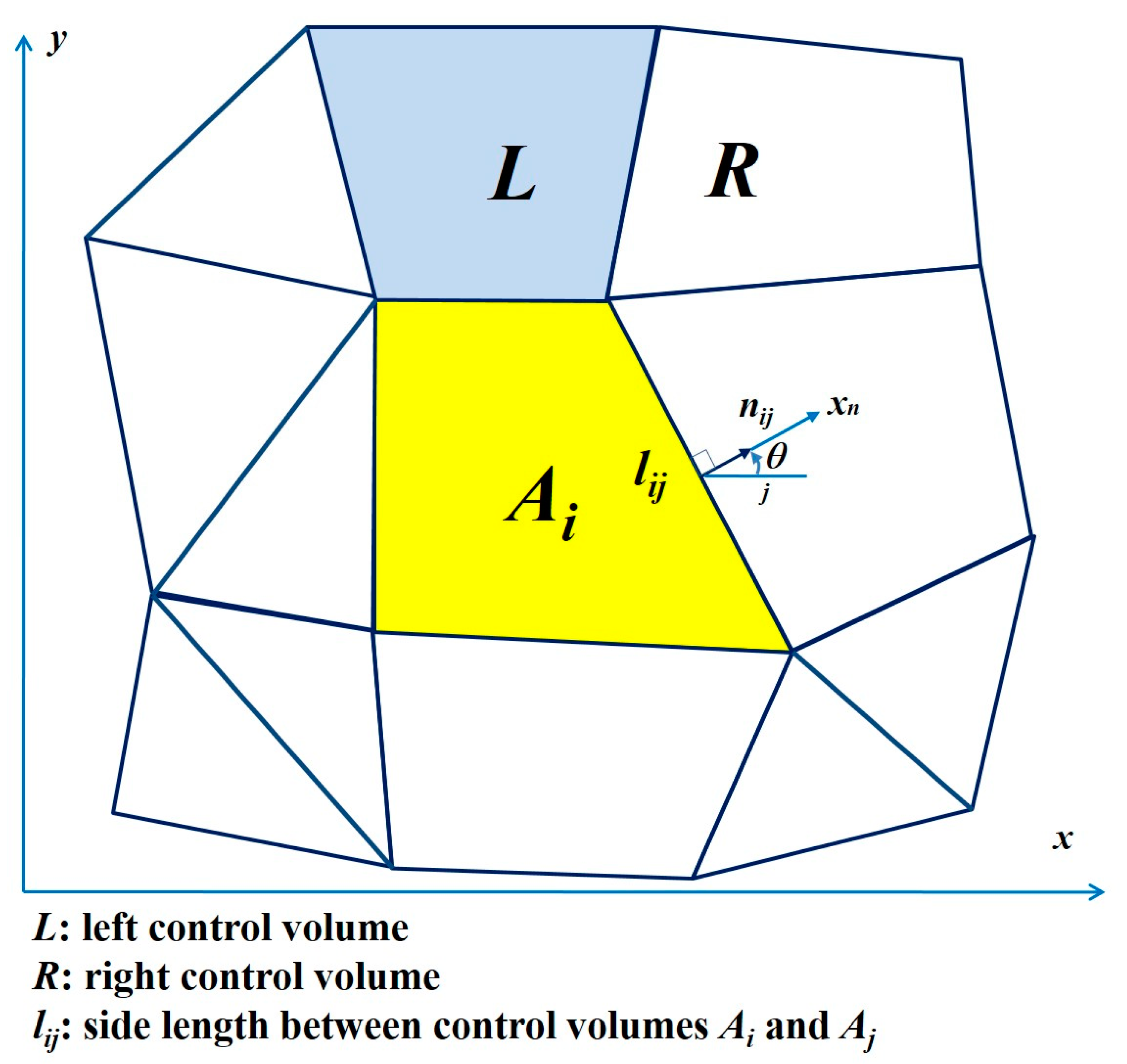
The numerical scheme applied in this study is a finite volume method that calculates the flux through the boundary of a cell or a control volume consisting of a computational domain. The integration of Equation (1) over an arbitrary triangular or quadrilateral cell, $A_i$ as shown in Figure 1 yields the following equation in vector forms:

$${{\displaystyle \int }}_{A_i}\frac{\partial \mathit{U}}{\partial t}d\mathsf{\Omega }+{{\displaystyle \oint }}_{\partial A_i}\mathit{F}\left(\mathit{U}\right)·{\mathit{n}}_{i}ds={{\displaystyle \int }}_{A_i}S\left(\mathit{U}\right)$$

(5)

where $\mathit{F}={\left(\mathit{E}, \mathit{H}\right)}^T$, $\partial A_i$ is the boundary of a cell and ${\mathit{n}}_i$ is the outward unit normal vector.

The discretized form of Equation (5) is given for the cell $A_i$ as follows:

$$\left|A_i\right|\frac{d\mathit{U}}{dt}=-{\displaystyle \sum }_{j=1}^m\mathit{F}\left(\mathit{U}\right)·{\mathit{n}}_{ij}{L}_{ij}+\left|A_i\right|{\mathit{S}}_i\left(\mathit{U}\right)$$

(6)

where $\left|A_i\right|$ is the surface area of the cell $A_i$ and m is the number of the sides of the cell $A_i$ (m = 3 for a triangular cell and m = 4 for the quadrilateral cell), $L_{ij}$ is the length of side j in the cell $A_i$, and $n_{ij}$ is the outward unit normal vector from side j.

The finite volume method directly allows the spatial discretization by introducing the property of the rotational invariance [23]. If this property is applied to the flux terms in Equation (6), the calculation of the flux terms are reduced to the one-dimensional problem and these terms can be written as follows:

$$\mathit{F}\left(\mathit{U}\right)·{\mathit{n}}_{ij}=T_{n_{ij}}^{-1}G\left(T_{n_{ij}}\mathit{U}\right)$$

(7)

where $T_{n_{ij}}$ is the transformation matrix expressed by Equation (8):

$$T_{n_{ij}}=\left[\begin{array}{ccc}1& 0& 0\\ 0& \cos {\theta }_{ij}& \sin {\theta }_{ij}\\ 0& -\sin {\theta }_{ij}& \cos {\theta }_{ij}\end{array}\right]$$

(8)

By substituting Equation (8) into Equation (7), the following equation can be obtained for the cell $A_i$:

$$\left|A_i\right|\frac{d{\mathit{U}}_i}{dt}=-{\displaystyle \sum }_{j=1}^m{T}_{n_{ij}}^{-1}G\left(T_{n_{ij}}{\mathit{U}}_i, T_{n_{ij}}{\mathit{U}}_j\right)L_{ij}+\left|A_i\right|{\mathit{S}}_i\left({\mathit{U}}_i\right)$$

(9)

where $G\left(T_{n_{ij}}{\mathit{U}}_i, T_{n_{ij}}{\mathit{U}}_j\right)=\tilde{G}\left(U_L, U_R\right)$ is the flux at the boundary of the cell $A_i$ and resolved from an approximate solver of the Riemann problem having a left state variable $U_L$ and a right state variable $U_R$ for the cells L and R in Figure 1.

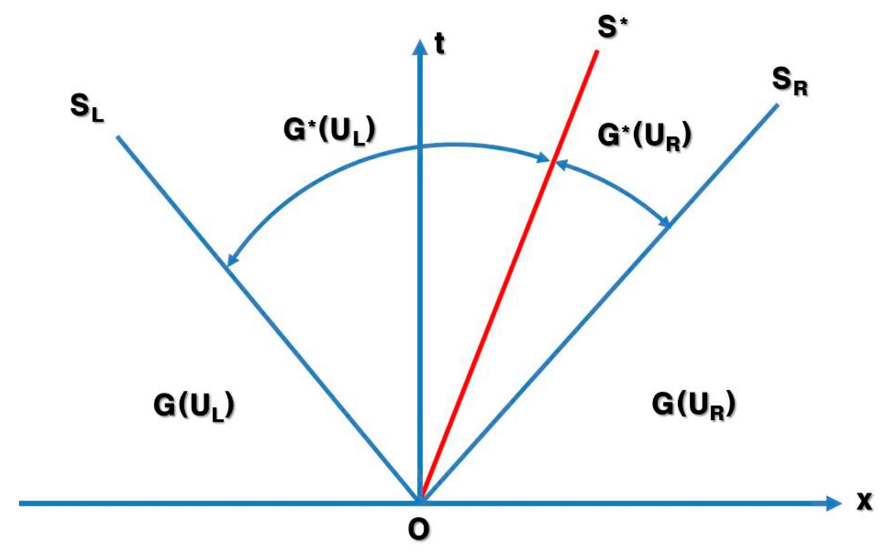
In this study, the HLLC algorithm proposed by Billet and Toro [24] is employed to compute the flux terms. This algorithm has the first-order accuracy both in time and space and an improved version of the HLL scheme [25]. Unlike the HLL algorithm which considers only two wave speeds $S_L$ and $S_R$, the HLLC algorithm introduces the intermediate wave speed $S^{*}$ between two wave speeds, as shown in Figure 2. In the HLLC algorithm, the flux terms in Equation (9) can be expressed as follows [23,26]:

$$\tilde{G}\left(U_L, U_R\right)\approx G^{HLLC}\left(U_L, U_R\right)=\{\begin{array}{ccc}G\left(U_L\right)& \mathrm{if}& S_L\ge 0\\ G\left(U_L^{*}\right)& \mathrm{if}& S_L<0\le S^{*}\\ G\left(U_R^{*}\right)& \mathrm{if}& S^{*}<0\le S_R\\ G\left(U_R\right)& \mathrm{if}& S_R\le 0\end{array}$$

(10)

where $G\left(U_L^{*}\right)$ and $G\left(U_R^{*}\right)$ can be determined by:

$$\begin{array}{c}G\left(U_L^{*}\right)=G\left(U_L\right)+S_L\left(U_L^{*}-U_L\right)\\ G\left(U_R^{*}\right)=G\left(U_R\right)+S_R\left(U_R^{*}-U_R\right)\end{array}$$

(11)

where,

$$U_k^{*}=h_k\left(\frac{S_k-u_k}{S_k-S^{*}}\right)\left(\begin{array}{c}1\\ S^{*}\\ v_k\end{array}\right), k=L, R$$

(12)

The wave speeds $S_L$, $S^{*}$ and $S_R$ in Equation (10) can be calculated from:

$$\begin{array}{c}{S}_L=min\left(u_L-\sqrt{g{h}_L}, u^{*}-\sqrt{g{h}^{*}}\right)\\ S^{*}=u^{*}=\frac{u_L+u_R}{2}+\sqrt{g{h}_L}-\sqrt{g{h}_R}\\ S_R=max\left(u_R+\sqrt{g{h}_R}, u^{*}+\sqrt{g{h}^{*}}\right)\end{array}$$

(13)

where,

$$h^{*}=\frac{\left(u_L+2\sqrt{g{h}_L}-u_R-2\sqrt{g{h}_R}\right)}{16}$$

(14)

When the HLLC algorithm is applied to the river flow with an abrupt and irregular bed geometry, it is difficult to obtain accurate results for the flow analysis because of the numerical oscillation due to the imbalance between the flux and source terms [27]. To resolve this problem, the bed slope is directly considered to calculate $G\left(U_R\right)$ in Equation (10) in this study [22,28]:

$$G^s=G\left(U_R\right)+\left[\begin{array}{c}0\\ \frac{1}{2}g\left(h_L+h_R\right)\left(z_{b,R}-z_{b,L}\right)\\ 0\end{array}\right]$$

(15)

where $z_{b,R}$ and $z_{b,L}$ are the bed elevations at the cells R and L, respectively.

When Equation (15) is considered, Equation (9) can be expressed as follows:

$$\left|A_i\right|\frac{d{\mathit{U}}_i}{dt}=-{\displaystyle \sum }_{j=1}^m{T}_{n_{ij}}^{-1}{G}^{HLLC,s}\left({\mathit{U}}_i, {\mathit{U}}_j\right)L_{ij}+\left|A_i\right|{\mathit{S}}_i^f\left({\mathit{U}}_i\right)$$

(16)

where ${\mathit{S}}_i^f\left({\mathit{U}}_i\right)$ is the friction term and can be written by:

$${\mathit{S}}_i^f\left({\mathit{U}}_i\right)=-g\frac{n^2\sqrt{u_L^2+v_L^2}}{h^{4/3}}\left[\begin{array}{c}0\\ u_L\\ v_L\end{array}\right]$$

(17)

In order to compute the water depth and velocity with time, a simple explicit Euler scheme is adopted in this study and can be written as follows:

$${\mathit{U}}_i^{n+1}={\mathit{U}}_i^n-\frac{\mathsf{\Delta }t}{\left|A_i\right|}{\displaystyle \sum }_{j=1}^m{T}_j^{-1}{G}^{HLLC,s}\left({\mathit{U}}_L^n, {\mathit{U}}_R^n\right)+\mathsf{\Delta }t{\mathit{S}}_i^{f,n}\left({\mathit{U}}_i\right)$$

(18)

where ${\mathit{U}}_i^n$ and ${\mathit{U}}_i^{n+1}$ are the approximation of ${\mathit{U}}_i$ computed at times $t^n$ and $t^{n+1}$, respectively, and ${\mathit{S}}_i^{f,n}\left({\mathit{U}}_i\right)$ is the value of ${\mathit{S}}_i^f\left({\mathit{U}}_i\right)$ computed at time $t^n$.

It is well known that the simple explicit Euler scheme is very efficient for the repetitive computation in the system of non-linear equations, such as shallow-water equations. However, it is necessary to satisfy the CFL (Courant–Freidrichs–Lewy) condition to achieve the numerical stability. The condition is expressed by Loukili and Souhaimani [29]:

$$\mathrm{CFL}=\mathsf{\Delta }t\frac{max\left(\sqrt{gh}+\sqrt{u_L^2+v_L^2}\right)}{min\left(d_{C,LR}\right)}$$

(19)

where $d_{C,LR}$ is the distance between the center of cell and the center of the interface of cells R and L.

In this study, the wet and dry bed situations are dealt with the analytical method given as Toro [23]:

$$\begin{array}{cccc}{S}_L=u_R-2\sqrt{g{h}_R},& S_R=u_R+2\sqrt{g{h}_R},& S^{*}=S_L& \mathrm{if} h_L=0\\ S_L=u_L-2\sqrt{g{h}_L},& S_R=u_L+2\sqrt{g{h}_L},& S^{*}=S_R& \mathrm{if} h_R=0\end{array}$$

(20)

Equation (20) is very efficient for the flat bed (i.e., $\mathsf{\Delta }{z}_b=0$). If $\mathsf{\Delta }{z}_b\ne 0$, however, the solution becomes numerically unstable [30]. To resolve the problem, a minimum water depth h_m (>0) is introduced. If the water depth is less than $h_m$, the dry bed condition is imposed and the velocity is set at zero. In general, the range of $h_m$ is between 1.0 × 10⁻⁶–1.0 × 10⁻³ m. In this study, the value of 1.0 × 10⁻³ m is chosen for an irregular bed geometry [30].

3. Field Application to Flood Inundation in a Small-Scale Coastal Urban Area

3.1. Target Area: Gohyun River Basin

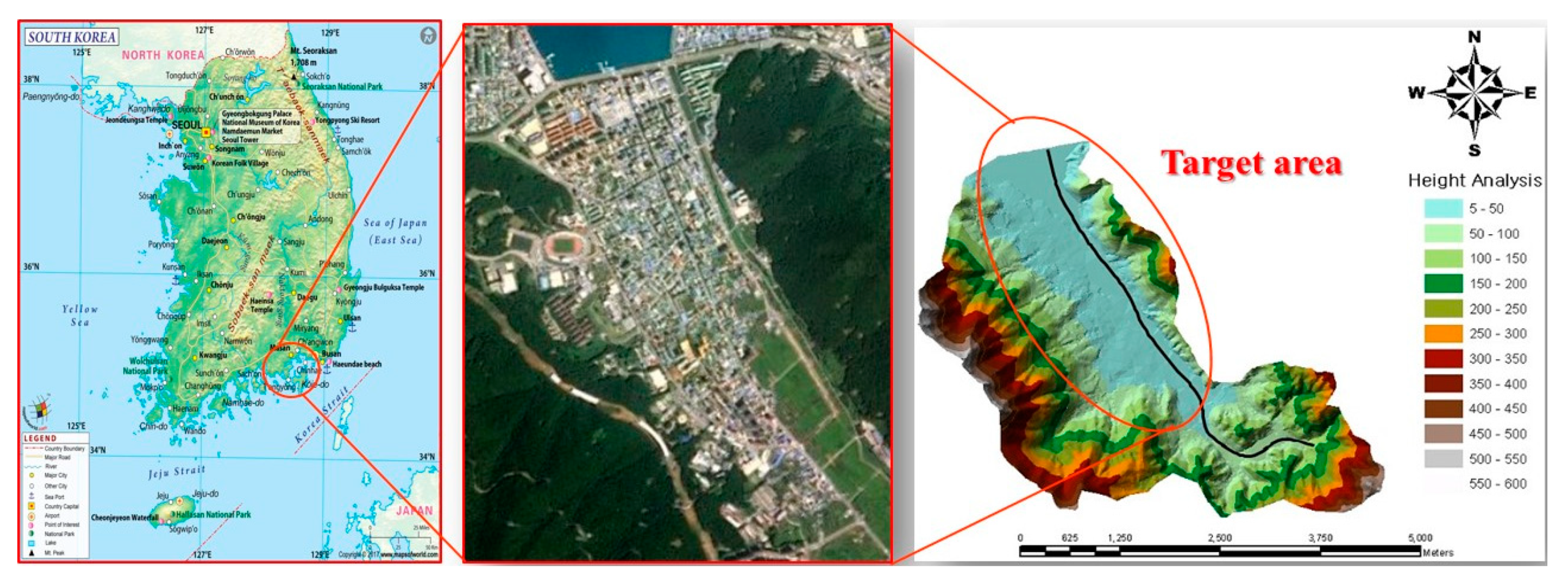
The Gohyun river basin is located in Shinhyeon-eup, Geoje-si, Gyeongsangnam-do, South Korea. The area of the Gohyun river basin is 15.38 km², and its average width of the basin is 1.1–2.3 km. The length of the Gohyun river is 5.1 km. The Gyeryongsan mountain, which rises EL. 566 m above sea level, is located in the southwest of the basin and the Dokbongsan mountain, which rises EL. 350 m above sea level, is located in the northeast part. The source of the water supply is a local class-2 river that originates at the foot of the Mundong waterfall, which is the uppermost river, and flows down to the east-west to reach the Mundong reservoir. It then flows through the Mundong reservoir to the northeast to pass Shinhyeon 1 and 2 bridges in the urban area of Shinhyeon-eup, and finally flows to Gohyun bay. Figure 3 shows a satellite photo of the Gohyun river basin, a map of the basin, and the target area. The highest elevation in the area is EL. 119.02 m, and the elevation of the downstream of the Gohyun river, which is adjacent to Gohyun bay, is EL. 0.74 m.

Typhoon “Maemi” was the most powerful one to strike South Korea since record-keeping began in 1904. When this typhoon with the lowest pressure of 950 hPa and the highest wind of 215 km/h passed the southern coast of South Korea on 10 September 2003, it caused heavy rainfall that peaked at 401.5 mm [31]. On 13 September 2003, the protected lowland in the Gohyun river basin was flooded owing to the intensive rainfall and the high tidal level caused by Typhoon “Maemi”, such that more than 300 houses and shopping arcades in the urban area located downstream were flooded. Even after Typhoon “Maemi”, flood damage has been occurring regularly in the same area when the water level of the Gohyun river rises owing to heavy rains. This is because the drainage of the inner basin is poor when the tide level exceeds the elevation of the riverbed in the downstream area of the Gohyun river.

3.2. HEC-HMS (Hydrologic Engineering Center-Hydrologic Modeling System) Model

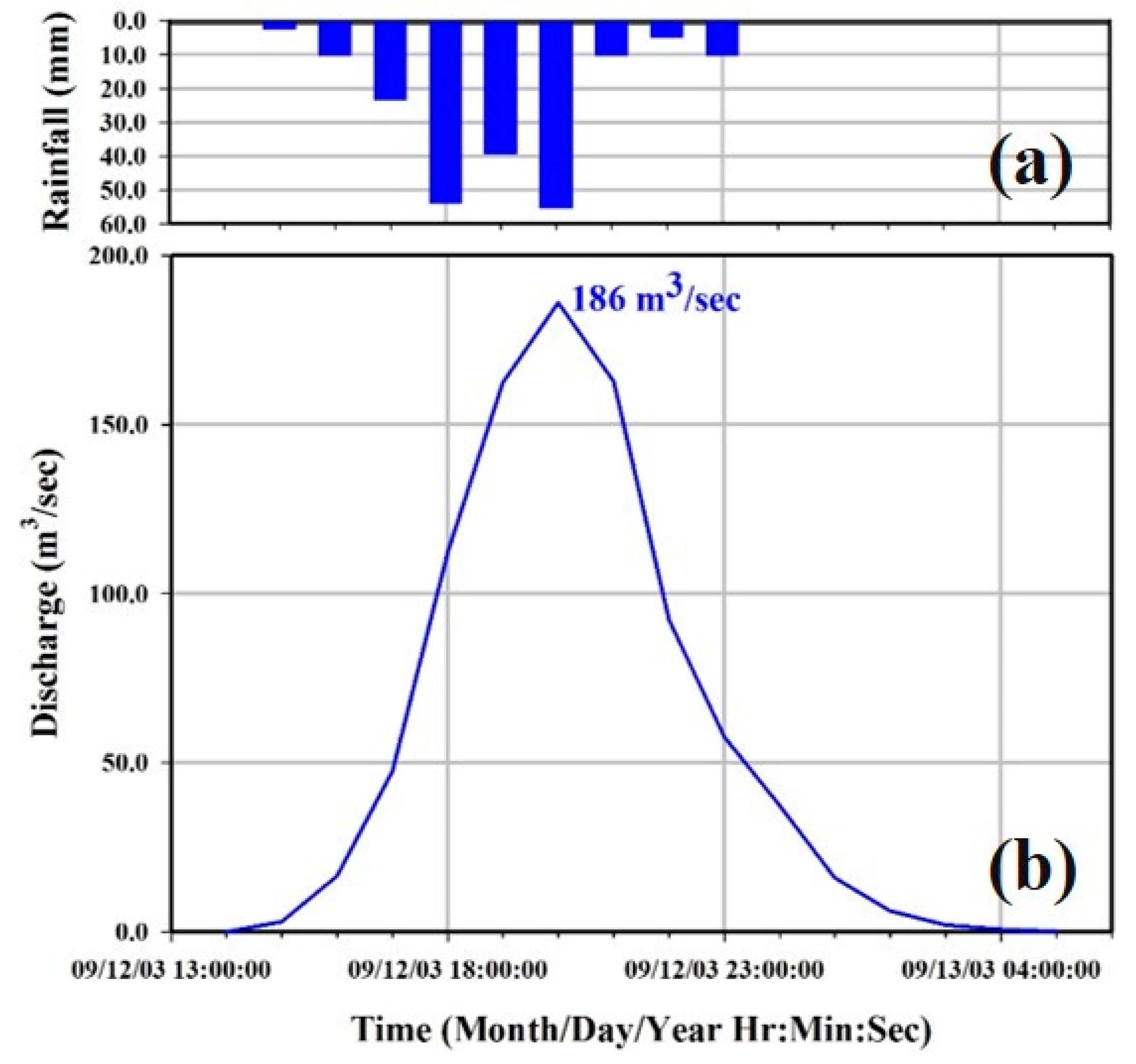
Figure 4a shows the temporal distribution of the rainfall from 1:00 p.m. on 12 September to 5:00 a.m. on 13 September 2003 observed hourly at the Gohyun weather station of Korea Meteorological Administration (KMA) [31]; this includes the time when the maximum amount of rainfall was observed during the period of occurrence of Typhoon “Maemi”. Because there was no measurement data for the flood amount generated in Gohyun river, the flood hydrograph corresponding to the measured temporal distribution of rainfall is estimated using the HEC-HMS (Hydrologic Engineering Center-Hydrologic Modeling System) software [32] with the land-use analysis data [33].

The HEC-HMS is physically based and conceptually semi-distributed model designed to simulate rainfall–runoff processes in a wide range of geographic areas, from large river basin water supplies and flood hydrology to small urban and natural watershed runoffs [32]. HEC-HMS has become very popular and been adopted in many hydrological studies because of its ability in the simulation of runoff both in short- and long-term events, its simplicity to operate, and use of common methods [34]. In this study, the Soil Conservation Service curve number (SCS-CN), Clark unit hydrograph, and Muskingum routing methods are selected for each component of the runoff process as runoff depth, direct runoff, and channel routing respectively. The baseflow is not considered because in short duration event modelling and for small sub-basins the contribution of base flow is insignificant for flood flows [35].

The SCS-CN model assumes that the accumulated rainfall-excess depends upon the cumulative precipitation, soil type, land use and the previous moisture conditions as estimated in the following relationship [36]:

$$P_e=\frac{{\left(P-I_a\right)}^2}{P-I_a-S}$$

(21)

where $P_e$ is the accumulated precipitation excess at time t (mm), P is the accumulated rainfall depth at time t (mm), $I_a$ is the initial abstraction (initial loss) (mm) = $\mathsf{\alpha }S$, α is 0.2 as a standard, and S is the potential maximum retention (mm), a measure of the ability of a watershed to abstract and retain storm precipitation.

The maximum retention, S, and watershed characteristics are related through an intermediate dimensionless parameter, the curve number (CN) as:

$$S=\mathrm{25,400}-\frac{254 CN}{CN}$$

(22)

where CN is the SCS curve number used to represent the combined effects of the primary characteristics of the catchment area, including soil type, land use, and the previous moisture condition. The CN values range from 100 (water bodies) to approximately 30 for permeable soils with high infiltration rates [6]. The CN is calculated as 93.56 under the condition of AMC-III (

Table 1. Curve number (CN) value calculated in this study.

Basin	Area (km2)	Length (km)	Mean Slope (m/m)	CN (AMC-III)
Gohyun river	15.38	5.1	1/350	93.56

).

The transform prediction models in HEC-HMS simulate the process of the direct runoff of excess precipitation on the watershed, and they transform the precipitation excess into point runoff. The models transform the rainfall excess into direct surface runoff through a unit hydrograph, and the Clarks unit hydrograph method is used as the transform models in this study. The basic concepts and assumptions behind each hydrologic method can be also found in the HEC-HMS technical manual [36]. Moreover, Rziha, Kraven II and Kirpich methods shown in Equations (23)–(25) and a relation shown in Equation (26) are also jointly applied in this study for estimating the initial values for the time of concentration $\left(t_c\right)$ and lag time $\left(t_l\right)$ for the Gohyun river basin, which are used as input data in the selected transform methods:

$$t_c=0.833 \frac{L}{S{P}^{0.6}}\left(\mathrm{river}\mathrm{having}SU>1/200\right)$$

(23)

$$t_c=16.667\frac{L}{V}(SD>1/100,V=3.5\mathrm{m}/\mathrm{s};1/200\le SD\le 1/100,V=3.0\mathrm{m}/\mathrm{s}; SD<1/200,V=2.1 \mathrm{m}/\mathrm{s})$$

(24)

$$t_c=3.976\frac{L^{0.77}}{M{S}^{0.385}}(\mathrm{small}\mathrm{agricultural}\mathrm{land})$$

(25)

$$t_l=0.6t_c$$

(26)

where SU and SD are the river upstream and downstream mean slope(m/m), respectively, L is the reach length in km, V is the overland flow velocity in m/s, and MS is the mean slope in m/m. The SU and SD of Gohyun river are 1/109 and 1/591.

Table 2. $t_c$ and $t_l$ calculated in this study.

Basin	Time of Concentration (tc, hr)				Lag Time (tl, hr)
	Rziha	Kraven II	Kirpich	Mean Value
Gohyun river	1.18	0.67	2.22	1.36	0.81

shows the time of concentrations calculated from three different methods. In this study, the mean value of these three methods is used because there is no measured data related to the time of concentration in the Gohyun river basin.

Figure 4b exhibits the estimated flood hydrograph. The maximum rainfall was 55.4 mm, which was observed at 8 p.m. on 12 September and the maximum calculated discharge was 186 m³/s.

3.3. Flood Inundation Model Application

Urban flood models fall in one of the following four categories depending on the method of representing buildings in the terrain [37]: (1) building-hole models, where the buildings are replaced with building-perimeter polyline [9], and either a free-slip boundary [38] or other internal hydraulic conditions are imposed along the perimeter, (2) building-resistance models, where a relatively large resistance parameter (bottom friction) is assigned to cells corresponding to building footprints [39] or developed parcels; building-porosity models, where buildings are represented through spatially-distributed porosity and drag coefficients, without resolving the exact geometry of the buildings [40]; and (3) building-block models, where buildings with their representative shape and height are included in the terrain, essentially blocking the flow from passing through them [41].

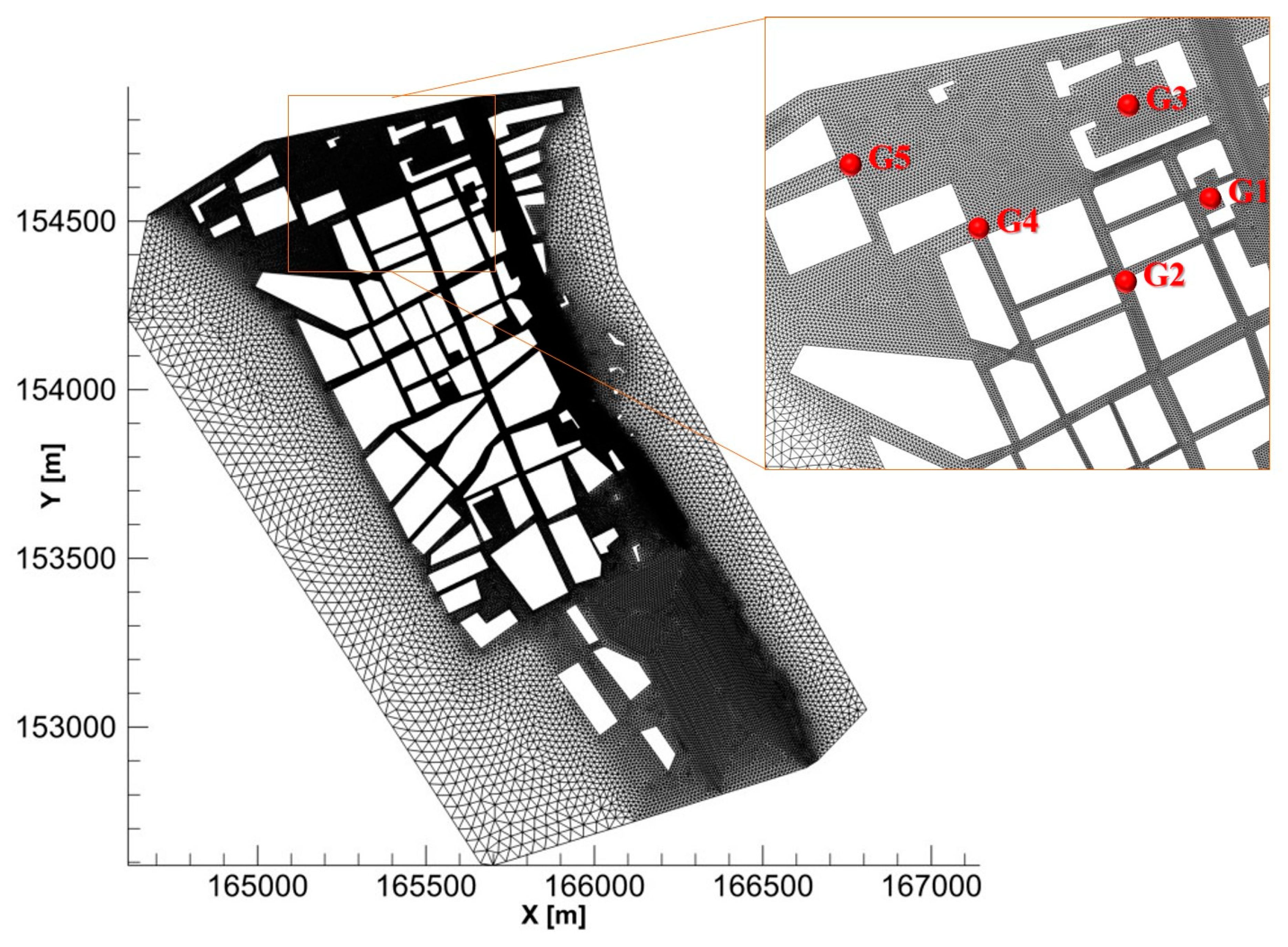
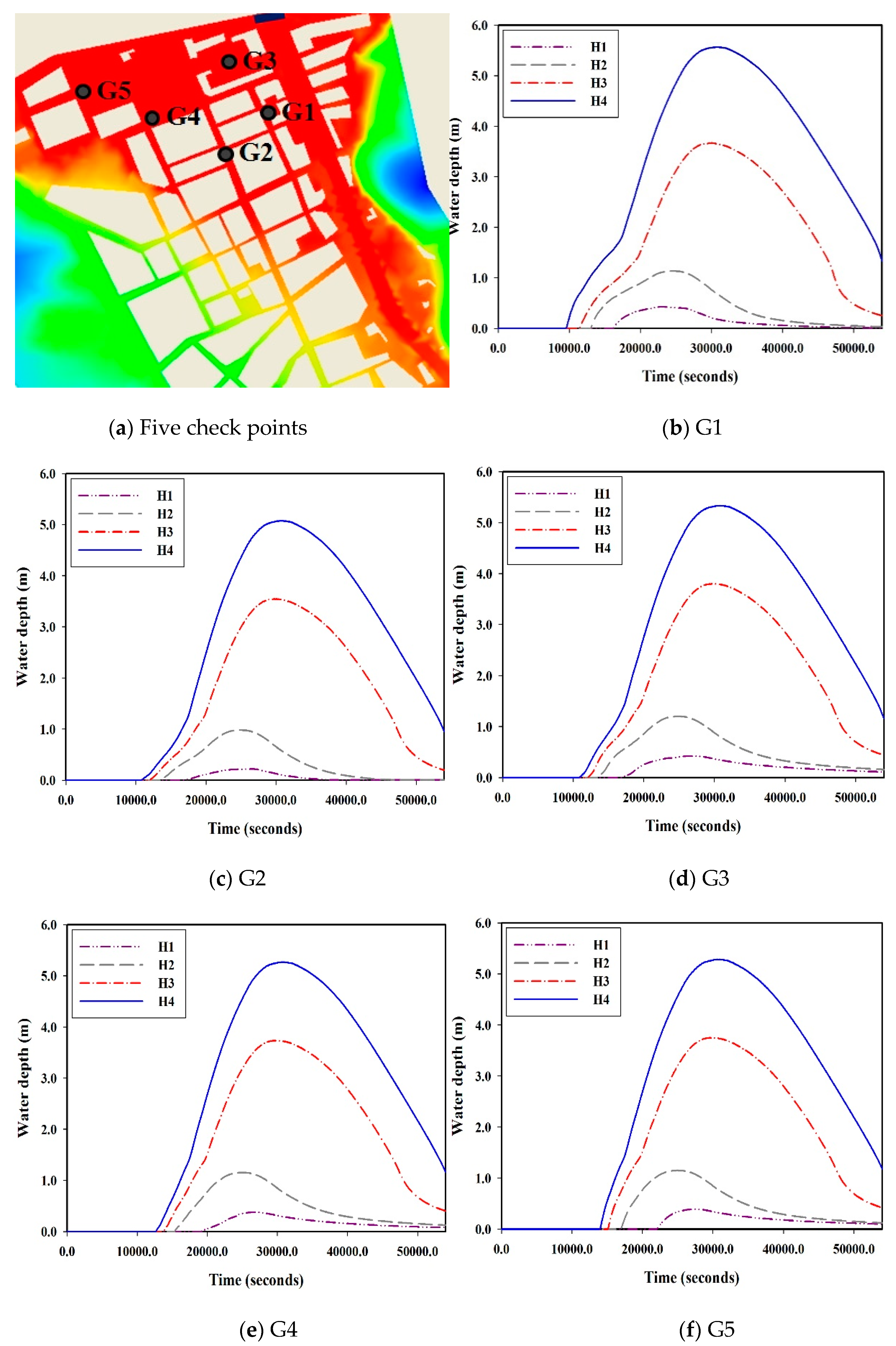
In this study, the buildings in the urban area are represented by the concept of the building-hole model and Figure 5 shows an unstructured grid system constructed around the downstream urban area of the Gohyun river. The grid system consists of 42,893 nodes and 79,598 cells. In addition, five check points, from G1 to G5, are selected in order to observe the changes in the inundated water depths with time calculated for the urban area. The reason for choosing these five points is to investigate the temporal variation of inundation depths at the points where an abrupt change of the flood wave can be expected. The point G1 is located at the nearest position from the river and the point G2 is located at the road in the building blocks. The point G3 corresponds to the position located in the center of the small square in the vicinity of the river and the point G4 is located at the position connected with the square area and roads. The point G5 is located at the farthest position from the river and is connected to the road between two buildings.

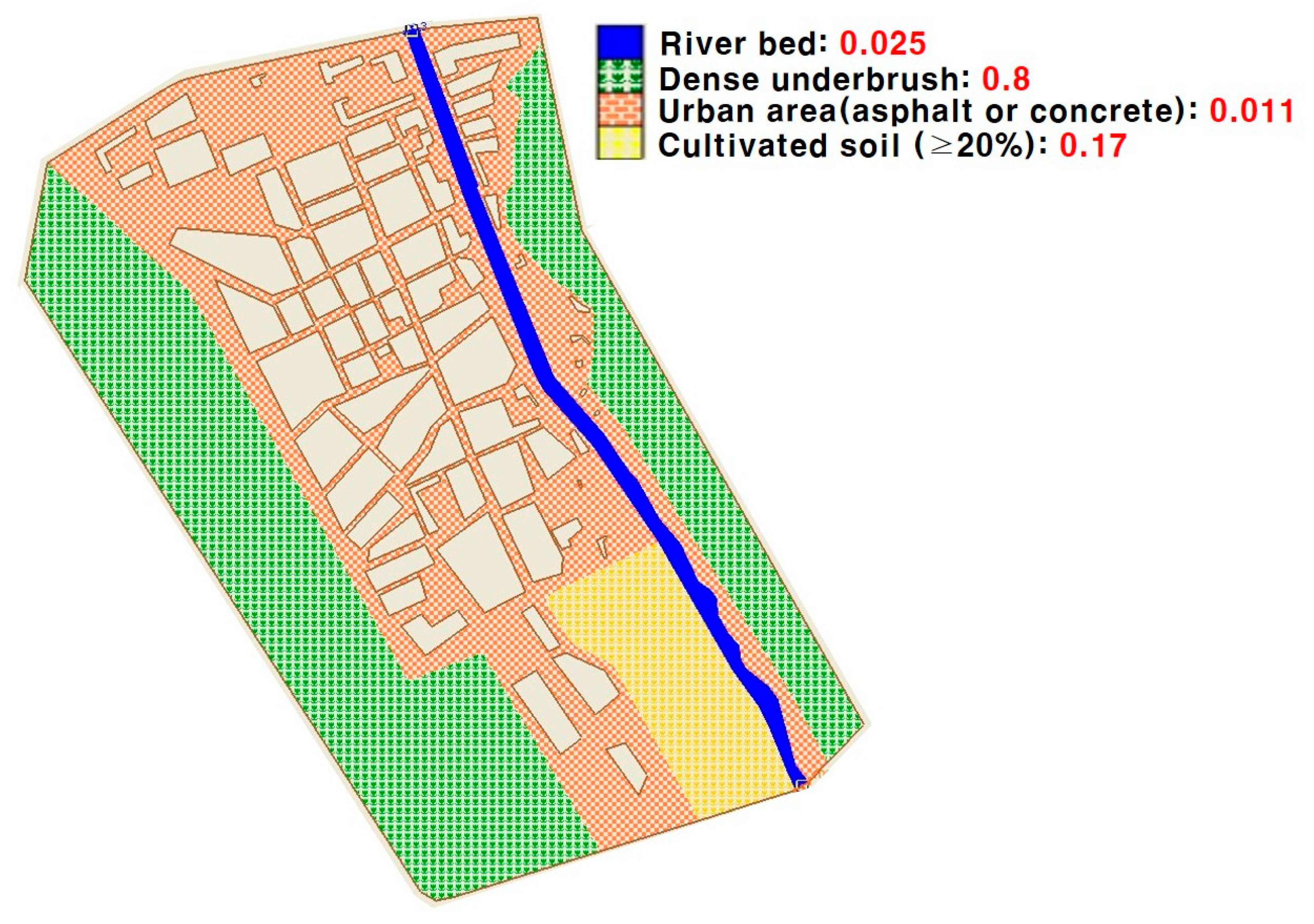
In the present study, in Case 1 different values of Manning’s roughness coefficient (n) of the target area divided according to the land use map of scale 1:5000 provided from the National Geographic Information Institute of Korea [42] are used, whereas in Case 2, the average value of n is applied to all the areas except the Gohyun riverbed. In Case 1, because the Gohyun river is a natural stream, n = 0.025 corresponding to the natural riverbed [43] is applied. The n values in the remaining areas are assigned according to those of the land uses listed in

Table 3. Manning’s roughness coefficients (n) for overland flow [44].

Surface Description	n
Smooth surfaces (concrete, asphalt, gravel, or bare soil)	0.011
Fallow (no residue)	0.050
Cultivated soils
Residue cover ≤ 20%	0.060
Residue cover ≥ 20%	0.170
Grass
Short grass prairie	0.150
Dense grasses	0.240
Bermuda grass	0.410
Range (natural)	0.130
Woods
Light underbrush	0.400
Dense underbrush	0.800

.

The building groups existing in the urban area are considered as impervious areas and flood flows are considered to occur only through the roads between the buildings. Accordingly, the roads are assumed to be smooth ground surfaces made of asphalt or concrete, to which n = 0.011 is applied. The cultivated soils are applied with n = 0.17 because the residue cover exceeds 20%, whereas the forests are applied with n = 0.8 because of their associated dense underbrush [44]. Figure 6 shows the distribution of Manning’s roughness coefficients assigned according to the land uses in the target area for Case 1. In Case 2, the value of n = 0.025 as in Case 1 is applied to the Gohyun riverbed and for the remaining areas, the average value of n is 0.327 (= 0.8 for dense underbrush +0.011 for urban area +0.17 for cultivated soil with residue cover ≥20%/3). However, because this average value of n is strongly influenced by the value of n for the dense underbrush and the inundation due to the river flooding actually did not reach the forest area with dense underbrush, the average value of n = 0.0905 for the urban area and cultivated soil with residue cover ≥ 20% is applied in Case 2. However, because this average value of n is not the optimal value to reflect the actual inundation situation at that time, the simulations to find the optimal value of n are performed with the range from n = 0.011 for the urban area to 0.0905 for the average value of n.

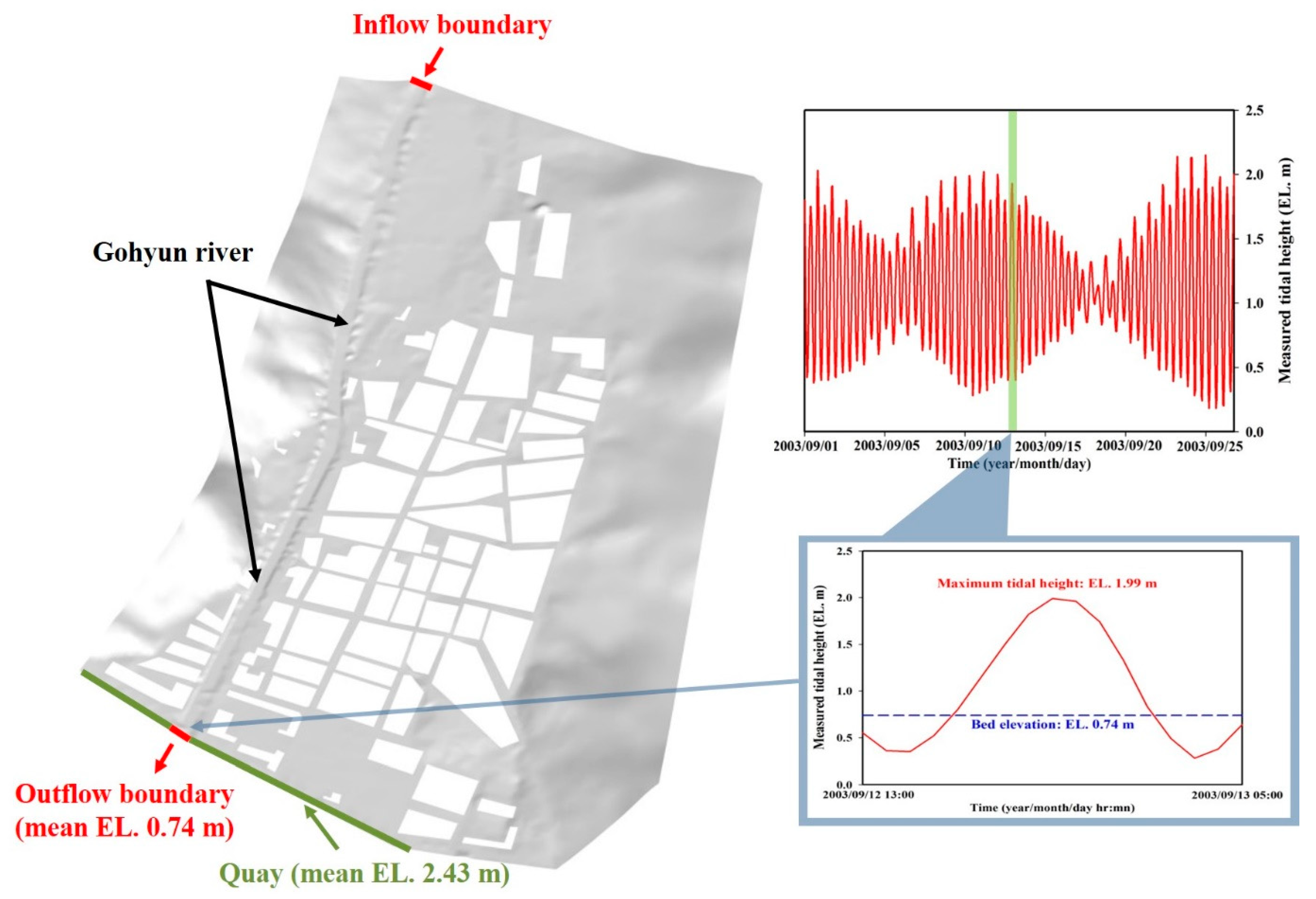
The inflow boundary condition is applied to the upstream boundary of the Gohyun river, and the flood hydrograph shown in Figure 4 is used. In terms of the outflow boundary condition, the data observed at the Gadeokdo Tidal Observatory, which is closest to Gohyun bay, are applied to the downstream boundary because there are no observed tidal level record data for Gohyun bay during the period of Typhoon “Maemi”. The maximum tide level is observed at 7:00 p.m. on 12 September 2003, and it is EL. 1.99 m. As shown in Figure 7, because the elevation of the quay of Gohyun port is EL. 2.43 m on average, which is about EL. 0.35 m higher than the maximum tide level, the tides do not overflow and flow into the urban area.

The total simulation time is 54,000 s (the duration from 1:00 p.m. on 12 September 2003 to 5:00 a.m. on 13 September 2003 converted into units of seconds), and a value of 0.75 is applied as the CFL condition.

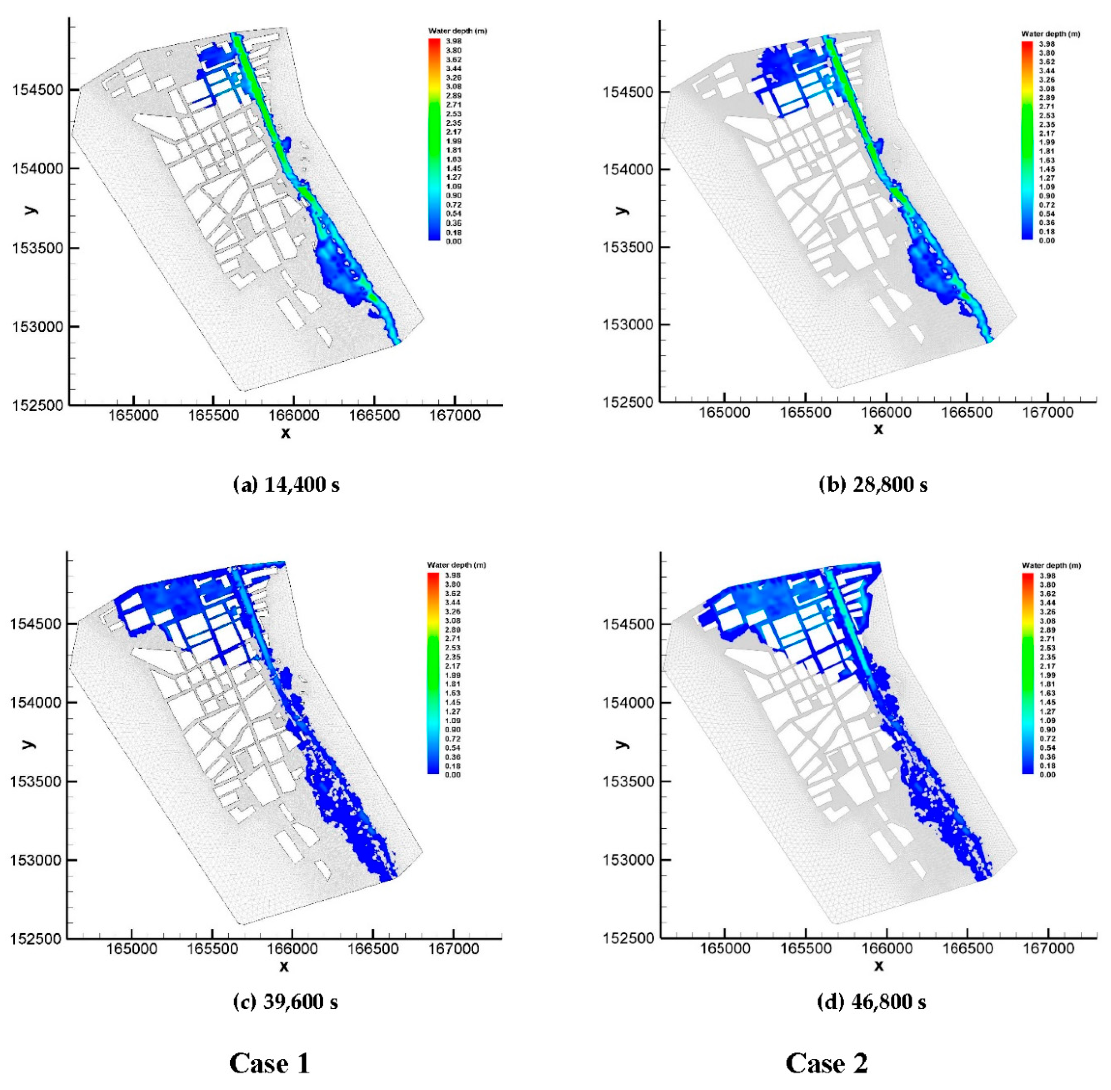
Figure 8 shows the comparison of the spatial distributions of the inundated water depths with time for Cases 1 and 2. It can be seen that the flood enters from the upstream boundary flow along the river, and overflows, and moves into the urban area owing to the poor drainage to the sea since the time when the tide level becomes higher than the elevation of the riverbed at the downstream boundary. The highest inundated water depth occurs at 39,600 s of the total simulation time of 54,000 s, and the inundated water depth gradually decreases thereafter owing to the decreases in the inflow.

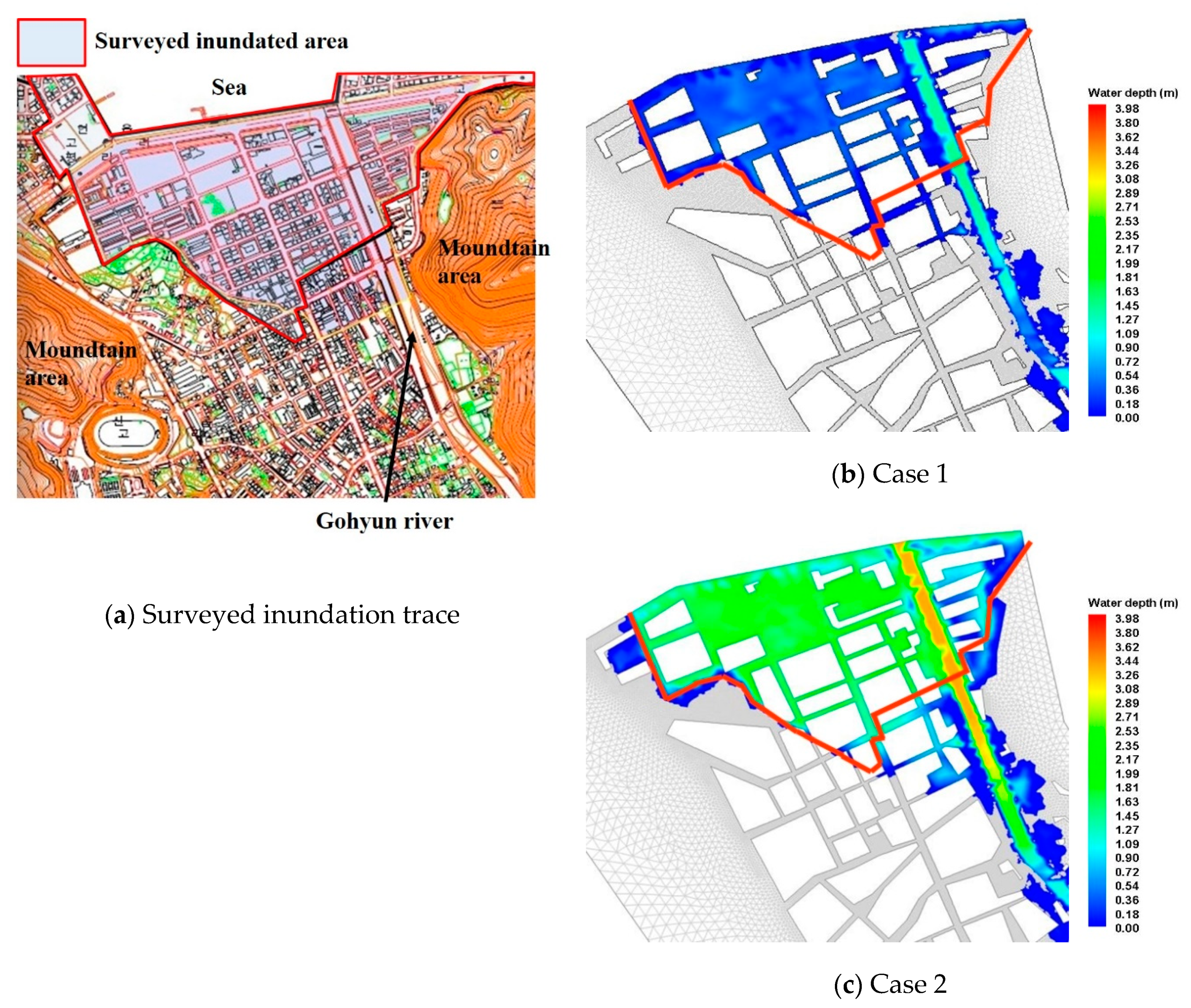
Figure 9a shows the digital map (scale 1:5000) of the actual inundation trace surveyed in the field from 22 September to 6 October 2013 after the urban area at the downstream of the Gohyun river was flooded during Typhoon “Maemi” [3]. The flooded area was 0.43 km², and the range of the inundated water depths was 0.25–1.00 m. Figure 9b,c show the spatial range of the inundated water depths and flooded area at 39,600 s for Cases 1 and 2.

Table 4. Comparison of the inundated water depths and areas for Cases 1 and 2 with the surveyed inundated trace.

Item	Surveyed Inundated Trace	Case 1	Case 2
Inundated water depth (m)	0.25–1.00	0.30–1.15	1.10–2.80
Inundated area (km2)	0.43	0.48	0.55

compares the results of the simulations of the two cases using the surveyed inundated trace. In Case 1, in which the distribution of Manning’s roughness coefficients is according to the land uses, the flooded area is 0.48 km² and the range of the inundated water depths is 0.30–1.15 m, which relatively well coincide with the inundation trace data. However, in Case 2, in which the Manning’s roughness coefficients are uniform, around 0.025, for all the areas except the riverbed, the range of the inundated water depths is 1.1–2.8 m and the flooded area is 0.55 km². Therefore, it can be seen that these values in Case 2 are relatively overestimated compared to those in Case 1.

4. Simulation of the Flood Inundation according to the Changes in the Flood Inflow Rate

4.1. Flood Inflow Rate Scenarios

For the Gohyun river, one of the major causes of the regular occurrence of flood inundation in the urban areas is that the discharge capacity (design discharge capacity: 58 m³/s) of the river where it is in contact with the sea is significantly insufficient to drain very large floods (maximum flood amount: 183 m³/s) generated during the typhoon “Maemi”. Moreover, the inland water is not smoothly drained into the sea when the tide levels become higher than the elevation of the riverbed or when massive floods occur upstream (Figure 10).

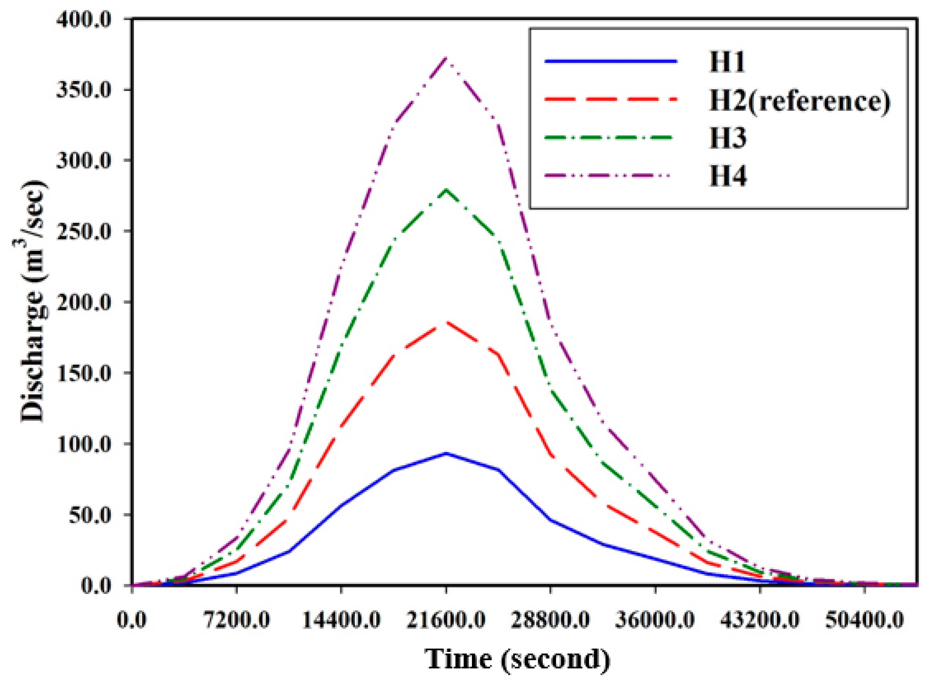
Reflecting these flood characteristics and using the flood hydrograph (H2) calculated assuming that the tidal level data during the period Typhoon “Maemi” are applied to the downstream boundary of the Gohyun river, four scenarios are constructed. These are simply based on flood inflow rates of 0.5 times (H1), 1.5 times (H3), and 2.0 times (H4) of the reference case H2 because the Gohyun river basin is unmeasured and the temporal data to apply to the extreme analysis or the frequency analysis of the intense rainfall and the flood inflow rate were not sufficient. These scenarios of the flood inflow rate are applied to simulate and analyze the flood flows in the urban areas downstream of the Gohyun river. As shown in Figure 11, the maximum flood inflow rates for the individual scenarios are 94 m³/s for H1, 274 m³/s for H3, and 382 m³/s for H4. The simulation conditions are the same as those employed for the field verification of the model presented above.

4.2. Comparison of the Calculated Inundated Water Depths and Flooded Areas

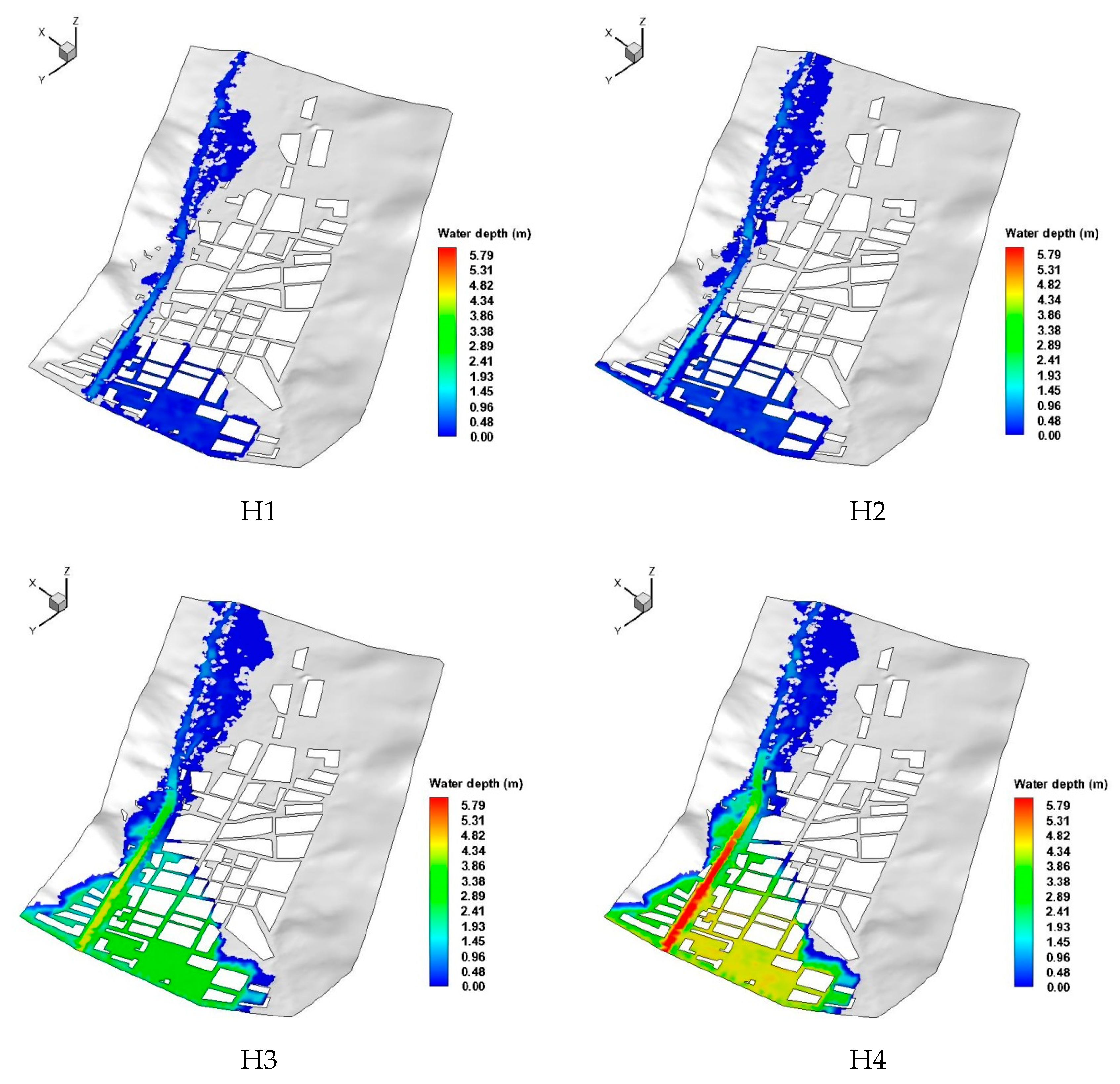
Figure 12 shows the spatial distributions of the inundated water depth when they are calculated to be the highest for each case based on the four scenarios of flood inflow rates. It can be seen that as the flood inflow rate increases, the flooded area and inundated water depth increases. In particular, it can be seen that in the case of H3 and H4, the inland water is not appropriately drained into the sea because the width of the Gohyun river, which is connected to Gohyun bay, is narrow, so that relatively high inundated water depths are maintained in the urban area.

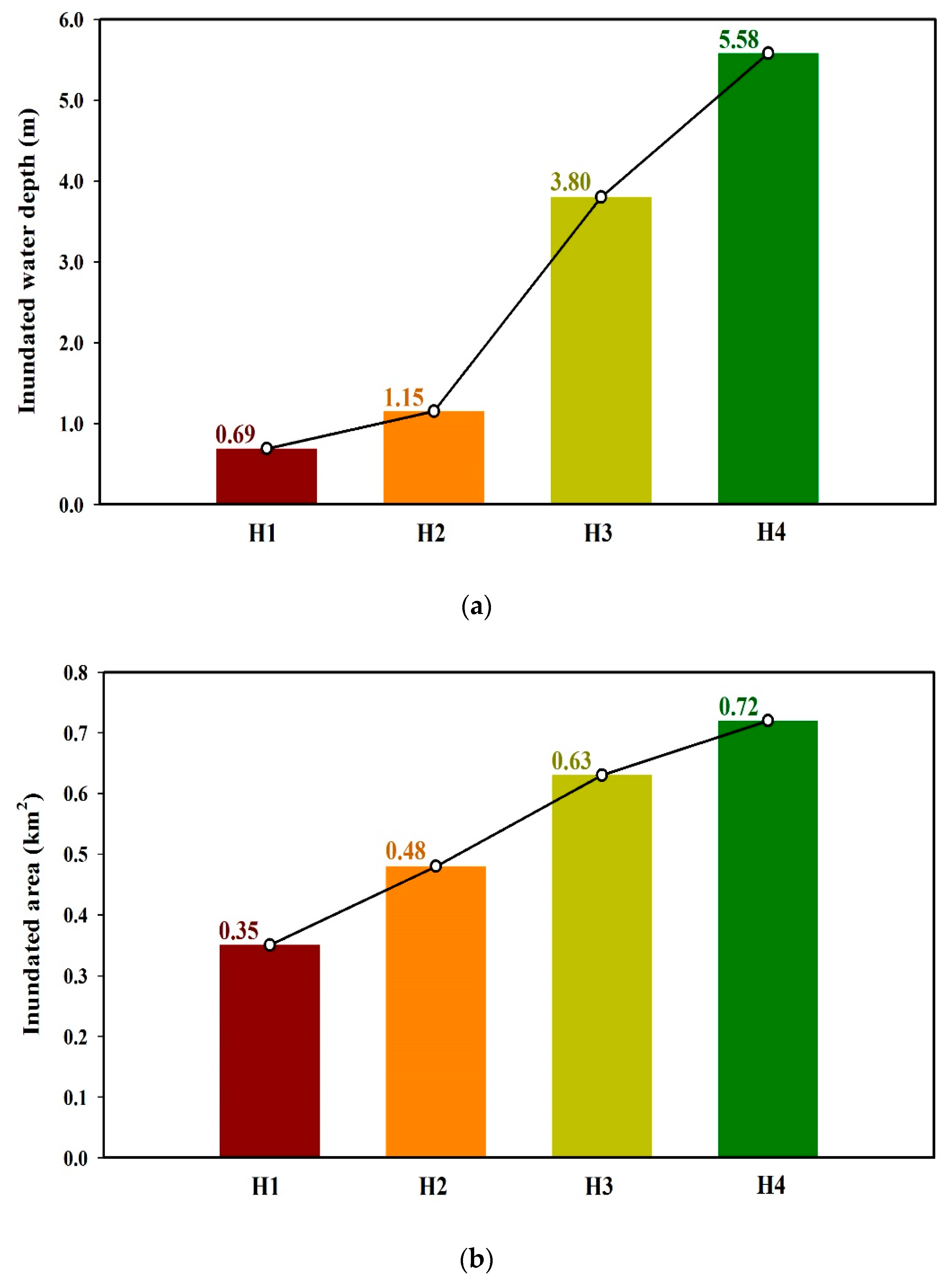
Figure 13 shows the comparison of the maximum inundated water depth and the flooded areas according to the increase in the flood inflow rate and the maximum water depths in the Gohyun river are excluded. In general, it can be seen that these characteristics increase practically linearly as the inflow rate increases. The maximum inundated water depth is calculated to be 0.69 m for H1, whereas it is calculated to be 5.58 m for H4. The difference between the two maximum inundated water depths is about eight times. The flooded area for H1 is 0.35 km², whereas that for H4 is 0.72 km². The difference between the two flooded areas is about 2.1 times. The reason the difference in the maximum inundated water depths is larger than the difference in the flooded areas is that the flood flow from the Gohyun river is propagated through the urban areas but not through the areas where the elevation is relatively higher. Therefore, the increase in the flooded area is gradual, whereas the maximum inundated water depth increases relatively rapidly owing to the continuous inflows of the flood from the Gohyun river.

4.3. Comparison of the Inundated Water Depths at the Check Points

Figure 14 shows the aspect of the changes in the inundation depths following an increase in the inflow rate at five points in urban areas: G1, G2, G3, G4 and G5 (see Figure 5). It can be seen that as the flood inflow rate increases, the maximum inundated water depth decreases. For point G1, which is closest to the Gohyun river, the maximum water depth is calculated as 0.43 m in the case of H1, 1.13 m in the case of H2, 3.67 m in the case of H3, and 5.56 m in the case of H4. Therefore, the results indicated that compared to H2, which corresponds to the period of Typhoon “Maemi”, the maximum inundated water depth is larger in the case of H3 and H4 by about 3.2 and 4.9 times, respectively, whereas it is smaller in the case of H1 by about 2.6 times. For point G5, which is located farthest from the Gohyun river, the maximum inundated water depth is calculated as 0.39 m in the case of H1, 1.15 m in the case of H2, 3.75 in the case of H3, and 5.28 m in the case of H4. Therefore, this indicates that compared to H2, the maximum inundated water depth is larger in the case of H3 and H4 by about 3.2 and 4.9 times, respectively, whereas it is smaller in the case of H1 by about 2.2 times.

Unlike the time for the start of flooding, it is estimated that the time for the realization of the maximum inundation depth increases with the increase in the inflow rates with the check point. For point G1, this time is estimated as about 23,030 s in the case of H1, 24,641 s in the case of H2, 29,669 s in the case of H3, and 30,428 s in the case of H4. Therefore, this suggests that compared to H2, the maximum inundation depth is realized later in the case of H3 and H4 by about 5028 s and 5787 s, respectively, whereas it occurs earlier in the case of H1 by about 1611 s. For point G5, the time for the achievement of the maximum inundation depth is estimated as about 27,507 s in the case of H1, 24,931 s in the case of H2, 30,605 s in the case of H3, and 30,940 s in the case of H4. Therefore, this indicates that compared to H2, the maximum inundation depth is realized later in the case of H3 and H4 by about 5674 s and 6009 s, respectively. In addition, it occurs even later in the case of H1 by about 2576 s. The reason for the increase in the time for the occurrence of the maximum inundation depth following the increase in the flood inflow rate is determined to be the fact that the floods flowing into the Gohyun river are not appropriately drained into Gohyun bay owing to the narrow river width. Moreover, the continuous flow into the urban area leads to a continuous increase in the inundated water depth in the urban area.

5. Conclusions

In the present study, a two-dimensional finite-volume model applied with the well-balanced HLLC technique was used to simulate flood inundations in the urban areas located downstream of the Gohyun river, Geoje-si, Gyeongsangnam-do. These locations sustained significant damage due to Typhoon “Maemi” in September 2003. This study verifies the applied numerical model for the simulation of the flood inundation, and the scenarios for the increases/decreases in the flood inflow rates into the Gohyun river that may occur following the typhoon are simulated, compared, and analyzed.

When the values of Manning’s roughness coefficient were distributed according to the land uses in the target area, the flooded area was estimated as 0.48 km² and the range of the inundated water depth was estimated as 0.30–1.15 m. These values were shown to coincide relatively well with the compared inundation trace data (flooded area: 0.43 km², inundation depth: 0.25–1.0 m). However, when the Manning’s roughness coefficient of 0.025 was uniformly applied, both the range of the inundated water depth and flooded area were slightly overestimated as 1.1–2.8 m and 0.55 km², respectively. Therefore, from the flood inundation simulation performed, it was determined that it is desirable to apply the Manning’s roughness coefficient values distributed appropriately according to the land uses.

According to the results of the simulation of changes in the flood inflow rate, both the flooded area and the inundated water depth increased with the flood inflow rate increase. This indicated that the design discharge capacity of the river culvert where it is in contact with the sea is significantly insufficient to drain very large floods generated during the typhoon “Maemi”. Moreover, the inland water is not smoothly drained into the sea when the tide levels become higher than the elevation of the riverbed or when massive floods occur upstream. To minimize the poor inner drainage downstream of the Gohyun river, it is necessary to increase the design discharge capacity of the existing river culvert to be discharge the flood early and also to construct the drainage pump facility for discharging the flood exceeding the design discharge capacity. The practical study related to redesigning the discharge capacity of the river culvert and the optimal drainage pumping capacity is currently underway.

References

- NIMSK. Climate Change over 100 Years on the Korean Peninsula; National Institute of Meteorological Science of Korea: Seogwipo, Korea, 2011; pp. 1–42.
- Noh, S.K.; Lee, J.S.; Kwon, K.H.; Kang, S.H. Damage Status due to Hurricane Katrina; National Institute for Disaster Prevention: New Delhi, India, 2005; Volume 7, pp. 11–22.
- National Institute for Disaster Prevention (NIDP). Field Survey Report of Damages Caused by Typhoon Maemi in 2003-Damaged by Floods, Storm Surge, Electric Power System Failure (9.12∼9.13); NIDP Field Survey Report; NIDP: New Delhi, India, 2003; pp. 1–292.
- Fukuoka, S.; Kawashim, M. Prediction of flood-induced flows in urban residential areas and damage reduction. In Floodplain Risk Management, Proceedings of the Committee of International Workshop on Floodplain Risk Management; Fukuoka, S., Ed.; A.A. Balkema: Rotterdam, The Netherlands, 1999; pp. 209–227. [Google Scholar]
- Shigeda, S.; Akiyama, J.; Ura, M. Numerical Simulation of Flood Propagation in a Floodplain with Structures. J. Hydrosci. Hydraul. Eng. 2002, 20, 117–129. [Google Scholar]
- Shigeda, S.; Akiyama, J. Numerical and Experimental Study on Two-Dimensional Flood Flows with and without Structures. J. Hydraul. Eng. 2003, 129, 817–821. [Google Scholar] [CrossRef]
- Soares-Frazao, S.; Noel, B.; Zech, Y. Experiments of dam-break flow in the presence of obstacles. In Proceedings of the River Flow 2004 Conference, Naples, Italy, 23–25 June 2004; Volume 2, pp. 911–918. [Google Scholar]
- Mignot, E.; Paquier, A.; Riviere, N. How a 2-D code can simulate urban flood simulation. In Proceedings of the River Flow 2004 Conference, Naples, Italy, 23–25 June 2004; Volume 2, pp. 1031–1040. [Google Scholar]
- Mignot, E.; Paquier, A.; Haider, S. Modeling floods in a dense urban area using 2D shallow water equations. J. Hydrol. 2006, 327, 186–199. [Google Scholar] [CrossRef] [Green Version]
- Neal, J.C.; Bates, P.D.; Fewrell, T.J.; Hunter, N.M.; Wilson, M.D.; Horritt, M.S. Distributed whole city water level measurements from the Carlisle 2005 urban flood event and comparison with hydraulic model simulations. J. Hydrol. 2009, 368, 42–55. [Google Scholar] [CrossRef]
- Begnudelli, L. Sanders BF Unstructured grid finite volume algorithm for shallow-water flow and transport with wetting and drying. J. Hydraul. Eng. 2006, 132, 1777–1795. [Google Scholar] [CrossRef]
- Humberto, A.; Gallegos, A.; Jochen, E.; Schubert, E.; Sanders, B.F. Two-dimensional, high-resolution modeling of urban dam-break flooding; A case study of Baldwin Hills, California. Adv. Water Resour. 2009, 32, 1323–1335. [Google Scholar]
- Jeong, W.C.; Cho, Y.S.; Lee, J.W. A Numerical Study on Characteristics of Flood Wave Passing through Urban Areas (1): Development and Verification of a Numerical Model. J. Korean Soc. Hazard Mitig. 2009, 9, 89–97. [Google Scholar]
- Jeong, W.C.; Cho, Y.S.; Lee, J.W. A Numerical Study on Characteristics of Flood Wave Passing through Urban Areas (2): Application and Analysis. J. Korean Soc. Hazard Mitig. 2010, 10, 65–72. [Google Scholar]
- Andisio, C.; Turconi, L. Urban Floods: A Case Study in the Savigliano Area (North-Western Italy). Nat. Hazards Earth Syst. Sci. 2011, 11, 2951–2964. [Google Scholar] [CrossRef]
- Gallien, T.W.; Sanders, B.F.; Flick, R.E. Urban coastal flood prediction: Integrating wave overtopping, flood defenses and drainage. Coast. Eng. 2014, 91, 18–28. [Google Scholar] [CrossRef]
- LeRoy, S.; Pedreros, R.; André, C.; Paris, F.; Lecacheux, S.; Marche, F.; Vinchon, C. Coastal flooding of urban areas by overtopping: Dynamic modelling application to the Johanna storm in Gâvres (France). Nat. Hazards Earth Syst. Sci. 2015, 15, 2497–2510. [Google Scholar] [CrossRef]
- Vojinovic, Z.; Seyoum, S.; Salum, M.H.; Price, R.K.; Fikri, A.K.; Abebe, Y. Modelling floods in urban areas and representation of buildings with a method based on adjusted conveyance and storage characteristics. J. Hydroinform. 2013, 15, 1150–1168. [Google Scholar] [CrossRef]
- Roccati, A.; Lucino, F.; Turconi, L.; Piana, P.; Watkins, C.; Faccini, F. Historical geomorphological research of a ligurian coastal floodplain (Italy) and its value for Management of flood risk and environmental sustainability. Sustainability 2018, 10, 3727. [Google Scholar] [CrossRef]
- Paliaga, G.; Faccini, F.; Lucino FTurconi, L.; Bobrowsky, P. Geomorphic processes and risk related to a large landslide dam in a highly urbanized Mediterranean catchment (Genova, Italy). Geomorphology 2019, 327, 48–61. [Google Scholar] [CrossRef]
- Jeong, W.C.; Kim, K.H. A Study on Inundation Simulation in Coastal Urban Areas Using a Two-Dimensional Numerical Model. J. Water Resour. Assoc. 2011, 44, 601–617. [Google Scholar] [CrossRef] [Green Version]
- Jeong, W.C. A Study on simulation of flood inundation in a coastal urban area using a two-dimensional well-balanced finite volume model. Nat. Hazards 2015, 77, 337–357. [Google Scholar] [CrossRef]
- Toro, E.F. Shock-Capturing Methods for Free-Surface Shallow Flows; Wiley: New York, NY, USA, 2001; pp. 1–309. [Google Scholar]
- Billet, S.J.; Toro, E.F. On WAF-type schemes for multi-dimensional hyperbolic conservation laws. J. Comput. Phys. 1997, 130, 1–24. [Google Scholar] [CrossRef]
- Harten ALax, P.; van Leer, A. On upstream differencing and Godunov-type scheme for hyperbolic conservation laws. Soc. Ind. Appl. Math. Rev. 1983, 25, 35–61. [Google Scholar] [CrossRef]
- Kim, D.H.; Cho, Y.S.; Kim, H.J. Well-balanced scheme between flux and source terms for computation of shallow-water equations over irregular bathymetry. J. Eng. Mech. 2008, 134, 277–290. [Google Scholar] [CrossRef]
- Perthame, B.; Simeoni, C. A kinetic scheme for the Saint-Venant extended Kalman Filter for data assimiliation in oceanography. Calcolo 2001, 38, 201–231. [Google Scholar] [CrossRef]
- LeVeque, R.L.; George, D.L. High-resolution finite volume methods for the shallow water equations with bathymetry and dry states. In Advances in Coastal and Ocean Engineering, Proceedings of the Third International Workshop on long-Wave Runup Model, Wrigley Marine Science Center Catalina Island, California, 17–18 June 2004; Advances in Coastal and Ocean Engineering, Catalina, 2004; Cornell University: Ithaca, NY, USA, 1999; Volume 10, pp. 43–73. [Google Scholar]
- Loukili, Y.; Soulaïmani, A. Numerical Tracking of Shallow Water Waves by the Unstructured Finite Volume WAF Approximation. Int. J. Comput. Methods Eng. Sci. Mech. 2007, 8, 1–14. [Google Scholar] [CrossRef]
- Honnorat, M. Assimilation de Données Lagrangiennes pour la Simulation Numérique en Hydraulique Fluvial. Ph.D. Thesis, Institute National Polytechnique de Grenoble, Grenoble, France, 2007. [Google Scholar]
- Korea Meteorological Administration (KMA). Available online: http://www.weather.go.kr/weather/climate/ (accessed on 30 September 2018).
- U.S. Army Corps of Engineering. HEC-HMS User’s Manual Version 4.2; U.S. Army Corps of Engineering: Washington, DC, USA, 2016.
- Geoje City Government. Internal Report of Comprehensive Planning System for Flood Damage Mitigation; Geoje City Government: Geoje, Korea, 2003; pp. 1–1320.
- Halwatura, D.; Najim, M. Application of the HEC-HMS model for runoff simulation in a tropical catchment. Environ. Model. Softw. 2005, 46, 155–162. [Google Scholar] [CrossRef]
- Jin, H.; Liang, R.; Wang, Y.; Tumula, P. Flood-runoff in semi-arid and sub-humid regions, a case study: A simulation of jianghe watershed in northern China. Water 2015, 7, 5155–5172. [Google Scholar] [CrossRef]
- Feldman, A. Hydrologic Modeling System HEC-HMS technical reference manual. In US Army Corps of Engineers; Hydrologic Engineering Center: Davis, CA, USA, 2000. [Google Scholar]
- Schubert, J.E.; Sanders, B.F. Building treatments for urban flood inundation models and implications for predictive skill an modeling efficiency. Adv. Water Resour. 2012, 41, 59–64. [Google Scholar] [CrossRef]
- Schubert, J.E.; Sanders, B.F.; Smith, M.J.; Wright, N.G. Unstructured mesh generation and land cover-based resistance for hydrodynamic modeling of urban flooding. Adv. Water Resour. 2008, 31, 1603–1621. [Google Scholar] [CrossRef]
- Liang, D.; Falconer, R.A.; Lin, B. Coupling surface and subsurface flows in a depth averaged flood wave model. J. Hydrol. 2007, 337, 147–158. [Google Scholar] [CrossRef]
- Yamashita, K.; Suppasri, A.; Oishi, Y.; Imamura, F. Development of a Tsunami Inundation Analysis Model for Urban Areas Using a Porous Body Model. Geosciences 2018, 8, 12. [Google Scholar] [CrossRef]
- Baba, T.; Takahashi, N.; Kaneda, Y.; Inazawa, Y.; Kikkojin, M. Tsunami Inundation Modeling of the 2011 Tohoku Earthquake Using Three-Dimensional Building Data for Sendai, Miyagi Prefecture, Japan. In Tsunami Events and Lessons Learned: Environmental and Societal Significance; Kontar, Y., Santiago-Fandiño, V., Takahashi, T., Eds.; Springer: Dordrecht, The Netherlands, 2014; pp. 89–98. [Google Scholar]
- National Geographic Information Institute (NGII). Available online: http://map.ngii.go.kr/ (accessed on 1 October 2018).
- Lee, J.S. Fluid Mechanics for Civil Engineers; Goomi Press: Seoul, Korea, 2011; pp. 1–350. [Google Scholar]
- Engman, E.T. Roughness Coefficients for Routing Surface Runoff. J. Irrig. Drain. Eng. 1986, 112, 39–53. [Google Scholar] [CrossRef]
Figure 1.
Triangular and quadrilateral cells in a two-dimensional unstructured grid system [22].
Figure 2.
Schematic illustration of Harten–Lax–Van Leer contact (HLLC) flux approximation.
Figure 3.
Satellite image of a coastal urban area in the Gohyun river basin and target area (unit: meter).
Figure 4.
Temporal distributions of the rainfall (a) and flood inflow (b).
Figure 5.
Unstructured grid system and locations of the five check points.
Figure 6.
Distribution of Manning’s roughness coefficients with land use.
Figure 7.
Temporal variation in the tidal level imposed on the outflow boundary.
Figure 8.
Comparison of spatial distributions of inundated water depth with time for Case 1 and 2.
Figure 9.
Comparison between the surveyed inundation trace and the simulated inundation distribution for Case 1 and 2 (Red line represents the boundary of flooded area).
Figure 10.
Temporal variation of tide levels during typhoon “Maemi”.
Figure 11.
Flood hydrographs for the four scenarios.
Figure 12.
Spatial distribution of the inundated water depth in the four scenarios of the flood inflow rate.
Figure 13.
Comparison of (a) maximum inundated water depths and (b) inundated area in the four scenarios of the flood inflow rate.
Figure 14.
Temporal variation in the inundated water depth at the five check points in the four scenarios of the flood inflow rate.