Numerical Study of the Hydrodynamics of Waves and Currents and Their Effects in Pier Scouring

Abstract

The scour around cylindrical piles due to codirectional and opposite waves and currents is studied with Reynolds Averaged Navier–Stokes (RANS) equations via REEF3D numeric modeling. First, a calibration process was made through a comparison with the experimental data available in the literature. Subsequently, not only the hydrodynamics, but also the expected scour for a set of scenarios, which were defined by the relative velocity of the current ($U_{CW}$), were studied numerically. The results obtained show that the hydrodynamics around the pile for codirectional or opposite waves and currents not have significant differences when analyzed in terms of their velocities, vorticities and mean shear stresses, since the currents proved to be more relevant compared to the net flow. The equilibrium scour, estimated by the extrapolation of the numerical data with the equation by Sheppard, enabled us to estimate values close to those described in the literature. From this extrapolation, it was verified that the dimensionless scour would be less when the waves and currents are from opposite directions. The $U_{CW}$ parameter is an indicator used to adequately measure the interactions between the currents and waves under conditions of codirectional flow. Nevertheless, it is recommended to modify this parameter for currents and waves in opposite directions, and an equation is proposed for this case.

1. Introduction

The hydrodynamics of the coastal environment usually correspond to the result of the interaction of several force, such as waves, tides, and winds, that act at different spatial and temporal scales, thereby modulating circulation. Meanwhile, rivers run mainly due to the gravitational action that moves the waters resulting from snowmelt or rain, which flow into the alluvial channel that transports to the ocean by runoff. The convergence of coastal and fluvial environments is known as an estuary zone, and the resulting currents correspond to a complex interaction between tides, waves, winds, and river flow.

The hydrodynamics of environments where waves and currents interact have been previously studied by various authors both co-directionally [1,2,3] and perpendicularly [4,5,6].

The research developed by Umeyama [1,2,3], sought to analyze the behavior of Reynolds stress and velocity vertical distributions [1], the changes induced by the combined wave currents over the turbulent flow structures [2], and the surface elevation and particle velocities [3].

In the case of waves orthogonal to currents, the experimental research developed by Feraci et al. [4], Lim and Madsen [5] and Feraci et al. [6] allows us to understand the effects of joint action on the behavior of the resulting velocity of the fluid. For example, Feraci et al. [4] experimentally demonstrated the joint action of orthogonal waves and currents, which speeds up the evolution process of a sandpit. Lim and Madsen [5] analyzed, via an experimental study the effects of the roughness in an experimental study on the velocity distribution in a wave-current interaction. A complete statistical analysis of the near bed velocity behavior due to waves and a current acting perpendicularly was developed by Feraci et al. [6]. They concluded that the probability distribution of near-bed velocity follows a Gaussian distribution in a flow field generated by a current alone. In the presence of waves, the distribution changes and another peak over a Gaussian distribution appears.

However, all the studies in the previous paragraphs do not include any type of obstruction to the flow, which generates additional modifications to the hydrodynamic characteristics of the flow field.

It is well known that when placing a circular pile in an environment that has a specific current (that can be produced by waves/tides, river flow, or both), a hydrodynamic modification will be produced around it and, therefore, vortexes will be produced (a horseshoe vortex and vortex shedding), which are the main elements responsible for the scour around the pile.

Through time, different authors have studied pile scour due to a uniform flow. Among these authors it is worth mentioning Hjorth [7], Melville [8], Ettema [9], Chiew and Melville [10], Melville and Chiew [11], Oliveto and Hager [12], Link et al. [13], Diab et al. [14], and Link et al. [15], who focused their interests mainly on the scour around bridge piles. When it comes to scour by waves, the number of studies is limited. On this subject, the authors of this paper consider the contributions of Sumer et al. [16], Sumer et al. [17] and Sumer and Fredsøe [18] to be fundamental to our understanding of multiple hydrodynamic processes responsible for the movement of sediments near the pile.

Experimental studies on the scour around piles under a flow associated with the combined action of waves and currents have been carried out by different authors [19,20,21,22,23,24,25,26], who have contributed, through their laboratory tests, to our understanding of the scour phenomenon in this type of environments. The following is a brief bibliographic description.

Eadie and Hernich [19] studied a physical model with the purpose of evaluating the effects that the combined action of two co-directional forces, waves (random) and currents, have over the scour around cylindric piles. The main results of Eadie and Hernich [19] indicate that the scour process due to waves and currents together is faster and reaches higher equilibrium compared to currents acting alone. Similar results were determined by Kawata and Tsichiya [20], who characterized the scour process for clear-water and live-beds in a similar manner to Eadie and Hernich [19].

Raaijmakers and Rudolph [15] studied the temporal dependency of the scour around a pile due to the combined action of waves and currents with the purpose of analyzing the equilibrium scour, the temporal scales needed to reach such depths and the backfilling process. As part of their results, Raaijmakers and Rudolph [21] propose an equation to determine the scour as a function of time and additionally concluded that the equilibrium scour is of a higher magnitude in cases of currents acting alone compared to the conditions reached for the combined action of waves and currents. The equilibrium scour equation as a function of time, presented by Raaijmakers and Rudolph [21], was validated through the comparison of field data, as presented by Rudolph et al. [22].

Zanke et al. [23], through an analysis of data gathered by other authors, proposed a unified equation to determine the scour depth due to the actions of waves and currents, through the incorporation of a transition function ($x_{rel}$) defined by the effective scour ($x_{eff}$). Similarly, Ong et al. [24] developed a stochastic method by which the maximum equilibrium scour could be determined in piles exposed to long-crested and short-crested nonlinear random waves plus a current. They validated their approach by comparison with the experimental data provided by Sumer and Fredsøe [25].

The contribution carried out by Sumer and Fredsøe [25] to understand the process of scour is significant, since through its dimensional analysis, their model is able to represent the dimensionless scour ($S$) over the pile diameter ($D$) as a function of relative flow velocity ($U_{cw}$), as defined by Equation (1), where $U_c$ corresponds to the undisturbed current velocity at the transverse distance $z=D/2$ and $U_m$ is the maximum value of the undisturbed orbital velocity at sea bottom just above the wave’s boundary layer:

$$U_{cw}=\frac{U_c}{U_c+U_m}.$$

(1)

Evidently, the relative flow velocity will have values close to zero when the environment is dominated by waves, but it will approach one if currents are the main flow mechanism.

The main conclusions presented by Sumer and Fredsøe [25] indicate that in a wave environment, the scour increases significantly in the presence of a current, even if the current is mild. This current, is mainly associated with a strong horseshoe vortex in front of the pile, even in the case of a mild vortex. In addition, the current apparently dominates the pile’s scour when $U_{cw}\ge 0.7$; the scour approaches this value due to the current acting alone.

Even though the articles mentioned above have studied the scour around cylindrical piles due to the combined action of waves and currents, they considered forcing to act co-directionally. Qi and Gao [26], in their experimental work, studied the scour around cylindrical piles under the combined action of co-directional and opposite waves and currents, for different pile diameters, waves conditions and currents. The main conclusion they reached was that the scour in the combined flows of waves and currents is a nonlinear process, and the time required to reach scour equilibrium is much lower than that required for waves or currents acting independently. Additionally, Qi and Gao [26] mentioned that the maximum flow velocity in waves and co-directional currents is much higher than that in waves and currents from opposite directions, thereby affecting the maximum scour magnitude, which is lower in opposite flows.

While there is a number (albeit limited) of experimental articles related to the study of scour caused by combined waves and currents, investigations based on numerical models are even more scarce. It is only possible to find simulations of scour acting separately around piles due to currents or oscillatory flows. A literature review on this subject is available on Quezada et al. [27].

The application of Reynolds-averaged Navier–Stokes equations (RANS) in simulated environments, in which waves and currents coexist, has been demonstrated by several authors [28,29,30], who nonetheless fail to include the vertical pile in the flow. Ahmad et al. [31] recently developed a numerical study based on the REEF3D model in order to study scour on a horizontal pile (pipeline) caused by combined waves and currents. This study is relevant to the research presented in this article, since the same numerical model used by Ahmad et al. [31] was applied.

Based on the above, the main objective of this article is to study, through numerical models, scour’s hydrodynamics around cylindrical piles where waves and currents coexist, both co-directional and opposite to the wave direction as well.

2. Materials and Methods

2.1. Numerical Model: REEF3D

The numerical modelling developed in this research was conducted using the numerical model known as REEF3D [32,33], which is a computational fluid dynamic (CFD) tool used to solve Reynolds-averaged Navier–Stokes equations (RANS). This tool is able to simulate hydraulic, coastal, and estuarine phenomena for both compressible and incompressible fluids.

The REEF3D model provides a three-dimensional solution for governing equations composed of Equation (2), which corresponds to the continuity of an incompressible flow, and Equation (3), which is the momentum conservation.

$$\frac{\partial u_i}{\partial x_i}=0$$

(2)

$$\frac{\partial u_i}{\partial t}+u_j\frac{\partial u_i}{\partial x_j}=-\frac{1}{\rho }\frac{\partial p}{\partial x_i}+\frac{\partial }{\partial x_j}\left[\left(\upsilon +{\upsilon }_T\right)\frac{\partial u_i}{\partial x_j}\right]+g_i,$$

(3)

where i, j = 1,2,3, $u_i$ is the mean velocity vectoral component, $x_i$ is the spatial vectoral component, $t$ is time, $\rho$ is water density, $p$ is pressure, $\upsilon$ is kinematic viscosity, ${\upsilon }_T$ is kinematic eddy viscosity, and $g$ is gravity.

The turbulence closure model used was the well-known $k-\omega$ model [34], in which ${\upsilon }_T$ is defined according to Equation (4), and both the turbulent kinetic energy ($k$) and the kinetic energy for the specific turbulent dissipation per unit of turbulence ($\omega$) are determined with a transport equation, according to Equations (5) and (6), respectively. The constant values in $k-\omega$ were taken according to ${\beta }_k$ = 9/100, $\alpha$ = 5/9, $\beta$ = 3/40, ${\sigma }_{\omega }$ = 1/2, and ${\sigma }_k$ = 1; and $P_k$ is the turbulent production rate defined by Equation (7).

$${\upsilon }_T=\frac{k}{\omega }$$

(4)

$$\frac{\partial k}{\partial t}+u_j\frac{\partial k}{\partial x_j}=\frac{\partial }{\partial x_j}\left[\left(\upsilon +\frac{{\upsilon }_T}{{\sigma }_k}\right)\frac{\partial k}{\partial x_j}\right]+P_k-{\beta }_{k}k\omega$$

(5)

$$\frac{\partial \omega }{\partial t}+u_j\frac{\partial \omega }{\partial x_j}=\frac{\partial }{\partial x_j}\left[\left(\upsilon +\frac{{\upsilon }_T}{{\sigma }_{\omega }}\right)\frac{\partial \omega }{\partial x_j}\right]+\frac{\omega }{k}\alpha P_k-\beta {\omega }^2$$

(6)

$$P_k={\upsilon }_T\frac{\partial u_i}{\partial x_j}\left[\frac{\partial u_i}{\partial x_j}+\frac{\partial u_j}{\partial x_i}\right].$$

(7)

To solve the flow around complex structures, the ghost-cell method [35,36] was applied to impose the boundary conditions when a pile is included in the numerical domain. This approach uses fictional cells that are incorporated in the domain (specifically on the obstacles) and corresponds to a particular case of the immersed boundary method [37].

The numerical treatment of the governing equations was based on the second order of the Runge–Kutta method for temporal discretization. Meanwhile, the convective terms were solved by the applied weight essentially non-oscillatory (WENO) scheme [38]. The velocities and pressures were determined under a staggered grid, using the Semi-Implicit Method for Pressure Linked Equations (SIMPLE) [39].

The model configuration to represent waves in the numerical domain was adopted similar to the method presented by Ahmad et al. [31], using a Dirichlet boundary condition and the second-order Stokes waves theory [40]. We defined the surface elevation ($\eta$) and the incident velocity ($u,w$) according to Equations (8) and (9), respectively.

$$\eta \left(x,z,t\right)=\frac{H}{2}\cos \vartheta +\frac{H^{2}K}{16}\frac{\cos h\left(Kh\right)}{\sin h^3\left(Kh\right)}\left(2+\cos h\left(2Kh\right)\right)\cos \left(2\vartheta \right)$$

(8)

$$u\left(x,z,t\right)=\frac{\partial \mathsf{\Phi }}{\partial \mathrm{x}},w\left(x,z,t\right)=-\frac{\partial \mathsf{\Phi }}{\partial \mathrm{z}}$$

(9)

$$\Phi \left(x,z,t\right)=\frac{Hg}{2\varpi }\frac{\cos h\left[K\left(h+z\right)\right]}{\cos h\left(Kh\right)}\sin \vartheta +\frac{3}{32}{H}^2\varpi \frac{\cos h\left[2K\left(h+z\right)\right]}{\sin h^2\left(Kh\right)}\sin \left(2\vartheta \right),$$

(10)

where $H$ is wave height, $K$ is the wave number, $h$ is the water depth, $\vartheta$ is the wave phase, $\varpi$ is the angular frequency, and $\Phi$ is the velocity potential.

In order to avoid the wave reflection, active wave absorption (AWA), was used in the outlet according to the method described by Schäffer and Klopman [41]. In this methodology, the waves that reach the outlet cancel out the reflected waves, prescribing the velocity as in [31]:

$$u_0=-\sqrt{\frac{g}{h}}{\eta }_r$$

(11)

$${\eta }_r={\eta }_m-h,$$

(12)

where ${\eta }_r$ is the reflected wave amplitude and ${\eta }_m$ is the actual elevation of the free surface.

Complementary information on the numerical model´s hydrodynamic configuration is shown in

Table 1. Complementary information for the REEF3D hydrodynamic simulation.

Configuration	Definition
Boundary condition	Non-slip for velocities
	Non-slip for$k$ and $\omega$
	Logarithmic profile for inlet
	Fix pressure at inlet
	Zero-gradient outflow
	Active wave absorption at outlet (waves)
Initialization	Potential flow for velocities
	Hydrostatic for pressure

.

In order to ascertain the sediment transport and changes in the bed, both the bed load and the suspended load were considered, for the morphodynamics evolution, the equation for the conservation of sediment initially proposed by Exner [42] and later generalized by Paola and Voller [43], was used.

The bed load sediment transport was computed by using the Meyer–Peter formula [44] according to Equation (13), where $q_b^{*}$ is the dimensionless bed load, ${\tau }^{*}$ is the dimensionless shear stress on the bed computed by Equation (14), ${\tau }_c^{*}$ is the dimensionless critical shear stress defined according to the Equation (15), $\tau$ is the bed shear stress, ${\tau }_c$ is the critical bed shear stress, ${\rho }_s$ the sediment density, and $d$ is the sediment diameter. The real magnitude of the bed load ($q_b$) can be obtained from Equation (16).

$$q_b^{*}=8{\left({\tau }^{*}-{\tau }_c^{*}\right)}^{\raisebox{1ex}{$3$}\!\left/ \!\raisebox{-1ex}{$2$}\right.}$$

(13)

$${\tau }^{*}=\frac{\tau }{\left({\rho }_s-\rho \right)gd}$$

(14)

$${\tau }_c^{*}=\frac{{\tau }_c}{\left({\rho }_s-\rho \right)gd}$$

(15)

$$q_b^{*}=\frac{q_b}{\sqrt{\frac{\left({\rho }_s-\rho \right)g{d}^3}{\rho }}}.$$

(16)

The suspended load was computed using the advection diffusion equation shown in Equation (17), where $c$ is the suspended load concentration, and $w_s$ is the fall velocity of the sediment. To solve Equation (17) two boundary conditions were applied. The first is the zero vertical flux on the surface and the second is the bed load concentration ($c_b$) according to Van Rijn [45], defined by Equation (18), where $\mathsf{{\rm Y}}$ is the relative bed shear stress defined by Equation (19), and $D_{*}$ is the particle parameter computed according to Equation (20).

$$\frac{\partial c}{\partial t}+u_j\frac{\partial c}{\partial x_j}+w_s\frac{\partial c}{\partial z}=\frac{\partial }{\partial x_j}\left({\upsilon }_T\frac{\partial c}{\partial x_j}\right)$$

(17)

$$c_b=0.015\frac{d}{a}\left(\frac{{\mathsf{{\rm Y}}}^{1.5}}{D_{*}^{0.3}}\right)$$

(18)

$$\mathsf{{\rm Y}}=\frac{\left(\tau -{\tau }_c\right)}{{\tau }_c}$$

(19)

$$D_{*}=d{\left[\frac{\left(s-1\right)g}{{\upsilon }^2}\right]}^{\raisebox{1ex}{$1$}\!\left/ \!\raisebox{-1ex}{$3$}\right.}$$

(20)

In Equation (18), $a$ is the reference level for computing the suspended load that has been determined according to the methodology proposed by Rouse [46].

The critical bed shear stress was defined according to Shields [47] and parameterized according to Yalin [48], including the slope correction proposed by Dey [49] and, in addition, applying the incipient transport relaxation factor extensively described by Quezada et al. [27].

The morpho-dynamic evolution was determined by the sediment volume conservation equation described in Equation (21), where $z_b$ is the bed elevation, and $q_{b,x}$ and $q_{b,y}$ are the sediment transport for the bed load in the $x$ and $y$ directions, respectively. $E$ is the sediment entrainment rate from the bed load to the suspended-load, and $D$ is the sediment deposition rate from the suspended load onto the bed.

$$\frac{\partial z_b}{\partial t}+\frac{1}{\left(1-n\right)}\left[\frac{\partial q_{b,x}}{\partial x}+\frac{\partial q_{b,y}}{\partial y}\right]+E-D=0.$$

(21)

The difference between $E$ and $D$ is defined by REEF3D according to Wu et al. [50]. Meanwhile, a more extensive description of the estimation of $q_{b,x}$ and $q_{b,y}$ can be found in Quezada et al. [27].

In order to develop a numerical study of the present investigation, the model was developed as indicated in

Table 2. Summary of the REEF3D model configuration applied to each simulated cases.

Case	$\mathit{L}$ (m)	$\mathit{W}$ (m)	${\mathit{h}}_{\mathit{t}}\left(\mathbf{m}\right)$	$\mathbf{\Delta }{\mathit{x}}_{\mathit{i}}\left(\mathbf{m}\right)$	N° Cells	${\mathit{t}}_{\mathit{t}\mathit{e}\mathit{s}\mathit{t}}\left(\mathbf{min}\right)$
W1	24.00	0.70	1.00	0.01	16,768,400	5.00
W2	24.00	0.70	1.00	0.01	16,768,400	5.00
W3	24.00	0.70	1.00	0.01	16,768,400	5.00
WC1	24.00	0.70	1.00	0.01	16,768,400	5.00
WC2	24.00	0.70	1.00	0.01	16,768,400	5.00
WC3	24.00	0.70	1.00	0.01	16,768,400	5.00
C01	24.00	1.00	1.00	0.01	23,968,400	7.00
C02	24.00	1.00	1.00	0.01	23,968,400	7.00
C03	24.00	1.00	1.00	0.01	23,968,400	7.00
C04	24.00	24.00	1.00	0.01	575,968,400	1.00
E01	24.00	1.00	1.00	0.01	23,968,400	30.00
E02	24.00	1.00	1.00	0.01	23,968,400	30.00
E03	24.00	1.00	1.00	0.01	23,968,400	30.00
E04	24.00	1.00	1.00	0.01	23,968,400	30.00
E05	24.00	1.00	1.00	0.01	23,968,400	30.00
E06	24.00	1.00	1.00	0.01	23,968,400	30.00
E07	24.00	1.00	1.00	0.01	23,968,400	30.00
E08	24.00	1.00	1.00	0.01	23,968,400	30.00

∆x_i is the dimension for the x, y, and z axis, due to the model using regular element definitions.

, where $L$ is the flume length, $W$ is the width, $h_t$ is the height, and $\Delta x_i$ is the cell dimension used in the model; N° Cells is the total number of elements comprising the numerical domain, and $t_{test}$ is the simulation time of the numerical model. The W (W1 to W3) and WC series (WC1 to WC3) correspond to a hydrodynamic calibration stage for waves acting alone and waves plus current, respectively, without a pile placed on the flume. Detailed information can be found in

Table 3. Hydrodynamic calibration of waves and currents coexisting without a pile.

Case	$\mathit{h}$ (m)	$\mathit{H}$ (cm)	$\mathit{T}$ (s)	${\mathit{U}}_{\mathit{C}}(\mathbf{cm}/\mathbf{s})$
W1	0.30	1.03	1.00	0.00
W2	0.30	2.34	1.00	0.00
W3	0.30	3.61	1.00	0.00
WC1	0.30	0.91	1.00	8.00
WC2	0.30	2.02	1.00	8.00
WC3	0.30	3.09	1.00	8.00

.

Series C (C01 to C04) corresponds to a hydrodynamic stage for waves plus current with a pile. Detailed information for each test can be found in

Table 4. Hydrodynamic calibration of waves and currents coexisting with pile.

Case	$\mathit{h}$ (m)	$\mathit{D}$ (m)	$\mathit{H}$ (cm)	$\mathit{T}$ (s)	${\mathit{U}}_{\mathit{C}}(\mathbf{m}/\mathbf{s})$	Direction
C01	0.50	0.20	2.60	1.40	0.23	Codirectional
C02	0.50	0.20	5.20	1.40	0.23	Codirectional
C03	0.50	0.20	8.50	1.40	0.23	Codirectional
C04	0.50	0.20	4.00	1.25	0.25	Perpendicular

. Finally, series E (E01 to E08) corresponds to the simulated cases for hydrodynamic analysis due to the combined action of waves and currents; their detailed information can be found in

Table 5. Simulated cases for the analysis of hydrodynamics due to the combined action of waves and currents.

Case	$\mathit{h}$ (m)	$\mathit{D}$ (m)	$\mathit{H}$ (m)	$\mathit{T}$ (s)	${\mathit{U}}_{\mathit{C}}(\mathbf{m}/\mathbf{s})$	${\mathit{U}}_{\mathit{m}}(\mathbf{m}/\mathbf{s})$	${\mathit{U}}_{\mathit{c}\mathit{w}}$	$\mathit{K}\mathit{C}$	Direction
E01	0.50	0.20	0.085	1.40	0.23	0.12	0.65	0.86	Codirectional
E02	0.50	0.20	0.085	1.40	0.23	0.12	0.65	0.86	Opposite
E03	0.50	0.20	0.129	1.40	0.22	0.19	0.54	1.31	Codirectional
E04	0.50	0.20	0.129	1.40	0.22	0.19	0.54	1.31	Opposite
E05	0.50	0.20	0.150	2.00	0.24	0.28	0.47	2.76	Codirectional
E06	0.50	0.20	0.150	2.00	0.24	0.28	0.47	2.76	Opposite
E07	0.50	0.20	0.150	3.00	0.10	0.31	0.25	4.61	Codirectional
E08	0.50	0.20	0.150	3.00	0.10	0.31	0.25	4.61	Opposite

.

The following sections provide more exstensive information on the simulated scenarios and the data processing used.

2.2. Hydrodynamics Calibration Test

Prior to executing a numerical simulation of scour due to the combined waves and currents around a circular pile, the process of hydrodynamically calibrating the model REEF3D was conducted by comparing the numerical results with the experimental results obtained by other authors.

The calibration process was carried out in two phases. The first phase to verified the numerical model’s capacity to represent a flow of waves and currents combined, without the pile in the flume, while the second calibration phase included the presence of a vertical pile in the center of the flume.

In Table 3, cases executed in the hydrodynamic calibration process without considering the pile are described. The experimental information for each of the cases was obtained from Umeyama [3], and these data correspond to the unevenness data for the water surface and the vertical profiles of flow horizontal velocity for different times steps, both for the flow caused only by the actions of waves (case W1 to W3) and by waves and currents (cases WC1 to WC3).

The variables in Table 3 are defined as follows: h is water depth, H is wave height, T is the wave periodic time, and $U_C$ is the undisturbed current velocity defined according to Sumer and Fredsøe [25].

In order to compare the results obtained by the numerical model and those provided by Umeyama’s [3] experimental work, a virtual sensor was established in the middle of the numerical domain, from which the vertical distribution (from the total velocity), and the surface elevation were extracted. The simulation time for all scenarios of the situation without pile (W1 to WC3) was five minutes (300 waves).

Simulated cases for the hydrodynamic calibration of the numerical model, including one pile in a flow due to waves and the combined action of currents, are summarized in Table 4, which considers simulated cases for codirectional (C01 to C03) and perpendicular (C04) waves and currents.

The numerical results obtained by the simulation for cases C01 to C03 (codirectional) contrasted with the experimental data provided by Qi and Gao [26], where the flow velocity was the comparison variable. For the case of the perpendicular waves and currents (C04), the experimental information provided by Miles et al. [51] was used to verify the numerical results, where the contrasted variable was the average vertical profile of the total flow velocity.

The comparison of the numerical and experimental data obtained by Qi and Gao [26] (C01 to C03) was carried out by obtaining the time series of the total velocity in a virtual monitoring station located at the horizontal 20D and 1D relative to the bed. The total time of the simulation was seven minutes (300 waves).

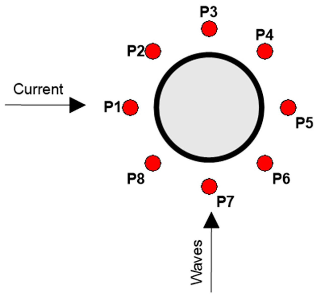
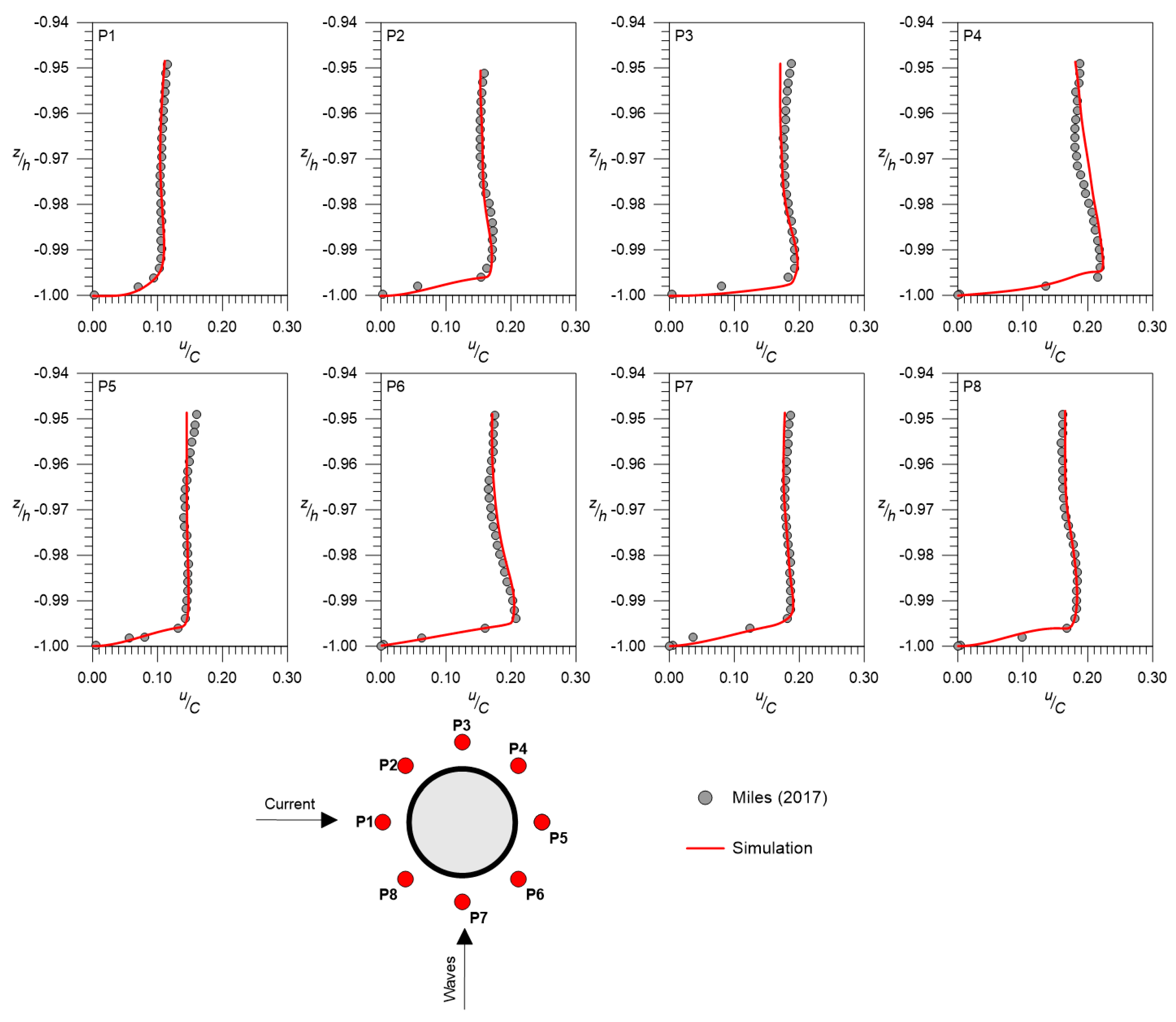
For case C04, the comparison of numerical and experimental data published by Miles et al. [51] was conducted via the vertical distribution of the longitudinal velocity averaged in eight points around the pile, which were denominated P1 to P8 and distributed as shown in Figure 1. The monitoring stations were located 0.75$D$ from the center of the pile, while their angular separation was 45°.

The velocities were nondimensionalized according to the characteristic velocity ($C$) described in Equation (22) for all compared cases between the modeled and experimental data (Umeyama [3], Qi and Gao [20], and Miles et al. [51]).

$$C=\sqrt{gh}$$

(22)

2.3. Hydrodynamics Behavior of the Flow around a Cylindrical Pile

To numerically determine the hydrodynamic behavior around a cylindrical pile subjected to the combined action of waves and currents, a set of 8 simulations were developed, as described in Table 5. The cases were defined to cover a wide range of waves and current interactions according to the flow relative velocity ($U_{cw}$) proposed by Sumer and Fredsøe [25]. Thus, we formed scenarios dominated by currents (E01 and E02), waves and currents but with a tendency toward current domination (E03 and E04), waves and currents but with a tendency toward wave domination (E05 and E06), and environments dominated by waves (E07 and E08).

The estimation of the flow relative velocity ($U_{cw}$) was conducted by considering the maximum value of the undisturbed orbital velocity at the sea bottom just above the wave boundary layer ($U_m$), according to Equation (23), while the undisturbed current velocity at the transverse distance $z=D/2$ ($U_c$) was defined as an edge condition for each of the modeling scenarios. Additionally, the Keulegan-Carpenter number was estimated as indicated in Equation (24), in order to identify the influence that waves have over maximum scour.

$$U_m=\frac{\mathsf{\pi }H}{T\sin h\left(Kh\right)}$$

(23)

$$KC=\frac{U_{m}T}{D}.$$

(24)

All simulations conducted (E01 to E08) were set to solve the hydrodynamics model within 30 minutes throughout the entire numerical domain, using the potential flow and a hydrostatic distribution of pressures as the initial condition (see Table 1).

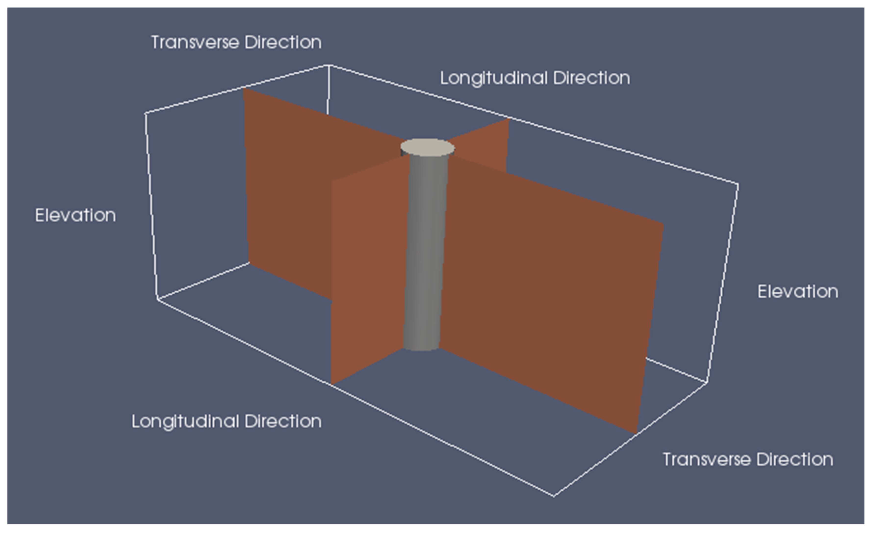
To analyze the velocities and vortexes associated with the flow, two main vertical planes of the channel were designed. The first of these plains corresponds to the longitudinal axis (flow development) passing through the center of the pile from the beginning of the channel to its end. The second is associated with the axis perpendicular to the channel, as shown in Figure 2.

As the first stage of the analysis conducted on the results obtained from the numerical model, the velocity fields along the channel were inspected in order to identify patterns in spatiotemporal flow performance. Subsequently, for each of the planes traced around the cylindrical pile (see Figure 2), the vorticity’s average performance was determined and the associated streamlines were traced to study and analyze the average performance of the horseshoe vortex. Additionally, eight monitoring stations were defined to obtain the vertical distribution of the flow velocity Figure 1 indicates the distribution of these stations, which is concordant with the methodological approach of Miles et al. [51].

Moreover, the amplification of the shear stress (${\alpha }_{\tau }$) around the pile was determined, associated with the average flow conditions and (on a Cartesian plane) based on the numerical domain bed, prior to scour. For such purposes, the proportion of the bed shear stress (${\tau }_0$) and the undisturbed bed shear stress (${\tau }_{\infty }$) according to Equation (25) were considered. To determine ${\tau }_0$ and ${\tau }_{\infty }$, the shear velocity was computed by the numerical model in the bed’s nearest cell for two locations: around the pile $\left(u_{*T,pile}\right)$ for the calculation of ${\tau }_0$ and 2 meters downstream of the inlet ($u_{*T,inlet}$) for ${\tau }_{\infty }$.

The relation employed for the bed shear stress estimations corresponds to the conventional hydraulic definition described in Equation (26) for ${\tau }_0$ and Equation (27) for ${\tau }_{\infty }$, where $u_{*T,inlet}$ or $u_{*T,pile}$ corresponds to the total bed velocity, determined from the longitudinal and transverse velocity vector magnitude.

$${\alpha }_{\tau }=\frac{\left|{\tau }_0\right|}{{\tau }_{\infty }}$$

(25)

$${\tau }_0=\rho u_{*T,pile}^2$$

(26)

$${\tau }_{\infty }=\rho u_{*T,inlet}^2$$

(27)

2.4. Scour around a Cylindrycal Pile

Using a simulated scenario for the study of hydrodynamics, the scour around the pile was estimated by considering a bed composed of spherical sediments with diameter of 0.38 mm ($d$), 2650 Kg/m³ in density, a 30° angle of repose, and a dimensionless critical shear stress (${\tau }_{cr}^{*}$) equal to 0.036, in order to make the results obtained in this investigation for E01 and E02 comparable to those previously presented by Qi and Gao [26].

The scour estimation using the numerical model was activated during the last 25 minutes of the hydrodynamic modelling ($S_1$), to obtain enough information at the beginning of the simulation for the immobile bed condition and, subsequently, the associated condition for the mobile bed.

The features of the numerical tests conducted on the scour around the modeled cylindrical pile are summarized in

Table 6. General characteristics of numerical tests of scour modeling.

Case	${\mathit{\tau }}_{\mathit{c}}^{*}$	${\mathit{\tau }}_{\mathit{w}}^{*}$	${\mathit{\tau }}_{\mathit{w}\mathit{c}}^{*}$	$\frac{{\mathit{\tau }}_{\mathit{w}\mathit{c}}^{*}}{{\mathit{\tau }}_{\mathit{c}\mathit{r}}^{*}}$	Regimen
E01	0.023	0.003	0.023	0.63	Clear water
E02	0.023	0.003	0.023	0.63	Clear water
E03	0.021	0.005	0.021	0.58	Clear water
E04	0.021	0.005	0.021	0.58	Clear water
E05	0.025	0.008	0.025	0.69	Clear water
E06	0.025	0.008	0.025	0.69	Clear water
E07	0.004	0.008	0.004	0.15	Clear water
E08	0.004	0.008	0.004	0.15	Clear water

. The parameters associated with the incipient transport of sediments for the combined regimen of waves and currents have been estimated according to the methodology extensively described in Soulsby [52]. The fundamental equations for estimating shear stress are described below in summary.

Bed shear stress due to the combined action of waves and currents was estimated according to Equation (28), where ${\tau }_c$ is shear stress considering only the action of currents, while ${\tau }_w$ corresponds to the shear stress for waves alone. The shear velocity ($u_{*}$) was determined based on a resistance law according to Equation (31), where $U_B$ is the bulk velocity of the flow due to the current. The wave boundary layer velocity ($U_{fm})$ is defined in Equation (32), where $f_w$ is the friction factor, which was determined according to Fredsøe and Deigaard [53] (page 25).

$${\tau }_{wc}={\tau }_c\left[1+1.2{\left(\frac{{\tau }_w}{{\tau }_c+{\tau }_w}\right)}^{3.2}\right]$$

(28)

$${\tau }_c=\rho u_{*}^2$$

(29)

$${\tau }_w=\frac{1}{2}\rho f_w{U}_{fm}^2$$

(30)

$$\frac{u_{*}}{U_B}=\frac{1}{7}{\left(\frac{d}{h}\right)}^{\raisebox{1ex}{$1$}\!\left/ \!\raisebox{-1ex}{$7$}\right.}$$

(31)

$$U_{fm}=\sqrt{\frac{f_w}{2}}{U}_m.$$

(32)

The shear stress values associated with currents, waves and the combined action of both were nondimensionalized according to Equation (14). The results are presented in Table 6.

Considering that the numerical modeling duration of the scour was 25 minutes and that in this time scale the equilibrium condition was not reached, a projection was made via the equation proposed by Sheppard et al. [54], which corresponds to a four-parameter exponential function for the extrapolation of the equilibrium scour depth ($S_t$), which is presented in Equation (33) where $a_i$ corresponds to the adjustment coefficient $i$ of the equation by Sheppard et al. [54]. This approach was also used by Qi and Gao [20], with experimental data.

$$S_t=a_1\left[1-\exp \left(-a_{2}t\right)\right]+a_3\left[1-\exp \left(-a_{4}t\right)\right].$$

(33)

The equilibrium scour was compared with the results presented by Qi and Gao [26], Sumer and Fredsøe [25], Raaijmakers and Rudolph [15], Sumer et al. [55], and Mostafa and Agamy [56] to check whether the numerical results obtained are concordant with the experimental data developed by other authors.

3. Results

3.1. Hydrodynamics Calibration Test

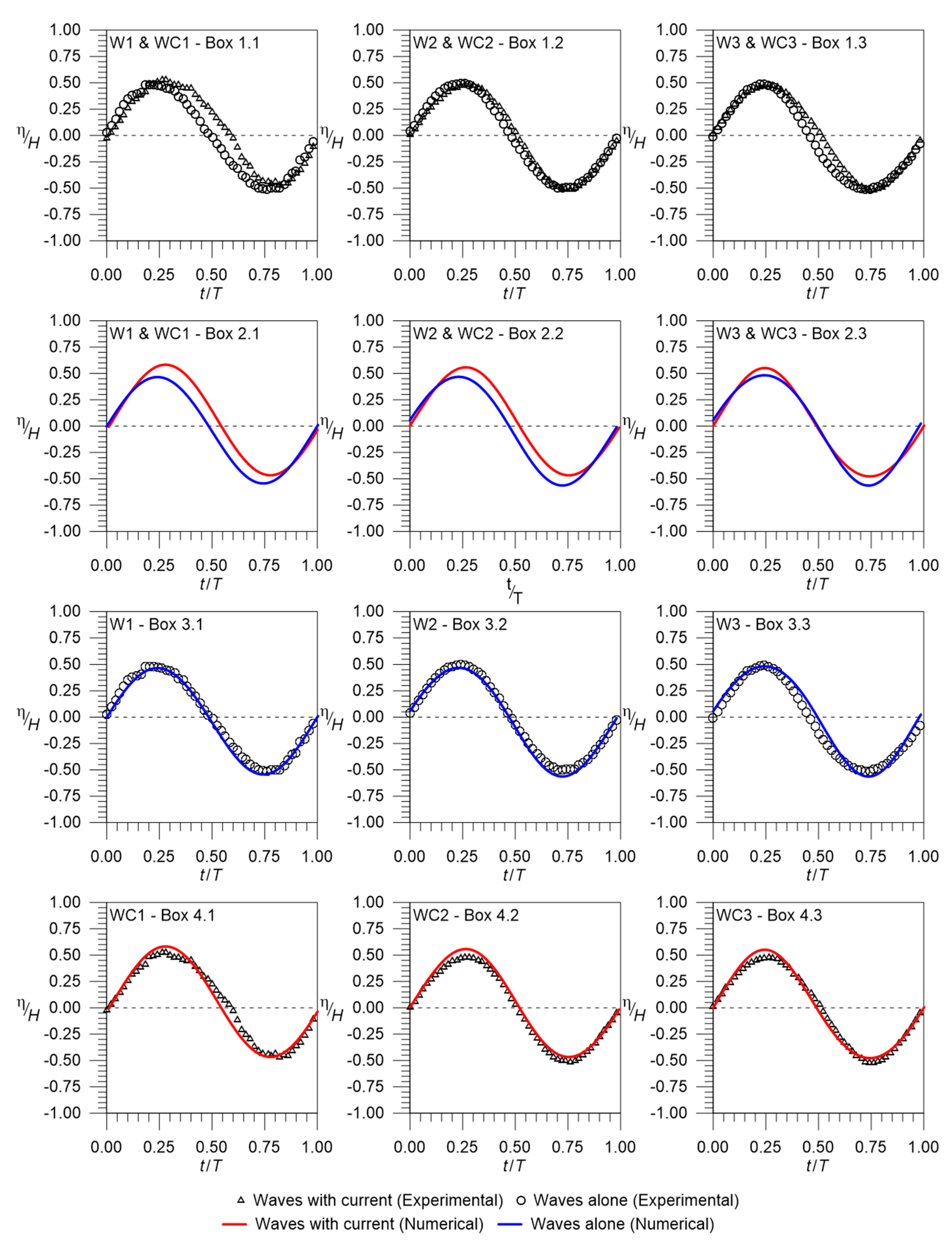
The hydrodynamic calibration process for the numerical model REEF3D is as follows. Figure 3 shows the results obtained by numerical modeling and those reported by Umeyama [3], based on experimental data, for a domain forced by waves and a mixed domain of wave and currents. The comparison variable corresponds to the instant surface elevation ($\eta$) nondimensionalized with the wave height ($H$) as a nondimensional time function ($\raisebox{1ex}{$t$}\!\left/ \!\raisebox{-1ex}{$T$}\right.$), with $T$ as the period. The physical sense of the variable $\raisebox{1ex}{$\eta $}\!\left/ \!\raisebox{-1ex}{$H$}\right.$ corresponds to the fraction of the increase or decrease in the water surface and, evidently, the maximum and minimum fractions are the descriptors of wave asymmetry. The variable $\raisebox{1ex}{$t$}\!\left/ \!\raisebox{-1ex}{$T$}\right.$ corresponds to an indicator of the wave time fraction being simulated.

A comparison between the experimental data for cases where waves are acting alone (W1 to W3, illustrated with circles) and those for waves and currents (WC1 to WC3, illustrated with triangles) are shown in Figure 3, boxes 1.1 to 1.3. Here, it can be deduced that a codirectional current modifies the wavelength and amplitude of the wave. The numerical results are found in Figure 3, boxes 2.1 to 2.3, both for a flow with waves (blue line) and for waves and currents (red line). Thus, it can be verified that the wavelength and amplitude are modified between both flows, as shown in the experimental data (Figure 3, box 1.1 to 1.3). The results of the comparison between the numerical modeling REEF3D and the experimental data provided by Umeyama [3] are included in boxes 3.1 to 3.3 for waves acting alone, while waves and currents acting together are shown in boxes 4.1 to 4.2.

When analyzing numerical and experimental data associated to waves acting alone (W1 to W3), all model cases were able to adequately reproduce the maximum and minimum wave amplitude, as well as its temporal evolution within a wave time coinciding with the necessary time to reach the peak, the zero crossing time and the time to reach the minimum. Taking into account the difference in the estimation of the crest and trough, for the waves and currents (WC1 to WC3), it can be observed that the numerical model slightly underestimates the experimental data, but at a magnitude of less than one millimeter (around 2% error).

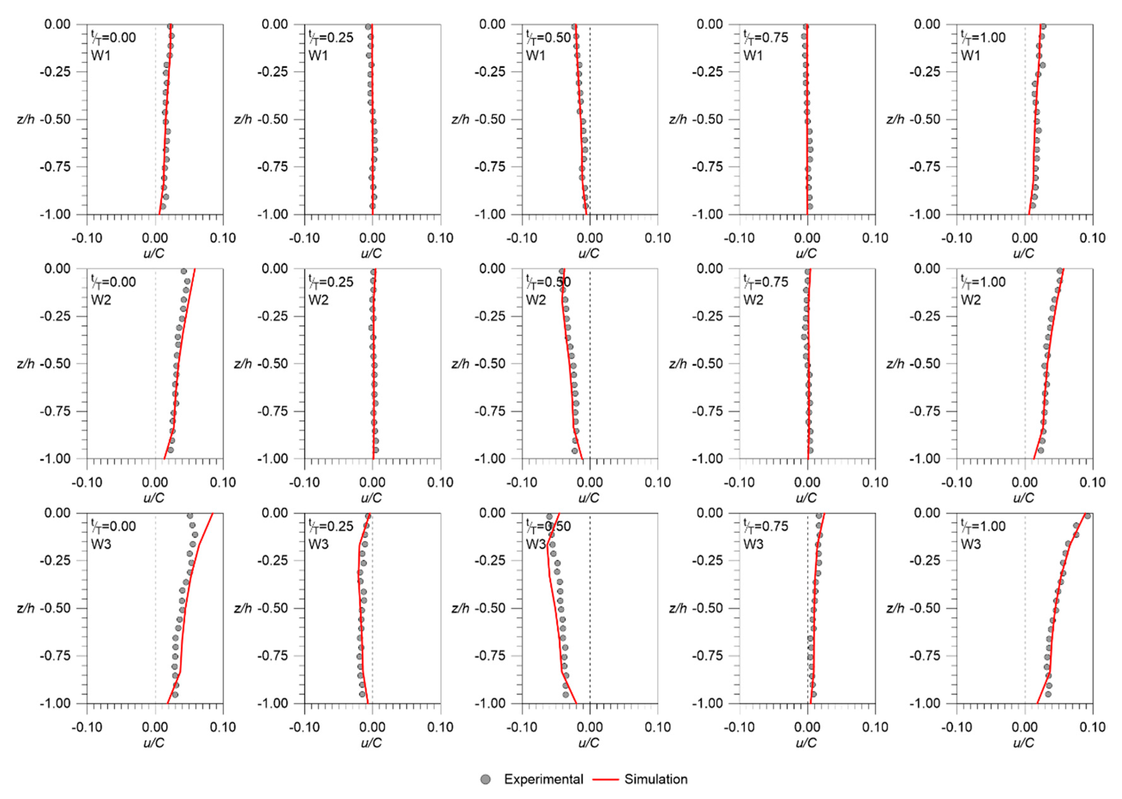
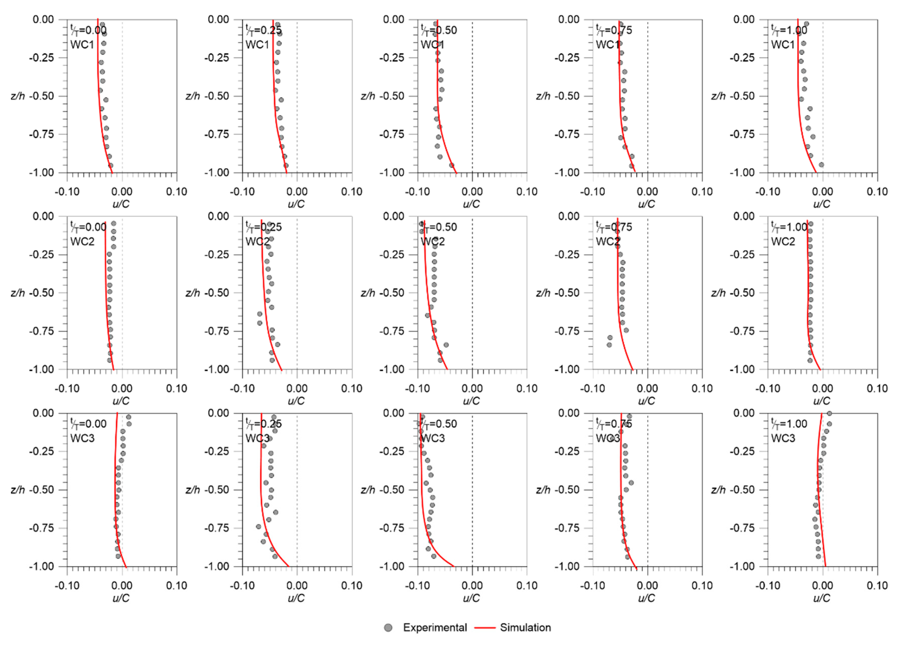
The vertical profiles for the instant velocity associated with each of the simulated cases in the present investigation (which were experimentally registered by Umeyama [3]) are compared in Figure 4 for waves acting alone and in Figure 5 for waves and currents combined. Both figures illustrate four instants of time for each simulated case, ordered from left to right and corresponding to $t/T$ = 0.00, 0.25, 0.50, 0.75, and 1.00.

The results of the comparison of numerical and experimental data considered in the presence of waves alone (Figure 4) reflect a high consistency between vertical and temporal behavior, as the model is capable of adequately representing the flood direction (negative $u/C$) and the ebb direction (positive $u/C$). The experimental and numerical data show equivalent vertical structures for the velocity profile, with a slight increase toward the surface, which is evidenced in a greater proportion when analyzing the case with the highest wave (W3).

Near the bed, the current magnitudes determined based on the numerical model coincide with those determined by experimental means, showing slight differences between the simulated and instrumental data.

The detected differences for $t/T$ = 0.25 and 0.75 show a low magnitude. However, the flood and ebb conditions reached different magnitudes described, as follows. For the W1 case, the maximum difference in the nondimensional velocity ($u/C$) obtained by the ebb direction was 0.004 ($t/T$ = 1.00), while for the flood direction it was −0.001. For the W2 case, the differences fluctuated between −0.005 and −0.011.

Greater differences between the numerical model and experimental data were found for the W3 case for $t/T$ = 0.00, which is produced at the water surface. Meanwhile, near the bed, the greatest difference in $u/C$ was 0.015 for $t/T$ = 1.00.

In Figure 4, the maximum and minimum velocities are not at 0.25 and 0.75 $t/T$ respectively, because the wave phase effect on the initial condition was adjusted to represent the same oscillatory flow that Umeyama [3] reported in his research.

When incorporating a codirectional current to waves, Figure 5 shows that the vertical velocity distribution along the channel only shows the flood direction because the currents control the hydrodynamics. This can be confirmed by calculating the flow relative velocity proposed by Sumer and Fredsøe [26] ($U_{cw}$), which offers results equal to 0.84, 0.70, and 0.60, for WC1, WC2, and WC3, respectively.

In general terms, the numerical model adequately captured the behavior of the velocity profile, showing a greater similarity between the currents near the bed and those obtained toward the free surface. Compared to the hydrodynamic scenarios, where only waves were present, the differences found for the dimensionless velocity ($u/C$) have a greater magnitude when the current is incorporated in the centre, reaching 0.010 for WC1, −0.017 for WC2, and −0.037 for WC3.

The previous results correspond to the scenarios of interactions between waves and currents without the incorporation of a circular pile blocking the flow. However, they allow us to confirm that the numerical model is capable of representing the complex hydrodynamics resulting from the combined action of both components (waves and currents). To strengthen this analysis, the results of the model for a circular pile in the flow are shown next.

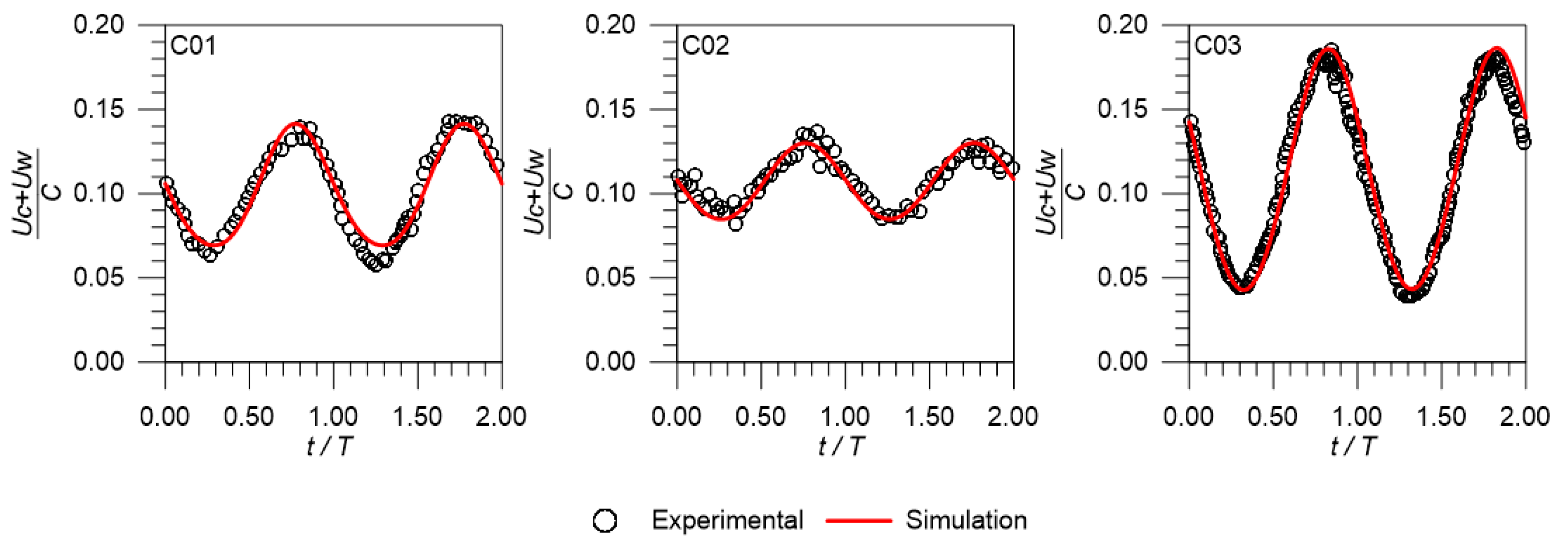
The results of the comparison of the numerical model with the experimental data obtained from Qi and Gao [26] are presented in Figure 6, which considers the total flow velocity ($U_c+U_w$) non-dimensionalized with the characteristic velocity ($C$). Based on this comparison, it was observed that the numerical model was able to represent the dynamic behavior of the combined flow velocity, for the different characteristics of the simulated waves and currents. In test case C01, it can be observed that the numerical model predicted slightly higher velocities in the trough located between 1.00 $<t/T<$1.50, $(U_c+U_w)/C$ (equal to 0.02). This result, however, was not observed in cases C02 and C03. Hence this case does not correspond to the numerical model configuration.

It is important to emphasize that the total flow velocity measurements experimentally obtained by Qi and Gao [26] were registered upstream from the pile at a distance of 20$D$. Ergo, the effects of the opaque structure on the velocities field would not be shown in their behavior. Therefore, this comparison (Figure 6) complements that previously shown in Figure 3 for the instant surface elevation. Thus, the numerical model is capable of representing the wave and current interactions in a freestream.

The effects on the velocity fields caused by the cylindrical pile in a flow field with waves perpendicular to the currents obtained from the numerical model were compared with data provided by Miles et al. [51]. The results for which waves and currents come from perpendicular directions are shown in Figure 7 (associates with case C04). When analyzing monitoring station P1, a high consistency is observed between the velocity profiles modeled (red line) and experimentally obtained data (circles), highlighting that the model is capable of representing the mean velocity near the bed and in the vertical direction as well. Equivalent performance was also verified for P2 and P8, which corresponds to the monitoring stations exposed to the current direction.

In station P4, it is noted that the numerical model may have slight differences in its vertical velocity distributions for elevation range, here $z/h$ is equal to −0.98 to −0.96, which is not clearly presented in the other velocity monitoring stations. This performance detected in station P4 may be caused by the combined wake effect due to currents and waves, since geometrically this location is completely downstream of both forcings (associates with case C04).

3.2. Hydrodynamics Behaviour of the Flow Around a Cylindrycal Pile

The results obtained for the spatio–temporal evolution of the velocity and vorticity fields for case E07 are illustrated in Figure 8. These results consider four instants in time that allow us to visualize the interaction between the flow and the pile. All charted variables have been nondimensionalized by test characteristic scales. For example, the longitudinal and the vertical axes have been made dimensionless with the pile diameter, and, the beginning of the coordinated system has been placed at the center of the pile. The velocities ($u$ and $w$) have been made dimensionless with the characteristic velocity ($C$). Vorticity (${\omega }_x$, ${\omega }_y$, and ${\omega }_z$), on the other hand, was nondimensionalized by the integral temporal scale of the experiment and corresponds to the proportion $D/C$.

In Figure 8, in the first instant of time (Time 1 in Figure 8), it can be observed that the free surface is on a trough nearby the pile where the longitudinal velocity is mainly an ebb type, which usually form a horseshoe vortex when interacting with the incoming boundary layer. Descending velocities are developed in the vertical axis and near the pile, which may be associated with the down-flow.

As time progresses and the crest approaches the pile (Time 2 in Figure 8), the longitudinal velocity starts to diminish its magnitude (nearing zero), thus reflecting the oscillating effect, since this hydrodynamic behavior is an indicator that both ebb and flow can be present based on the phase of the wave. Contrary to the previous instant, the vertical velocity near the pile shows a positive magnitude, which would not produce down-flow and would consequently modify the horseshoe vortex behavior, as follows.

At time instant 3 (time 3 in Figure 8), the wave crest interacts directly with the pile, developing longitudinal velocities mainly oriented downstream the pile, while the vertical component of the velocity is once again oriented toward the bed, thus producing a down-flow. This is maintained for as long as the wave interacts with the pile during the crest phase (time 4 in Figure 8), while the longitudinal velocity changes to an ebb direction.

The association of the main component of the vorticity with the cross vorticity (${\omega }_{y}D/C$) is obtained from the vorticity development near the pile and the adjacent bed for the four illustrated instants of time in Figure 8. Thus, that the minimum intensities occur under the trough, while in the crest there is a general tendency to maximize these intensities. When the crest is approaching the pile, it is observed that in the bed (upstream), a cross vorticity structure with a positive magnitude approaches the pile, and, conversely, the cross vorticity considerably diminishes its magnitude when the trough moves through the pile. The geometrical characteristics of this cross vorticity structure mainly present a greater longitudinal than vertical development.

The vorticity behavior upstream from the pile (described above) corresponds to the horseshoe vortex, and its intermittence would be conditioned by direction changes of the vertical and longitudinal velocity.

The downstream sector under the pile showed a vorticity behavior (${\omega }_{x}D/C$ and ${\omega }_{z}D/C$) with alternate structures (positives and negatives) and a greater development in the vertical axis than in the horizontal axis, compared to the cross vorticity. This spatio–temporal development could be associated with vortex shedding, resulting from structure-fluid interactions.

Based on a general analysis of the information obtained from the numerical modeling (a visual inspection of the results), there are no significant differences in the mean spatio–temporal behavior of the streamlines, vorticities, and velocity field; hence, these element can be broadly described by the specification of one of the eight case simulations, with scenario E01 selected for this effect.

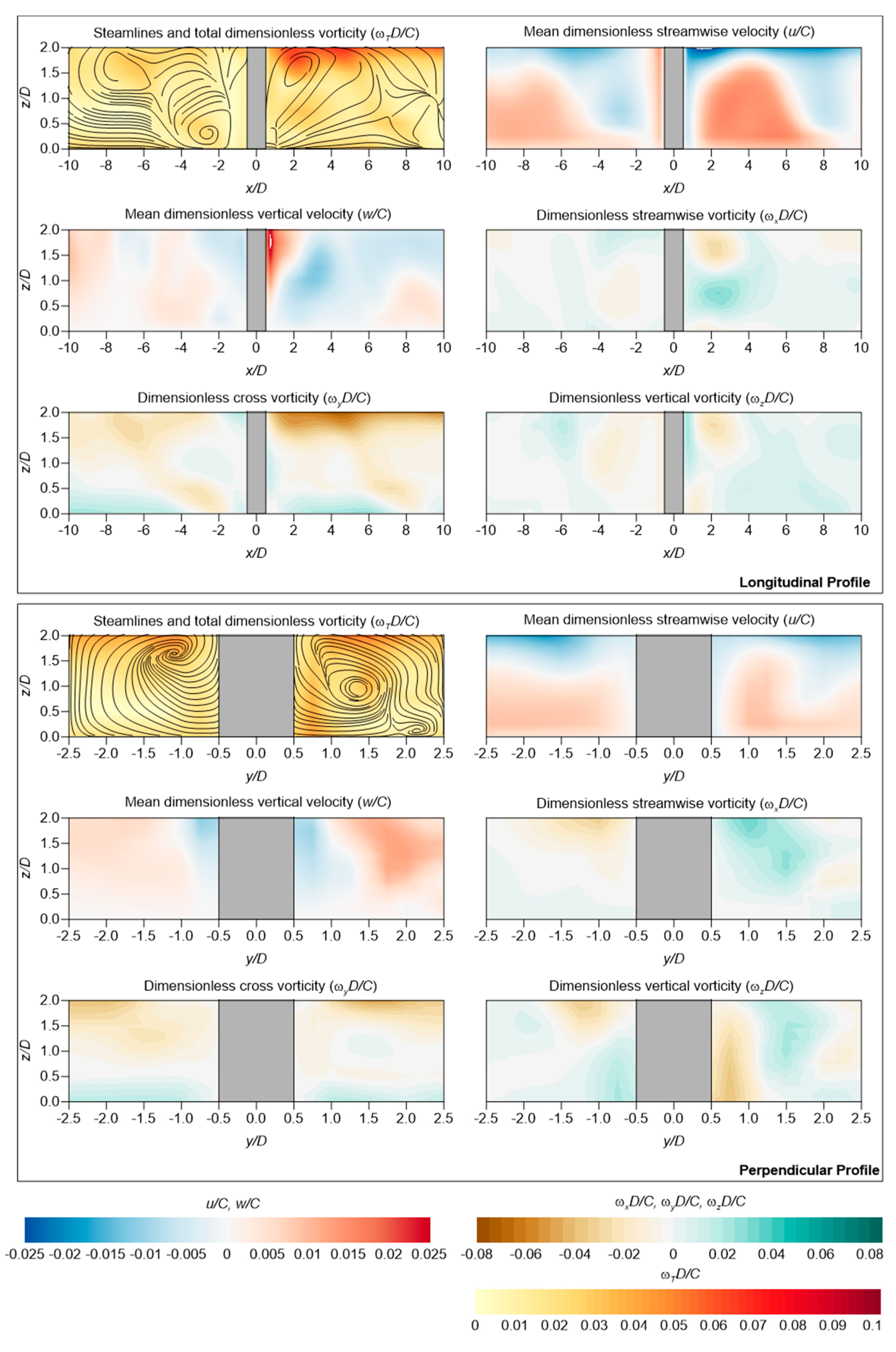
The characteristic results of scenario E01 are presented in Figure 9. Unlike Figure 8, which illustrates the behavior from the free surface to the bed, in this section, the analysis focused on the bottom to obtain the characteristics of the hydrodynamics that might be responsible for sediments transport and, consequently the scour around the pile.

Figure 9 is divided into two main boxes. The upper box illustrates the flow characteristics in the longitudinal profile of the channel, while the lower box illustrates the transverse section. Both have included the streamlines and total vorticity (vector addition, ${\omega }_{T}D/C$), the mean velocity along the channel ($u/C$), the vertical mean velocity ($w/C$), the mean vorticity along the channel (${\omega }_{x}D/C$), the transversal mean vorticity (${\omega }_{y}D/C$), and the vertical mean vorticity (${\omega }_{z}D/C$) in a nondimensionalized manner.

The total vorticity in the longitudinal profile and flow lines reflect the presence of a horseshow vortex as the main structure upstream the pile ($x/D$ < 0), this structure approximately centered at $x/D$ = −2.6 and $z/D$ = 0.3. This vorticity system also reflects the average behavior of the flow longitudinal velocity, as in the zone equivalent to the horseshoe vortex location, $u/C$ has negative values that are driven by the vortex counter clockwise rotation. Additionally, $w/C$ also reflects the horseshoe vortex effects, since negative magnitudes of the vertical velocity (known as the down-flow) can be revealed near the pile. Meanwhile, at a distance lower than $x/D$ = −2.6, the down-flow becomes positive (mainly driven by the counter clock turn of the vortex).

The pile downstream area ($x/D$ > 0) in the mean streamline condition showed a rotational centered structure at around $x/D$ = 2.4 and $z/D$ = 1.6, which is related to the vortex shedding and could produce alterations in the mean field of the vertical and longitudinal velocities. Longitudinally, near the pile, a flow could be produced toward it, mainly caused by the momentum balance that would be developed at an approximate distance of $x/D$ = 1.2. Then, a positive direction of the flow velocity up to a distance of $x/D$ = 6 would be present, to subsequently re-adopt a negative velocity; since this behavior is associated with vortex shedding, as stated previously.

Vertical velocities in the downstream area show that, nearby the pile, the flow moves upwards. Meanwhile, an $x/D$ = 2.7 distance would make the vertical velocity negative. This and the flow line behavior could be caused by clockwise rotation and related to the formation of vortex shedding.

Analyzing the transverse section of the flow in Figure 9, clear that in the mean streamlines, a horseshoe vortex system develops around the pile, with a longitudinal component of mainly positive velocities near the pile. In the case of a vertical component, these velocities would be negative. This means that: a downstream flow component is present once the horseshoe vortex surrounds the pile, and it remains near the bed pushed by the flow vertical velocities.

The presence of structures concordant with the horseshoe vortex around the pile is shown by the transverse vorticity (${\omega }_{y}D/C$). Thus, the vertical development of these structures is limited to an approximately height of $z/D$ = 0.5 from the bed. The mean vorticity fields obtained for vertical and longitudinal components are congruent with the classical description of the flow around the cylindrical piles for a permanent flow, which has been widely addressed in the literature [1,2,3,4].

The mean velocity vertical profiles for monitoring stations P1 to P8 are presented in Figure 10 for each modeled scenario. From this, it can be observed that the mean characteristics of the codirectional currents and wave velocity profiles are not significantly different under opposite flow conditions in either of the proposed scenarios (those controlled by currents or those controlled by waves).

Clear evidence of this phenomenon is shown in P5 (Figure 10), which corresponds to a downward station for codirectional currents and waves and an upstream station for waves in opposite flow scenarios. In each case, the station presented the smallest flow magnitudes, indicating that for all the simulated scenarios of station P5, currents dominate the flow, according to the flow relative velocity ($U_{CW}$) proposed by Sumer and Fredsøe [25], this result indicates that a combined regimen is present. This aspect will be further addressed in the analysis of the results.

It is important to note that the currents are symmetrical based on the pile geometrical characteristics (cylinder) and the studied flow. Figure 10, shows that the velocity profiles of station pairs P2 with P8; P3 and P7; and P4 and P6 are concordant not only in their magnitudes but also in their vertical axis. Thus, describing only one of the stations associated in a pair is sufficient to understand the flow around the pile.

The velocity profiles for both codirectional and opposite cases reached their maximum value in station P3 (P7), mainly due to the contraction of flow lines producing accelerations, thereby increasing the velocities from station P1 towards P3 (P7), followed by a gradual decrease from station P3 (P7) towards P5.

In light of the results described above, and for the simulated scenarios, the hydrodynamics around a pile for combined flow of waves and currents (codirectional and opposite) should behave like a normal flow around a cylinder due to its steady state flow, which is widely described in the literature.

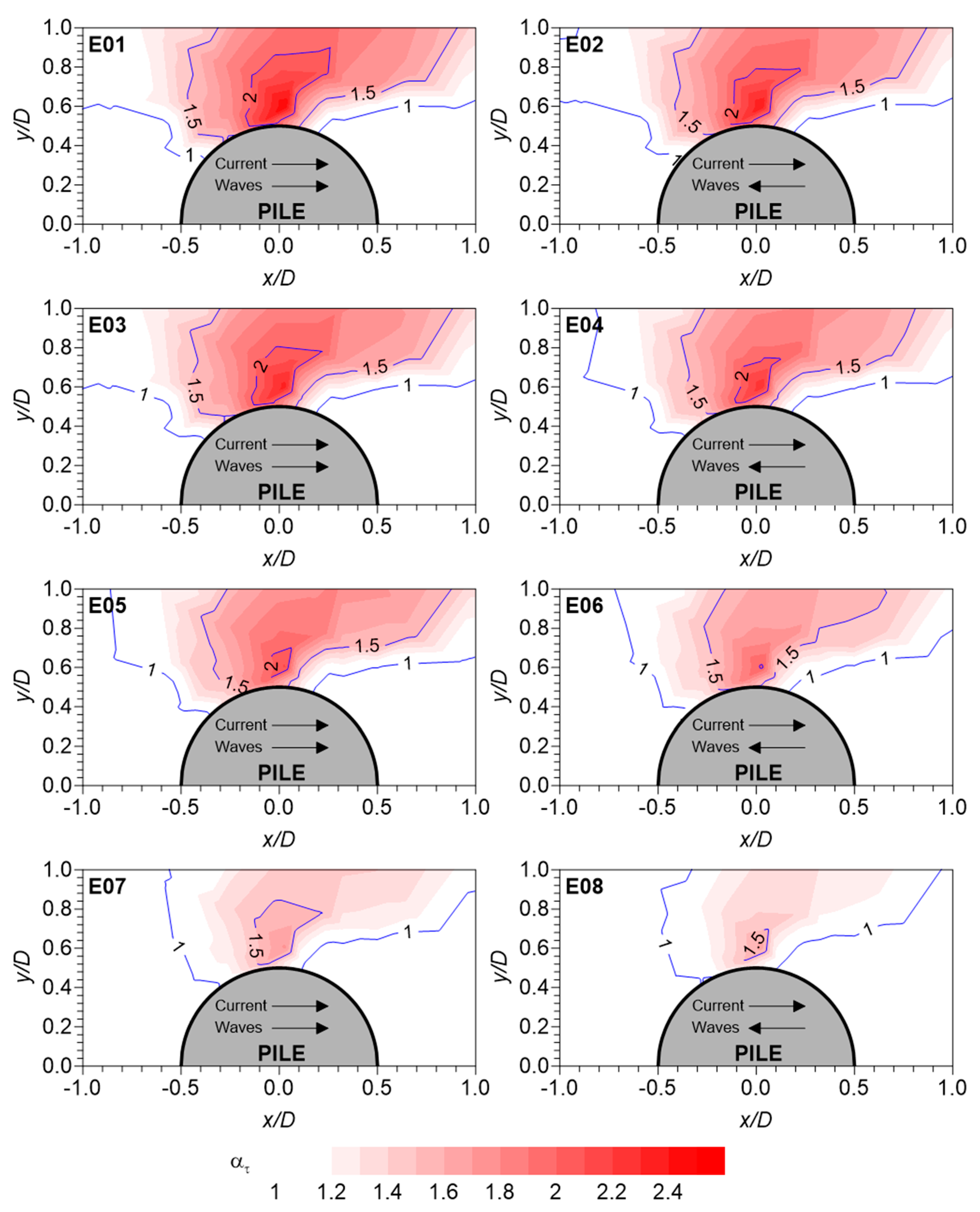
The amplification of the mean shear stresses (${\alpha }_{\tau }$) made dimensionless with an undisturbed bed shear stress around a cylindrical pile is shown in Figure 11 for each of the simulated cases, in which the left column shows codirectional currents and waves cases and the right column shows the opposite current and wave cases.

The maximum amplifications of the main bed shear stress were produced in the pile lateral edge and reached magnitudes of 2.5 for codirectional and opposite currents and waves cases. Nevertheless, when waves act on the current in an opposite direction, the amplification zone coverage is reduced (smaller area) compared to the codirectional current and wave cases. As a general trend, the amplification obtained shows that shear stress gradually decreases from hydrodynamic scenarios dominated by currents (E01 and E02) to those dominated by waves (E07 and E08).

Analyzing the results of E01 and E02, the differences found between the spatial distributions of the bed shear stress are not significant when the waves act codirectionally with currents or when they are opposite. No significant movements were noticed in the maximum amplification localization. This means no direct influence of the waves flow or ebb was found for the development of the shear stress in the bottom.

A behavior equivalent to that described for E01 and E02 was identified in E03, E04, E05, and E06, that is, no influence of the waves in the mean bed shear stress distribution was evidenced, even though according to $U_{cw}$ waves domain. In general hydrodynamics, should become more significant when transiting from scenario E01 to E07 and E08. In these last scenarios (E07 and E08), the lowest amplifications of the mean bed shear stress were obtained, which were 1.5.

3.3. Scour around a Cylindrycal Pile

This section presents the analysis results of the scour around the pile. Figure 12 presents the dimensionless scour time series ($S/D$) obtained experimentally by Qi and Gao [26] and the series resulting from the numerical model, for codirectional (E01) and opposite (E04) waves and currents.

The information for the codirectional flow (E01) illustrated in Figure 12 shows a strong agreement between the experimental and simulated data, in its temporal evolution (curve form) and in the magnitude reached by the dimensionless scour. For example, after 10 minutes of simulation the model reached a magnitude of $S/D$ = 0.173, and the experimental data reached a magnitude of $S/D$ = 0.169 (2.4% of the relative error).

The comparison of numerical data versus experimental data for the dimensionless scour with and opposite flow (E04) illustrated in Figure 12 (as the previously described for E01) showed a strong correspondence in both its the temporal evolution and the magnitude reached. For example, within 20 minutes, the experimental data shows the dimensionless scour would be 0.146, while the numerical model showed that the scour would be 0.139 (4.8% of the relative error).

The generality of the results obtained and presented in Figure 12 indicates that the scour would be greater when the flow acts codirectional to the waves and currents than in the opposite case. The latter is supported by the results summarized in

Table 7. Adjustment parameter for equilibrium scour estimate and the results obtained from the numerical simulation.

Case	${\mathit{a}}_1$	${\mathit{a}}_2$	${\mathit{a}}_3$	${\mathit{a}}_4$	$\frac{{\mathit{S}}_1}{\mathit{D}}$	$\frac{{\mathit{S}}_{\mathit{t}}}{\mathit{D}}$	$\frac{{\mathit{S}}_{\mathit{t}}}{{\mathit{S}}_1}$
E01	0.095	0.408	0.423	0.029	0.251	0.518	2.064
E02	0.330	0.078	0.006	1.078	0.161	0.336	2.083
E03	0.330	0.091	0.100	0.091	0.304	0.430	1.414
E04	7.663	0.230	−7.365	0.234	0.151	0.298	1.976
E05	2.553	0.068	−1.878	0.070	0.132	0.675	5.120
E06	0.755	0.002	0.149	0.089	0.110	0.626	5.711
E07	0.020	0.058	0.083	0.070	0.085	0.103	1.213
E08	0.081	0.067	−0.006	0.416	0.060	0.075	1.242

column$S_1/D$, which is the dimensionless scour obtained in the last time step of the numerical model. Additionally, Table 7 lists results for the adjustment coefficients of the equilibrium scour equation from Sheppard et al. [54] ($a_1$ to $a_4$), the equilibrium dimensionless scour ($S_t/D$), and the relative scour factor ($S_t/S_1$). A similar method was used by Qi and Gao [26] but with experimental data.

The relative scour factors indicated in Table 7 were greater in cases where the flow velocity defined at a distance of $z=D/2$ ($U_c$) was greater. This mean that the scour obtained from the numerical model of a 25 minutes sediment transport and resulting morphodynamics evolution of the bed, is very different from the equilibrium in cases whit greater flow magnitude.

The latter may be associated with major currents acting on the center, producing major scours and subsequently requiring greater action times in order to reach scour equilibrium [5]. Nonetheless, when magnitudes of the dimensionless equilibrium scour estimated by the equation developed by Sheppard et al. [54] and based on the data obtained here for the 25 minutes simulation are compared with the experimental data obtained by third parties, equivalent results and estimates within an acceptable range of experimental variability are obtained, as shown in Figure 13.

Figure 13 presents a comparison between the numerical data obtained in this article (blue circles for codirectional scenarios and red circles for opposite flows), and experimental ones found in the literature [21,25,26,55,56]. This graph was formed similarly to that presented by Sumer and Fredsøe [25], i.e., the dimensionless equilibrium scour as a function of the Keulegan–Carpenter ($KC$) number for different relative velocity ranges between waves and currents ($U_{CW}$).

From the general analysis of Figure 13, it is observed that, for the range 0.10 < $U_{CW}$ < 0.40, the data obtained from the numerical model implemented in this article would be close to the data obtained by Raaijmakers and Rudolph [21] and Sumer et al. [55] for similar Keulegan–Carpenter numbers (around five) for both the codirectional flow condition and the opposite. This situation repeats in the comparison between ranges 0.40 < $U_{CW}$ < 0.50 and 0.50 < $U_{CW}$ < 0.80, meaning that the data obtained from the results projection of the numerical model toward the equilibrium scour based on the equation of Sheppard et al. [54] allows us to gather magnitudes that can be compared with the experimental records obtained by other researchers, for similar hydrodynamic characteristics.

4. Discussion

The experimental data with no scour provided by Umeyama [3] have been used to compare the numerical results of other authors, such as Zang et al. [30] and Ahmad et al. [31] who used the RANS approach to solve the hydrodynamics of waves and currents acting codirectionally over a grid featuring finite differences with a regular element ($\Delta x$ = $\Delta y$ = $\Delta z)$, which correspond to the methodology applied in this investigation.

For the construction of the numerical domain, Zang et al. [30] utilized $\Delta x$ = 0.002 m to solve the vertical domain in 150 layers, while the configuration applied by the authors of this study considered $\Delta x$ = 0.01 m which determines the 30 layers in the vertical direction for the water flow adopted by Umeyama [3]. Despite of the coarser grid used in this research, the results are consistent with the experimental data for the vertical profile of velocities as well as for the instantaneous surface elevation of the water.

In order to model the scour around cylindrical piles, this study used the same element dimension as Ahmad et al. [31], who proved that the use of an element of 0.01 m is sufficient to estimate the scour under a pipeline [31]. This conclusion was reached by a grid analysis and time convergence study which analyzed the numerical behavior of REEF3D for element sizes of $\Delta x$ = 0.04, 0.03, 0.02, 0.01 and 0.005 m.

The results obtained from the eight simulations (scenarios E01 to E08), showed a low variability of the mean velocity profile around the pile (stations P1 to P8), as illustrated in Figure 10, although these simulations were constructed to represent both, mixed and current or waves dominated environments, according to the criteria of Sumer and Fredsøe [26]. The results associated with the expected bed shear stresses for each of the eight scenarios (see Table 6), show that the effect of the waves on the first six scenarios (E01 to E06) is not significant in the bed dynamics, since the dimensionless shear stress due to waves (${\tau }_w^{*}$) is an order of magnitude less than the dimensionless shear stress due to currents (${\tau }_c^{*}$).

Based on the above, if it is considered that the shear stress is the hydraulic boundary condition to build at vertical profile of flow velocities, and the effect of the current dominates over the waves, it is expected that the first six scenarios present a high similarity for both a co-directional and opposed flow. On the other hand, in the remaining scenarios (E07 and E08), where the dimensionless shear stresses associated to waves and currents are of the same order of magnitude, greater effects on the velocity profile around the pile could be noticed (Figure 10), which would indicate that both the co-directional and opposed flow develop differences in the velocity mean behavior.

This difference between the shear stresses and the Sumer and Fredsøe criteria [26] seems to imply that the use of the dimensionless number called the relative velocity of the current $(U_{CW}$), does not fully describe the domain of the forcing over the total hydrodynamics, a discussion that is presented in the following paragraphs of this investigation.

From the results obtained, it is possible to verify that the presence of waves in the hydrodynamic behavior for scenarios E01 to E06 was less significant than for scenarios E07 and E08. This can be clearly seen in the mean profile analysis, since when the current dominated, the direction resulting from the flow agreed with the streamwise direction, these results were previously described by Feraci et al. [4], who, while performing wave and current test acting orthogonally and without the presence of a pile, obtained results comparable to those obtained in this investigation.

The vertical distribution of the mean velocity illustrated in Figure 10 is consistent with that described by Lim and Madsen [5], who mentioned that although the flow field can be mixed (waves and currents acting together and orthogonally), the velocity distribution can be simply modeled by a uniform return current. The foregoing analysis is also consistent with the results presented by Feraci et al. [6].

The equation by Sheppard et al. [54] was applied to estimate the equilibrium scour based on an extrapolation of the numerical model. These results were similar to those obtained experimentally by other authors, which indicates that the methodology applied as well as the configuration adopted by the numerical model are appropriate to describe the phenomenon under study, not only from the perspective of element size but also for the sediment transport equations applied.

An important aspect to highlight is that this investigation has used the relaxation factor previously applied by Quezada et al. [27], which also allowed the authors to correctly represent the scour for unsteady current and oscillatory flow. According to the results obtained in the current study, this value will also allow us to estimate the scour for uniform and oscillatory flow, not only codirectionally but also opposite. The relaxation coefficient permits in an auxiliary manner effects inherent to the structure of the fluid interaction produced around the pile, thereby improving the estimations of sediment transport and the resulting scour.

Sumer and Fredsøe [26] propose the relative velocity of the current$(U_{CW}$) as a dimensionless number relevant for the description of the scour due to codirectional or perpendicular waves and currents. This is defined in Equation (1), where the current magnitude ($U_C$) is estimated at a height of $D$/2 from the bed, while the velocity of the wave is considered as the maximum value of the undisturbed orbital velocity at the bottom, just above the wave boundary layer ($U_m$). By this dimensionless definition, Sumer and Fredsøe [26] established that values of $U_{CW}$ higher than 0.7 indicate that the current dominates in the center, while waves have a significant effect when$U_{CW}$ is close to zero (cases waves alone) and less than 0.4.

This dimensionless number considers that $U_C$ and $U_m$ are added, independently of the direction of incidence of the currents and waves. In this respect, Sumer and Fredsøe [26] consider a single value of $U_{CW}$ for codirectional and perpendicular flow, if $U_C$ and $U_m$ are the same in magnitude but different in direction.

The above, according the authors of this paper, would not be appropriate as a general indicator of wave and current interaction, nor would their effects on the scour for cases in which the forcings are not codirectional, since when both flows face in the opposite direction, the wave would propagate with greater difficulty and modify the net velocity of the channel, such that the current present in the center would correspond to the residual value of both forcings.

Soulsby [52] and Van Rijn [57] indicates that current wave interactions must be treated in terms of the net current produced between the two forcing agents, which corresponds to an algebraic sum that is usually treated according to Equation (34), where $\varpi$ is the angular frequency, $U_B$ is the bulk velocity of the flow due to the current, $K$ is the wave number, ${\vartheta }^{\prime }$ is the angle between current and wave direction (${\vartheta }^{\prime }$ = 0 for codirectional, and ${\vartheta }^{\prime }$ = 180° for opposing), $g$ is the gravity and $h$ is the water depth:

$$\varpi -U_{B}K\cos \left({\vartheta }^{\prime }\right)=\sqrt{gK\tan h\left(Kh\right)}.$$

(34)

The left term of Equation (34) correspond to the net velocity (defined according the relative velocity between the current and waves). Meanwhile, the right term corresponds to the dispersion relationship of the waves.

From Equation (34) it can be seen that in cases of co-directional or opposite waves, the $cos\left(\vartheta \prime \right)$ changes its sign and therefore, the system net velocity is the sum or subtraction of both forcings. Therefore, defining a dimensionless number that summarizes the wave and current interaction, must include a differentiation when the action is codirectional or when it is counter current.

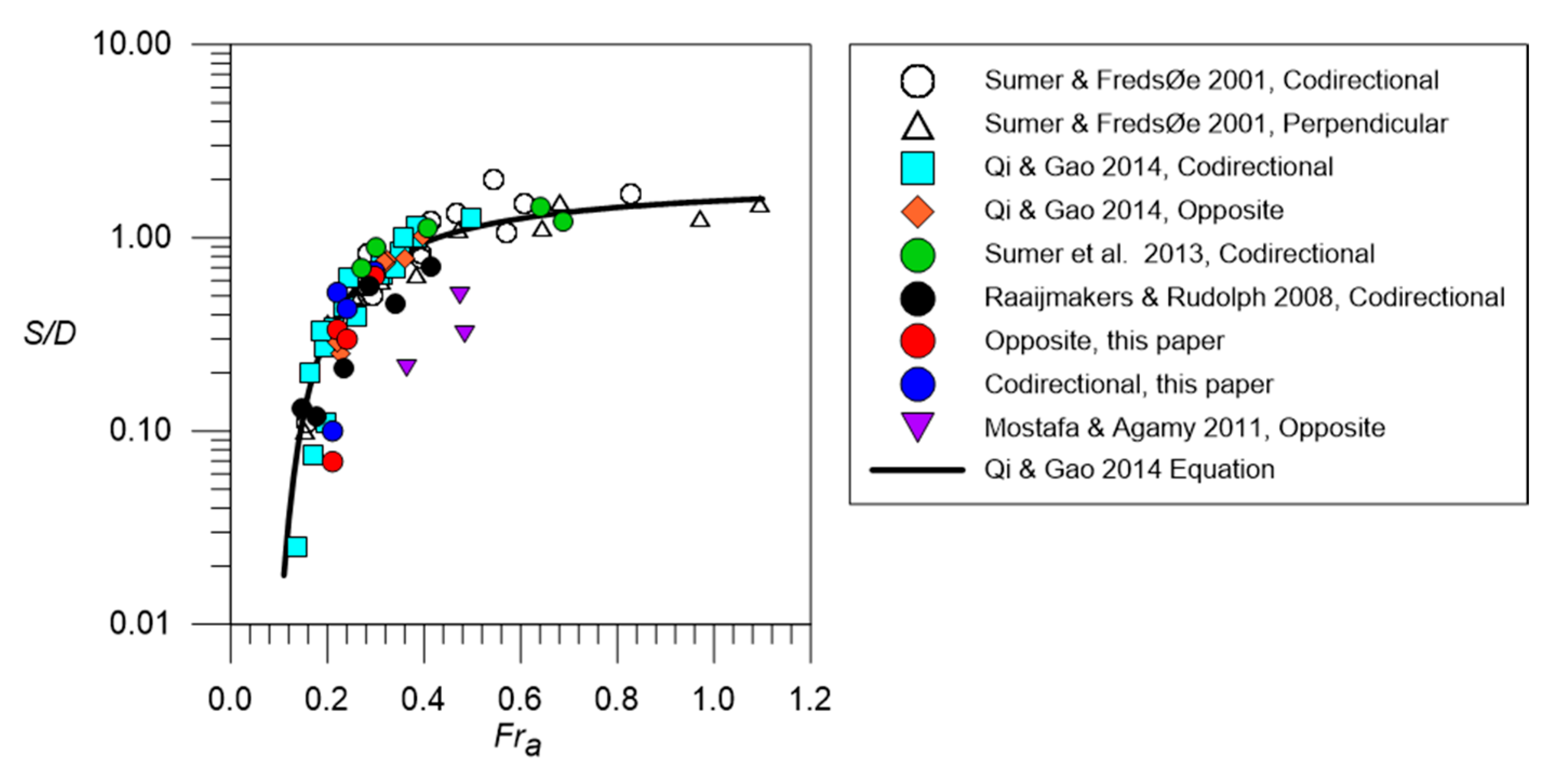
An approximation to the description of scour due to opposite and codirectional currents and waves was conducted by Qi and Gao [58] who, using experimental data, obtained by the same authors in previous works (Qi and Gao [26]) and by third parties as well (Sumer and Fredsøe [18] and Sumer et al. [55]), propose the use of the Froude number ($F_{ra}$) defined in Equation (35), as a function of absolute velocity ($U_a$, defined by Equation (36)) and the pile diameter.

$$F_{ra}=\frac{U_a}{\sqrt{gD}}$$

(35)

$$U_a=U_C+\frac{2}{\pi }{U}_m.$$

(36)

From this analysis Qi and Gao [52] proposed a formula fitted to the experimental data for a dimensionless scour ($S/D$) which is presented in Equation (37) and is valid for the range 0.1 < $F_{ra}$ < 1.1 and 0.4 < $KC$ < 2.6.

$$log\left(\frac{S}{D}\right)=-0.8\exp \left(\frac{0.14}{F_{ra}}\right)+1.11.$$

(37)

A comparison of the numerical results gathered in this paper, the experimental data and the equation proposed by Qi and Gao [58] are shown in Figure 14.

In Figure 14, it is observed that the information available in the literature (experimental) and that generated in this study (numerical) are adequately concordant with the equation proposed by Qi and Gao [58], and such a description may be enough to collect information on the equilibrium scour around a dimensionless number that represents its behavior.

Notwithstanding the above, Qi and Gao [58], as well as Sumer and Fredsøe [26], consider current and wave actions added equally if they act in a codirectional or opposite manner, which, in general, is not consistent with a residual flow estimation that would be generated by the interaction. The foregoing disagrees with the results by Soulsby [52] and Van Rijn [57], who indicate that the sum of the forcing agents must be algebraic, respecting the angle between current and wave direction. Although the arguments are contradictory, both proposals (Qi and Gao [58], Sumer and Fredsøe [26]) compile reasonably well the scour information regardless of the direction. This should be analyzed in greater detail as proposed below.

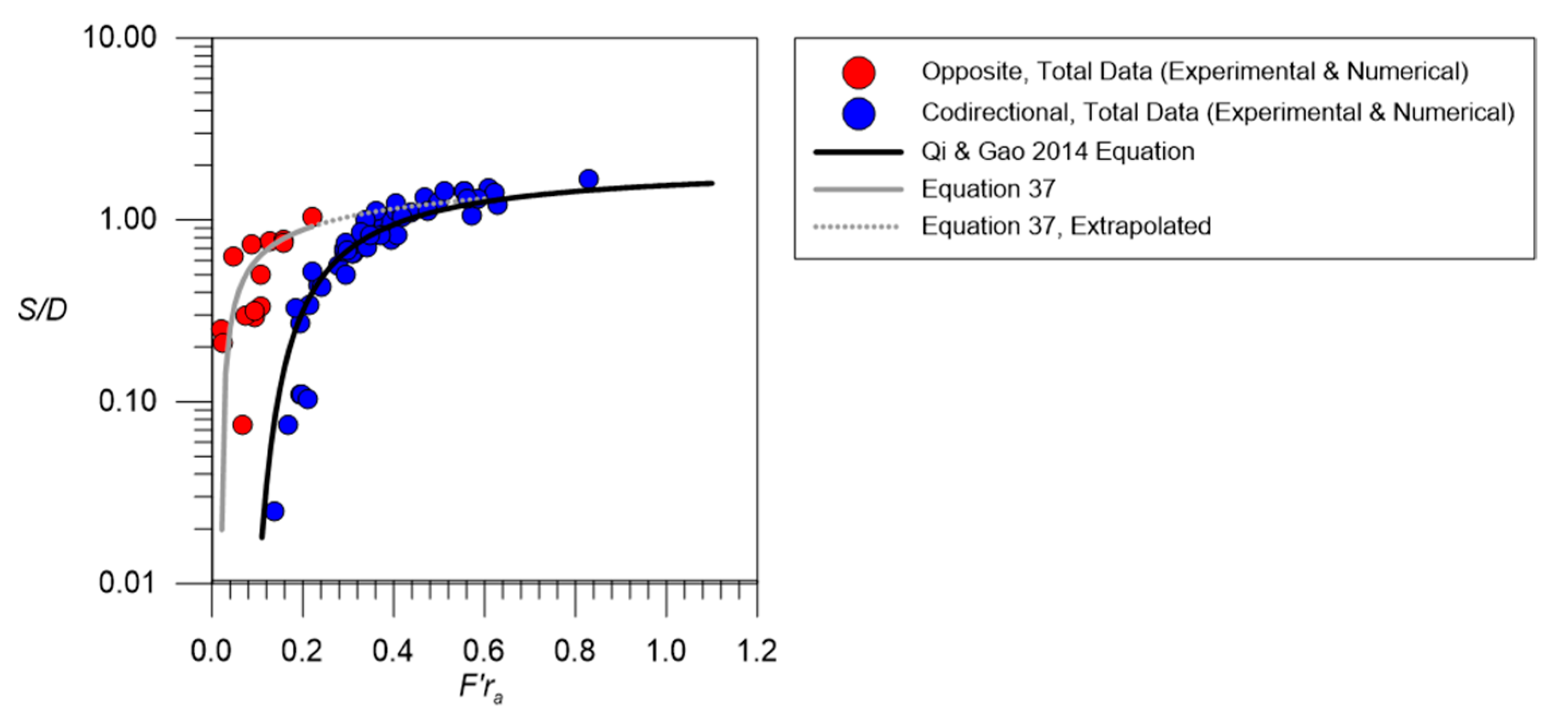
Thus, the Froude number may be rewritten according to Equation (39) if the absolute velocity defined by Qi and Gao [58] is considered, albeit modified according to Equation (38), which is a proposal of the authors of this paper, and where $C_{\phi }$ is a coefficient to describe the flow direction, and where $C_{\phi }$ = 1 describes codirectional flows and $C_{\phi }$ = −1 describe opposite flows.

$$U_a^{\prime }=U_C+\frac{2}{\pi }{U}_m{C}_{\phi }$$

(38)

$$F_{ra}^{\prime }=\frac{U_a^{\prime }}{\sqrt{gD}}.$$

(39)

$C_{\phi }$ was included in order to incorporate the recommendations of Soulsby [52] and Van Rijn [57], in order to consider the effects of waves and currents directionality acting together on the pile.

Considering this proposal and collecting scour data (experimental and numerical from this paper), Figure 15 is obtained. The blue circles indicate codirectional cases and red circles indicate opposite flow cases. Two trends are found in two areas of the figure. The first trend corresponds to codirectional data, which are still represented by the equation proposed by Qi and Gao [58]. Nevertheless, the opposite flow cases are to the left of the codirectional data and apparently adjust to an equation different than that proposed by Qi and Gao [58], which, according to the available data set (experimental and numerical data from this paper) correspond to Equation (39).

$$\frac{S}{D}=0.39LN\left(F_{ra}^{\prime }\right)+1.51.$$

(40)

Equation (40) seems to agree with the solution proposed by Qi and Gao [58] for high values of the Froude number. However, such behavior may be verified by adding new experimental and/or numerical antecedents, which enable us to complement equilibrium scour data in a combined domain of currents and waves acting in opposite directions.

5. Conclusions

A comparison of the results obtained numerically in this research with experimental data from other authors, show that CFD REEF3D adequately models a hydrodynamic field in a combined domain of waves and currents, correctly depicting both the instantaneous water surface and velocities developed by the flow of a freestream and also the flow in the presence of a pile.

The average hydrodynamics determined for each of the simulated scenarios showed that in 6 (E01 to E06) out of 8 cases, currents were the main flow mechanism over the waves, despite the relative velocity of current ($U_{cw}$) proposed by Sumer and Fredsøe [26], which indicate a combined flow regime. This was clearly reflected in the velocity profiles traced in points P1 to P8, where it could be verified that codirectional and opposite flow cases converge to the same vertical distributions of velocity.

The equilibrium scour estimated by the projection of the numerical data with the equation by Sheppard et al. [54], enabled us to estimate values close to those described in the literature and to use the numerical model effectively to solve a time scale lower than the equilibrium. From this projection, it was verified that the dimensionless scour would be less when waves and currents come from opposite directions.

The $U_{cw}$ parameter is an indicator that adequately measures the interactions between of currents and waves under the condition of codirectional flow. However, it is recommended to modify this parameter for currents and waves from opposite directions, since it does not properly account for the interaction of both forcings. For such purposes, it is recommended to use the modified Froude number ($F_{ra}^{\prime }$) proposed in this paper.

References

- Umeyama, M. Reynolds stresses and velocity distributions in a wave-current coexisting environment. J. Waterw. Port Coast. Ocean Eng. 2005, 131, 203–212. [Google Scholar] [CrossRef]
- Umeyama, M. Changes in turbulent flow structure under combined wave-current motions. J. Waterw. Port Coast. Ocean Eng. 2009, 135, 213–227. [Google Scholar] [CrossRef]
- Umeyama, M. Coupled PIV and PTV measurements of particle velocities and trajectories for surface waves following a steady current. J. Waterw. Port Coast. Ocean Eng. 2010, 137, 85–94. [Google Scholar] [CrossRef]
- Faraci, C.; Foti, E.; Marini, A.; Scandura, P. Waves plus currents crossing at a right angle: Sandpit case. J. Waterw. Port Coast. Ocean Eng. 2011, 138, 339–361. [Google Scholar] [CrossRef]
- Lim, K.Y.; Madsen, O.S. An experimental study on near-orthogonal wave–current interaction over smooth and uniform fixed roughness beds. Coast. Eng. 2016, 116, 258–274. [Google Scholar] [CrossRef]
- Faraci, C.; Scandura, P.; Musumeci, R.E.; Foti, E. Waves plus currents crossing at a right angle: Near-bed velocity statistics. J. Hydraul. Res. 2018, 56, 464–481. [Google Scholar] [CrossRef]
- Hjorth, P. Studies on the Nature of Local Scour; Lund University: Lund, Sweden, 1975. [Google Scholar]
- Melville, B.W. Local Scour at Bridge Sites. Ph.D. Thesis, University of Auckland, Auckland, New Zealand, 1975. [Google Scholar]
- Ettema, R. Scour at Bridge Piers. Ph.D. Thesis, University of Auckland, Auckland, New Zealand, 1980. [Google Scholar]
- Chiew, Y.M.; Melville, B.W. Local scour around bridge piers. J. Hydraul. Res. 1987, 25, 15–26. [Google Scholar] [CrossRef]
- Melville, B.W.; Chiew, Y.-M. Time scale for local scour at bridge piers. J. Hydraul. Eng. 1999, 125, 59–65. [Google Scholar] [CrossRef]
- Oliveto, G.; Hager, W.H. Temporal evolution of clear-water pier and abutment scour. J. Hydraul. Eng. 2002, 128, 811–820. [Google Scholar] [CrossRef]
- Link, O.; Pfleger, F.; Zanke, U. Characteristics of developing scour-holes at a sand-embedded cylinder. Int. J. Sediment Res. 2008, 23, 258–266. [Google Scholar] [CrossRef]
- Diab, R.; Link, O.; Zanke, U. Geometry of developing and equilibrium scour holes at bridge piers in gravel. Can. J. Civil Eng. 2010, 37, 544–552. [Google Scholar] [CrossRef]
- Link, O.; Henríquez, S.; Ettmer, B. Physical scale modelling of scour around bridge piers. J. Hydraul. Res. 2019, 57, 227–237. [Google Scholar] [CrossRef]
- Sumer, B.M.; Fredsøe, J.; Christiansen, N. Scour around vertical pile in waves. J. Waterw. Port Coast. Ocean Eng. 1992, 118, 15–31. [Google Scholar] [CrossRef]
- Sumer, B.M.; Christiansen, N.; Fredsøe, J. The horseshoe vortex and vortex shedding around a vertical wall-mounted cylinder exposed to waves. J. Fluid Mech. 1997, 332, 41–70. [Google Scholar] [CrossRef]
- Sumer, B.M.; Fredsøe, J. Wave scour around a large vertical circular cylinder. J. Waterw. Port Coast. Ocean Eng. 2001, 127, 125–134. [Google Scholar] [CrossRef]
- Eadie Robert, W.; Herbich John, B. Scour about a Single, Cylindrical Pile Due to Combined Random Waves and a Current. In Proceedings of the 20th International Conference on Coastal Engineering, Taipei, Taiwan, 9–14 November 1986; pp. 1858–1870. [Google Scholar]
- Kawata, Y.; Tsuchiya, Y. Local Scour around Cylindrical Piles Due to Waves and Currents Combined. In Proceedings of the 21st International Conference on Coastal Engineering, Malaga, Spain, 20–25 June 1988; pp. 1310–1322. [Google Scholar]
- Raaijmakers, T.; Rudolph, D. Time-dependent scour development under combined current and waves conditions-laboratory experiments with online monitoring technique. In Proceedings of the 4th International Conference on Scour and Erosion, ICSE, Tokyo, Japan, 5–7 November 2008; pp. 152–161. [Google Scholar]
- Rudolph, D.; Raaijmakers, T.; Stam, C.-J. Time-dependent scour development under combined current and wave conditions–Hindcast of field measurements. In Proceedings of the 4th International Conference on Scour and Erosion, ICSE, Tokyo, Japan, 5–7 November 2008; pp. 340–347. [Google Scholar]
- Zanke, U.C.; Hsu, T.-W.; Roland, A.; Link, O.; Diab, R. Equilibrium scour depths around piles in noncohesive sediments under currents and waves. Coast. Eng. 2011, 58, 986–991. [Google Scholar] [CrossRef]
- Ong, M.C.; Myrhaug, D.; Hesten, P. Scour around vertical piles due to long-crested and short-crested nonlinear random waves plus a current. Coast. Eng. 2013, 73, 106–114. [Google Scholar] [CrossRef]
- Sumer, B.M.; Fredsøe, J. Scour around pile in combined waves and current. J. Hydraul. Eng. 2001, 127, 403–411. [Google Scholar] [CrossRef]
- Qi, W.-G.; Gao, F.-P. Physical modeling of local scour development around a large-diameter monopile in combined waves and current. Coast. Eng. 2014, 83, 72–81. [Google Scholar] [CrossRef] [Green Version]
- Quezada, M.; Tamburrino, A.; Niño, Y. Numerical simulation of scour around circular piles due to unsteady currents and oscillatory flows. Eng. Appl. Comput. Fluid Mech. 2018, 12, 354–374. [Google Scholar] [CrossRef]
- Teles, M.J.; Pires-Silva, A.A.; Benoit, M. Numerical modelling of wave current interactions at a local scale. Ocean Model. 2013, 68, 72–87. [Google Scholar] [CrossRef]
- Markus, D.; Hojjat, M.; Wüchner, R.; Bletzinger, K.-U. A CFD approach to modeling wave-current interaction. Int. J. Offshore Polar Eng. 2013, 23, 29–32. [Google Scholar]
- Zhang, J.-S.; Zhang, Y.; Jeng, D.-S.; Liu, P.-F.; Zhang, C. Numerical simulation of wave–current interaction using a RANS solver. Ocean Eng. 2014, 75, 157–164. [Google Scholar] [CrossRef]
- Ahmad, N.; Bihs, H.; Myrhaug, D.; Kamath, A.; Arntsen, Ø.A. Numerical modelling of pipeline scour under the combined action of waves and current with free-surface capturing. Coast. Eng. 2019, 148, 19–35. [Google Scholar] [CrossRef]
- Bihs, H. Three-Dimensional Numerical Modeling of Local Scouring in Open Channel Flow. Ph.D. Thesis, Norwegian University of Science and Technology, Trondheim, Norway, 2011. [Google Scholar]
- Afzal, M.S. 3D Numerical Modelling of Sediment Transport under Current and Waves. Master’s Thesis, Norwegian University of Science and Technology, Trondheim, Norway, 2013. [Google Scholar]
- Wilcox, D.C. Turbulence Modeling for CFD; DCW Industries: La Canada, CA, USA, 1994. [Google Scholar]
- Berthelsen, P.A. A decomposed immersed interface method for variable coefficient elliptic equations with non-smooth and discontinuous solutions. J. Comput. Phys. 2004, 197, 364–386. [Google Scholar] [CrossRef]
- Tseng, Y.-H.; Ferziger, J.H. A ghost-cell immersed boundary method for flow in complex geometry. J. Comput. Phys. 2003, 192, 593–623. [Google Scholar] [CrossRef]
- Leveque, R.J.; Li, Z. The immersed interface method for elliptic equations with discontinuous coefficients and singular sources. SIAM J. Numer. Anal. 1994, 31, 1019–1044. [Google Scholar] [CrossRef]
- Jiang, G.-S.; Shu, C.-W. Efficient implementation of weighted ENO schemes. J. Comput. Phys. 1996, 126, 202–228. [Google Scholar] [CrossRef]
- Patankar, S.V.; Spalding, D.B. A calculation procedure for heat, mass and momentum transfer in three-dimensional parabolic flows. In Numerical Prediction of Flow, Heat Transfer, Turbulence and Combustion; Elsevier: Amsterdam, The Netherlands, 1983; pp. 54–73. [Google Scholar]
- Dean, R.G.; Dalrymple, R.A. Water Wave Mechanics for Engineers and Scientists; World Scientific Publishing Company: Singapore, 1991; Volume 2. [Google Scholar]
- Schäffer, H.A.; Klopman, G. Review of Multidirectional Active Wave Absorption Methods. J. Waterw. Port Coast. Ocean Eng. 2000, 126, 88–97. [Google Scholar] [CrossRef]
- Exner, F.M. Uber die Wechselwirkung Zwischen Wasser und Geschiebe in Flussen. Akad. Wiss. Wien Math. Naturwiss. Klasse 1925, 134, 165–204. [Google Scholar]
- Paola, C.; Voller, V.R. A generalized Exner equation for sediment mass balance. J. Geophys. Res. Earth Surface 2005, 110. [Google Scholar] [CrossRef]
- Meyer-Peter, E.; Müller, R. Formulas for Bed-Load Transport. In Proceedings of the International Association for Hydraulic Structures Research (IAHSR) Second meeting, Stockholm, Sweden, 7 June 1948. [Google Scholar]
- Van Rijn, L.C. Sediment transport, part II: Suspended load transport. J. Hydraul. Eng. 1984, 110, 1613–1641. [Google Scholar] [CrossRef]
- Rouse, H. Modern conceptions of the mechanics of fluid turbulence. Trans ASCE 1937, 102, 463–505. [Google Scholar]
- Shields, A. Application of Similarity Principles and Turbulence Research to Bed-Load Movement. Ph.D. Thesis, Technical University Berlin, Prussian Research Institute for Hydraulic Engineering, Berlin, Germany, 1936. [Google Scholar]
- Yalin, M.S. Mechanics of Sediment Transport; Pergamon Press: New York, NY, USA, 1972. [Google Scholar]
- Dey, S. Experimental study on incipient motion of sediment particles on generalized sloping fluvial beds. Int. J. Sediment Res. 2001, 16, 391–398. [Google Scholar]
- Wu, W.; Rodi, W.; Wenka, T. 3D numerical modeling of flow and sediment transport in open channels. J. Hydraul. Eng. 2000, 126, 4–15. [Google Scholar] [CrossRef]
- Miles, J.; Martin, T.; Goddard, L. Current and wave effects around windfarm monopile foundations. Coast. Eng. 2017, 121, 167–178. [Google Scholar] [CrossRef] [Green Version]
- Soulsby, R. Dynamics of Marine Sands: A Manual for Practical Applications; Thomas Telford: London, UK, 1997; ISBN 0-7277-2584-X. [Google Scholar]
- Fredsøe, J.; Deigaard, R. Mechanics of Coastal Sediment Transport; World Scientific Publishing Company: Singapore, 1992; ISBN 981-4365-68-8. [Google Scholar]
- Sheppard, D.M.; Odeh, M.; Glasser, T. Large scale clear-water local pier scour experiments. J. Hydraul. Eng. 2004, 130, 957–963. [Google Scholar] [CrossRef]
- Sumer, B.M.; Petersen, T.U.; Locatelli, L.; Fredsøe, J.; Musumeci, R.E.; Foti, E. Backfilling of a scour hole around a pile in waves and current. J. Waterw. Port Coast. Ocean Eng. 2013, 139, 9–23. [Google Scholar] [CrossRef]
- Mostafa, Y.E.; Agamy, A.F. Scour around single pile and pile groups subjected to waves and currents. Int. J. Eng. Sci. Technol. IJEST 2011, 3, 8160–8178. [Google Scholar]
- Van Rijn, L.C. Principles of Sediment Transport in Rivers, Estuaries and Coastal Seas; Aqua Publications: Amsterdam, The Netherlands, 1993; Volume 1006. [Google Scholar]
- Qi, W.; Gao, F. Equilibrium scour depth at offshore monopile foundation in combined waves and current. Sci. China Technol. Sci. 2014, 57, 1030–1039. [Google Scholar] [CrossRef] [Green Version]
Figure 1.
Identification of the comparison points of the average velocity profiles obtained from the numerical modeling and those published by Miles et al. [51].
Figure 2.
Analysis of the hydrodynamic planes around the cylindrical pile.
Figure 3.
Phase-average surface displacements comparison between experimental data (Umeyama [3]) and numerical results.
Figure 4.
Instantaneous horizontal velocity profile comparison between the experimental data (Umeyama [3]) and numerical results for different time steps, for cases with waves alone.
Figure 5.
Instantaneous horizontal velocity profile comparison between the experimental data (Umeyama [3]) and numerical results for different time steps, both for waves alone and for current cases.
Figure 6.
Total flow velocity comparison between the experimental data (Qi and Gao [26]) and numerical results for waves alone and for current cases in the presence of a cylindrical pile.
Figure 7.
Mean velocity profiles comparison between the experimental data (Miles et al. [51]) and numerical results associated with case C04, for waves perpendicular to the current cases in presence of a cylindrical pile.
Figure 8.
Temporal behavior for velocities and vorticities near to the pile, waves and current are coming from the left to the right.
Figure 9.
General description of the mean velocities and vorticities near the pile for the longitudinal and cross profiles (associated to the scenario E01). Waves and currents are move from the left to the right.
Figure 10.
Mean streamwise velocity vertical profile for all the simulated cases.
Figure 11.
Bed shear stress made dimensionless with undisturbed bed shear stress amplification for each simulated case.
Figure 12.
Maximum scour development comparison between the experimental data (Qi and Gao [26]) and numerical simulation results for cases E01 and E04.
Figure 13.
The equilibrium scour estimated from numerical data and its comparison with the equilibrium scour obtained by other authors.
Figure 14.
Equilibrium scour distribution according to absolute Froude number proposed by Qi and Gao [58].
Figure 15.
Equilibrium scour distribution according to the absolute Froude number () proposed in this research.