The Interplay between Flow Field, Suspended Sediment Concentration, and Net Deposition in a Channel with Flexible Bank Vegetation


Department of Built Environment, Aalto University School of Engineering, 02150 Espoo, Finland
*
Author to whom correspondence should be addressed.
Water 2019, 11(11), 2250; https://doi.org/10.3390/w11112250
Submission received: 27 September 2019
/
Revised: 20 October 2019
/
Accepted: 23 October 2019
/
Published: 27 October 2019
(This article belongs to the Section Hydraulics and Hydrodynamics)
Abstract
:This paper investigates the interplay between the flow, suspended sediment concentration (SSC), and net deposition at the lateral interface between a main channel and riverbank/floodplain vegetation consisting of emergent flexible woody plants with understory grasses. In a new set of flume experiments, data were collected concurrently on the flow field, SSC, and net deposition using acoustic Doppler velocimeters, optical turbidity sensors, and weight-based sampling. Vegetation largely affected the vertical SSC distributions, both within and near the vegetated areas. The seasonal variation of vegetation properties was important, as the foliage strongly increased lateral mixing of suspended sediments between the unvegetated and vegetated parts of the channel. Foliage increased the reach-scale net deposition and enhanced deposition in the understory grasses at the main channel–vegetation interface. To estimate the seasonal differences caused by foliation, we introduced a new drag ratio approach for describing the SSC difference between the vegetated and unvegetated channel parts. Findings in this study suggest that future research and engineering applications will benefit from a more realistic description of natural plant features, including the reconfiguration of plants and drag by the foliage, to complement and replace existing rigid cylinder approaches.
1. Introduction
In rivers and streams, vegetated riparian zones in the streamwise direction are common. The vegetated areas induce flow resistance and influence the mean and turbulent properties of the flow, resulting in a velocity difference between the main channel and adjacent vegetation, which can result in a strong mixing layer [1,2]. The mixing layer plays an important role in redistributing momentum and mass between the main channel and vegetated areas [1,3,4]. The mixing efficiency is expected to be affected by mean flow velocities and foliage, which regulates the suspended sediment load between the main channel and vegetated floodplain [3].
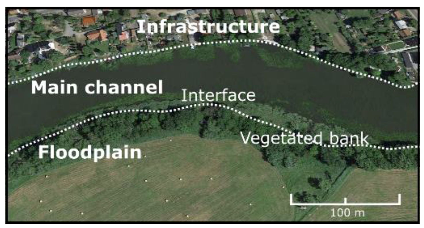
In typical main channel—a floodplain setting (e.g., Figure 1), the increased turbulent intensities at the interface region affect sediment transport mechanisms and the ratio of sediments moving in suspension; e.g., [5]. Therefore, the interface region is of major importance, as it controls the lateral transport of suspended sediment (SS) and net deposition in the vegetated areas. Maintenance of the floodplain/riverbank vegetation provides means not only to enhance flow conveyance and prevent excessive flooding, e.g., [6] but also to control SS transport and net deposition [4,7]. Important advances in the mean flow and the turbulent flow fields were gained in partly vegetated flumes by assuming plants behave as rigid cylinders; e.g., [8,9]. The drag induced by rigid cylinders is a function of the cylinder Reynolds number ReD defined as: , where U is the streamwise velocity, D the cylinder diameter, and ν the kinematic fluid viscosity. However, in nature, plants are often non-cylindrical, consist of majorly flexible material, and their properties vary both spatially and temporally; for example, due to growth, decay, and shedding of leaves. Properties such as the height, density, and flexibility of the vegetation affect lateral flow interactions; e.g., [7,10]. This calls for accounting for the flexibility-induced reconfiguration and foliation [7,11]. However, in common practice, the drag induced by the foliation and flexibility is calibrated by adjusting the stem density N (stems m−2), diameter D, and drag coefficient CD, which lacks physical meaning and interpretation. The effects of plant flexibility such as bending and reconfiguration on the vegetated drag, have been investigated for grasses [12] and for shrubs and other woody plants [7,13,14]. However, the effect of flexible vegetation and foliage on SS transport remains less researched. Previous studies showed that flexible elements controlled the flow velocity and turbulent intensities [15,16,17], and we, consequently, expect it to influence the distribution of suspended sediment and net deposition, as in [11,18].
Research addressing a mixture of transport modes, including bed-load, sheet flow, and suspended sediment transport are rare; e.g., [7]. Existing methods for estimating the bed shear-stresses are unsuitable for positions in or near the vegetated areas because of alterations of the near- bed velocities and turbulence intensities by the vegetation [16,19]. To advance the understanding of the transport, mixing, and deposition of suspended sediment at vegetated interfaces, reliable data on the spatially varying concentrations and insight on the transport mechanisms and processes are needed [5,20]. Recent experiences indicate that the spatial and temporal variations of concentration can be measured with good accuracy by means of optical or acoustic sensors in controlled flume environments [21,22,23]. The omnidirectional fluctuating component of the concentration induced by turbulent motions can be derived from the concentration time-series [23]. Optical backscatter sensors provide means to quantify the turbulent sediment diffusion coefficients and analyze its spatial and temporal variability for positions in and near the vegetated areas.
Some studies were able to explain patterns of concentration and net deposition based on the mean flow distribution and flow characteristics [8,9,24,25], whereas others explained the distribution of concentration, including the complex but relevant turbulent flow characteristics [5,26,27,28]. To the authors’ knowledge, only a few studies, e.g., [7,29], have related deposition to hydraulically sound properties of complex riparian vegetation. Laboratory or field studies on a combination of the flow field, sediment concentrations, and net deposition are rare because collecting these data with high-spatial-resolution is time-consuming and tedious. Further, the flow-vegetation-sediment phenomena and processes are numerous, which require detailed descriptions and careful consideration in modelling approaches.
The purpose of this study was to investigate the interplay between the flow field, concentration, and net deposition of fine, sandy, suspended sediment in a partly vegetated channel under leafless and foliated conditions with medium to high mean bulk flow velocities. The specific objectives were to:
- (i)
- Characterize the mean and turbulent flow field at the lateral interface between the unvegetated (UP) and vegetated parts (VP) of the channel to support analyses on suspended sediment transport and lateral mixing. We aimed to provide insights on sediment transport and mixing efficiencies by linking the velocity differences with the drag induced by the vegetation.
- (ii)
- Quantify the vertical and lateral distribution of suspended sediment concentration in the unvegetated, vegetated, and interfacial region of the flow. The linkage between the flow velocities and turbulence intensities with the suspended sediment concentration (SSC) provide the means to explain the distributions of SSC and sediment transport.
- (iii)
- Quantify net deposition in the vegetated areas of the channel considering its spatial variability. This provides insights in both the longitudinal and lateral components patterns of net deposition, which is related to the vegetation densities.
Flow field data were collected by acoustic Doppler velocimetry (ADV), suspended sediment concentrations by optical backscatter sensors, and net deposition by a weight-based approach. Data were collected in an experimental flume mimicking a main channel with a vegetated bank consisting of understory grasses and emergent flexible woody vegetation. Measurements conducted in this study were collected in parallel with a study on the turbulent flow induced by flexible vegetation between the main channel-floodplain interface [30]. Those data and analyses for example on the horizontal moving coherent flow structures support the explanations on the suspended sediment transport and net deposition given in the present study.
Experimental runs were conducted for two vegetated conditions representing seasonal differences: leafless and fol iated woody plants with dense understory grasses, under medium (MQ) and high flow rates (HQ) at bulk mean flow velocities of Um = 0.49 m/s and Um = 0.82 m/s, respectively. Those flow velocities correspond to typical values for partly vegetated rivers or streams under flood-flow conditions [24], where the transport mode of fine sand fluctuates from bed-load to SS load. The scope of the present study was limited to the non-cohesive SS transport processes and sedimentation in the vegetated areas of the channel.
2. Materials and Methods
2.1. Experimental Conditions
Experiments were conducted at the Aalto Environmental Hydraulics Lab (Espoo, Finland) in the 20 m long Environmental Hydraulics Flow Channel, which is specifically designed to recirculate fine sediment. The glass-walled working section of the tilting flume is 16 m long and 0.6 m wide. A conceptualization of the experimental flume setting for the leafless and foliated vegetation test cases is shown in Figure 2. The water depth h was kept constant at 0.17 m by adjusting the weir at the downstream end of the flume. All experimental runs were conducted in steady and quasi-uniform flow conditions. The discharge was measured by an electromagnetic flow-meter (DN150 Endress Hauser) at an accuracy of ±0.5%. Water depths were measured by six pressure transducers (accuracy ± 3 mm) distributed along the centerline of the flume. All these data were recorded at 20 Hz. Table 1 summarizes the conditions of the four experimental runs where leafless (L) and foliated (F) conditions were investigated at medium (MQ) and high (HQ) flow rates.
Sediments were fed upstream of the channel (at x = −1.75 m, Figure 2) with a constant rate of 2.3 g/s using a specifically designed sediment feeding system. The system consisted of a sediment container and a rotational screw driven by an electric motor, allowing for an adjustable feeding rate depending on the rotation frequency. The sediments were equally distributed over the flume width W using a conical shaped plate and were dropped in the water from ~25 cm above the water surface. Due to sediment feeding from the top of the water surface, the vertical profile of SS concentration was still developing in the region before entering the vegetated cross-section. Twelve point-measurements of the concentration spread over the cross-section at x = −1 m showed an equal distribution. It was expected that shortly downstream of the leading edge, the vegetation setup would dominate the flow field and SSC profiles.
The aspect ratio W/h in the present study was 3.5 as a compromise between the scaling of vegetation, realistic vegetation properties, and flow depth required for accurate measurements. Potentially, secondary flow structures induced by the walls could influence the flow field over the entire width of the flume, which typically results in an inflection point of the streamwise flow velocities close to the surface [32]. In the present experimental runs, the secondary motions induced by the walls were expected to be of minor importance compared to the modification of the flow by the vegetation.
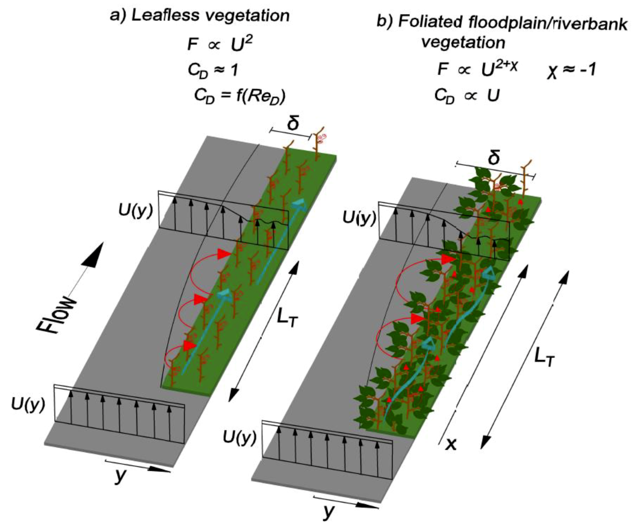
There are notable differences in the description of the lateral mixing layer between rigid and flexible foliated vegetation caused, for example, by the lateral waving of the vegetated interfaces [30]. Leafless plant stems can be considered rigid cylinders and parameterized following a rigid cylinder model; e.g., [2,3,8,9]. Flexible, foliated floodplain vegetation has been modelled through approaches taking into account the reconfiguration and streamlining, e.g., [7,30]. In the rigid cylinder case, the drag force is assumed to scale with the velocity squared , whereas in the flexible case, the drag force scales with , where χ is the reconfiguration parameter which is species-specific [7,14]. The advanced parameterization by [7] allows explicitly considering both leafless and foliated states.
2.2. Vegetated Cross-Section and Characteristics
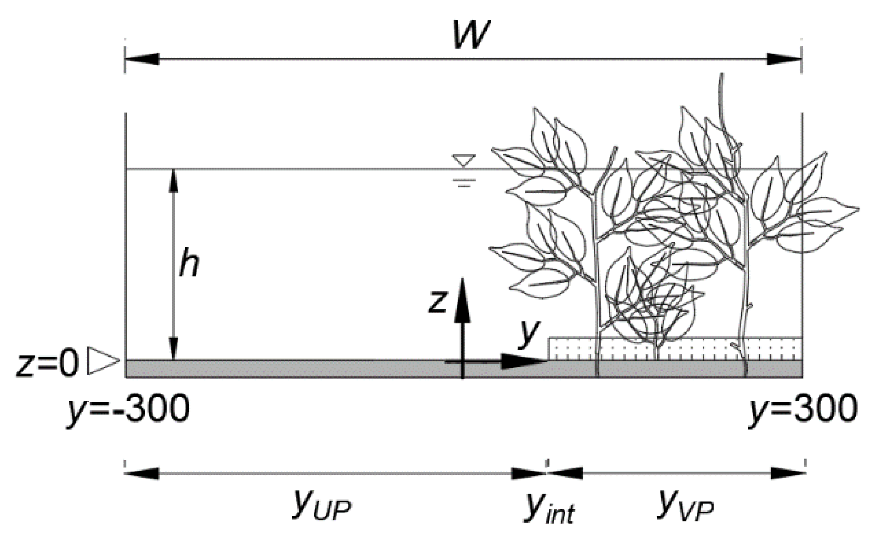
A combination of submerged grasses and emergent woody vegetation was selected, mimicking a natural-like vegetated bank with similar flexibility and reconfiguration as riparian vegetation. The vegetated area was 10 m in length and 0.23 m in width and was installed 4 m downstream of the start of the working section (Figure 2). In our left-handed coordinate system, x = 0 was at the upstream edge of the vegetation, y = 0, the centerline of the 0.6 m wide flume, and z = 0, the bed. Figure 3 shows a conceptual cross-sectional view of the channel with the unvegetated (UP) (−300 < y < 70 mm) and vegetated parts (VP) (70 < y < 300 mm). The bottom grasses were on average 20 mm tall and consisted of 0.8 mm wide stems with a uniform stem density of ~65 stems/cm2. The woody flexible plants were on average 17 cm tall and had a stem diameter of 3.3 mm, with a frontal projected stem area per unit bed area of 0.02 m2/m2 and a corresponding reference area per unit water volume of 0.13 m−1. In the foliated conditions, leaves were present in clusters of four with an average one-sided leaf area per unit bed area of 0.7 m2/m2 and a corresponding reference area per unit water volume of 4.1 m−1 (Table 1). In the MQ flow conditions, bending of the stems was minimal, while reconfiguration of the foliage was observed. In the HQ flow conditions, the foliated plant stems were bent and the leaves strongly reconfigured. The vegetation drag-density parameter CDa was 0.205 and 0.181 for the leafless MQ-L and HQ-L cases, and 1.432 and 0.485 for the foliated MQ-F and HQ-F cases, respectively [30]. The total drag density induced by the vegetation was computed from a momentum balance, deep within the vegetation [30]. The bed drag Cf was defined from the momentum balance in the unvegetated part as [33], and was 0.015, 0.021, 0.012, and 0.017 for the MQ-L, MQ-F, HQ-L, and HQ-F conditions, where g is the gravitational constant, S the slope-gradient, h the water depth, and UUP the cross-sectionally averaged streamwise velocity in the unvegetated part of the channel.
2.3. Instantaneous Flow Velocities and Turbulence Characteristics
The flow field was determined in the fully developed part of the vegetated area by acoustic Doppler velocimeters (ADVs), Nortek Vectrino+ (see details in [30]). Down and side-looking ADV probes were used to obtain data close to the bed and flume walls. Measurements collected in a region of 100 mm next to the flume walls (y < −185 mm and y > 250 mm) were excluded from the figures due to the influences of the flume walls on the flow field. Data in the dense bottom grass was collected after clearing the grass stems from a circular area with a diameter of ca. 10 mm. Each ADV measurement was conducted at a frequency of 200 Hz for a duration of 120 s. The Velocity Signal Analyser software [34] was used to filter out data with a signal-to-noise ratio <17 and to de-spike the dataset using the modified phase-space threshold method [35]. Vertical profiles were taken in the unvegetated part (at y = −150 mm), the interface region (at y = 0 mm), and in the vegetated part of the channel (at 130 mm). Lateral transects at the relative depth of 0.6 h (z = 95 mm) were taken to characterize the lateral shear layer formed between the unvegetated and the vegetated part of the channel.
To characterize the mean and turbulent flow, the following parameters were computed: the mean streamwise velocity U, turbulent kinetic energy k, turbulence intensity I, and lateral Reynolds stress τxy. The point time-averaged streamwise velocity , was calculated as: , where n is the number of instantaneous streamwise velocities measured. The turbulent kinetic energy k, was calculated as: where , and are the mean instantaneous deviations from the mean horizontal u, lateral v, and vertical w velocities, respectively, with the overbar denoting time-averaging. The total turbulence intensity I, was calculated as: .
2.4. Sediments: Physical Properties, Suspended Sediment Concentrations, and Transport
2.4.1. Physical Sediment Properties: Size, Shape, Specific Gravity, and Fall Velocities
Natural silica quartz with a narrow particle size distribution (PSD) was selected to ensure that the sediment was transported as individual particles not exhibiting cohesive behavior, to ensure uniform grain size distribution in all experiments. According to the manufacturer, the Sibelco S90 sand consists of silicate oxide (SiO2); the particles are flat-to-angular shaped and have a solid density, ρp of 2.65 g/cm3, and a dry bulk density of 1.4 g/cm3. 99.9% of the particles were larger than 63 µm, 2.9% within 63–90 µm, 87% within 90–180 µm and 10% within 180–250 µm. The median diameter (d50) of the particles was 150 µm, the d10 and the d90 were 110 and 160 µm, respectively. Corresponding settling velocities ws were estimated; ws10 = 0.011, ws50 = 0.015, and ws90 = 0.017 m/s for the d10, d50, and d90 sized particles, respectively. These estimates were derived using a force balance approach in combination with Stokes’ law, following a published approach [36], with particle Reynolds number Rep ranging between 3.6 and 5.2. The PSD of the sediment was considered reasonable for representing transport processes in vegetated lowland channels at medium to high flow conditions where suspended transport dominates.
2.4.2. Sediment Transport Modes and Mechanisms
Sediment transport modes and mechanisms vary both spatially over the channel cross-section [5] and temporally in natural rivers and streams. The onset and rates of sediment transport are commonly related to the bed shear stress τb [19,37]. The bed shear velocities in the unvegetated parts of the channel (at x > LT, y = 0 mm, z = 5 mm, Figure 3), defined as: , ranged between 0.04 and 0.07 m/s for the MQ-L, MQ-F, HQ-L, and HQ-F conditions. Sediments transported in the unvegetated channel part remained in motion and the bed-load was absent in the HQ conditions, while in the MQ cases, the formations, movements, and interactions with the SSC of crescent-shaped dunes were observed. The vertical mixing efficiencies between the near-bed region and upper layer relates to the bed shear velocities in combination with the near-bed turbulence. In the current experiments, the importance of the bed load compared to the SS load was assumed to be of minor importance. The Rouse number, Ro, defined as: Ro = ws/κ, where κ is the von Kármán coefficient was 1.02, 0.83, 0.59, and 0.54 at the center (at x > LT, y = 0 mm, Figure 3) of the lateral cross-section for the experimental runs MQ-L, MQ-F, HQ-L, and HQ-F, respectively. These low values of Ro suggest that the majority of the sediments were transported in suspension [36], following SS transport mechanisms and processes solely. For the unvegetated part of the channel, the proportion of the near-bed load (z/h < 0.15) compared to the SS load (z/h > 0.15) was estimated from both SSC measurements and measurement with a down-scaled Helley–Smith type bed-load sampler. The estimated proportion of the near-bed flux ranged between 17% and 23% for the tested experimental conditions. In the vegetated parts of the channel, sediment transport in the near-bed region (z > 20 mm, Figure 3) was absent as the result of the low flow velocities and turbulence intensities caused by the dense bottom grasses.
2.4.3. Suspended Sediment Concentration by Optical Backscatter Techniques
SSCs were measured with three Campbell OBS−3+ optical backscatter sensors (OBS). The sensors were calibrated in the flume for five intervals of increasing concentration ranging from ~10 to 300 mg/L, while flow and light conditions were kept constant, as in [38]. The sensors exhibited high linearity and correlations (r2 = 0.96) between the sensor output in voltage (V) and SSC [38]. The sensors were configured to measure at a rate of 10 Hz, with a manufacturer-stated accuracy of 4% or 10 mg/L for sandy material. The sensors were placed, with the optics facing the upstream flow direction with at least 10 cm distance between the sensor optics and vegetation elements to avoid protrusions of the sample volume. Near the bed (z ≤ 25 mm), concentrations showed larger variability due to the disturbances in the sampling volume for example by bed reflections. Largely disturbed measurements by the vegetation or the bed reflections were omitted in further analyses and excluded from the figures.
Lateral profiles of one-minute duration point measurements were taken at a relative depth of 0.6 h, and vertical profiles were taken over 10 < z < 145 mm and 25 < z < 145 mm for the open and vegetated part of the channel, respectively. The reference concentration at the start of the experimental runs C0 (t = 0) was ~20 mg/L. The reference concentration Cref(t) was continuously recorded at x = 4 m, y = 0, and z = 95 mm. Cref(t) increased over time in the experimental runs because of the recirculation of sediments back into the inlet and the constant feeding of sediments. The SSCs that were measured were scaled by C0 to allow comparisons between points in the collected profiles (as explained in Appendix A). The fluctuating component of the measured SSCs’ IC was calculated from the time series of instantaneous concentrations as the square root of the time-averaged squared fluctuation of the concentration divided by the time-averaged concentration as: .
2.4.4. Net Deposition in the Vegetated Areas
Net deposition in the vegetative areas was measured by a weight-based sampling approach from 32 removable rectangular grassed strips, with a surface area of 0.11 m2 distributed over the vegetated area. The average net deposition per unit area m was based on the three replicate runs. The spatially-averaged net deposition was calculated by spatial interpolation, taking into account the representative area of the measurement strips. The 32 measurements allowed for both longitudinal and lateral profiles of net deposition with good repeatability, despite the complex flow structures and vegetative setting. The coefficient of variation (CV) between the three replicate measurements ranged between 1% and 30%. Small differences in the initial conditions, such as the initial concentration C0, placement of the measurement strips, and the reconfiguration and dynamic motions of the flexible vegetation, are likely the major causes for the deviations between replicate measurements. For the lateral patterns, net deposition was related to the distance from the interface (y − yint, Figure 3), and scaled well with the drag density parameter CDαH to express the influence of the vegetated drag on the observed lateral patterns.
Downstream deposition affected upstream concentrations as a result of the re-circulating flow; i.e., outflow being pumped back to the flume inlet. To allow for comparing the different runs, the relative deposition was estimated as: , where Aveg is the total bed area of the vegetation, and the time-averaged reference SS flux at the reference location (x/h = 0 m, y = 0 and z = 95 mm, Figure 2). was obtained by multiplying the discharge Q by the time-averaged reference concentration . The SS fluxes qss over the unvegetated qss,UP and vegetated cross-sections qss,VP of the channel were estimated as: , where A is the cross-sectional flow area of the considered cross-section.
2.4.5. Describing Laterally and Vertically Suspended Sediment Transport in Vegetated Mixing Layers
In the absence of lateral advection, laterally suspended sediment transport is generally driven by mechanical dispersion, turbulent diffusion, and molecular diffusion [8,26,33]. Molecular diffusion can be neglected in conditions with a strong shear layer where mixing by mechanical dispersion and turbulent diffusion dominates. In partly vegetated flows with a strong shear layer, lateral mixing depends on the magnitude, size, and frequency of the horizontal moving vortices [33]. The importance of turbulent transport on lateral mixing is expressed as the ratio τxy/k, i.e., [33].
In this study, we proposed the use of the differential SSC λc as an indicator of the integrated effect of lateral mixing and net deposition on the lateral SSC distribution across the mixing layer. Analogously to the characteristic properties of flow in mixing layers [31], the differential SSC was calculated as λc = ([CUP − CVP]/[CUP + CVP]) where CUP and CVP are the spatially averaged concentrations of the UP and VP at a relative depth of 0.6 h, respectively. For the foliated partly vegetated channel, ∆C between the UP and VP depends on the drag ratio λd between the vegetated and unvegetated parts as: where Cf is the bed drag coefficient of the channel. The drag ratio was defined analogously to the differential velocity of the shear layer, considering the areas outside of the region where shear stresses are large. Thus, in the vegetated part, the drag caused by the vegetation dominates while bed friction is negligible, whereas in the unvegetated areas, bed friction dominates and vegetative drag is absent.
Vertical profiles of SSC are commonly described by a modified form of the Rouse equation which, is derived by expressing the vertical mixing coefficient, and solving for the concentration C and depth z [39] as: , where Ca is the sediment concentration at the reference elevation za. For the upper region of the flow depth z/h ≥ 0.5, van Rijn [40] proposed a modified form of the Rouse equation: . In the present study, za was based on the lowest measurement taken at z = 10 mm.
3. Results and Discussion
3.1. Lateral Distributions of Key Flow Parameters, SSC, and Net Deposition in the Fully Developed Flow Region
Lateral distributions of the flow and turbulent flow field are shown in Figure 4 and Figure 5. These figures support the indication of the effects of the bulk flow velocity and the presence of foliage on the lateral distributions.
3.1.1. Mean Flow Velocity and Turbulent Flow Characteristics
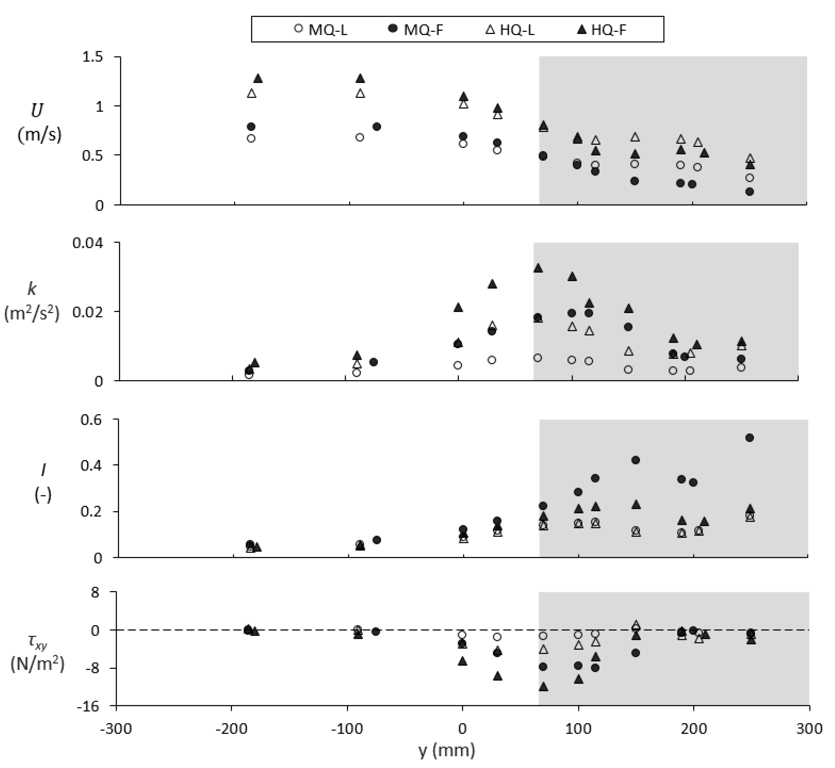
Figure 4 shows the lateral distribution of the mean streamwise flow velocity U, turbulent kinetic energy k, turbulence intensity I, and lateral Reynolds stress τxy at the relative depth of 0.6 h (z = 95 mm). The lateral flow fields indicated a typical mixing-layer type flow with a strong velocity gradient ∆U between the interface and vegetation, ranging between 0.27 and 0.74 m/s (Table 1). This resulted in a strong shear layer with high lateral Reynolds stresses τxy at the interface, ranging from −1.37 to −11.98 N/m2. U was highest in the unvegetated part, decreased over the interface, and was lowest in the vegetated part of the channel. This strong velocity gradient is often present in channels differing in vegetative drag and roughness [2,3]. The turbulent kinetic energy and the turbulence intensities were highest at the interface (0.007–0.034 m2/s2) and remained relatively high throughout the vegetated part compared to the unvegetated part outside the shear layer, especially in the foliated conditions. k decreased for positions of increasing distance from the interface while remaining relatively high in the vegetated part compared to the unvegetated part, especially for the foliated conditions. I increased over the interface and was about two times higher in vegetated part compared to the part of the unvegetated channel located outside the lateral shear layer, at y < −100 mm. τxy was largest at the interface between the vegetated and unvegetated part of the channel, was about three times higher for the foliated conditions compared to the leafless conditions, and was about two times higher for the high-flow rate compared to the low-flow rate. The streamwise flow velocities were on average 2.4 times lower in the vegetated part compared to the unvegetated part, while k was about two times larger and I was 3–4 times higher. In the present study τxy/k ranged between 0.22−0.25 and 0.38−0.43 at the interface (yint = 70 mm) for the leafless conditions and the foliated conditions, respectively. These relatively high values of τxy/k suggest a strong influence of the turbulent flow component on the lateral movements of suspended sediment [3].
The woody plants generated turbulence at the plant-stem scale, visible as high turbulence intensity directly downstream of the stems (at y = 125 mm and y = 250 mm in Figure 4). The presence of foliage caused the turbulent kinetic energy to increase by two to three-fold in the interface region and in the vegetated areas of the cross-section (Figure 4). This is the result of the turbulent kinetic energy generated by the flexibility of the plants stems and leaves [10,41].
3.1.2. Lateral Variation of Suspended Sediment Concentration and Fluctuation Component IC
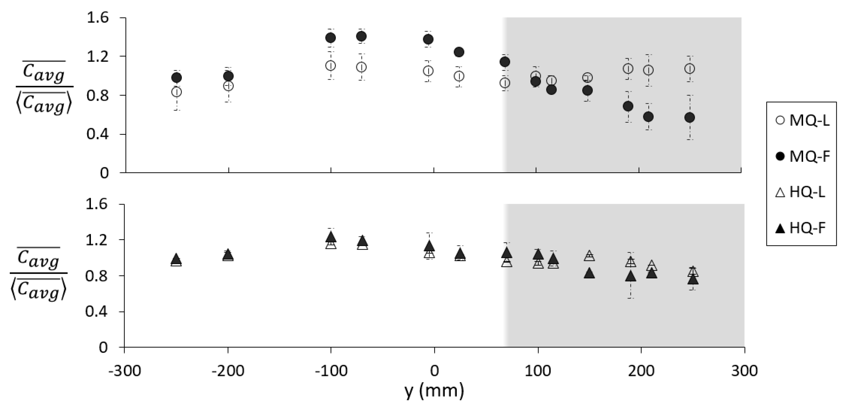
Figure 5 shows the time-averaged concentration obtained from the 60 s measurements with the calibrated OBS sensors normalized with the spatial-averaged concentration at the relative depth of 0.6 h, and the standard deviation computed from the two replicate measurements in the fully developed flow region at x/h = 68. In the medium flow rate, was 88 and 113 mg/L for the leafless and foliated conditions, respectively. For the HQ conditions was 90 and 87 mg/L for the leafless and foliated conditions, respectively. was highest in the unvegetated part of the channel (at y ≈ −90 mm) and decreased over the interface between the unvegetated and vegetated parts. Concentrations were at their lowest in the vegetated part furthest from the interface. The exception was the leafless run at MQ, where the concentration was about equal over the entire cross-section. The largest lateral gradient of concentration (∂C/∂y) over the interface was observed for the MQ-F condition. This suggests a strong effect of the foliation on the lateral distribution of the concentration. The decrease in concentration observed for locations near the flume wall (y < −200 mm) were likely the result of the flume wall effects, related to the reduction in flow velocity (Figure 4 and Figure 5).
The intensity of the fluctuation component of SSC (IC) over the lateral cross-section at the relative depth of 0.6 h is shown in Figure 6. The cross-sectional averaged IC was 2–3 times lower in leafless (0.037–0.038) compared to foliated conditions (0.10–0.13). was highest for the MQ with foliated conditions. In the leafless conditions, the IC was higher in the UP compared to the VP. For the foliated conditions, the IC remained relatively high over the entire width of the vegetated part for the MQ, while it showed a marked decrease with increasing distance from the interface (y > 150 mm) for the HQ. Overall, IC had higher, non-systematic spatial variability within foliated compared to leafless vegetation, which was expected to be generated by the presence of foliage.
3.1.3. Characterizing the Lateral Distribution of Suspended Sediment Concentration in the Vegetated Mixing Layer
Table 2 shows the laterally averaged concentration in mg/L in the unvegetated (UP) and vegetated (VP) parts of the channel and the concentration difference ∆C between the UP (CUP) and VP (CVP). In the MQ, was approximately equal between VP and UP under leafless conditions, while it was approximately three times lower in the VP compared to the UP under foliated conditions. In the HQ conditions, remained relatively high in the vegetated part of the cross-section and was 13% and 22% lower in the VP compared to the UP for the leafless and foliated conditions, respectively. Thus, the concentration difference ∆ was highest for the foliated condition in combination of the MQ.
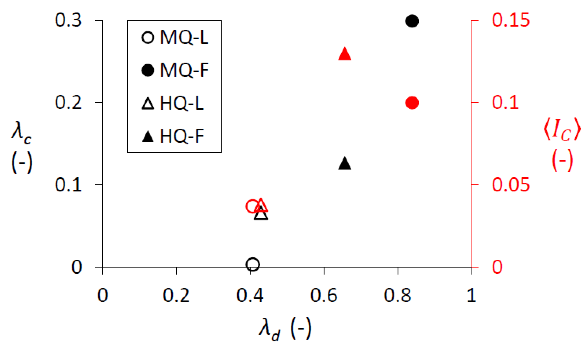
The differential concentration ∆C (CUP − CVP) between the UP and VP of the channel relates to the drag density CDaH induced by the vegetation. The results showed that λc ([CUP − CVP]/[CUP + CVP]) increased for larger CDaH (see Table 2 and Figure 7). Linkage of ∆C to the drag difference between the UP and VP provides insight on the lateral distribution of the suspended sediment concentration and mixing efficiencies. MQ = medium flow rate (50 L/s); HQ = high flow rate (83 L/s); L = leafless; F = foliated.
The differential concentration λc and laterally averaged fluctuating component increased for an increasing ratio of the vegetation-induced drag differential λd ([CDaH − Cf]/[CDaH + Cf]) between the unvegetated and vegetated part of the channel (Figure 7). This shows the potential of λc as an indicator for the integrated effect of lateral mixing of SS between the unvegetated and vegetated channel parts and net deposition within the vegetated areas. This provides the means for quick estimates on the lateral exchange rates based on the drag-ratio between the UP and VP of the channel. To indicate the limitations of the predictive capabilities of the drag-ratio, further insights are needed on the concentration differences and mixing efficiencies in relation to the density of the vegetation, and vegetative drag.
3.1.4. Lateral Patterns of Net Deposition in the Fully Developed Flow Region (x > LT)
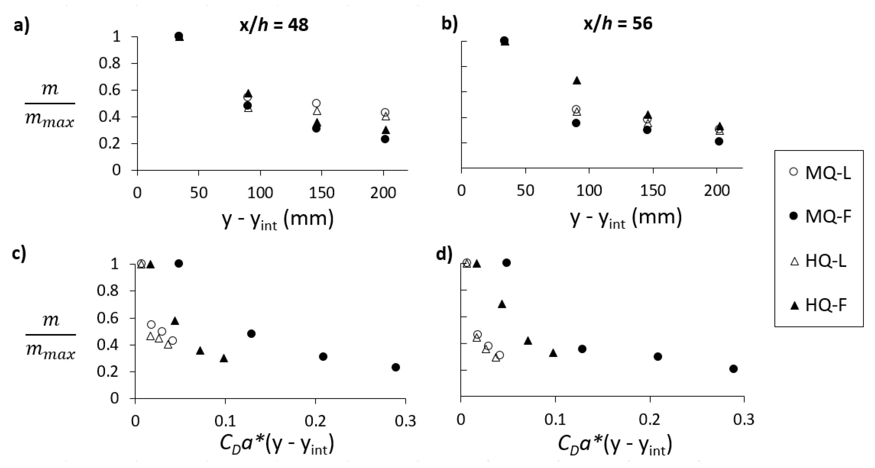
Figure 8 shows the lateral pattern of net deposition m over the vegetated area (yVP) normalized with the maximum net deposition mmax. These cross-sections are located in the fully developed flow region (x > LT). Net deposition near the interface (at y − yint = 34 mm) was about two to five times higher compared to net deposition for positions of larger distances from the interface. The strongest lateral gradient of net deposition was observed for the MQ-F run. For most locations over the longitude, was larger for the foliated condition compared to the leafless condition (see Figure 8). The presence of foliage enhanced net deposition (scaled by the time-averaged SS flux ) at the lateral edge by five times for the MQ condition, while for the HQ condition, net deposition at the lateral edge remained about equal. For positions of larger distance from the interface (e.g., at dy = 202 mm) net deposition was two times higher in the MQ-F condition.
Figure 8c,d shows that the lateral patterns of net deposition scaled reasonably well with the drag induced by the vegetation when the leafless and foliated seasons were considered separately. This indicates the predictive capability of the drag density parameter CDa on net deposition near the interface of the vegetated areas.
In contrast to the present observations, the absence of net deposition near the main channel–vegetation interface has been reported, particularly when using rigid cylinders to represent vegetation [8,9,28]. The vegetated areas in those studies consisted of bare bed conditions, allowing turbulent structures to penetrate at the bed in the interface region, causing sediments to remain in suspension, or resuspension of deposited sediments at the main channel–vegetation interface. In nature, the bed is often covered with understory grasses, roots, and plant debris or a mixture of these. That suggests the necessity for improvements in the representation and characterization of natural-like river bank/floodplain vegetation, considering the complex near-bed conditions.
3.2. Vertical Distributions of the Key Flow Parameters and SSC in the Fully Developed Flow Region
Vertical profiles of the flow and turbulent field and suspended sediment concentrations are shown in Figure 9 and Figure 10. The effects of bulk flow velocity and the presence of vegetation, including foliage on the vertical distributions, are discussed in this section.
3.2.1. Vertical Profiles of the Time-Averaged Flow Velocity u and Turbulent Flow Characteristics
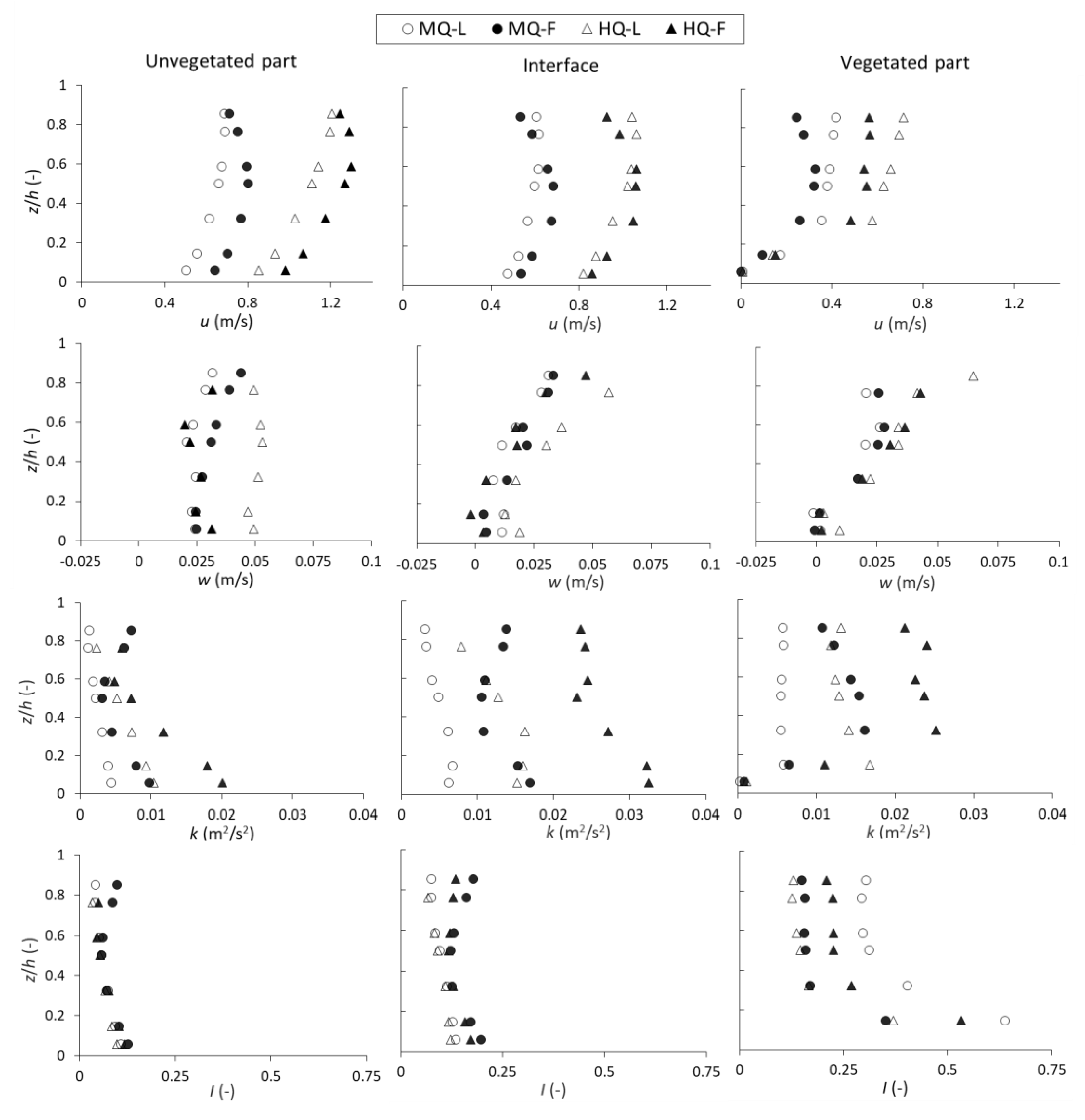
The vertical distribution of the mean time-averaged flow velocity u, turbulent kinetic energy k, and turbulence intensity I at three lateral positions are shown in Figure 9, representing the UP (y = −150 mm), interface (y = 0 mm), and VP (y = 130 mm) of the channel. In the UP of the channel, u increased with flow depth and showed a velocity dip close to the surface for the vegetated conditions. This velocity dip close to the surface was likely the result of the small aspect ratio (W/h = 3.5) [32]. In the VP, k was highest at the bed and decreased for increasing flow depth, while I remained more uniform over depth. At the interface, u, k, and I showed similar patterns over the vertical, whereas in the UP of the channel, with absolute u values slightly lower, k and I were increased. In the VP of the channel, values close to zero were measured for u and k inside the dense grassy vegetation (z < 20 mm). The vertical velocity profile of u was relatively uniform around the middle of the water column, while k was uniformly distributed over the flow depth, and I above the vegetation showed a logarithmic increase with flow depth. Both k and I were about twice as large for the foliated conditions compared to leafless conditions. The vertical velocity w was upwardly directed for most positions and of about the same order as the particle settling velocity ws50 (Figure 9). Thus, the time-averaged flow components contributed to keeping sediments transported in suspension, both in the unvegetated and vegetated channel parts, and in the main channel–vegetation interface region.
3.2.2. Vertical Profiles of SSC
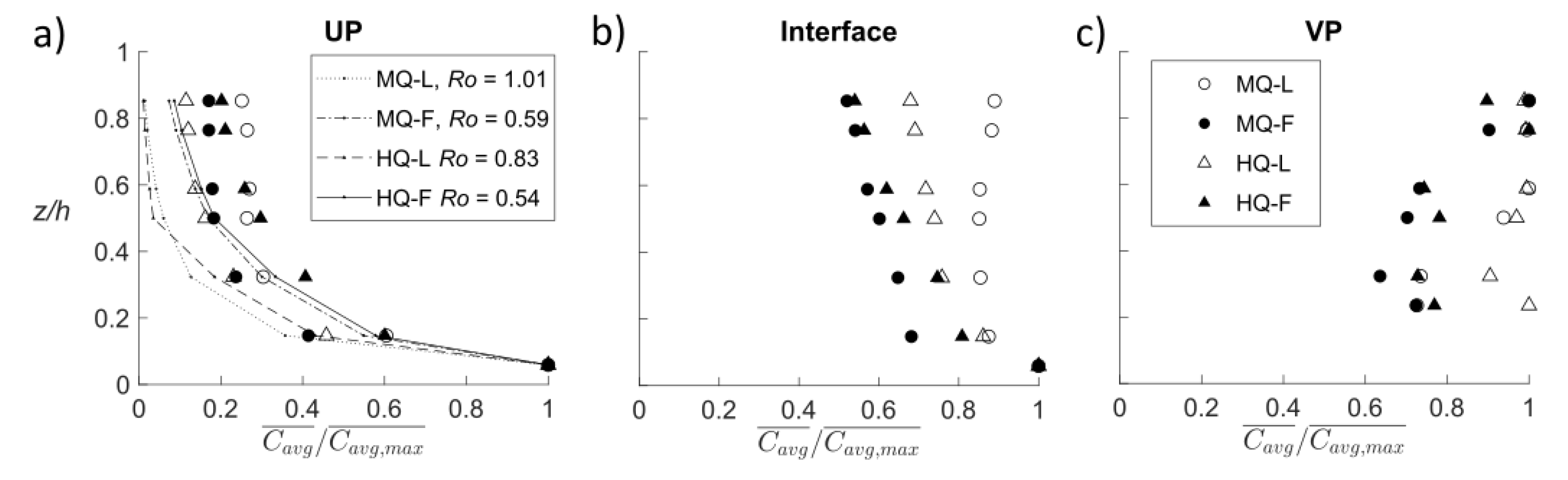
The mean time-averaged suspended sediment concentration , normalised with the maximum concentration (), of each vertical, is shown in Figure 10 for y = −150, y = 0, and y = 130 mm—representing the unvegetated, interface, and vegetated parts of the channel, respectively. The vertical profile in the unvegetated part of the channel resembles a logarithmic profile with increasing concentration for positions towards the bed. At the interface, SSC was more uniformly distributed in the vertical due to the effects caused by the vegetation. In the vegetated areas, the profiles were more complex, which can be described by a higher concentration at the top of the plants (around z/h > 0.75) and a dip in SSC in the middle of the vegetation (at z = 55 mm).
Figure 10a shows the result of the predictions of concentration based on the particle settling velocity ws and bed shear velocity in comparison to the concentration measured for the unvegetated part of the channel. The fitted profiles based on the modified Rouse equation (presented in Section 2.4.5) [40] were reasonable in explaining the vertical variation of the concentration in the unvegetated part of the channel (Figure 10a). In the region between mid-depth and the water surface (z/h > 0.5), predicted concentrations were 40% to 90% lower than measured. Deviations from the modified Rouse-profile were likely to stem from the effects of turbulence generated by the plant elements, such as the dynamic motions of the plant stems and leaves. In the main channel–vegetation interface and in the vegetated areas, the measured vertical concentration profiles deviate largely from the predictions based on the Rouse-profile. These and previous findings, e.g., [5], indicate the necessity of incorporating the effects of turbulence induced by flexible vegetation into existing analytical solutions, such as the modified Rouse equation.
3.3. Net Deposition and the Influences of Mean Bulk Flow Velocity and Foliation
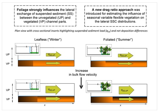
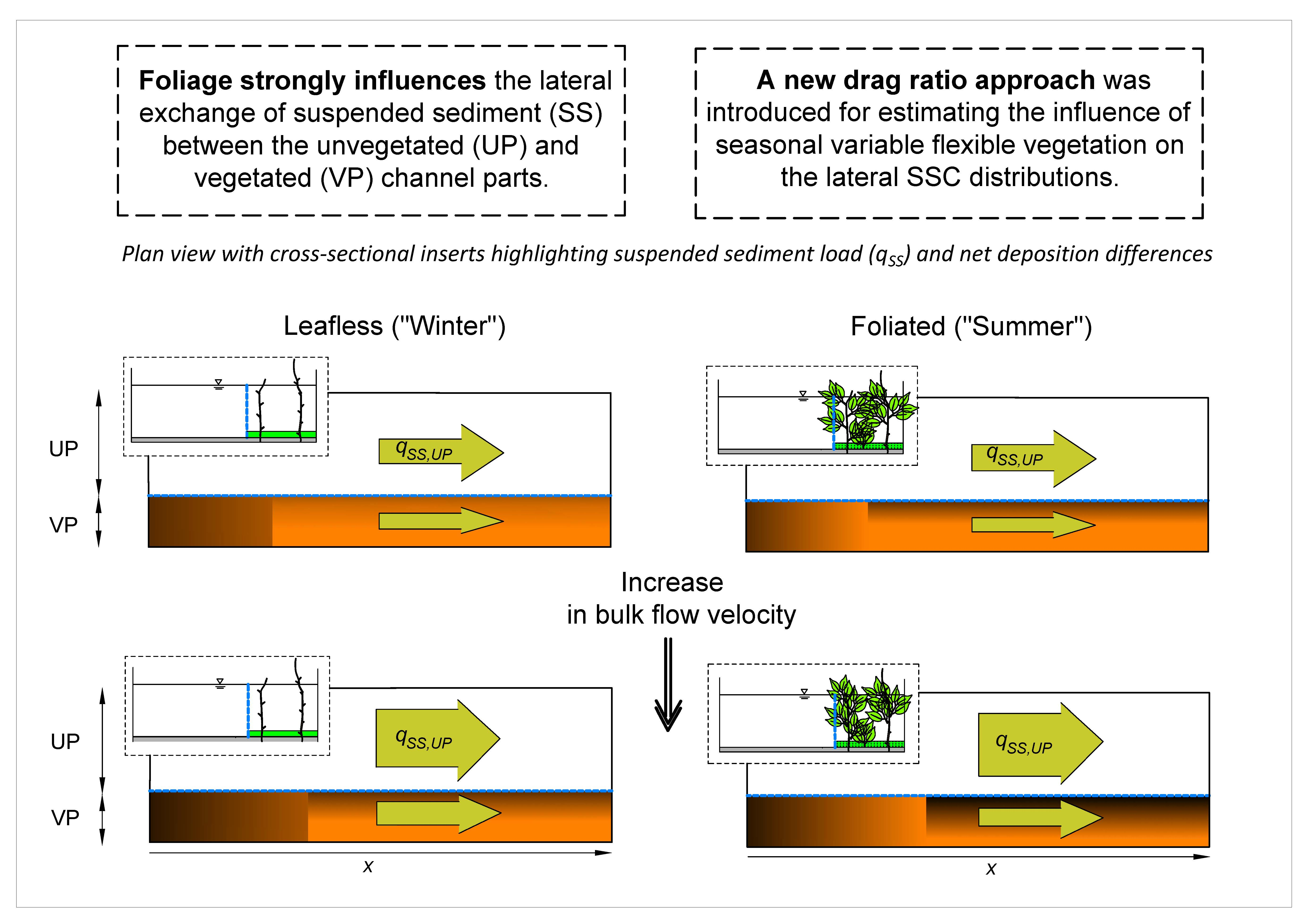
Net deposition obtained from the measurement strips in the vegetated areas provided insights on the influence of mean bulk flow velocity and foliation on both the total net deposition and patterns observed. The longitudinal and lateral patterns of net deposition are shown in Figure 11, Figure 12 and Figure 13. Results from this study were conceptualized from and are summarized in Figure 14, which provided means to discuss the influence of mean bulk flow velocity and the presence of foliage on net deposition and sediment transport.
3.3.1. Total Net Deposition
Table 3 shows the spatially-averaged net deposition per unit area with the units, mass per bed area (ML−2), in the vegetated part of the channel for the four tested conditions. The spatially-averaged net deposition was about three times higher for the high flow rate compared to the low flow rate. This is the result of the higher time-averaged SS flux for the higher flow rates (see Table 3). The share of net deposition in relation to was 11%–22%. increased by 27% and decreased by 70% for the leafless and foliated cases, respectively, by the increase of mean bulk flow velocity. The relative change in the deposition in the foliated condition compared to the leafless condition was 97% under the medium bulk flow velocities and very low (−5%) under the high bulk flow velocities (Table 3). This indicates a strong influence of the foliation, altering mixing efficiencies (Section 3.1.2) in the MQ, while in the HQ conditions, the foliage did not affect total net deposition. This can be explained by the increased contribution of longitudinal advection compared to lateral mixing of suspended sediments into the vegetated areas; and by the reduction of the strength in the lateral shear layer (i.e., indicated by the velocity ratio λ in Table 2) or magnitude, size, or frequency of the horizontal moving coherent flow structures [30].
3.3.2. Longitudinal and Lateral Patterns of Net Deposition
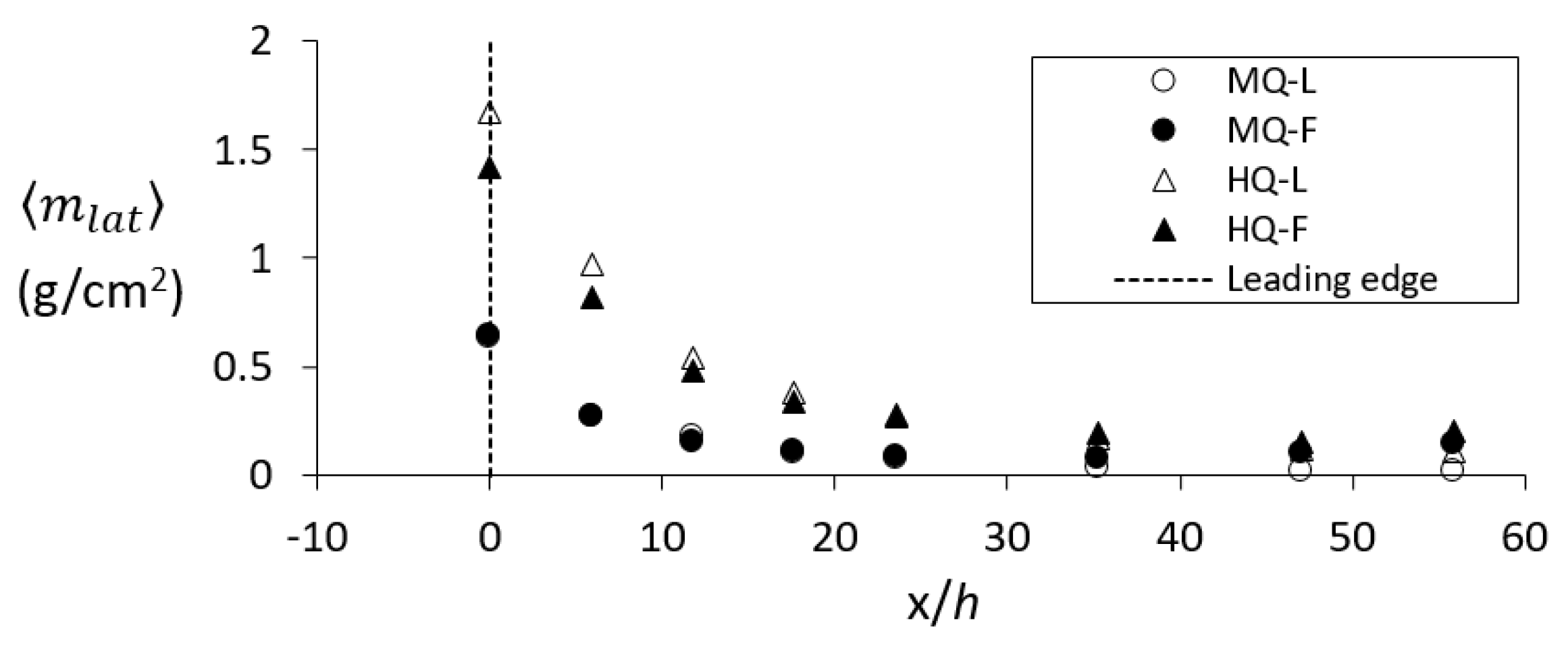
The laterally-averaged net deposition over the streamwise direction in the vegetated areas is shown in Figure 12. was four to 29 times larger at the upstream part of the vegetated area (0.64−1.7 g/cm2 at x = 0 m) compared to the downstream part (0.02−0.21 g/cm2 at x = 9.6 m). This is the result of deposition in the upstream parts reducing the sediment availability further downstream, similar to patterns observed previously [24,42]. The longitudinal gradient was largest in the diverging region of the flow (x < LT) and decreased for locations further downstream, as a result of decreasing SSC due to extensive net deposition (Figure 11).
Net deposition was roughly 2–3 times higher at the leading edge (x/h = 0) of the vegetation in the HQ conditions compared to the MQ conditions, which results from the increase in incoming sediment load (see Table 3). Bulk flow velocity has a large effect on the net deposition over the region x < LT, but of no importance in the fully developed flow region. The increase in bulk flow velocity caused the ratio of net deposition between the leading edge and fully developed region to halve for leafless conditions, while it doubled for the foliated conditions.
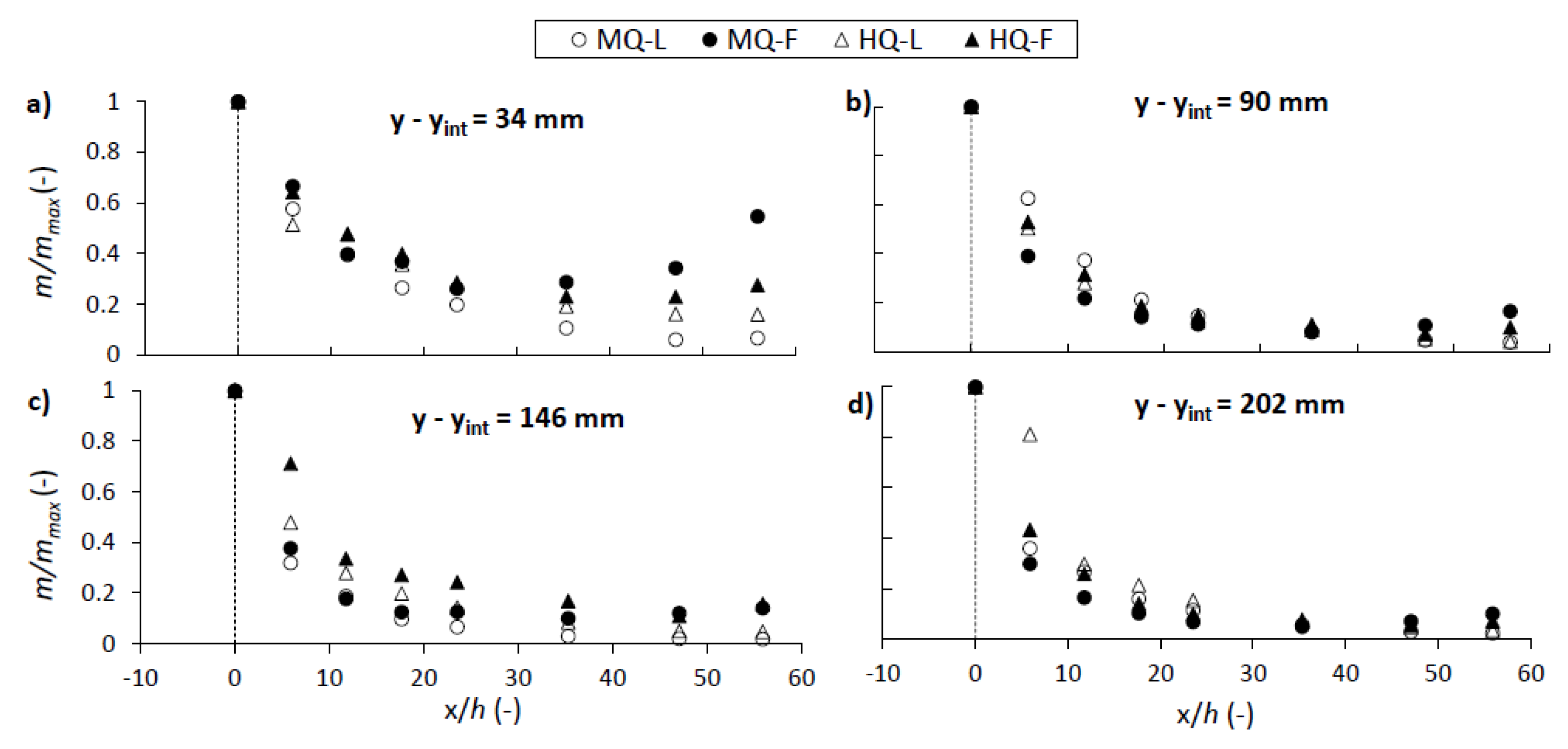
Figure 12 shows the longitudinal profiles of mean net deposition m over three replicate runs for positions of increasing distance dy (y – yint) from the main channel–vegetation interface for (a) dy = 34 mm, (b) dy = 90 mm, (c) dy = 146 mm, and (d) dy = 202 mm. Net deposition was scaled with the maximum value over the lateral mmax to allow comparisons between the experiments runs. Net deposition within vegetation decreased for increasing distance from the leading edge up to x/h ≈ 30 for all lateral positions (Figure 12). In the fully developed flow region (x > LT), net deposition remained about equal over the streamwise direction for most of the conditions. However, in the foliated conditions for positions at the lateral edge (Figure 12a), net deposition increased for positions of a larger distance from the leading edge in the region x/h ≥ 30, consistently, in the three repetitive runs. This was likely caused by the redistribution of sediments over the entire flow depth (which were preferably transported in the near-bed region in the UP of the channel in the region x/h ≤ 30) as the result of increased turbulence intensities, and of the growing size and strength of the shear layer in the streamwise direction, as observed by, e.g., [4]. The redistribution of sediments over the cross-section was expected to be strongest in the MQ-F and HQ-F conditions, having the strongest mixing layers with highest differential velocities λ (Table 1) and relatively high turbulent kinetic energy near the bed of the interface region (see Figure 5 and Figure 9). Consequently, more sediment was being transported into the vegetated areas by lateral mixing, which was assumed to enhance net deposition in the region x/h ≥ 30.
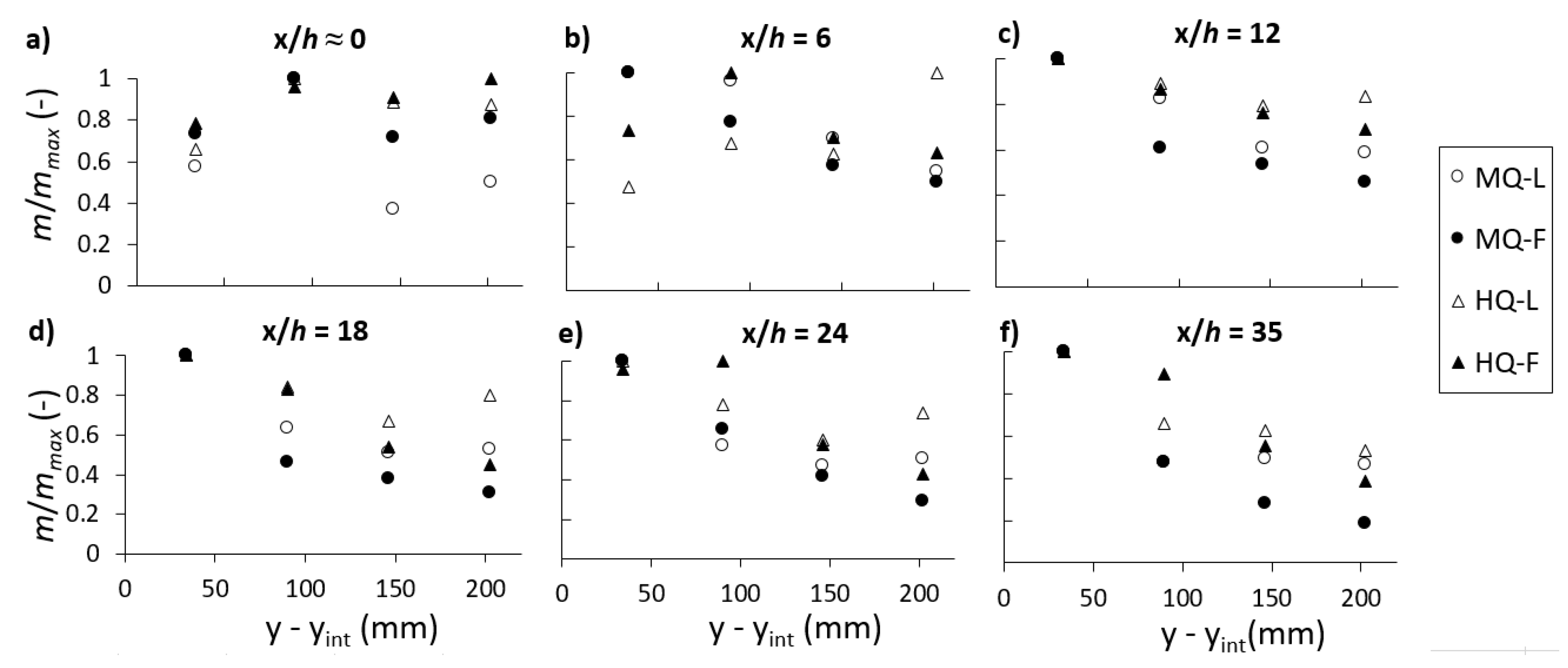
Figure 13a–f shows the lateral patterns of net deposition m normalized with the maximum net deposition over each cross-section. The typically observed lateral pattern of net deposition () of decreasing deposition for positions of larger distance from the interface developed over the streamwise direction. Large variations in the gradient were observed up to x/h = 6 in the MQ-conditions. As expected for HQ conditions, the longitudinal distance was larger, up to roughly x/h ≥ 18. That is linked to the advection length scale and the length LT of the flow development region [8]. In the fully developed region (x > LT), starting roughly from x/h ≥ ~18, the data shows a clearer trend of largest net deposition near the interface and the lowest deep within the vegetation (Figure 8 and Figure 13). This indicates the reduction of the influence of streamwise advection of sediments and the increasing importance of the lateral shear layer.
3.3.3. The Influences of Bulk Flow Velocity, the Seasonal Differences of the Vegetation, and Patch Dimensions on Sediment Transport
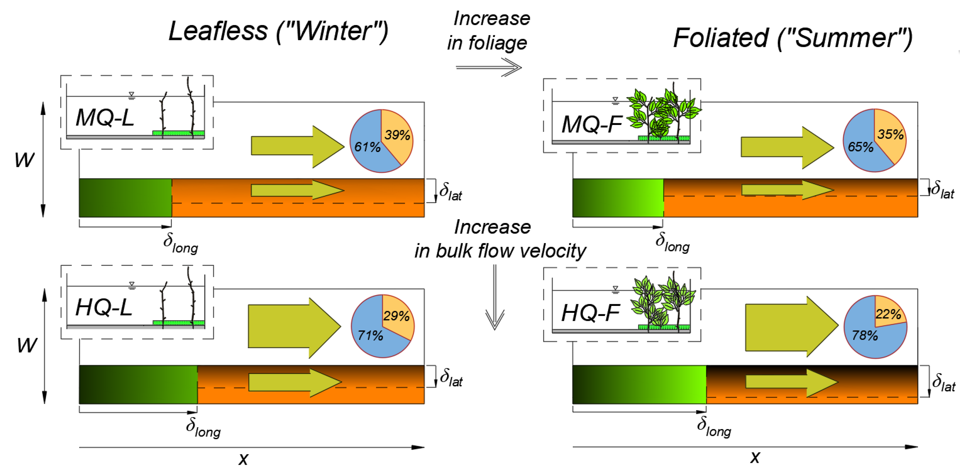
The magnitudes and patterns observed of net deposition are shown in Figure 14 for flow conditions of increasing mean bulk flow velocity (Um ~0.49–0.83 m/s) and two seasonal conditions; i.e., with and without foliage. This temporal change in foliage is one example of the many seasonal differences of natural vegetation features affecting the density, vertical structure, and flexibility. Therefore, it is beneficial to incorporate features of natural vegetation, such as the foliage and reconfiguration, towards more realistic modelling scenarios.
An estimate of the relative share of the total SS flux between the UP qss,UP and VP qss,VP of the channel is given based on paired measurements of flow and SS concentrations. The relative share of the total SS flux in the UP of the channel ranged between 61% and 78%. Both the increase in bulk flow velocity and the presence of foliage caused the relative share of the total SS flux qss to increase in the UP of the channel so that it was highest for the HQ-F condition. This can be explained by the larger increase in the streamwise flow velocities in the UP compared to the VP of the channel, with increasing discharge (Figure 4) and enhanced net deposition in the VP of the channel as a result of lateral mixing of suspended sediments into the vegetated areas. However, the lateral distance from the interface where net deposition was 40% of the maximum δlat was relatively small in the foliated condition compared to the leafless condition under medium bulk flow velocities (Figure 14). That was likely the result of particles that entered the vegetated areas from the main channel which were deposited in a narrow region at the interface, despite the increased turbulence intensities and the horizontally moving, coherent structures present.
The seasonal differences of the vegetation influenced the relative share of the streamwise SS fluxes of the unvegetated and vegetated channel parts, along with the magnitude, and longitudinal and lateral patterns of net deposition within the vegetated areas. These factors affect the downstream movement of fine sediments, and thus the annual sediment budget of a river or stream. The sedimentary budget of a main channel–vegetated floodplain setting is expected to be controlled by the flow velocity, sediment characteristics, and vegetation characteristics, with most evident impacts occurring during the high flows and late in the growing season due to dense foliage [7].
The bulk flow velocities decreased in the VP of the channel due to the vegetation-induced drag, with flow diverging from the VP to the UP near the leading edge [2,8,28]. The length of the developing region LT increased with the cross-sectional flow velocity [2,8,43], and was expected to increase with the presence of leaves through notably higher vegetative drag. In the developing region (x < LT), net deposition was the result of streamwise advection and lateral dispersion of SS, where transport by advection dominates [8]. The effect of foliage on δlong was of minor importance compared to the bulk flow velocity (Figure 14), while δlat had a stronger dependency on the vegetative drag-density ratio (Figure 8). Lateral mixing rates of SS are expected to increase for locations at a larger distance from the leading edge as a result of the increasing size, strength, and frequency of coherent structures [2,3]. Based on the results presented in this study, for long stretches (x/h > ~30) of riverbank vegetation, net deposition is driven by the size and strength of the shear layer between the main channel and vegetated channel part, which is dominated by the turbulent flow characteristics. For shorter patches (x/h < ~30) sediment transport by advection is expected to dominate deposition, while flow turbulence influences net deposition by altering particle flow paths and sediment resuspension rates. Further investigations are needed on net deposition in and behind patches of natural-like vegetation of different sizes, investigating the effects of coherent flow structures and turbulence on net deposition and transport of fine sediments in more detail; e.g., [17,37].
4. Conclusions
With the present research, we seek to improve predictions on the suspended sediment transport and deposition in partly-vegetated, main channel-floodplain/riverbank settings. An exceptional experimental campaign with foliated and leafless flexible model vegetation, itself with understory grasses, was designed so that new data were collected concurrently on three aspects: suspended sediment concentrations (SSC), net deposition, and the flow field. Most flume studies are limited to investigating only one or two of these aspects with rigid cylinder models, whereas the effects of flexible, riparian vegetation with foliage remain undescribed.
Within and near the vegetated areas, the velocity profiles and turbulence intensities were markedly modified by the vegetation, which largely affected the vertical SSC distributions. The effects on the SSC distributions were more pronounced with the foliated compared to the leafless vegetation. The foliage strongly influenced the lateral exchange of suspended sediments between the unvegetated and vegetated parts of the channel, as summarized in Figure 14. Consequently, we introduced a new drag ratio approach for estimating the influence of seasonally variable flexible vegetation on the lateral SSC distributions. The presence of foliage caused the total net deposition to increase by 97% for the medium bulk flow velocities and enhanced the deposition near the main channel-floodplain interface by two to five times.
Our research demonstrated that experiments and models on sediment transport and deposition will benefit from a more realistic representation of natural riparian vegetation that is typically composed of highly variable plant types. Common flume study arrangements with arrays of static, rigid cylinders were found to be inadequate for physical modelling of net deposition on natural floodplains, as the cylinders cannot reproduce the vertical vegetation structure, including a herbaceous understory layer.
Author Contributions
All authors, W.B., K.V., J.J. contributed to the conceptualization; W.B., was mainly responsible for the data analyses; All authors contributed significantly to the preparation and writing of the original draft; K.V., J.J. contributed to writing-review and editing.
Funding
The research was funded by Maa-ja vesitekniikan tuki ry (number 36537 and 33271) and by Maj and Tor Nessling Foundation (number 201800045).
Acknowledgments
The authors gratefully acknowledge the help of Antti Louhio and Gerardo Caroppi, Chiara Ghio, and Markku Andelin in the data collection.
Conflicts of Interest
The authors declare no conflict of interest.
List of Symbols
| Symbol | Units | Fund. Dim. | Description |
| A | m2 | L2 | cross-sectional area; |
| Aveg | m2 | L2 | vegetated surface area; |
| a | m−1 | L−1 | frontal vegetated area per unit volume; |
| aL | m−1 | L−1 | frontal projected leaf area per unit volume; |
| aS | m−1 | L−1 | frontal projected stem area per unit volume; |
| CD | - | - | drag coefficient; |
| CDa | m−1 | L−1 | vegetative drag; |
| Cf | N m−2 | ML−2 | bed drag coefficient; |
| C0 | mg L−1 | ML−3 | initial SSC; |
| Cref | mg L−1 | ML−3 | reference SSC; |
| mg L−1 | ML−3 | time-averaged squared fluctuation of SSC; | |
| mg L−1 | ML−3 | spatial and time-averaged SSC; | |
| δ | m | L | shear layer width; |
| g | m s−2 | LT−2 | gravitational acceleration; |
| h | m | L | water depth; |
| I | - | - | turbulence intensity; |
| IC | - | - | intensity of fluctuation of SSC; |
| k | m2 s−2 | L2T−2 | turbulent kinetic energy; |
| κ | - | - | von Kármán coefficient; |
| λ | - | - | differential velocity ratio; |
| λc | - | - | differential concentration ratio; |
| λd | - | - | drag differential; |
| g cm−2 | ML−2 | net deposition per unit area; | |
| g cm−2 | ML−2 | spatial-averaged net deposition; | |
| ρp | g cm−3 | ML−3 | solid particle density; |
| Q | L s−1 | L3T−1 | discharge; |
| g s−1 | ML−2T−1 | time-averaged reference SS flux; | |
| qss | g s−1 | ML−2T−1 | time-averaged SS flux; |
| Rep | - | - | particle Reynolds number; |
| ReD | - | - | cylinder Reynolds number; |
| Ro | - | - | Rouse number; |
| S | - | - | bed slope; |
| σ | mg L−1 | M L−1 | standard deviation between SSC; |
| τxy | kg∙m−1 s−2 | ML−1T−2 | lateral Reynolds stress; |
| U | m s−1 | LT−1 | mean streamwise flow velocity; |
| Um | m s−1 | LT−1 | mean cross-sectional streamwise flow velocity; |
| ∆U | m s−1 | LT−1 | differential streamwise flow velocity; |
| u | m s−1 | LT−1 | instantaneous horizontal velocity; |
| m s−1 | LT−1 | time-averaged streamwise flow velocity; | |
| kg∙m−1 s−2 | ML−1T−2 | bed-shear velocity; | |
| v | m s−1 | LT−1 | instantaneous lateral velocity; |
| W | m | L | flume width; |
| w | m s−1 | LT−1 | instantaneous vertical velocity; |
| ws | m s−1 | L T−1 | sediment settling velocity; |
| x | m | L | spatial position in streamwise direction; |
| y | mm | L | spatial position in lateral direction; |
| yint | mm | L | Lateral position of the main channel-floodplain interface; |
| yUP | mm | L | width of the unvegetated part of the channel; |
| yVP | mm | L | width of the vegetated part of the channel; |
| z | mm | L | spatial position in vertical direction; |
| za | mm | L | reference location in Rouse equation; |
| χ | - | - | reconfiguration parameter; |
Appendix A. Formulas Used for Calculating Temporally and Laterally Averaged Suspended Sediment Concentrations
The measured suspended sediment concentrations Ci (SSC) were scaled by the initial reference concentration C0 at the start of the run to correct for the concentration increase over time. Subsequently, the time-averaged and standard deviations of the concentration were computed following Equations (A1)–(A6) (Table A1).
The one-minute measurements of SSC were stored with a rate of 20 Hz, resulting in a total of 1200 sample points (n = 1200). Statistical values, such as the time-averaged concentrations and standard deviations Cstd, were calculated over the one-minute period. For each point measurement over the collected profiles, at least two replicate measurements were taken (M = 2) and used to calculate the average . For the lateral profiles (Figure 5), the concentration was scaled by the spatial-averaged concentration , and for the vertical profiles (Figure 10) the concentration was scaled by the maximum observed concentration over the profile of points ,…, where P is the number of points over the profile. The lateral profiles consisted of 13 points (P = 13) and the vertical profiles consisted of seven points (P = 7).

Table A1.
Formulas used for calculating the time-averaged and average Cavg SSC.
| Equation | Explanation | Formula | Example of two 60 s Measurements at 20 Hz with Two Points Over the Profile |
|---|---|---|---|
| A1 | Mean of time series of n samples | ||
| A2 | Standard deviation of time series of n samples | ||
| A3 | Average of M replicate measurements | ||
| A4 | Standard deviation of M replicate measurements | ||
| A5 | Average of M replicate measurements normalized by the maximum of P point measurements over the profile. Number of points indicated by the second subscript | ||
| A6 | Standard deviation of M replicate measurements normalized by the maximum of P points over the profile | . |
References
- Proust, S.; Fernandes, J.N.; Leal, J.B.; Riviere, N.; Peltier, Y. Mixing layer and coherent structures in compound channel flows: Effects of transverse flow, velocity ratio, and vertical confinement. Water Resour. Res. 2017, 53, 3387–3406. [Google Scholar] [CrossRef]
- Dupuis, V.; Proust, S.; Berni, C.; Paquier, A. Mixing layer development in compound channel flows with submerged and emergent rigid vegetation over the floodplains. Exp. Fluids 2017, 58, 1–18. [Google Scholar] [CrossRef]
- White, B.L.; Nepf, H.M. A vortex-based model of velocity and shear stress in a partially vegetated shallow channel. Water Resour. Res. 2008, 44, 1–15. [Google Scholar] [CrossRef]
- Meftah, M.B.; de Serio, F.; Mossa, M. Hydrodynamic behavior in the outer shear layer of partly obstructed open channels. Phys. Fluids 2014, 26, 065102. [Google Scholar] [CrossRef]
- Hu, C.; Ji, Z.; Guo, Q. Flow movement and sediment transport in compound channels. J. Hydraul. Res. 2010, 48, 23–32. [Google Scholar] [CrossRef] [Green Version]
- Rowinski, M.P.; Västilä, K.; Aberle, J.; Järvelä, J.; Kalinowska, B.M. How vegetation can aid in coping with river management challenges: A brief review. Ecohydrol. Hydrobiol. 2018, 18, 1–10. [Google Scholar] [CrossRef]
- Västilä, K.; Järvelä, J. Characterizing natural riparian vegetation for modeling of flow and suspended sediment transport. J. Soils Sediments 2018, 18, 3114–3130. [Google Scholar] [CrossRef]
- Zong, L.; Nepf, H. Flow and deposition in and around a finite patch of vegetation. Geomorphology 2010, 116, 363–372. [Google Scholar] [CrossRef]
- Zong, L.; Nepf, H. Spatial distribution of deposition within a patch of vegetation. Water Resour. Res. 2011, 47, 1–12. [Google Scholar] [CrossRef]
- Aberle, J.; Järvelä, J. Hydrodynamics of vegetated channels. GeoPlanet Earth Planet. Sci. 2015, 1686, 519–541. [Google Scholar]
- Vargas-Luna, A.; Crosato, A.; Calvani, G.; Uijttewaal, W.S.J. Representing plants as rigid cylinders in experiments and models. Adv. Water Resour. 2016, 93, 205–222. [Google Scholar] [CrossRef] [Green Version]
- Kouwen, N. Field estimation of the biomechanical properties of grass Field estimation of the biomechanical properties of grass. J. Hydraul. Res. 1988, 26, 559–568. [Google Scholar]
- Aberle, J.; Järvelä, J. Flow resistance of emergent rigid and flexible floodplain vegetation. J. Hydraul. Res. 2013, 51, 33–45. [Google Scholar] [CrossRef]
- Järvelä, J. Determination of flow resistance caused by non-submerged woody vegetation. Int. J. River Basin Manag. 2004, 2, 61–70. [Google Scholar] [CrossRef]
- Ghisalberti, M.; Nepf, H. The structure of the shear layer in flows over rigid and flexible canopies. Environ. Fluid Mech. 2006, 6, 277–301. [Google Scholar] [CrossRef]
- Bao, M.X.; Li, C.W. Hydrodynamics and bed stability of open channel flows with submerged foliaged plants. Environ. Fluid Mech. 2017, 17, 815–831. [Google Scholar] [CrossRef]
- Colomer, J.; Contreras, A.; Folkard, A.; Serra, T. Consolidated sediment resuspension in model vegetated canopies. Environ. Fluid Mech. 2019, 1–24. [Google Scholar] [CrossRef]
- Hesp, P.A.; Dong, Y.; Cheng, H.; Booth, J.L. Geomorphology Wind fl ow and sedimentation in artificial vegetation: Field and wind tunnel experiments. Geomorphology 2019, 337, 165–182. [Google Scholar] [CrossRef]
- Etminan, V. Predicting Bed Shear Stresses in Vegetated Channels. Water Resour. Res. 2018, 54, 9187–9206. [Google Scholar] [CrossRef]
- Lightbody, A.F.; Nepf, H.M. Prediction of velocity profiles and longitudinal dispersion in salt marsh vegetation. Limnol. Oceanogr. 2006, 51, 218–228. [Google Scholar] [CrossRef]
- Västilä, K.; Järvelä, J.; Koivusalo, H. Flow-Vegetation-Sediment interaction in a cohesive compound channel. J. Hydraul. Eng. 2016, 142, 1. [Google Scholar] [CrossRef]
- Ganthy, F.; Soissons, L.; Sauriau, P.; Editor, A.; Mohrig, D. Effects of short flexible seagrass Zostera noltei on flow, erosion and deposition processes determined using flume experiments. Sedimentology 2015, 62, 997–1023. [Google Scholar] [CrossRef]
- Nikora, V.I.; Goring, D.G. Fluctuations of Suspended Sediment Concentration and Turbulent Sediment Fluxes in an Open-Channel Flow. J. Hydraul. Eng. 2002, 128, 214–224. [Google Scholar] [CrossRef]
- Sharpe, R.G.; James, C.S. Deposition of sediment from suspension in emergent vegetation. Water SA 2006, 32, 211–218. [Google Scholar] [CrossRef]
- Zheng, J.; Li, R.J.; Feng, Q.; Lu, S.S. Vertical profiles of fluid velocity and suspended sediment concentration in nearshore. Int. J. Sediment Res. 2013, 28, 406–412. [Google Scholar] [CrossRef]
- Nepf, H.M. Flow and Transport in Regions with Aquatic Vegetation. Annu. Rev. Fluid Mech. 2012, 44, 123–142. [Google Scholar] [CrossRef] [Green Version]
- Ortiz, A.C.; Ashton, A.; Nepf, H. Mean and turbulent velocity fields near rigid and flexible plants and the implications for deposition. J. Geophys. Res. Earth Surf. 2013, 118, 2585–2599. [Google Scholar] [CrossRef]
- Follett, E.; Nepf, H. Particle Retention in a Submerged Meadow and Its Variation Near the Leading Edge. Estuar. Coasts 2017, 41, 1–10. [Google Scholar] [CrossRef]
- Corenblit, D.; Steiger, J.; Gurnell, A.M.; Tabacchi, E.; Roques, L. Control of sediment dynamics by vegetation as a key function driving biogeomorphic succession within fluvial corridors. Earth Surf. Process. Landforms 2009, 1810, 1790–1810. [Google Scholar] [CrossRef]
- Caroppi, G.; Västilä, K.; Järvelä, J.; Rowi, M.; Giugni, M. Turbulence at water-vegetation interface in open channel flow: Experiments with natural-like plants. Adv. Water Resour. 2019, 127, 180–191. [Google Scholar] [CrossRef]
- Ho, C.-M.; Huerre, P. Perturbed free shear layers. Annu. Rev. Fluid Mech. 1984, 16, 365–422. [Google Scholar] [CrossRef]
- Yang, S.; Tan, S.; Lim, S. Velocity Distribution and Dip-Phenomenon in Smooth Uniform Open Channel Flows. J. Hydraul. Eng. 2005, 130, 1179–1186. [Google Scholar] [CrossRef]
- White, B.L.; Nepf, H.M. Shear instability and coherent structures in shallow flow adjacent to a porous layer. J. Fluid Mech. 2007, 593, 1–32. [Google Scholar] [CrossRef]
- Jesson, M.; Sterling, M.; Bridgeman, J. Despiking velocity time-series-Optimisation through the combination of spike detection and replacementmethods. Flow Measurement Instrum. 2013, 30, 45–51. [Google Scholar] [CrossRef]
- Parsheh, M.; Sotiropoulos, F.; Porté-Agel, F. Estimation of Power Spectra of Acoustic-Doppler Velocimetry Data Contaminated with Intermittent Spikes. J. Hydraul. Eng. 2010, 136, 368–378. [Google Scholar] [CrossRef]
- Julien, P.Y. Erosion and Sedimentation; Cambridge University Press: Cambridge, UK; United Nations Environment Programme: Nairobi, Kenya, 2010. [Google Scholar]
- Yang, J.Q.; Nepf, H.M. A Turbulence-Based Bed-Load Transport Model for Bare and Vegetated Channels. Geophys. Res. Lett. 2018, 45, 428–436. [Google Scholar] [CrossRef]
- Box, W.; Västilä, K.; Järvelä, J. Transport and deposition of fine sediment in a channel partly covered by flexible vegetation. Int. Conf. Fluv. Hydraul. 2018, 40, 02016. [Google Scholar] [CrossRef]
- Rouse, H. Modern conceptions of the mechanics of fluid turbulence. Trans. ASCE 1937, 102, 463–505. [Google Scholar]
- van Rijn, L.C. Sediment transport, part II: Suspended load transport. J. Hydraul. Eng. 1984, 110, 1613–1641. [Google Scholar] [CrossRef]
- Nepf, H. Drag, turbulence, and diffusion in flow through emergent vegetation. Water Resour. Res. 1999, 35, 479–489. [Google Scholar] [CrossRef]
- Elliott, S.H. Settling of fine sediment in a channel with emergent vegetation. J. Hydraul. Eng. 2000, 126, 570–577. [Google Scholar] [CrossRef]
- Liu, D.; Valyrakis, M.; Williams, R. Flow Hydrodynamics across Open Channel Flows with Riparian Zones: Implications for Riverbank Stability. Water 2017, 9, 720. [Google Scholar] [CrossRef]
Figure 1.
An example of a partly vegetated channel showing the interface between the main channel and floodplain. Vegetation on the banks controls the lateral sediment transport from the main channel onto the floodplain. Source: Google Earth (6 June 2018).
Figure 1.
An example of a partly vegetated channel showing the interface between the main channel and floodplain. Vegetation on the banks controls the lateral sediment transport from the main channel onto the floodplain. Source: Google Earth (6 June 2018).

Figure 2.
Conceptual view of a partly vegetated channel with (a) leafless floodplain/riverbank vegetation, and (b) foliated flexible floodplain/riverbank vegetation. The setting in (a) can be described following the rigid cylinder analogy, whereas (b) requires accounting for plant reconfiguration, caused by the flexibility of the vegetation elements, which leads to bending and dynamic motions of the plants affecting both the shear layer width δ and strength. The width and strength of the shear layer are related to the velocity difference ∆U, which relates to the streamwise flow velocities U and drag differential λd between the unvegetated and vegetated part of the channel [3]. The blue arrows indicate the main flow paths in the vegetated areas, and the red arrows indicate the dominant turbulent structures.

Figure 3.
A cross-sectional view of the partly vegetated channel with the foliated plants and understory grasses (dotted area). The width of the channel W, the width of the unvegetated part yUP and the width of the vegetated part yVP, and the location of the main channel–vegetation interface yint (at y = 70 mm). All units are in millimeters.

Figure 4.
Lateral profiles of mean streamwise flow velocity U, turbulent kinetic energy k, turbulence intensity I, and lateral Reynolds stress τxy at the relative depth of 0.6 h (z = 95 mm) in the fully developed flow region. The vegetated part is colored in grey. MQ = medium flow rate (50 L/s); HQ = high flow rate (83 L/s); L = leafless; F = foliated.

Figure 5.
Lateral profiles of the mean time-averaged suspended sediment concentration (SSC), , at the relative depth of 0.6 h, normalized with the laterally averaged SSC for the MQ and HQ experimental runs with leafless and foliated conditions. The error bars show the standard deviation around the mean computed from each set of two duplicate measurements. The vegetated part is colored in grey. MQ = medium flow rate (50 L/s); HQ = high flow rate (83 L/s); L = leafless; F = foliated.

Figure 6.
Lateral profiles of the fluctuating component of the suspended sediment concentration, IC, at the investigated lateral cross-section in the fully developed region of the flow. The vegetated part of the cross-section is colored in grey. MQ = medium flow rate (50 L/s); HQ = high flow rate (83 L/s); L = leafless; F = foliated.

Figure 7.
The dependency of the differential concentration λc on the drag differential λd ([CDaH − Cf]/[CDaH + Cf]) between the unvegetated and vegetated part of the channel is shown on the left-axis (black), and the dependency of the laterally averaged fluctuating component of the concentration is shown on the right axis (red). MQ = medium flow rate (50 L/s); HQ = high flow rate (83 L/s); L = leafless; F = foliated.

Figure 8.
Lateral profiles of net deposition per unit area m for two longitudinal positions at (a) x/h = 48 and (b) x/h = 56 in the fully developed region of the flow (x > LT), normalized with the maximum mmax over the lateral profile. Plots (c) and (d) show the lateral pattern of net deposition over the distance from the interface (y – yint) scaled with the drag density parameter CDa. MQ = medium flow rate (50 L/s); HQ = high flow rate (83 L/s); L = leafless; F = foliated.

Figure 9.
Vertical profiles of the time-averaged streamwise flow velocity u, vertical flow velocity w, turbulent kinetic energy k, and turbulence intensity I for the unvegetated part (at y = −150 mm), the interface (y = 0 mm), and the vegetated part (y = 130 mm) of the channel in the fully developed region of the flow at x/h = 68. The bottom grasses extended from z/h = 0 to z/h = 0.15 in the vegetated part of the channel. MQ = medium flow rate (50 L/s); HQ = high flow rate (83 L/s); L = leafless; F = foliated.

Figure 10.
Vertical profiles of the mean time-averaged concentration , normalized with the maximum concentration over the profile = max(, …, ) at (a) the unvegetated part (UP) (y = −150 mm), (b) at the interface (y= 0 mm), and (c) in the vegetated part (VP) (at y = 130 mm) of the channel. The modelled concentrations following the modified Rouse equations (Section 2.4.5) are shown in (a); the lines represent the analytical model results based on the near-bed flow velocities , and the particle settling velocity ws50. MQ = medium flow rate (50 L/s); HQ = high flow rate (83 L/s); L = leafless; F = foliated.

Figure 11.
Laterally averaged net deposition in g/cm2 over the streamwise direction, showing the longitudinal pattern of net deposition in the vegetated area. MQ = medium flow rate (50 L/s); HQ = high flow rate (83 L/s); L = leafless; F = foliated. consisting of leafless (L) and foliated flexible plants (F) under medium (MQ) and high flow rates (HQ).

Figure 12.
Longitudinal profiles of mean net deposition m in the vegetated area consisting of foliated (F) and leafless (L) flexible plants normalized with the maximum net deposition mmax for four lateral positions with increasing distance from the interface at: (a) dy = (y − yint) = 34 mm, (b) dy = 90 mm, (c) dy = 146 mm, and (d) dy = 202 mm. The dashed line indicates the leading edge of the vegetation at x/h = 0. MQ = medium flow rate (50 L/s); HQ = high flow rate (83 L/s); L = leafless; F = foliated.

Figure 13.
Lateral profiles of net deposition per unit area m normalized with the maximum net deposition mmax for the developing region of the flow (x < Lt) for six positions of increasing distance from the interface of the main channel–vegetation: (a) at x/h ≈ 0, (b) at x/h = 6, (c) at x/h = 12, (d) at x/h = 18, (e) at x/h = 24, and (f) at x/h = 35. MQ = medium flow rate (50 L/s); HQ = high flow rate (83 L/s); L = leafless; F = foliated.

Figure 14.
Summary and conceptualization of the net deposition patterns observed, in plan view with cross-sectional inserts for the four runs with differences in mean bulk flow velocity and foliation (see Table 1). The decreasing intensity of the green shade denotes a reduction in net deposition between the leading edge of the vegetation and the longitudinal position δlong where deposition is 0.2 mmax. Downstream of δlong, the lateral reduction in the net deposition observed is conceptualized by the decreasing intensity of the brown shade, with δlat indicating the lateral position where deposition is 0.4 mmax. I.e., the thickness of the yellow arrows indicates the magnitude of the cross-sectionally averaged SS load at the investigated cross-section (at x/h = 68) in the unvegetated (qss,UP) and vegetated (qss,VP) parts of the channel. The pie chart indicates the relative share of the SS load in the unvegetated (blue) and vegetated (orange) channel parts, respectively. MQ = medium flow rate (50 L/s); HQ = high flow rate (83 L/s); L = leafless; F = foliated.

Table 1.
Experimental runs MQ-L, MQ-F, HQ-L, and HQ-F with corresponding volumetric, frontal projected areas of the woody plant parts (stem) as; and volumetric one-sided leaf area al, bed slope S, discharge Q, mean cross-sectional streamwise flow velocity Um, differential velocity ∆U (UUP − UVP), and differential velocity ratio λ ([UUP − UVP]/[UUP + UVP]) [31].
| Experimental Run | Vegetated Condition | aS (m−1) | aL (m−1) | S (%) | Q (L/s) | Um (m/s) | ∆U (m/s) | λ (-) | |
|---|---|---|---|---|---|---|---|---|---|
| MQ-L | Leafless plants + understory grasses | 0.13 | 0 | 0.17 | 50 | UP | 0.67 | 0.27 | 0.25 |
| VP | 0.40 | ||||||||
| MQ-F | Foliated plants + understory grasses | 0.13 | 4.1 | 0.34 | 50 | UP | 0.79 | 0.57 | 0.57 |
| VP | 0.22 | ||||||||
| HQ-L | Leafless plants + understory grasses | 0.13 | 0 | 0.41 | 83 | UP | 1.13 | 0.46 | 0.26 |
| VP | 0.67 | ||||||||
| HQ-F | Foliated plants + understory grasses | 0.13 | 4.1 | 0.71 | 83 | UP | 1.27 | 0.74 | 0.41 |
| VP | 0.53 | ||||||||
MQ = medium flow rate (50 L/s); HQ = high flow rate (83 L/s); L = leafless; F = foliated.
Table 2.
Reference concentration , and laterally averaged concentration, , for the unvegetated (UP) and vegetated part (VP) of the channel; the relative, laterally averaged concentration in the UP and VP were normalized with the maximum concentration , the relative concentration difference ∆ (CUP - CVP), the differential concentration λc ([CUP - CVP]/[ CUP + CVP]), and drag differential λd ([CDaH - Cf]/[CDaH + Cf]) at x/h = 68. MQ = medium flow rate (50 L/s); HQ = high flow rate (83 L/s); L = leafless; F = foliated.
| Experimental Run | (mg/L) | UP/VP | (mg/L) | (-) | (-) | (%) | λc (-) | λd (-) |
|---|---|---|---|---|---|---|---|---|
| MQ-L | 113 | UP | 91 | 0.93 | 0.006 | 0.7 | 0 | 0.41 |
| VP | 90 | 0.93 | ||||||
| MQ-F | 90 | UP | 165 | 0.93 | 0.43 | 46 | 0.32 | 0.84 |
| VP | 54 | 0.50 | ||||||
| HQ-L | 233 | UP | 103 | 0.92 | 0.12 | 13 | 0.07 | 0.43 |
| VP | 90 | 0.81 | ||||||
| HQ-F | 172 | UP | 104 | 0.94 | 0.21 | 23 | 0.14 | 0.66 |
| VP | 81 | 0.73 |
Table 3.
Total net deposition for the four experimental runs, showing the reference time-averaged suspended sediment (SS) fluxes , spatially-averaged net deposition per unit area , the relative net deposition as the share of the total SS flux , and the relative change in deposition in the foliated compared to the leafless condition . MQ = medium flow rate (50 L/s); HQ = high flow rate (83 L/s); L = leafless; F = foliated.
| Experimental Run | (g/s) | (g/cm2) | (%) | (%) |
|---|---|---|---|---|
| MQ-L | 8 | 0.15 | 11 | 97 |
| MQ-F | 4.8 | 0.17 | 22 | |
| HQ-L | 21 | 0.47 | 14 | -5 |
| HQ-F | 20.5 | 0.43 | 13 |
© 2019 by the authors. Licensee MDPI, Basel, Switzerland. This article is an open access article distributed under the terms and conditions of the Creative Commons Attribution (CC BY) license (http://creativecommons.org/licenses/by/4.0/).
Share and Cite
MDPI and ACS Style
Box, W.; Västilä, K.; Järvelä, J. The Interplay between Flow Field, Suspended Sediment Concentration, and Net Deposition in a Channel with Flexible Bank Vegetation. Water 2019, 11, 2250. https://doi.org/10.3390/w11112250
AMA Style
Box W, Västilä K, Järvelä J. The Interplay between Flow Field, Suspended Sediment Concentration, and Net Deposition in a Channel with Flexible Bank Vegetation. Water. 2019; 11(11):2250. https://doi.org/10.3390/w11112250
Chicago/Turabian StyleBox, Walter, Kaisa Västilä, and Juha Järvelä. 2019. "The Interplay between Flow Field, Suspended Sediment Concentration, and Net Deposition in a Channel with Flexible Bank Vegetation" Water 11, no. 11: 2250. https://doi.org/10.3390/w11112250
Note that from the first issue of 2016, this journal uses article numbers instead of page numbers. See further details here.