Asymmetric Response of Land Storage to ENSO Phase and Duration
by
 ,
,
Hrishikesh A. Chandanpurkar
1,*, 
John T. Fasullo
2,
John T. Reager
1,
Robert S. Nerem
3 and
James S. Famiglietti
4 1
Jet Propulsion Laboratory, California Institute of Technology, Pasadena, CA 91109, USA
2
National Center for Atmospheric Research, Boulder, CO 80305, USA
3
Colorado Center for Astrodynamics Research, Ann and H.J. Smead Department of Aerospace Engineering Sciences, University of Colorado, Boulder, CO 80309, USA
4
Global Institute for Water Security, Department of Geography and Planning, University of Saskatchewan, Saskatoon, SK S7N 3H5, Canada
*
Author to whom correspondence should be addressed.
Water 2019, 11(11), 2249; https://doi.org/10.3390/w11112249
Submission received: 30 July 2019
/
Revised: 5 October 2019
/
Accepted: 17 October 2019
/
Published: 27 October 2019
(This article belongs to the Section Hydrology)
Abstract
:Emergence of global mean sea level (GMSL) from a ‘hiatus’ following a persistent La Niña highlights the need to understand the causes of interannual variability in GMSL. Several studies link interannual variability in GMSL to anomalous transport of water mass between land and ocean—and subsequent changes in water storage in these reservoirs—primarily driven by El Niño/Southern Oscillation (ENSO). Despite this, asymmetries in teleconnections between ENSO mode and land water storage have received less attention. We use historical simulations of natural climate variability to characterize asymmetries in the hydrological response to ENSO based on phase and duration. Findings indicate pronounced phase-specific and duration-specific asymmetries covering up to 93 and 50 million km2 land area, respectively. The asymmetries are seasonally dependent, and based on the mean regional climate are capable of influencing inherently bounded storage by pushing the storage-precipitation relationship towards nonlinearity. The nonlinearities are more pronounced in dry regions in the dry season, wet regions in the wet season, and during Year 2 of persistent ENSO events, limiting the magnitude of associated anomalies under persistent ENSO influence. The findings have implications for a range of stakeholders, including sea level researchers and water managers.
1. Introduction
Teleconnections, in climate literature, refer to phenomena where changes in climate variables are related over remote distances, typically driven by large scale atmospheric circulation. Using global terrestrial water storage (TWS) anomalies from the Gravity Recovery and Climate Experiment (GRACE) mission, recent studies have linked changes in global TWS to the interannual variability in global mean sea level (GMSL) [1,2]. Recent studies highlight the contribution of regional land storage in emergence of GMSL from the apparent ‘hiatus’ [3] following the 2010–2012 La Niña [4,5], with the El Niño/Southern Oscillation (ENSO) being the biggest driver of the water mass exchanges between land and ocean interannually. Generally, El Niño corresponds to a decrease in global terrestrial precipitation (henceforth referred to as ‘P’) [6] and TWS [7,8], and an increase in GMSL [9]. La Niña sees an increase in P and TWS, and a decrease in GMSL [4]. The relationship between TWS and the ENSO mode (usually represented by sea surface temperature) have been studied at basin [10,11,12,13], regional [14], and global scales [7,8,15,16,17]. The ENSO-P relationship is not necessarily linear. For instance, a positive response of P to El Niños over a certain region doesn’t necessarily correspond to an opposite response of similar magnitude to La Niñas. Such asymmetries in P responses [18,19] to the ENSO phases [20] and ENSO types [21], as well as interference of other climate variability modes such as Pacific Decadal Oscillation [22,23], are well documented. However, few studies have looked at asymmetries in the ENSO-TWS teleconnections.
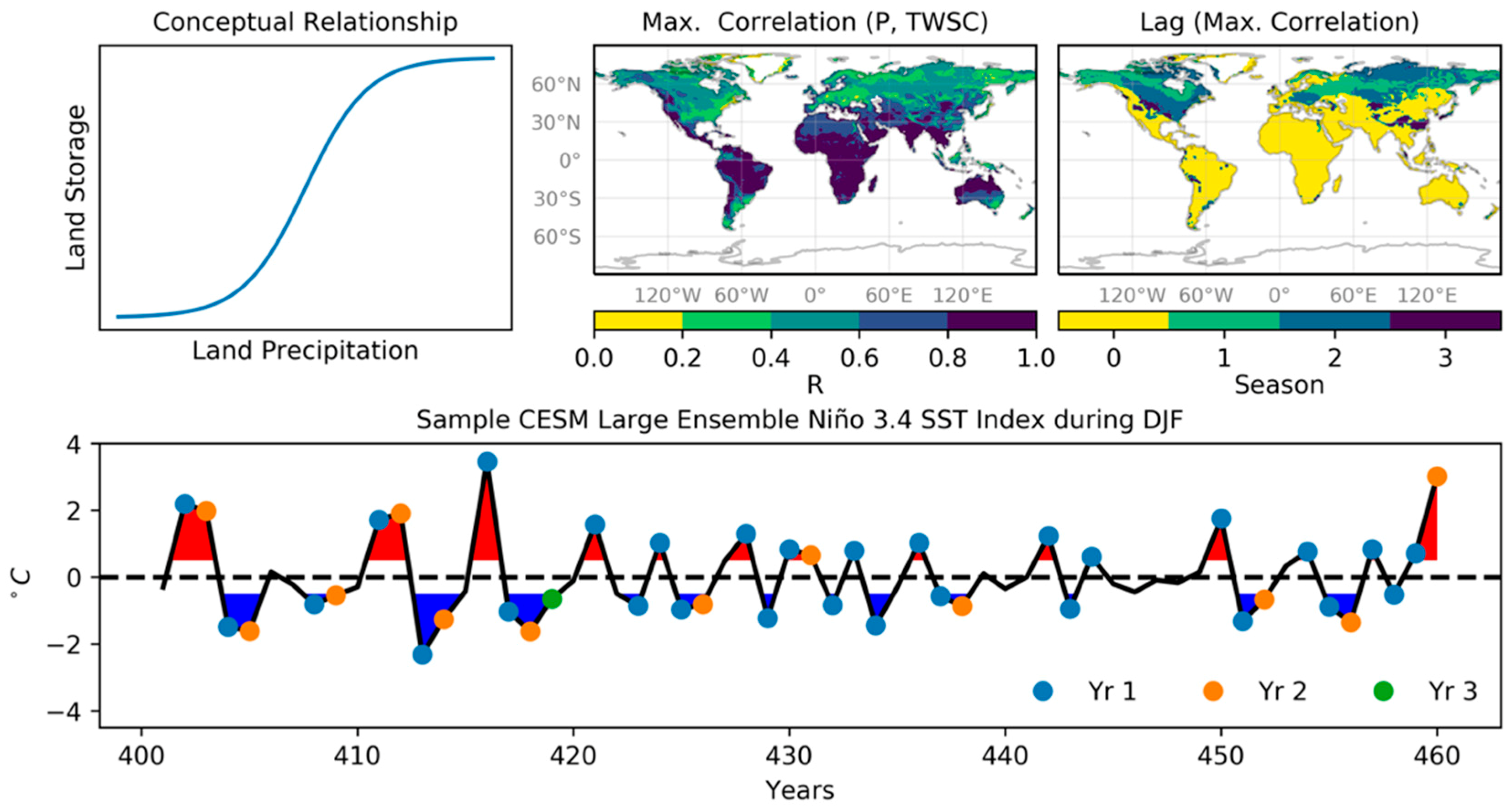
Precipitation being the main source of water over land, it is reasonable to assume that ENSO-TWS teleconnections generally follow ENSO-P teleconnections [6,24]. However, precipitation-storage relationship, while being positive, is not linear throughout. Figure 1 (top left panel) shows a conceptual relationship between precipitation and storage, often implicitly represented in rainfall-runoff or unit hydrograph curves [25]. The mid-section of the curve is linear. The upper bound corresponds to saturation-excess, where the basin is saturated and additional precipitation no longer corresponds to more storage. The lower bound corresponds to the basin drying out, where outflow rate from mechanisms such as surface and subsurface runoff and evapotranspiration fluxes exceed precipitation rates, and a further decrease in precipitation no longer corresponds to decrease in storage. All basins can be represented by this curve, but their exact range would vary depending on their mean hydrologic state. It is likely that the storage limits may be reached during anomalous perturbations due to ENSO, especially when such events extend for multiple years, such as the recent 2010–2012 La Niña. Since 1870, there have been 28 observed instances (10 El Niños and 18 La Niñas)—five of which occurred after 2000—when ENSO anomalies (based on Climate Prediction Center at National Oceanic and Atmospheric Administration http://origin.cpc.ncep.noaa.gov/) persisted into the second year. Given that anomalous storage response to ENSO is relevant to a range of stakeholders from global mean sea level researchers to water resources managers, it is important to understand the asymmetries and nonlinearities in the ENSO-TWS teleconnections. However, the lack of a long-term observational record limits investigating the TWS response to extended ENSO events. In this context, well simulated teleconnections in reliable climate models can be particularly useful.
In this paper, using a long, multi-century simulation of natural climate variability, we provide, for the first time, asymmetries in TWS response to ENSO duration and phase, as well as ENSO influence on the P-TWS relationship itself. The next section describes the model dataset and methods. In Section 3, we provide limited evaluation of simulated teleconnections against observations and characterize the spatio-temporal nature of the season-, phase-, and duration-specific asymmetries, as well as the combined influence of ENSO on the P-TWS relationship. Finally, we discuss the key results and summarize the study in Section 4.
2. Materials and Methods
Among current major global climate models, the Community Earth System Model (CESM) has been consistently found to be among the best at reproducing observed climatic mean fields and variability in several model intercomparison studies [26]. It has been noted for being one of the best models at representing ENSO asymmetry and its representation of ENSO variability has been found to be comparable to observations [27]. CESM has been widely used in projecting changes in ENSO variability in a changing climate [28,29,30,31,32,33]. Additionally, unlike several climate models, CESM’s land component Community Land Model (CLM) [34] features a 3.8 m deep soil column discretized over 10 layers, and a 42 m deep unconfined aquifer capable of storing 5000 mm of water. The scheme allows for an exchange between the aquifer and soil column, depending on the location of the water table depth. Thus, CESM is well suited to conduct teleconnection studies between land storage and ENSO. The CESM Large Ensemble (LE) project [35], which uses CESM version 1 [36], has been specifically designed to study internal climate variability and its separation from a forced response. CESM LE has been used to study linkages between water cycle changes, ENSO, and global warming [37]. Fasullo and Nerem (2016) [11] provide a rationale for applying CESM LE to global studies on terrestrial water cycle and sea level, and evaluate ENSO-P teleconnections from the model with observations. CESM LE includes a 2200-year, fully coupled control simulation that is well suited to study land storage response to multi-year ENSO events, otherwise difficult to study by observations alone.
The CESM LE control experiment (b.e11.B1850C5CN.f09_g16.005, available at http://www.cesm.ucar.edu/experiments/cesm1.1/LE/) was conducted to provide a reference for intrinsic climate variability in the absence of anthropogenic climate change. The simulation involved running a fully coupled configuration of CESM at approximately 1° horizontal resolution, and was forced with constant pre-industrial climate forcing. The forcing, which represented the radiative conditions during the year 1850, was indicative of natural climate before its anthropogenic perturbation. The climate was allowed to evolve for 2200 years. After allowing the first 400 years for model spin up, we used the remaining 1800 years for analysis.
Our choice to use the CESM LE was guided by: (1) The availability of an extended control simulation, which provided a unique way of assessing the occurrences and influences of multi-year ENSO events that observations do not permit; (2) the demonstration by previous studies of reliable representation of TWS [11]; and (3) improvement of CESM 1 over its predecessor and other climate models at representing observed ENSO power spectra and teleconnections, including their duration [32,36]. However, limitations of the model were also acknowledged including (but not limited to) its lack of an explicit human water management component (such as reservoirs, irrigation, and groundwater abstraction).
Total land precipitation and TWS are computed from other CESM LE output variables as follows [11]:
where PRECC is the convective precipitation rate for liquid and ice, and PRECL is the large-scale (stable) precipitation rate for liquid and ice, and
where SOILLIQ and SOILICE are soil liquid and ice storage, respectively, while WA, H2OSNO, H2OCAN, and VOLR are storage in aquifers, snow cover, canopy, and rivers, respectively. SOILLIQ and SOILICE were integrated across the depth of the soil column in CLM4. From TWS, the long-term mean was removed to generate TWS anomalies (TWSA). Terrestrial water storage change (TWSC), a monthly derivative of TWSA, was computed based on the terrestrial water balance equation
A local lag-correlation (at each land grid-point) between seasonally averaged TWSC and P (Figure 1, top center and right) shows that maximum correlation was achieved at zero lag over most ENSO-influenced regions [24]. Computing TWSC also accounted for observed lag between ENSO and TWS [7]. The Niño 3.4 SSTA (average sea surface temperature anomalies within Nino 3.4 region) were used to represent ENSO variability and were obtained for years 401–2200 from the Climate Variability Diagnostic Package (CVDP) [38].
The monthly time series of precipitation, TWSC, and Niño 3.4 SSTA were then seasonally averaged across December-January-February (DJF), March-April-May (MAM), June-July-August (JJA), and September-October-November (SON). They were then detrended by removal of the linear trend to focus on year-to-year variability. As demonstrated in Figure 1 (bottom), the time series were separated into non-ENSO or ‘neutral’ years when Niño 3.4 SSTA were within °C, and ENSO years when the SSTA anomalies were beyond these thresholds. The ENSO years were further separated into El Niño and La Niña years. Finally, the ENSO years were also separated based on event duration: ENSO events following a neutral year or consecutive ENSO years of opposite phases were considered Year 1 (blue markers in Figure 1 bottom). If the subsequent year was also an ENSO event of same phase, then it was indexed as Year 2 (orange markers in Figure 1 bottom). Defining ENSO events this way differed from the canonical definition of ENSO, which typically considers only DJF anomalies, and enabled inclusion of events peaking in other seasons. Instances of ENSO persisting into Year 3 or more are relatively uncommon, and hence were ignored. Following this method, in all 3775 events (749 Year 1 and 356 Year 2 events in DJF, 627 Year 1 and 262 Year 2 events in MAM, 568 Year 1 and 182 Year 2 events in JJA, and 740 Year 1 and 291 Year 2 events in SON) were extracted from the CESM Large Ensemble experiment between Years 401 and 2200.
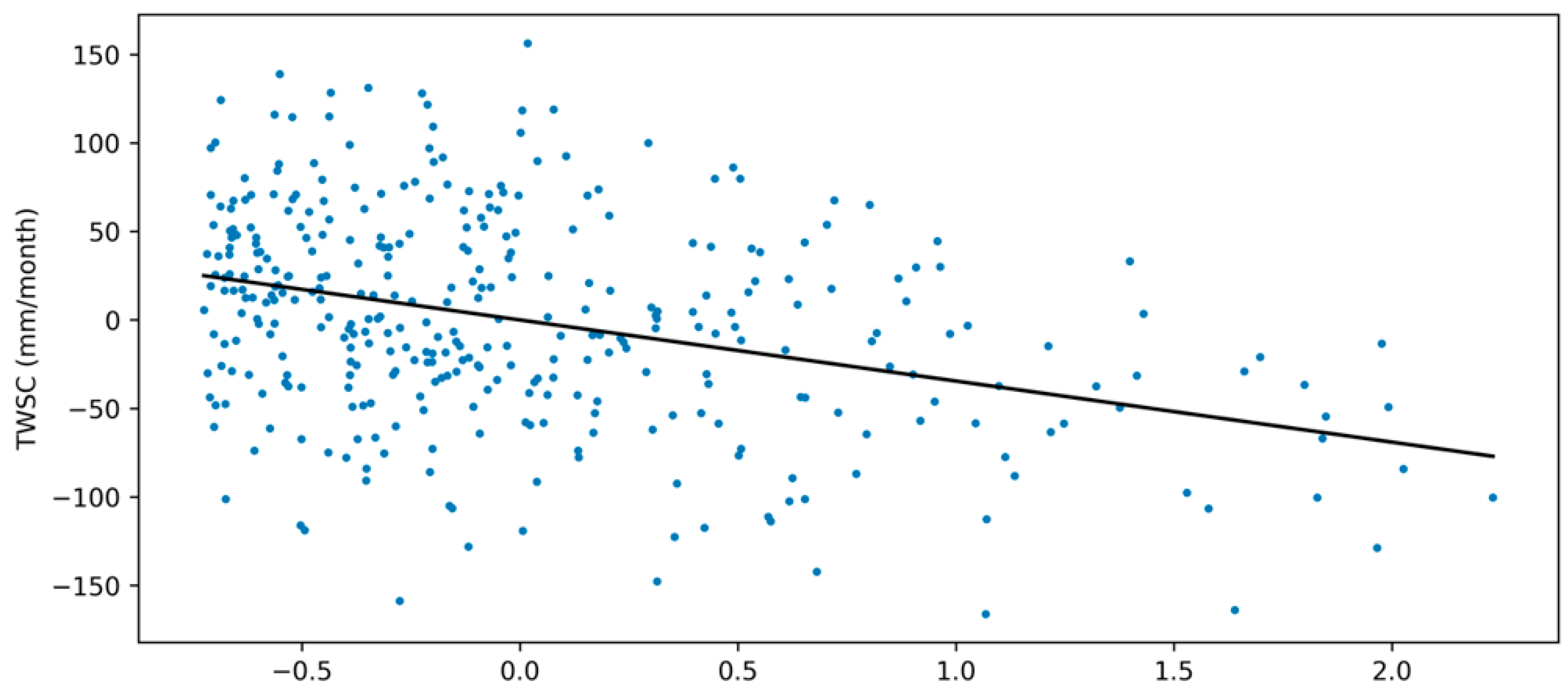
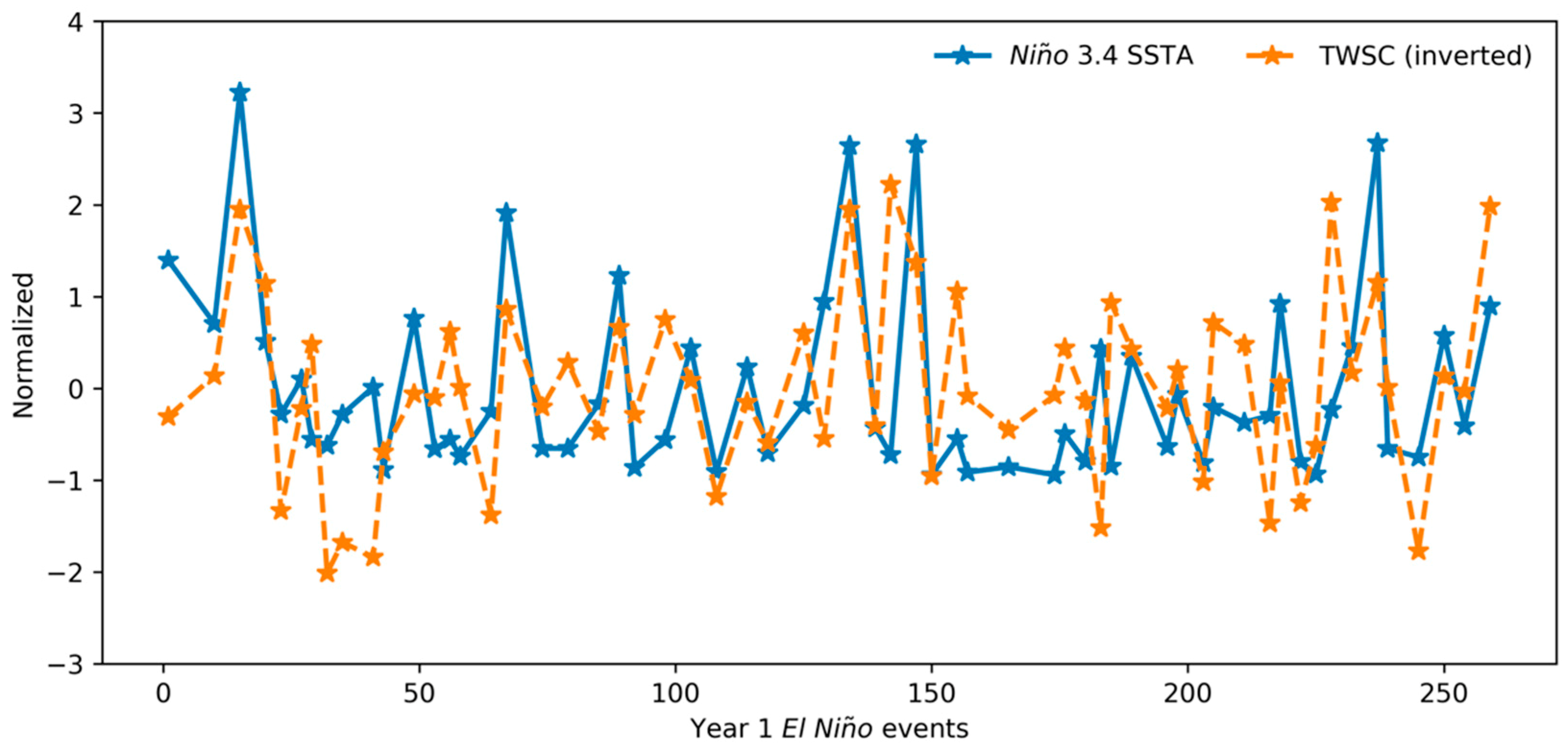
In this study, teleconnections were denoted by the slope coefficients of ordinary least squares regression (, where x and y were independent and dependent variables, and a0 and a1 were intercept and slope of their linear equation. Seasonal anomalies in Niño 3.4 SSTA were then regressed against those in TWSC at each land grid-point to provide teleconnections as . Figure 2 provides an example of regression teleconnections computed between Niño 3.4 SSTA and TWSC for Year 1 El Niños over a single location (3.3° S, 58.75° W) in the Amazon. The average teleconnection for Year 1 El Niño events for the example location was −34.5 mm/month/K (K being the abbreviation for Kelvin). Significance in the local regression coefficients were tested with a Student T-test at 90% confidence interval. Since testing regression significance at each land grid could result in rejection of the null hypothesis just by chance [39], the analyses were corrected for a false discovery rate (FDR) associated with multiple significance testing following Benjamini and Hochberg (1995) [40].
In this study, we denoted asymmetries in teleconnections as statistically significant differences in the regression coefficients. Asymmetries occurring when differencing regression coefficients between the two ENSO phases (during a given season and ENSO year) were considered as phase-specific asymmetries. Similarly, asymmetries occurring between ENSO Year 1 and Year 2 (for a given season and ENSO phase), were considered duration-specific asymmetries. Statistically significant differences in the regression coefficients were computed using a permutation test. A permutation test [41,42] is a widely used statistical technique in genomics that is particularly suited for our purpose of computing regression slope differences, since it provides a sampling distribution and accounts for size differences between the sample data points. As a walk-through for the permutation test, consider computing phase-specific asymmetries in the Niño 3.4 SSTA-TWSC teleconnections during DJF Year 1 El Niño and DJF Year 1 La Niña events. First, DJF TWSC datasets Year 1 El Niño and Year 1 La Niña events were appended together into a single dataset. Similarly, Niño 3.4 SSTA data corresponding to DJF Year 1 El Niño and DJF Year 1 La Niña were joined together into a single dataset. Random samples equaling the length of the original datasets were drawn from these joined datasets, and regression coefficients and their differences were computed. The resampling process was repeated 1000 times, providing a distribution of (n = 1000) regression slope differences. The distribution was then corrected for FDR and differences significant at 90% confidence interval were considered as asymmetries.
When describing P-TWS relationships, we fit quadratic curves (in addition to linear curves) to the P-TWSC scatter using least squares method to quantify nonlinearity in the scatter. To remove outliers, the scatter points were subjected to two-dimensional kernel density estimation (KDE) [43], a nonparametric method of computing a probability density function between two variables. Points with density less than the 10th percentile of KDE were ignored as outliers.
3. Results
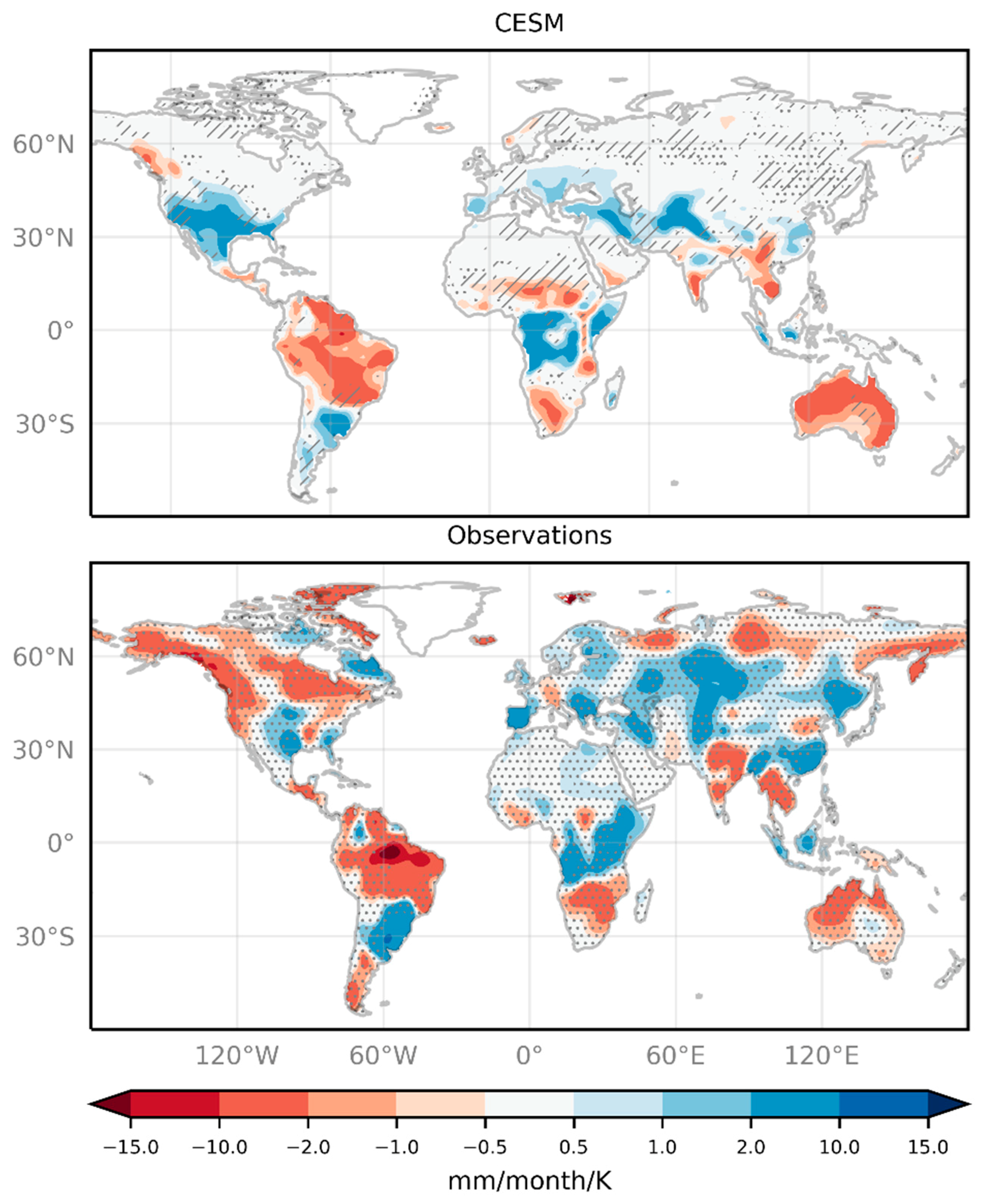
A thorough comparison of the CESM LE control run with observations of several variables, including SST and global precipitation, as well as several climate variability modes including ENSO were provided by CVDP at http://webext.cgd.ucar.edu/Multi-Case/CVDP_ex/CESM1-LENS-Controls/. While detailed model evaluation was beyond the scope of this study, we provided a limited evaluation of the simulated ENSO-TWSC teleconnections with observed teleconnections between TWS from GRACE Jet Propulsion Laboratory Mascon solution [44] and Niño 3.4 SSTA index based on Met Office Hadley Centre sea ice and SST data set (HadISST1) [45]. In Figure 3, the spatial patterns and the amplitude of the annual SSTA-TWSC regression coefficients simulated by CESM LE and those observed using GRACE and Nino 3.4 SSTA compare reasonably well despite the short observation record (15 years). Australia, South America, southern North America, southern Africa, and South, Southeast, and Central Asia show excellent agreement between model and observations. These results were consistent with Fasullo and Nerem (2016) [11] who provided further detailed evaluation of the simulated teleconnections in CESM LE between the ENSO mode and land hydrology against observations. Among regions of poor agreement (regions where teleconnection sign differs between model and observations) were the northern higher latitudes including Russia and parts of northern and central Africa. However, most of these regions also corresponded with insignificant regression coefficients in the model (overlapping hatches and stipples). We removed these regions from the analysis, and focused on well-simulated relationships.
Regression coefficients between Niño 3.4 SSTA and TWSC are analyzed separately for each season and ENSO phase during ENSO Year 1 (Figure 4) and Year 2 (Figure 5). While the broader spatial pattern seen in the annual teleconnections (Figure 3 (top)) is retained in Figure 4 and Figure 5, the differences due to season, phase, and duration are apparent. Significant teleconnections that are absent in Figure 3, likely due to averaging out the asymmetries, are seen in several regions such as eastern and northwestern North America, Central America, China, and Papua New Guinea. Several regions showed an opposing sign of regression coefficients across seasons such as Brazil during MAM, South and Southeast Asia, and South Africa in Figure 4.
Phase-specific asymmetries (shown by stippling) were widespread in Year 1, and covered an area ranging between 84 and 93 million km2, with the largest area (80% of total land area analyzed) in DJF and JJA. Year 2 phase-specific asymmetries covered a slightly smaller area on an average (74% of total land area), and the inter-season spread among the area covered also reduced. In Figure 4, the teleconnection sign reversal is seen in South and Southeast Asia and Central America during JJA and DJF, central South America during JJA, Indonesia during JJA and SON, and Australia during non-DJF seasons. Duration-specific asymmetries (shown by hatching) occurred over a relatively smaller area (averaging to 28% of total land area) compared to phase-specific asymmetries. They were most widespread during DJF and SON El Niños, followed by MAM and JJA El Niño. During La Niña, the asymmetries were most widespread during JJA and covered about 1.75 times more area than during other seasons. Dominant asymmetries occurred over Argentina and South Africa in DJF, southern Brazil over MAM and JJA, and Australia. The land areas covered by these asymmetries are summarized in Table 1.
Since ENSO influences TWSC primarily through precipitation, the asymmetries highlighted in Figure 4 and Figure 5 could also be due to asymmetries in ENSO-P teleconnections. Examining the P-TWSC relationship as a function of ENSO phase enables understanding of the ENSO influence of land storage relative to precipitation. At the same time, it provides insight into ENSO’s influence on the fundamental P-TWSC relationship (Figure 1, top left). Hence, we investigated P-TWSC relationships over two key land regions known to be influenced by ENSO: Australia and South East (SE) Asia comprised of Thailand, Cambodia, Vietnam, and Laos. We fit a quadratic curve (denoted in the figure as ‘a’) to the P-TWSC scatter as a metric of nonlinearity. We found significant departures from linearity over Australia during SON (Figure 6, top) as compared to the rest of the seasons (not shown). The quadratic coefficient increased progressively from 0.0015 month/mm during neutral years to 0.003 month/mm during ENSO Year 1 to 0.0051 month/mm during Year 2. Similarly, over SE Asia during SON (Figure 6, bottom), the P-TWSC relationship became increasingly nonlinear during ENSO Year 1 (a = −0.0015 month/mm) and Year 2 (a = −0.0028 month/mm). The likely physical mechanisms behind these nonlinearities are discussed in the next section.
4. Discussion
In this study, asymmetries in the ENSO-TWSC teleconnections are characterized for the first time as a function of ENSO phase and duration. Since several of the ENSO-influenced regions were also monsoonal, breaking down the teleconnections seasonally (Figure 4 and Figure 5) highlights the seasonal dependence of the asymmetries that were otherwise averaged out during annual averaging (Figure 3). Phase-specific asymmetries occurred over predominantly tropical and subtropical monsoon regions known to be influenced by ENSO, such as S and SE Asia, South America, southwest North America, Central America, southern Africa, and Australia. Duration-specific asymmetries were prominent during JJA La Niñas over Australia, parts of S and SE Asia, northern South America, and southwest North America. Phase-specific asymmetries were more widespread compared to duration-specific asymmetries, covering about three times the area covered by the latter. In other words, TWSC generally showed a much more widespread differential (asymmetric) response to ENSO phases than it did to back-to-back persistent ENSO events. Compared to duration-specific asymmetries, phase-specific asymmetries (1) were more prominent in terms of magnitude, (2) covered a larger area in Year 1 of ENSO than Year 2, and (3) were spread across the year more consistently showing comparable occurrences in all seasons.
We found the combined response from the seasonal ENSO-TWSC phase- and duration-specific asymmetries to be nonlinear over several regions (with overlapping stippling and hatching in Figure 4 and Figure 5), such as Australia, S and SE Asia, and parts of South America and North America. Furthermore, we found that this combined response brought about ENSO-induced nonlinearity in the P-TWSC relationship. Consistent with the expected deviations from linearity in the P-TWSC relationship (Figure 1, top left), we found that the nonlinear response was pronounced in dry regions in the dry season (demonstrated over Australia during SON in Figure 6, top), and in wet regions in wet season (demonstrated over SE Asia during SON in Figure 6, bottom). During SON over Australia, the nonlinearity increased progressively from neutral years to ENSO Years 1 and 2. The departures from linearity were suggestive of having a physical basis: Australia is an overall arid region, with a slight nonlinearity in the P-TWSC relationship existing even during neutral years (a = 0.0015 month/mm). This average nonlinearity was likely due to low rainfall amounts evaporating quickly and having little impact on TWS. Furthermore, SON over Australia is a dry season, and the storage tendency is already well below the annual average (Figure 6 top). In other words, P-TWSC curve for Australia in SON sits on the lower half of the theoretical curve from Figure 1. The teleconnections over Australia in Figure 4 and Figure 5 strengthened during Year 2 La Niñas, while they weaken during Year 2 El Niños. These changes are well reflected in P (x axis) in the Figure 6 scatter plots: Year 2 El Niños were drier while Year 2 La Niñas were wetter. However, with the land likely drying out (storage change reaching zero), no further drying from Year 2 El Niños was observed in TWSC. This caused further separation of ENSO phases in the scatter, as TWSC continued increasing due to wetter La Niñas but it no longer decreased from drier El Niños. This growing differential response to ENSO phase drives the P-TWS relationship closer to the lower threshold in the theoretical curve from Figure 1.
Contrasting against Australia, SE Asia is a seasonally wet region, with a distinct rainy season during SON. The storage, likely not yet recovered from the pre-monsoon season, corresponds linearly to the increase in precipitation during SON during average years (neutral years, a = 0.0001 month/mm). However, due to above-average precipitation during La Niñas and below-average precipitation during El Niños, the P-TWSC relationship becomes increasingly nonlinear during ENSO Year 1 (a = −0.0015 month/mm) and Year 2 (a = −0.0028 month/mm) as it moves towards the saturation-excess limit shown in Figure 1. While the overall nonlinearity during both ENSO phases increased in Year 2, unlike Australia the separation of the scatter between phases was less distinct in the ENSO Year 1 and more so in ENSO Year 2. A likely cause of this lack of distinction between phases can be found in Figure 4 and Figure 5: Over SE Asia during SON (third row), the teleconnections over El Niños (right panel) are less homogenous and not as strong in magnitude compared to those during La Niñas (left panel). Thus, the decrease in storage during El Niños was only slight compared to the increase in storage during La Niñas. A possible explanation for this was the combined interaction of the seasonal cycle and ENSO variability on TWS, which according to Hamlington et al. (2019) [8] can cause more than 20% changes in variance over parts of SE Asia. In the present case, the dominant rainy season likely overshadowed relatively drier conditions during El Niño years and pushed the P-TWSC relationship towards saturation-excess limit. This suggests that local seasonality and mean climatic state continue to remain important governing factors of the P-TWSC relationship.
The asymmetries, and the nonlinearity that they bring about, are likely to be of interest for global mean sea level researchers. The ENSO-induced nonlinearity demonstrated in P-TWSC relationship provides insight on the limits of TWS to modulate the interannual variability in global mean sea level. With the ENSO forecasting capabilities getting better, water resource managers and planners can consider the regional and seasonal asymmetries from phase and ENSO duration to better prepare and plan for the ENSO-influenced changes in the water storage systems.
Author Contributions
Conceptualization, H.A.C. and J.T.F.; Formal analysis, H.A.C.; Methodology, H.A.C. and J.T.F.; Writing—original draft, H.A.C.; Writing—review & editing, H.A.C., J.T.F., J.T.R., R.S.N., and J.S.F.
Funding
CESM LE outputs were accessed and processed at NCAR’s supercomputing clusters through Grad/Postdoc allocation request fund (project code UCIR0016).
Acknowledgments
The research was carried out at the Jet Propulsion Laboratory, California Institute of Technology, under a contract with the National Aeronautics and Space Administration (80NM0018D0004). The datasets used in this study were acquired from following sources. Niño 3.4 SSTA Index: https://www.esrl.noaa.gov; GRACE: https://grace.jpl.nasa.gov.
Conflicts of Interest
The authors declare no conflict of interest. The funders had no role in the design of the study; in the collection, analyses, or interpretation of data; in the writing of the manuscript; or in the decision to publish the results.
References
- Reager, J.T.; Gardner, A.S.; Famiglietti, J.S.; Wiese, D.N.; Eicker, A.; Lo, M.-H. A decade of sea level rise slowed by climate-driven hydrology. Science 2016, 351, 699–704. [Google Scholar] [CrossRef] [PubMed]
- Llovel, W.; Becker, M.; Cazenave, A.; Jevrejeva, S.; Alkama, R.; Decharme, B.; Douville, H.; Ablain, M.; Beckley, B. Terrestrial waters and sea level variations on interannual time scale. Glob. Planet. Chang. 2011, 75, 76–82. [Google Scholar] [CrossRef] [Green Version]
- Cazenave, A.; Dieng, H.-B.B.; Meyssignac, B.; Von Schuckmann, K.; Decharme, B.; Berthier, E. The rate of sea-level rise. Nat. Clim. Chang. 2014, 4, 358–361. [Google Scholar] [CrossRef]
- Boening, C.; Willis, J.K.; Landerer, F.W.; Nerem, R.S.; Fasullo, J. The 2011 La Nina: So strong, the oceans fell. Geophys. Res. Lett. 2012, 39. [Google Scholar] [CrossRef]
- Fasullo, J.T.; Boening, C.; Landerer, F.W.; Nerem, R.S. Australia’s unique influence on global sea level in 2010-2011. Geophys. Res. Lett. 2013, 40, 4368–4373. [Google Scholar] [CrossRef]
- Dai, A.; Wigley, T.M.L. Global patterns of ENSO-induced precipitation. Geophys. Res. Lett. 2000, 27, 1283–1286. [Google Scholar] [CrossRef] [Green Version]
- Phillips, T.; Nerem, R.S.; Fox-Kemper, B.; Famiglietti, J.S.; Rajagopalan, B. The influence of ENSO on global terrestrial water storage using GRACE. Geophys. Res. Lett. 2012, 39. [Google Scholar] [CrossRef] [Green Version]
- Hamlington, B.D.; Reager, J.T.; Chandanpurkar, H.A.; Kim, K.Y. Amplitude Modulation of Seasonal Variability in Terrestrial Water Storage. Geophys. Res. Lett. 2019, 46, 4404–4412. [Google Scholar] [CrossRef]
- Nerem, R.S.; Chambers, D.P.; Choe, C.; Mitchum, G.T. Estimating Mean Sea Level Change from the TOPEX and Jason Altimeter Missions. Mar. Geod. 2010, 33, 435–446. [Google Scholar] [CrossRef]
- Chen, J.L.; Wilson, C.R.; Tapley, B.D.; Yang, Z.L.; Niu, G.Y. 2005 drought event in the Amazon River basin as measured by GRACE and estimated by climate models. J. Geophys. Res. Solid Earth 2009, 114. [Google Scholar] [CrossRef]
- Fasullo, J.T.; Nerem, R.S. Interannual variability in global mean sea level estimated from the cesm large and last millennium ensembles. Water 2016, 8, 491. [Google Scholar] [CrossRef]
- Liang, Y.C.; Lo, M.H.; Yu, J.Y. Asymmetric responses of land hydroclimatology to two types of El Niño in the Mississippi River Basin. Geophys. Res. Lett. 2014, 41, 582–588. [Google Scholar] [CrossRef]
- Khandu, K.; Forootan, E.; Schumacher, M.; Awange, J.L.; Muller Schmied, H. Exploring the influence of precipitation extremes and human water use on total water storage (TWS) changes in the Ganges-Brahmaputra-Meghna River Basin. Water Resour. Res. 2016, 52, 2240–2258. [Google Scholar] [CrossRef] [Green Version]
- De Linage, C.; Kim, H.; Famiglietti, J.S.; Yu, J.Y. Impact of Pacific and Atlantic sea surface temperatures on interannual and decadal variations of GRACE land water storage in tropical South America. J. Geophys. Res. Atmos. 2013, 118, 10811–10829. [Google Scholar] [CrossRef]
- Eicker, A.; Forootan, E.; Springer, A.; Longuevergne, L.; Kusche, J. Does GRACE see the terrestrial water cycle “intensifying”? J. Geophys. Res. 2016, 121, 733–745. [Google Scholar] [CrossRef]
- Kusche, J.; Eicker, A.; Forootan, E.; Springer, A.; Longuevergne, L. Mapping probabilities of extreme continental water storage changes from space gravimetry. Geophys. Res. Lett. 2016, 43, 8026–8034. [Google Scholar] [CrossRef] [Green Version]
- Ni, S.; Chen, J.; Wilson, C.R.; Li, J.; Hu, X.; Fu, R. Global Terrestrial Water Storage Changes and Connections to ENSO Events. Surv. Geophys. 2018, 39, 1–22. [Google Scholar] [CrossRef]
- Yeh, S.-W.; Cai, W.; Min, S.-K.; McPhaden, M.J.; Dommenget, D.; Dewitte, B.; Collins, M.; Ashok, K.; An, S.-I.; Yim, B.-Y.; et al. ENSO atmospheric teleconnections and their response to greenhouse gas forcing. Rev. Geophys. 2018, 56, 185–206. [Google Scholar] [CrossRef]
- Okumura, Y.M.; Ohba, M.; Deser, C.; Ueda, H. A proposed mechanism for the asymmetric duration of El Niño and La Niña. J. Clim. 2011. [Google Scholar] [CrossRef]
- Choi, K.Y.; Vecchi, G.A.; Wittenberg, A.T. ENSO transition, duration, and amplitude asymmetries: Role of the nonlinear wind stress coupling in a conceptual model. J. Clim. 2013, 26, 9462–9476. [Google Scholar] [CrossRef]
- Kao, H.Y.; Yu, J.Y. Contrasting Eastern-Pacific and Central-Pacific types of ENSO. J. Clim. 2009. [Google Scholar] [CrossRef]
- Wang, S.; Huang, J.; He, Y.; Guan, Y. Combined effects of the Pacific decadal oscillation and El Nino-southern oscillation on global land dry—Wet changes. Sci. Rep. 2014, 4, 6651. [Google Scholar] [CrossRef] [PubMed]
- Hamlington, B.D.; Cheon, S.H.; Thompson, P.R.; Merrifield, M.A.; Nerem, R.S.; Leben, R.R.; Kim, K.-Y. An ongoing shift in Pacific Ocean sea level. J. Geophys. Res. Ocean. 2016, 121, 5084–5097. [Google Scholar] [CrossRef] [Green Version]
- Ropelewski, C.F.; Halpert, M.S. Global and Regional Scale Precipitation Patterns Associated with the El Niño/Southern Oscillation. Mon. Weather Rev. 1987, 115, 1606. [Google Scholar] [CrossRef]
- Dingman, S.L. Physical Hydrology; Waveland Press: Long Grove, IL, USA, 2015. [Google Scholar]
- Knutti, R.; Sedlacek, J. Robustness and uncertainties in the new CMIP5 climate model projections. Nat. Clim. Chang. 2013, 3, 369–373. [Google Scholar] [CrossRef]
- Zhang, T.; Sun, D.Z. ENSO asymmetry in CMIP5 models. J. Clim. 2014, 27, 4070–4093. [Google Scholar] [CrossRef]
- Stevenson, S.L. Significant changes to ENSO strength and impacts in the twenty-first century: Results from CMIP5. Geophys. Res. Lett. 2012. [Google Scholar] [CrossRef]
- Stevenson, S.L.; Baylor, F.K.; Jochum, M.; Neale, R.; Deser, C.; Meehl, G. Will there be a significant change to El Niño in the twenty-first century? J. Clim. 2012, 25, 2129–2145. [Google Scholar] [CrossRef]
- Vega-Westhoff, B.; Sriver, R.L. Analysis of ENSO’s response to unforced variability and anthropogenic forcing using CESM. Sci. Rep. 2017, 7, 18047. [Google Scholar] [CrossRef]
- Cai, W.; Santoso, A.; Wang, G.; Yeh, S.W.; An, S.-I.; Cobb, K.M.; Collins, M.; Guilyardi, E.; Jin, F.F.; Kug, J.S.; et al. ENSO and greenhouse warming. Nat. Clim. Chang. 2015, 5, 849–859. [Google Scholar] [CrossRef]
- Fasullo, J.T.; Otto-Bliesner, B.L.; Stevenson, S. ENSO’s Changing Influence on Temperature, Precipitation, and Wildfire in a Warming Climate. Geophys. Res. Lett. 2018, 45, 9216–9225. [Google Scholar] [CrossRef]
- Deser, C.; Phillips, A.S.; Tomas, R.A.; Okumura, Y.M.; Alexander, M.A.; Capotondi, A.; Scott, J.D.; Kwon, Y.O.; Ohba, M. ENSO and pacific decadal variability in the community climate system model version 4. J. Clim. 2012, 25, 2622–2651. [Google Scholar] [CrossRef]
- Oleson, K.W.; Lawrence, D.M.; Gordon, B.; Flanner, M.G.; Kluzek, E.; Peter, J.; Levis, S.; Swenson, S.C.; Thornton, E.; Feddema, J.; et al. Technical Description of Version 4.0 of the Community Land Model (CLM); NCAR Technical Note NCAR/TN-478+STR; National Center for Atmospheric Research: Boulder, CO, USA, 2010. [Google Scholar]
- Kay, J.E.; Deser, C.; Phillips, A.; Mai, A.; Hannay, C.; Strand, G.; Arblaster, J.M.; Bates, S.C.; Danabasoglu, G.; Edwards, J.; et al. The community earth system model (CESM) large ensemble project: A community resource for studying climate change in the presence of internal climate variability. Bull. Am. Meteorol. Soc. 2015, 96, 1333–1349. [Google Scholar] [CrossRef]
- Hurrell, J.W.; Holland, M.M.; Gent, P.R.; Ghan, S.; Kay, J.E.; Kushner, P.J.; Lamarque, J.F.; Large, W.G.; Lawrence, D.; Lindsay, K.; et al. The community earth system model: A framework for collaborative research. Bull. Am. Meteorol. Soc. 2013, 94, 1339–1360. [Google Scholar] [CrossRef]
- Yoon, J.H.; Wang, S.Y.S.; Gillies, R.R.; Kravitz, B.; Hipps, L.; Rasch, P.J. Increasing water cycle extremes in California and in relation to ENSO cycle under global warming. Nat. Commun. 2015, 6, 8657. [Google Scholar] [CrossRef] [PubMed] [Green Version]
- Phillips, A.S.; Deser, C.; Fasullo, J.T. Evaluating modes of variability in climate models. Eos 2014, 95, 49. [Google Scholar] [CrossRef]
- Wilks, D.S. “The stippling shows statistically significant grid points”: How research results are routinely overstated and overinterpreted, and what to do about it. Bull. Am. Meteorol. Soc. 2016, 97, 2263–2273. [Google Scholar] [CrossRef]
- Benjamini, Y.; Hochberg, Y. Controlling the False Discovery Rate—A Practical and Powerful Approach to Multiple Testing. J. R. Stat. Soc. Ser. B 1995, 57, 289–300. [Google Scholar] [CrossRef]
- Phipson, B.; Smyth, G.K. Permutation p-values should never be zero: Calculating exact p-values when permutations are randomly drawn. Stat. Appl. Genet. Mol. Biol. 2010, 9, 39. [Google Scholar] [CrossRef]
- Ernst, M.D. Permutation methods: A basis for exact inference. Stat. Sci. 2004, 19, 676–685. [Google Scholar] [CrossRef]
- Scott, D.W. Multivariate Density Estimation: Theory, Practice, and Visualization, 2nd ed.; John Wiley & Sons: Hoboken, NJ, USA, 2015; ISBN 9781118575574. [Google Scholar]
- Watkins, M.M.; Wiese, D.N.; Yuan, D.N.; Boening, C.; Landerer, F.W. Improved methods for observing Earth’s time variable mass distribution with GRACE using spherical cap mascons. J. Geophys. Res. B Solid Earth 2015, 120, 2648–2671. [Google Scholar] [CrossRef]
- Rayner, N.A. Global analyses of sea surface temperature, sea ice, and night marine air temperature since the late nineteenth century. J. Geophys. Res. 2003. [Google Scholar] [CrossRef]
Figure 1.
(top left) Conceptual relationship between terrestrial precipitation (P) and terrestrial water storage (TWS). (top center) Maximum lagged correlation between P and TWS change, and the corresponding lag (top right). (bottom) Example time series of Community Earth System Model (CESM) Large Ensemble (LE) Niño 3.4 SSTA (average sea surface temperature anomalies within Nino 3.4 region) during austral summer (December-January-February) for Years 410–460 from the simulation. Shaded areas categorize the years into El Niño (red) and La Niña (blue), and markers further categorize the El Niño/Southern Oscillation (ENSO) years into Year 1 (blue), Year 2 (orange), and Year 3 (green).

Figure 2.
(top) Regression scatter between Niño 3.4 SSTA and TWSC from CESM LE for Year 1 El Niño events over an example location (3.3° S, 58.75° W) in the Amazon. (bottom) Normalized time series of Niño 3.4 SSTA and inverted terrestrial water storage change (TWSC) over the example location.
Figure 2.
(top) Regression scatter between Niño 3.4 SSTA and TWSC from CESM LE for Year 1 El Niño events over an example location (3.3° S, 58.75° W) in the Amazon. (bottom) Normalized time series of Niño 3.4 SSTA and inverted terrestrial water storage change (TWSC) over the example location.


Figure 3.
Local regression coefficients between annually (June-May) averaged time series of Niño 3.4 SSTA and TWSC from CESM LE control experiment (top) and from observations from Met Office Hadley Centre sea ice and SST data set (HadISST1) and the Gravity Recovery and Climate Experiment (GRACE) (bottom). Stippling indicates locations with statistically insignificant (p-value 0.1) slope values after correcting for false discovery rate. Hatching indicates regions where the sign of regression coefficients differs between model and observations.

Figure 4.
Local regression coefficients between Niño 3.4 SSTA and TWSC during ENSO Year 1 from CESM LE control experiment, for each season and ENSO phase. Stippling indicates phase-specific asymmetries for a given year (ENSO Year 1), while hatching indicates duration-specific for a given phase (La Niña in the left, and El Niño in the right).

Figure 5.
Similar to Figure 4, but for ENSO Year 2.
Figure 5.
Similar to Figure 4, but for ENSO Year 2.

Figure 6.
Scatter between the average precipitation and TWSC from the CESM LE control experiment over Australia during the dry season (SON, top row), SE Asia during wet season (SON, bottom row). Columns indicate neutral years, ENSO Year 1, and ENSO Year 2, respectively. The marker colors indicate Niño 3.4 SSTA index anomalies. The ‘a’ indicates coefficient value of a quadratic fit (black curve). Phase-specific linear regression coefficients (slope_nino and slope_nina) are mentioned during ENSO years. Gray dashed lines indicate scatter quadrants.


Table 1.
Area under Niña 3.4 SSTA-TWSC teleconnection asymmetries based on ENSO phase and duration. Values in parenthesis indicate percentage of total land area considered in the analysis.
Table 1.
Area under Niña 3.4 SSTA-TWSC teleconnection asymmetries based on ENSO phase and duration. Values in parenthesis indicate percentage of total land area considered in the analysis.
| Asymmetry Type | Area under Asymmetry in 1 × 10⁶ km2. Values in Parenthesis Indicate % of Total Land Area. | |||
|---|---|---|---|---|
| DJF | MAM | JJA | SON | |
| Phase-specific: | ||||
| Year 1 El Niño—Year 1 La Niña | 93 (80) | 86 (74) | 93 (81) | 84 (73) |
| Year 2 El Niño—Year 2 La Niña | 88 (76) | 87 (75) | 86 (75) | 82 (71) |
| Duration-specific: | ||||
| Year 1 El Niño—Year 2 El Niño | 31 (27) | 25 (22) | 23 (20) | 31 (27) |
| Year 1 La Niña—Year 2 La Niña | 30 (26) | 30 (26) | 53 (46) | 32 (28) |
© 2019 by the authors. Licensee MDPI, Basel, Switzerland. This article is an open access article distributed under the terms and conditions of the Creative Commons Attribution (CC BY) license (http://creativecommons.org/licenses/by/4.0/).
Share and Cite
MDPI and ACS Style
Chandanpurkar, H.A.; Fasullo, J.T.; Reager, J.T.; Nerem, R.S.; Famiglietti, J.S. Asymmetric Response of Land Storage to ENSO Phase and Duration. Water 2019, 11, 2249. https://doi.org/10.3390/w11112249
AMA Style
Chandanpurkar HA, Fasullo JT, Reager JT, Nerem RS, Famiglietti JS. Asymmetric Response of Land Storage to ENSO Phase and Duration. Water. 2019; 11(11):2249. https://doi.org/10.3390/w11112249
Chicago/Turabian StyleChandanpurkar, Hrishikesh A., John T. Fasullo, John T. Reager, Robert S. Nerem, and James S. Famiglietti. 2019. "Asymmetric Response of Land Storage to ENSO Phase and Duration" Water 11, no. 11: 2249. https://doi.org/10.3390/w11112249
Note that from the first issue of 2016, this journal uses article numbers instead of page numbers. See further details here.