Numerical Modeling of Multiphase Extraction (MPE) Aiming at LNAPL Recovery in Tropical Soils


Civil Engineering Program, Federal University of Rio de Janeiro, COPPE-UFRJ, 68506, Rio de Janeiro, RJ 21945-970, Brazil
*
Author to whom correspondence should be addressed.
Water 2019, 11(11), 2248; https://doi.org/10.3390/w11112248
Submission received: 20 September 2019
/
Revised: 23 October 2019
/
Accepted: 24 October 2019
/
Published: 26 October 2019
(This article belongs to the Special Issue Subsurface Multiphase Flow and Contamination Remediation)
Abstract
:Subsurface contamination by light non-aqueous phase liquids (LNAPL) is a widespread global problem that requires appropriate techniques to remediate soil and groundwater. In this paper, the subsurface transport over multiple phases (STOMP) model was used to simulate LNAPL multiphase flow and transport during multiphase extraction (MPE) application in two Brazilian tropical soils (silty sand and oxisol) contaminated by diesel. The model was applied to a hypothetical contamination site, with the initial LNAPL thickness observed in well extraction. The first part consisted of the MPE system sensitivity analysis, varying the applied vacuum and tip tube position. The Van Genuchten α parameter and hydraulic conductivity were the properties that most affected LNAPL saturation and fluid extraction volumes. Suitable applied vacuum and tip tube position parametrization was imperative for the efficiency of LNAPL extraction. After the definition of an appropriate MPE system configuration, simulations demonstrated that the immobile LNAPL saturation affected fluid extraction and diesel oil concentrations in aqueous and gas saturation. The model applied is able to predict LNAPL contaminant behavior in porous media during MPE technique application.
1. Introduction
In the rapid urbanization that has taken place since the beginning of the last century, fossil fuels have become vitally important, and society still depends on these resources. Given the growth of their exploitation and the commercialization of their derivatives, soil and groundwater contamination is an inherent problem. The occurrence of hydrocarbon fuel leakage, which is generally lighter than water (light non-aqueous phase liquids, LNAPL), can generate widespread subsurface contamination, resulting in potentially contaminated areas that may carry major human health and environment risks.
In the case of a LNAPL leakage, its infiltration along the vadose zone occurs by the force of gravity and horizontally by capillarity. Considering factors such as the amount of LNAPL spilled and the characteristics of the porous media, part of this product can reach the water table level, where it accumulates and moves on the surface of the capillary fringe, spreading through the saturated media. Throughout infiltration into the subsoil and spreading, the compounds present in LNAPL may partition into one or more phases simultaneously, which include volatile organic compounds (gaseous phase), compounds dissolved in water (dissolved phase), and LNAPL immiscible in water that may be in a mobile (free LNAPL) or immobile (residual LNAPL) form or may also appear immobile and water-occluded (LNAPL entrapped) in the pores [1,2].
These simultaneous phases in the hydrogeological environment media generate a multiphase flow and transport, sometimes making solutions to certain issues difficult. The movement of immiscible fluids through the vadose zone and saturated zone involves various processes and is affected by many factors, which have been widely described in the literature [3,4,5,6]. For the prediction of these processes in a multiphase flow, the characteristics of the porous media, the properties of LNAPL, as well as the estimation of spilled volume and its distribution in pore spaces are essential factors for a better understanding of the contamination extent. Once the key factors mentioned above are determined, corrective actions can be implemented to reduce the concentration of contaminants. Then, the main issue is to define the most appropriate remediation technique to achieve greater efficiency and to minimize environmental risks.
One of the widely used technologies for the remediation of LNAPL-contaminated areas is multiphase extraction (MPE). The technique consists of an in situ remediation system, which performs simultaneous recovery of the contaminant constituents in its various phases (gaseous, dissolved, and free), located in the vadose zone, capillary fringe, saturated soil, and groundwater, through an applied vacuum [7]. One of the MPE technique configurations, bioslurping, uses a single conduit for the joint extraction of liquids and gases, with the main objective of the maximization of contaminant free phase extraction and the in situ enhancement of the aerobic biodegradation of aromatic hydrocarbons as a result of increased airflow [8,9]. The well has an adjustable positioning tip/slurp tube connected to a vacuum pump. It can be lowered into the desired position according to the purpose of extracting a particular fluid. Through this tube, free LNAPL can be maximally extracted along with groundwater and gas and removed from the subsurface [10,11].
Thus, the use of tools to predict the contaminants’ behavior underground may help to obtain important information, both prior to the technique implementation and during the contaminated area’s remediation [12,13,14,15,16]. This can assist in implementing better contaminated area management strategies and choosing the best remediation technique, leading to cost savings. However, before models can be the tools of choice, they must be fully predictable [17].
Over the last few years, some multiphase models have been used to simulate multiphase transport and partitioning in subsurface systems when applying the MPE technique [14,16,18,19]. These models should include the fundamental governing equations and their constitutive relations that describe the multiphase flow, transport, and mass transfer that occur throughout extraction. In addition to simultaneous fluid recovery, the application of MPE predictions also needs to include equations that describe both saturated and unsaturated media and the evaluation of dissolved or volatilized contaminants throughout the process, which the developed module addresses.
One of the models that can be used for this type of problem is presented in the subsurface transport over multiple phases (STOMP) software. The tool was created for numerical predictions regarding the subsurface flow and transport of volatile or nonvolatile organic contaminants and, consequently, allows the modeling of various remediation systems [20,21,22,23]. Souza et al. [16] developed a module for STOMP capable of simulating MPE systems, which uses the concept of the well model to simulate the simultaneous removal of the fluids present in both saturated and unsaturated media through the bioslurping configuration. In the paper, the authors used the module to perform a sensitivity analysis of a bioslurping system by varying well characteristics and operating parameters, using soil data from the literature. In addition, the authors evaluated the influence of the soil hydraulic properties’ variation on the recovery, which resulted in a high sensitivity of fluid extraction due to hydraulic parameters, especially soil hydraulic conductivity.
The present work consists of using a STOMP bioslurping module to simulate multiphase extraction under different system configurations using laboratory-measured hydraulic parameters of two natural Brazilian tropical soils and contaminant parameters. The first part consisted of the sensitivity analysis of an MPE system under hypothetical initial conditions, varying the applied vacuum and the different elevations of the bioslurping tip tube. The comparative analysis of contaminant behavior performed in each porous media and the corresponding technique’s achievements defined a suitable extraction configuration. For this extraction configuration, a second stage of simulations was accomplished to evaluate the influence of LNAPL entrapment on fluid recovery, and finally, to analyze the influence of the MPE system operation on dissolved and volatilized phases of the contaminant in the soil mass.
2. Materials and Methods
The methodological plan can be divided into two stages: (i) experimental analysis in the laboratory, involving soil characterization and hydraulic property determination as the saturated hydraulic conductivity and soil water retention curve (SWRC), as well as the selected fuel density, viscosity, surface, and interfacial tension; and (ii) numerical analysis, represented by STOMP modeling, followed by sensitivity study and data processing.
2.1. Experimental Methods
The soil physical and mineralogical properties were determined in the Geotechnical Laboratory of Graduate School and Research in Engineering of Federal University of Rio de Janeiro (COPPE/UFRJ). The granulometric analysis was performed using the sedimentation and sieve Brazilian standard analysis [24], and the bulk density was determined using the pycnometer Brazilian standard method [25]. The mineralogical analysis was performed with x-ray diffraction in a Bruker D4 Endeavour with a cobalt x-ray tube. The samples were analyzed between the 4° and 70° 2θ range. The hydraulic saturated conductivities were measured by variable and constant head methods in laboratory permeameters. The soil water retention curve (SWRC) was determined by two different methods in order to cover a broad range of water pressure heads from less than 10 cm up to 15000 cm. For the lower pressure range (h < 1000 cm H2O), a Hyprop apparatus was used, which applies the evaporation method. For the higher pressure range (1000 < h < 15000 cmH2O), the pressure plate extractor method was applied. The SWRCs were adjusted by the van Genuchten [26] model with Mualen unsaturated hydraulic conductivity function using RETC software version 6.02.
A disturbed silty sand soil sample was collected from a metropolitan region of Rio de Janeiro. In order to compare the Multiphase Extraction modeling, data of an oxisol water retention curve from Piracicaba, State of São Paulo, were also used [27]. This soil was analyzed by the same methods described above. The results obtained for both soils can be seen in Table 1.
The Brazilian S10 Diesel was the LNAPL used in the experiment. It was analyzed in the Chemistry Laboratory of Chemical Engineering Program—COPPE/UFRJ—for viscosity and density determinations [28]. Moreover, fundamental parameters for multiphase flow simulation, such as the interfacial tension between oil and water, were obtained through the Wilhelmy plate [29]. The diesel characterization parameters are presented in Table 2.
2.2. Numerical Analysis
The software STOMP bioslurping module [16,30] was used to simulate the multiphase extraction. STOMP generates numerical predictions regarding flow and transport phenomena in the subsurface, including non-isothermal conditions, fractured medias, multiphase systems, fluid trapping, and saturated and non-saturated contaminated environments [31]. Furthermore, the model includes the main processes and parameters that result in LNAPL constituents mass losses from the subsurface and, among the existing multiphase models of natural source zone depletion, STOMP is one of the feasible simulators to model the bioslurping technique [32].
STOMP quantitative results come from a partial differential equation solution for spatial discretization and temporal domains that describe the mass transport and flow in subsurface. The dependence between secondary and unknown primary variables introduces non-linear equations, which can be represented, mainly, by relative permeability–saturation–pressure (k–S–P) functions. The conservation equations were converted to an algebraic form using the finite volume approach applied to structured orthogonal grids and Euler backwards time differencing. The algebraic system expressions were solved simultaneously using the Newton–Raphson iteration technique, determining the nonlinearities [20]. For the simulations reported in this paper, the maximum number of Newton–Raphson iterations was 16, with a convergence factor of 10−6.
Relative permeability expressions () of aqueous (l), LNAPL (n), and gaseous (g) phases were presented by Parker [3] using Mualem pore distribution theory, as stated below.
where:
- m: van Genuchten hydraulic parameter (–);aqueous, NAPL, and gaseous relative permeability (–);
- aqueous, NAPL, and gaseous effective saturation (–).
We assumed that aqueous phase and total liquid saturations (subscript t) in a water-wet system were independent functions of the LNAPL–aqueous phase and gas–LNAPL capillary pressure heads, defined as, respectively,
where:
- : NAPL pressure head (m);
- : aqueous pressure head (m);
- : aqueous, NAPL, and gaseous pressure;
- reference density (generally water; kg m−3);
- gravity acceleration (m s−2).
Based on van Genuchten [26] relations, the capillary pressure and saturation functions can be scaled using the interfacial tension of given fluid pairs [3], as follows:
where:
- : effective saturation (–);
- α, m, n: van Genuchten parameters;
- h: pressure head (m).
The scaling factors and are estimated from interfacial tensions (σ):
where:
- air–water interfacial surface tension (N m−1);
- air–LNAPL interfacial tension (N m−1);
- LNAPL–water interfacial tension (N m−1).
The bioslurping module considers the well model concept in order to access flow and transport in extraction well surroundings, without using vertical equilibrium conditions in saturation calculations [16,33]. This allows three-dimensional simulations, resulting in multiphase extraction predictions, which are more comparable with real remediation cases. During simulations, STOMP calculates LNAPL saturations along x, y, and z directions through well initial pressures and constitutive relations (k–S–P) equations over time. This remediation simulation takes into account mass extracted oil, air and water. Starting from the point at which the tip tube is located, the liquid’s height above this point is determined using the local pressure and fluid densities, assuming hydrostatic conditions in the well [30].
The expression describing mass removal by bioslurping can be observed in Equation (10). The full description can be seen in Matos de Souza et al. [16]:
where:
- : mass fraction of component c (water, air, oil) recovered (Kg);
- : modified Peaceman well index (m3);
- : pressure at the bioslurping tip in phase γ (aqueous, gas and LNAPL) (Pa);
- : user-imposed well pressure converted into gauge pressure in the STOMP (Pa);
- : phase γ (aqueous, gas, and NAPL) density (Kg m−3);
- : mass fraction of component c (water, air, and oil) in phase γ (–);
- : relative permeability of fluid phase γ (–);
- : viscosity of phase γ (Pa.s).
All simulations were carried out in the STOMP bioslurping module using a two-dimensional domain, cylindrical coordinates, and a uniform and homogeneous porous media. The domain for all simulations included a hypothetical extraction well at the first node, with its surroundings extending 10 m into the radial direction (r-direction) and 12 m in the vertical direction (z-direction). Hypothetical contamination with a known distribution was also assumed, considering aquifer recharge and no additional oil spill after the simulation started. The boundary conditions were established in four directions: inner, outer, top, and bottom. The inner plane was located in the well extraction center (r = 0); thus, no fluid contribution comes from this point. Impermeable surfaces were set in the top and bottom planes, meaning there is no fluid contribution in these boundaries either. Supposing a multi well extraction field, where the influence radius of a well terminates in the influence radius of the other, without intersections, zero flux conditions for LNAPL were considered through the radial outer boundary, but water and air fluxes were allowed.
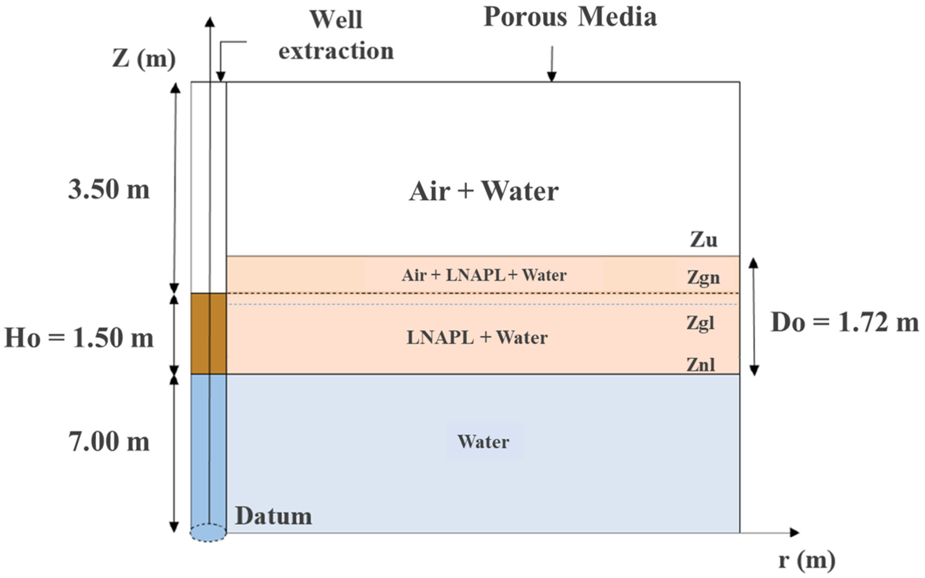
The Figure 1 represents the initial conceptual model, in which fluid interfaces, layer constituents, and the apparent vertical LNAPL thickness (H0) observed in the well extraction, as well as the real vertical oil thickness in soil (D0) can be seen. For the test problem, the NAPL thickness in the well (Ho) was 1.5 m, the bottom of the domain was z = 0 m, znl (LNAPL–aqueous phase interfaces in the well) was at z = 7.00 m, zgn (gas–LNAPL phase interfaces in the well) at z = 8.50 m, and zgl (the water table location) was at z = 8.2 m, which was obtained from equations presented in Souza [16]. The corresponding soil LNAPL thickness (Dn = distance between Zu and Znl) was 1.72 m, representing the zone where Sn > 0 was obtained according to Lenhard and Parker [34] formulation.
Taking into account all the parameters above, a well extraction of 4’ and well screening of 2 m, simulations were performed concerning the MPE system. The total extraction simulation time was 100 days for all simulations.
The first set of test simulations was performed to determine the fluid production characteristics as a function of the vacuum applied (VA) and tip tube position (TE) in the well. For these tests, we considered nine different vacuum pressures (VA1 = 0.00, VA2 = 1.33, VA3 = 2.66, VA4 = 6.00, VA5 = 11.33, VA6 = 12.40, VA7 = 24.93, VA8 = 49.86, and VA9 = 66.26 kPa) and all possible combinations with nine tip tube positions z (TE1 = 6.85, TE2 = 7.05, TE3 = 7.25, TE4 = 7.55, TE5 = 7.75, TE6 = 7.95, and TE7 = 8.25 m) located in water (TE1), the oil–water interface (TE2), oil (TE3, TE4, TE5, TE6, and TE7), air–oil interface (TE8), and air (TE9). In addition, the results obtained with these combinations were discussed operationally, taking into account the hydraulic properties of soils.
From the results analysis, a suction tip tube position and vacuum pressure pair, which presented an adequate yield in both soils was defined for the following steps. In the first stages in which the applied vacuum and the tip tube positioning were evaluated, factors including the residual and trapped LNAPL were disregarded. After defining a suitable configuration, the effective maximum entrapped and residual LNAPL saturation formed by the water movement resulting from the vacuum application were added to the simulations. These factors were included for the further analysis of fluid extraction and also the evaluation of the dissolved and volatilized oil phases by the remediation system. The longitudinal and transversal dispersivities of oil were considered to be 0.056 m and 0.0056 m, respectively, and the retardation coefficient was disregarded.
3. Results
3.1. Soil Water Retention Curve (SWRC)
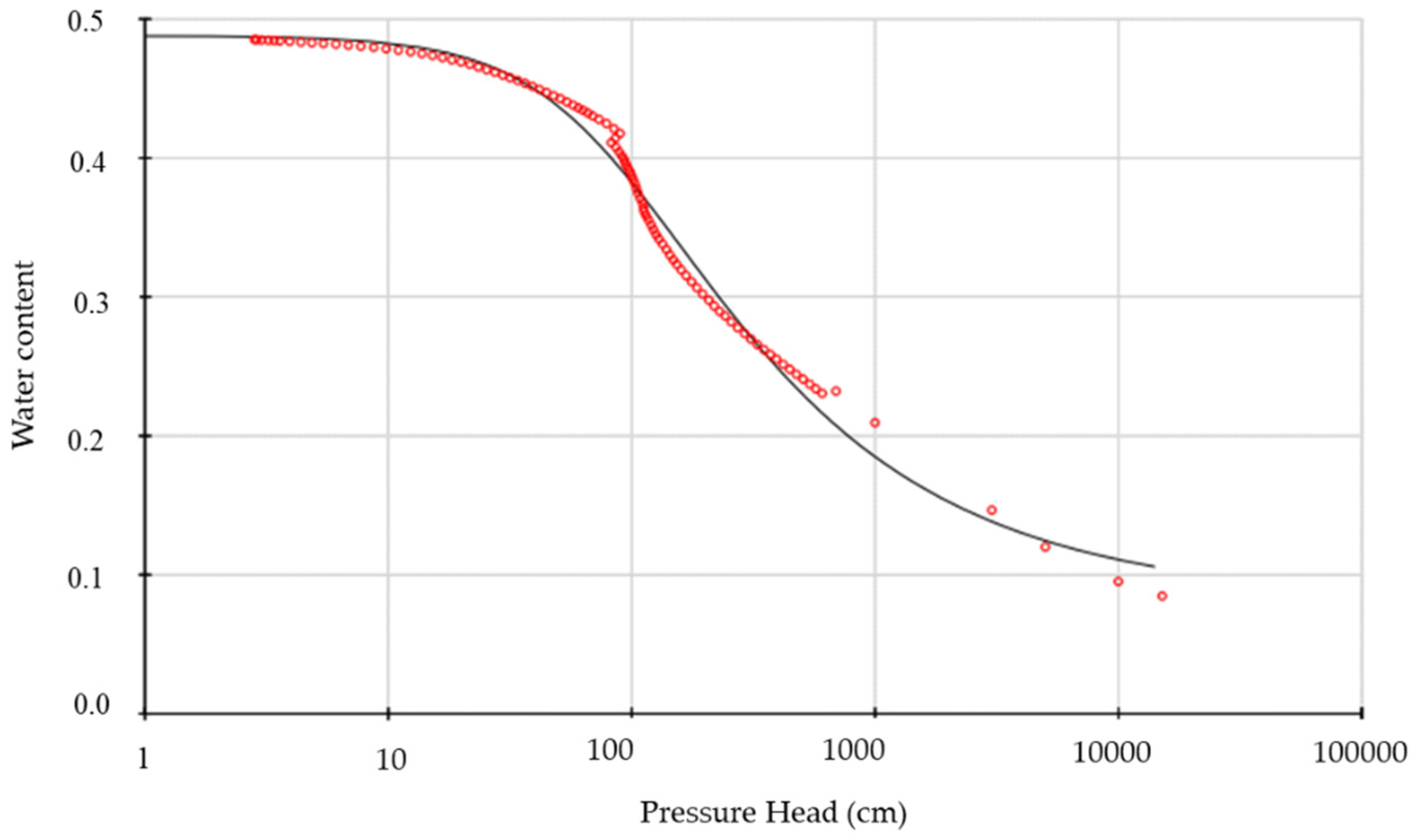
Figure 2 shows the SWRC obtained from silty sand soil after fitting data into a unimodal pore-size distribution. For comparison, the oxisol SWRC is presented in Figure 3.
Despite the lower amount of small grains in silty sand soil compared to the oxisol, its hydraulic conductivity is lower. In addition, the SWRC values differ greatly from each other. The silty sand SWRC presented a smoothed reduction in water saturation as the pressure head increased, suggesting a porous media with a better graduated pore size distribution.
On the other hand, in the oxisol SWRC, a sharp drop of water saturation can be seen at low pressure heads, which is typical of granular soils. Due to intense weathering and leaching, the oxisol fine particles tend to rearrange into aggregates [35], resulting in a discontinuous and highly heterogeneous granular particle structure. This strongly modifies the soil pore size distribution, that, along with mineralogy and clay content, directly influences the saturated hydraulic conductivity and hydraulic behavior. Ferreira et al. [36] observe that it is reasonable to assume that, in oxisols, the saturated hydraulic conductivity (Ks) may increase with the fine particle content, showing that the physical properties associated with the soil structure are markedly influenced by the mineralogy of the clay fraction [37]. In the oxisol x-ray analysis, the presence of kaolinite, hematite and gibbsite was detected, which are aluminum and iron oxide minerals that contribute to the soil particle agglomeration.
This behavior was not observed in the silty sand soil. Although presenting fewer fine particles than the oxisol, these fine particles are arranged as independent elements, resulting in smaller and better distributed pore sizes. These features increase the fluid infiltration and extraction resistance, smoothing the SWRC form. The silty sand mineralogical analysis indicated that quartz was clearly dominant, with the presence of aluminum silicates (kaolinite, muscovite, microcline, and diopside).
For this reason, even if the particle size composition of the two soils is not as varied, the van Genuchten parameters and the saturated hydraulic conductivity differ substantially among the soils. The van Genuchten [26] retention parameter α is considered to be an approximation of the gas entry inverse pressure in the soil, varying from clay (low α values) to sand (high α values). The parameter n is a factor indicating pore uniformity. Due to the aggregation of oxisol clay particles, it presented α parameter twice bigger than silty sand (1.31 m−1 to silty sand and 2.77 m−1 to oxisol).
The main input parameters for numerical models of transient water flow and contaminant transport in the unsaturated zone need to be in agreement with the porous media to be modeled. These differences in soil parameters influence LNAPL behavior and its recoverability by the bioslurping multiphase extraction technique, as will be seen later on.
3.2. Vacuum Applied and Slurped Volume
Before multiphase extraction had started (t = 0), the initial diesel saturation varied between 0.00 to 0.37 for the oxisol and from 0.00 to 0.09 for the silty sand soil. Meanwhile, the mass in domain was 38,092 kg and 12,480 kg for oxisol and silty sand respectively. In the code proposed in STOMP, the oil saturation in the domain was calculated from the model developed by Lenhard and Parker [34], which evaluated the soil LNAPL behavior from an oil thickness in the extraction well. This behavior indicates that the same oil thickness observed in a well extraction will present different oil quantities and distribution depending on the soil characteristics. Estimating LNAPL volumes in porous media from thicknesses detected in wells without accounting for soil properties and fluid characteristics may yield information that is inconsistent with reality.
Lenhard et al. [38] point out that the difference in pore size distributions is the main factor affecting the difference in the predicted LNAPL volume, which is also verified among the tested soils. Matos de Souza et al. [16] show that the greater the α values, the greater the initial NAPL saturations in soils. As a result, oxisol is capable of retaining more LNAPL than silty sand under prominent capillary pressures. Moreover, it should be noted that, under the same contamination conditions, the formation times of the same LNAPL thicknesses would also be different.
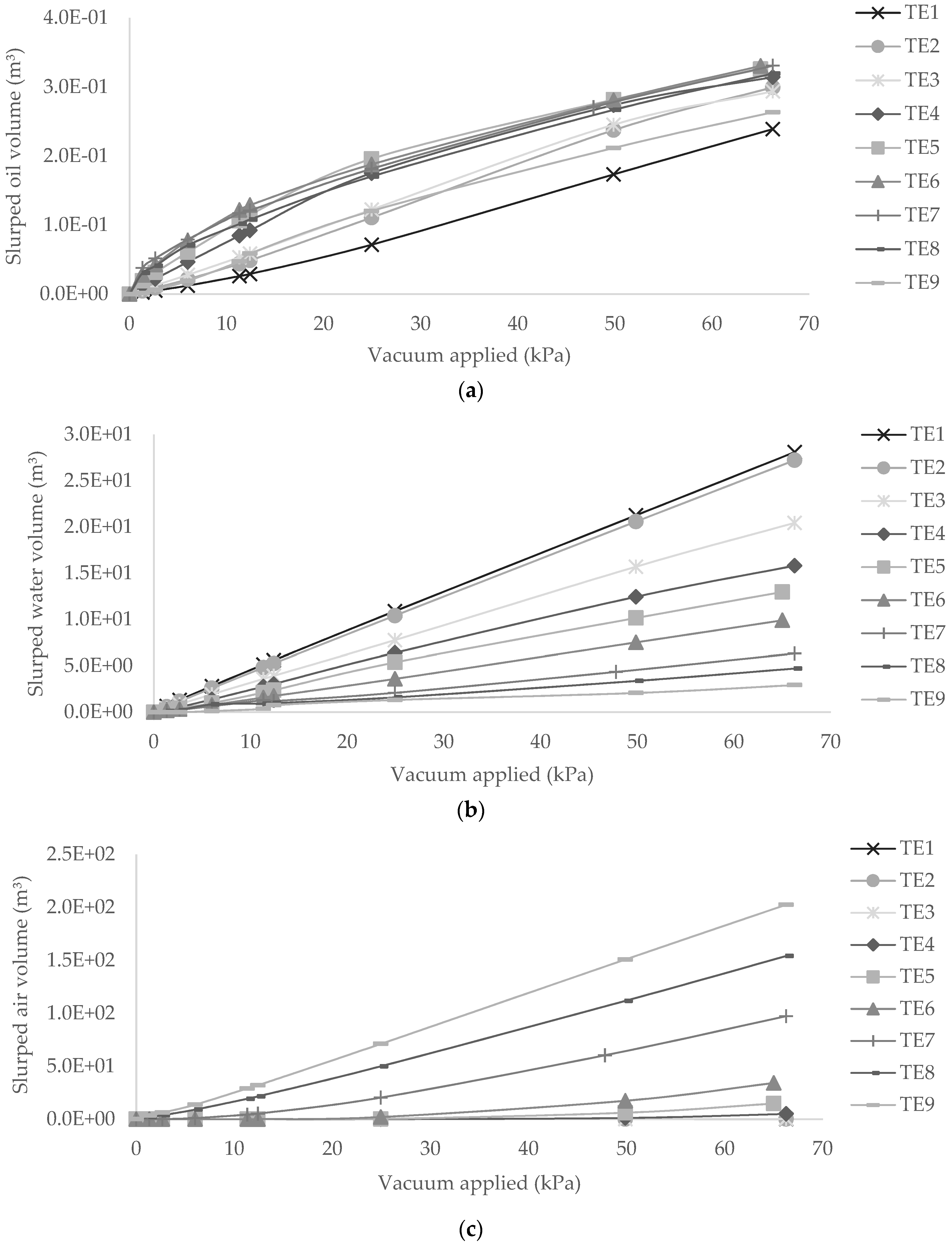
Figure 4 shows the amount of slurped oil, water, and air after 100 days as a function of vacuum pressure and tip tube position in the silty sand soil. Overall, the relationship between the applied vacuum and volume of fluids extracted was directly proportional; in other words, the greater the vacuum pressure, the greater the volume of fluids recovered in this soil. Over 100 days, the volume of oil recovered reached its maximum (0.3 m3) at 66.26 kPa, whilst under the same conditions, 3 m3 and 250 m3 of water and air were extracted.
As a MPE system operating in a bioslurping configuration has the main aim of free oil phase optimization, a suitable vacuum would be one capable of extracting the maximum of oil without extracting too much air or water. Moreover, the application of strong vacuums involves increasing operation expenses and more complex fluid treatment systems. At the same time, the selected vacuum needs to overcome the capillary forces in soil, allowing the oil flow towards the well, and it cannot reach such a great value; otherwise, it may break the interconnected LNAPL-filled pores, resulting in trapped zones that will make remediation difficult [8].
Concerning the tip tube parameter, the amount of slurped fluid is strongly dependent on its position. As expected, if the tip tube is located inside a given fluid, the slurped volume of this specific fluid will be greater compared to the other positions, as observed by Matos de Sousa [30].
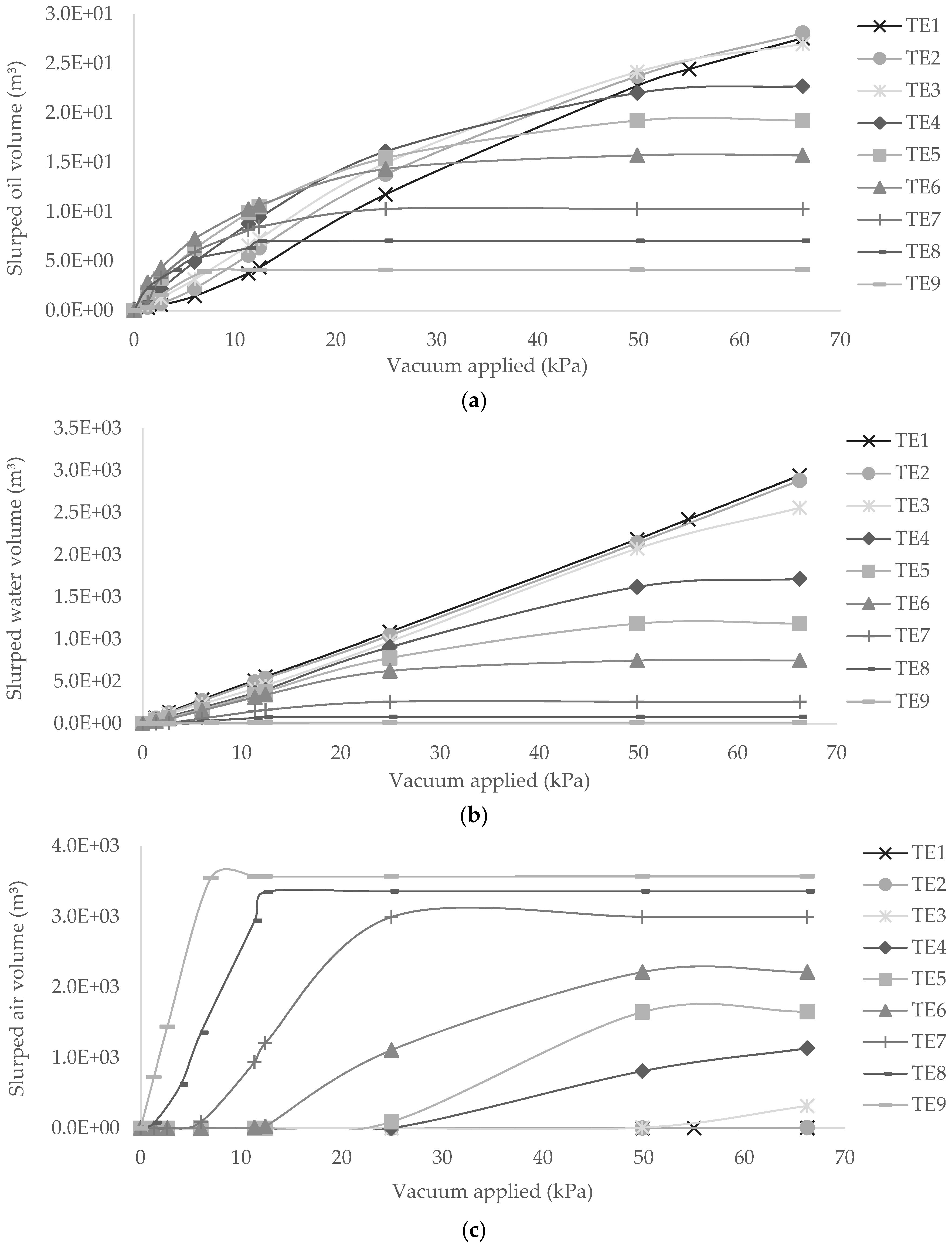
Figure 5 shows the amount of slurped oil, water, and air after 100 days as a function of vacuum pressure and tip tube position in the oxisol.
The oxisol results presented corroborate the previous statements regarding the dependence of the applied vacuum and the tip tube positioning on the slurped volume. However, in the oxisol, all fluids exhibited a maximum extraction point at which increasing the applied vacuum did not improve the volume recovery. In fact, for each positioning and fluid, there was a vacuum for which the extraction volume becomes constant. Although this pattern was not observed in the silty sand soil, this did not mean that a similar behavior would not be expected if higher vacuums were applied. As can be seen in Figure 5a,b, some tip tube positions did not reach the constant point mentioned, even under the strongest vacuum tested. However, overly increasing the applied vacuum could result in an economically unfeasible MPE system.
Besides, it can be also noticed in Figure 5c that, for air, the closer the tip tube location to this fluid, the faster it will reach the slurped stationary value, suggesting that contamination recovery by volatilization did not require strong vacuums in the oxisol.
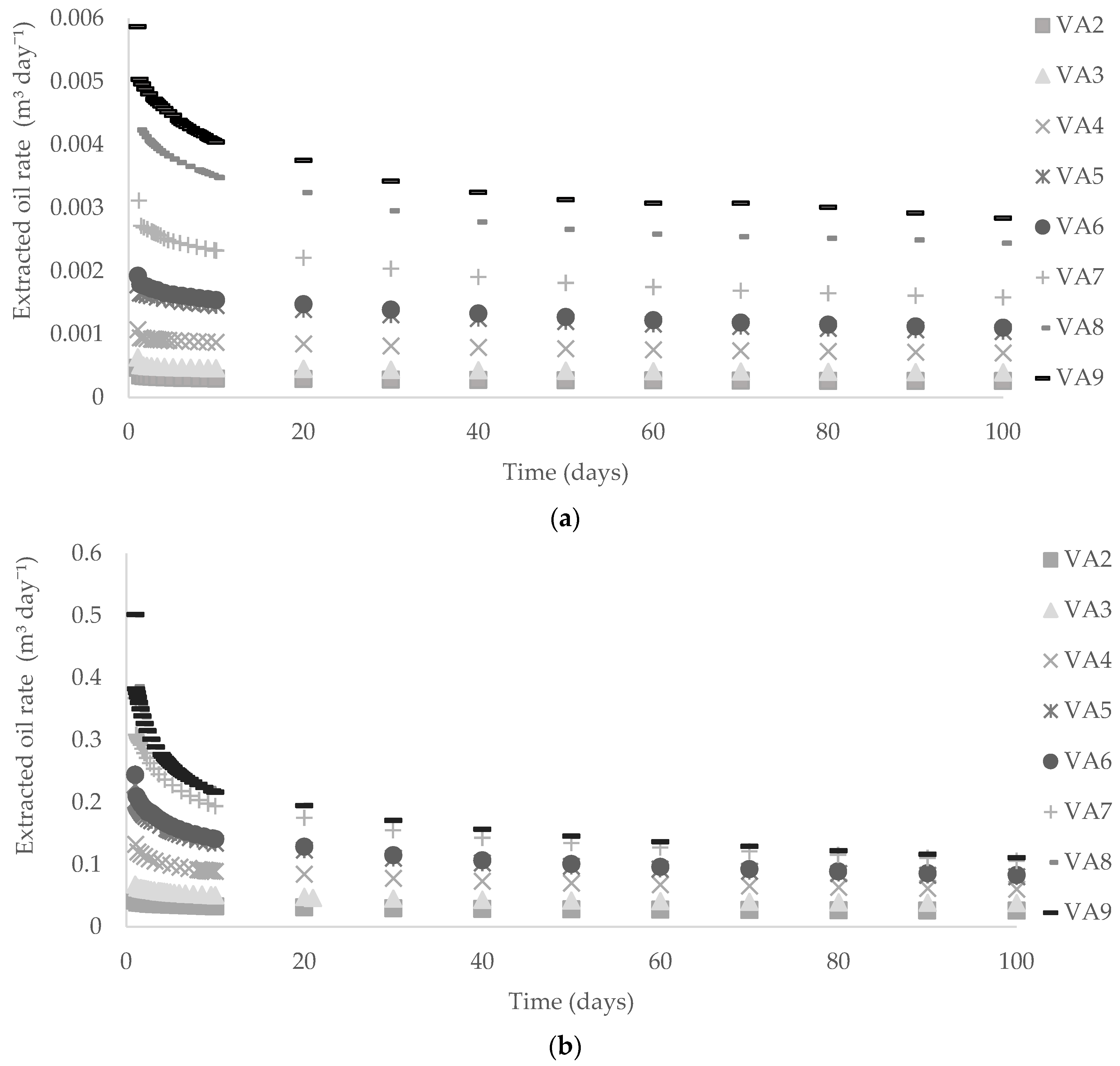
Regarding fixing a tip tube position in order to evaluate the influence of a vacuum on fluid extraction and its behavior over time, Figure 6 shows the free LNAPL extraction rates obtained from the MPE system simulations operating continuously for 100 days at the TE6 position (at z = 7.95 m) on silty sand (a) and on oxisol (b). The tip tube positioning was defined based on its performance in fluid removal, but the discussion about positioning will be presented later.
It is observed that, with vacuum application, the extraction rates started with high LNAPL recovery rates, especially with larger vacuums, but these rates decreased over time, reducing the oil recovery efficiency. The same was observed by Kacem and Benadda [39], who developed an MPE model and found that, in their hypothetical simulation, under different conditions, the toluene extraction rate in the first 14 days was 0.18 m3 day−1, decreasing significantly throughout the extraction period.
The bioslurping configuration seeks to improve the recovery of free products without extracting large amounts of groundwater [10]. Therefore, this behavior means that a 100-day intermittent system might not be the best way to use an MPE system. Periodic vacuum tip tube position adjustments to track groundwater changes and LNAPL layer thickness, or varying the vacuum applied over time, might be some procedures to maximize oil recovery.
In addition, it can be seen that water and air extraction rates tended to start with low values but might intensify over time. It was also found that under conditions of strong extraction well vacuums (VA8 and VA9) in both soils, water, and especially air volumes tended to increase almost exponentially over time. As an example, it was observed that, applying a vacuum of 24.93 kPa at TE6, the rate of air extraction over 100 days ranged from 0.003 to 0.026 m3 dia−1 in silty sand and from 3 to 13 m3 dia−1 for oxisol, while an applied vacuum of 66.26 kPa in TE6 results in extraction rates ranging from 0.07 to 0.47 m3 day−1 for silty sand and between 18 and 22 m3 day−1 for oxisol. Therefore, the application of excessively strong vacuums in a porous media, in addition to the complications in the treatment and the possibility of causing oil discontinuities in the porous media, does not necessarily provide significant gains regarding the recovery of the soil mobile oil phase [8,30].
The vacuum applied to a bioslurping well should be sufficiently high to overcome the capillary forces of the surrounding soil, stimulating LNAPL flow towards the well. Therefore, it can be seen that the magnitudes of the fluid volumes extracted between the two soils were quite different, due to the soil conditions and consequent volume. As expected, the increase in applied vacuum values also led to an increase in the volume of fluid extracted. However, this increase might not necessarily be advantageous as it might bring higher costs and the need for more elaborate effluent treatment systems and might have potential consequences on LNAPL behavior in the environment, such as the increase in trapped LNAPL, increasing persistent contamination.
3.3. Aqueous and Total Liquid Saturation
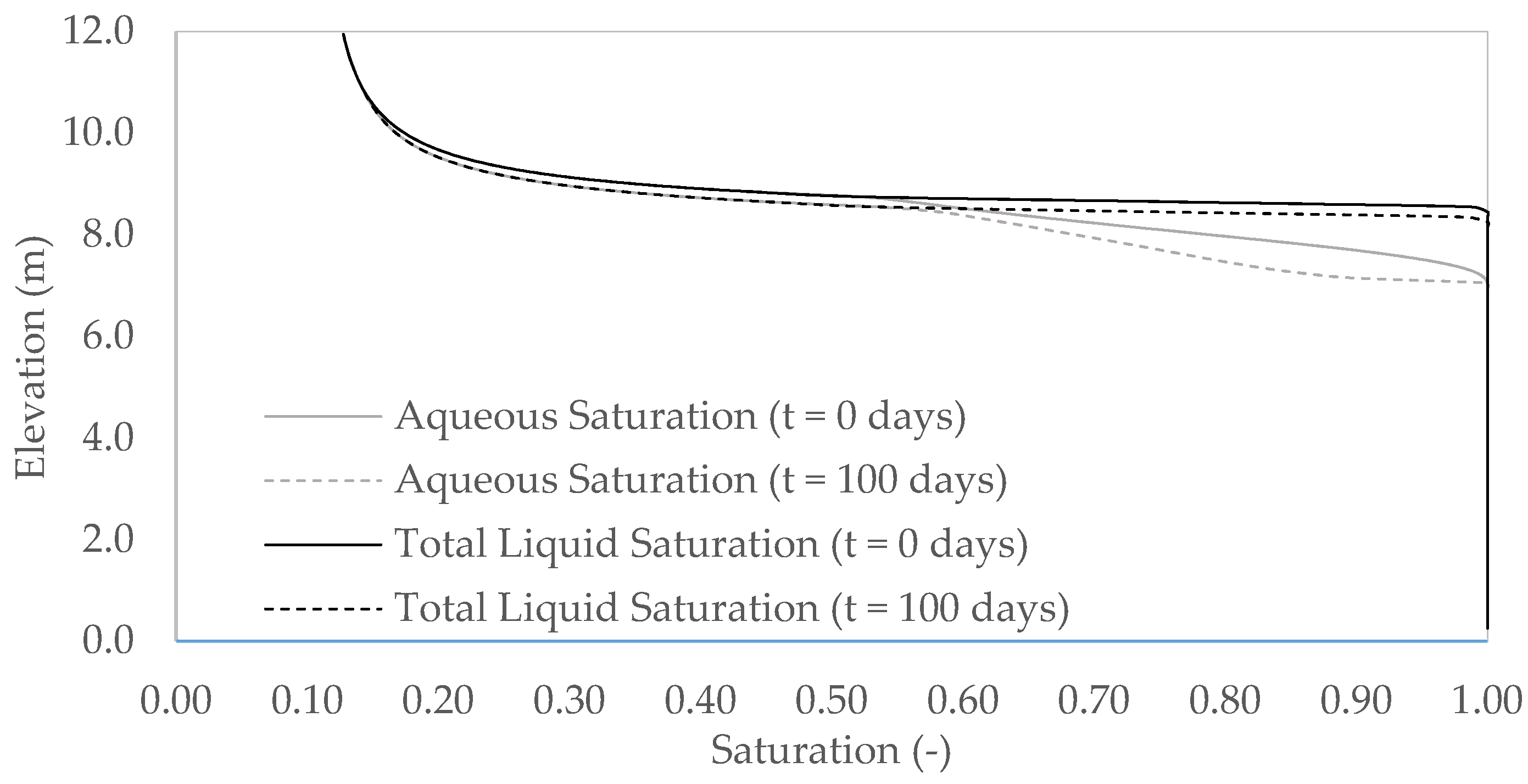
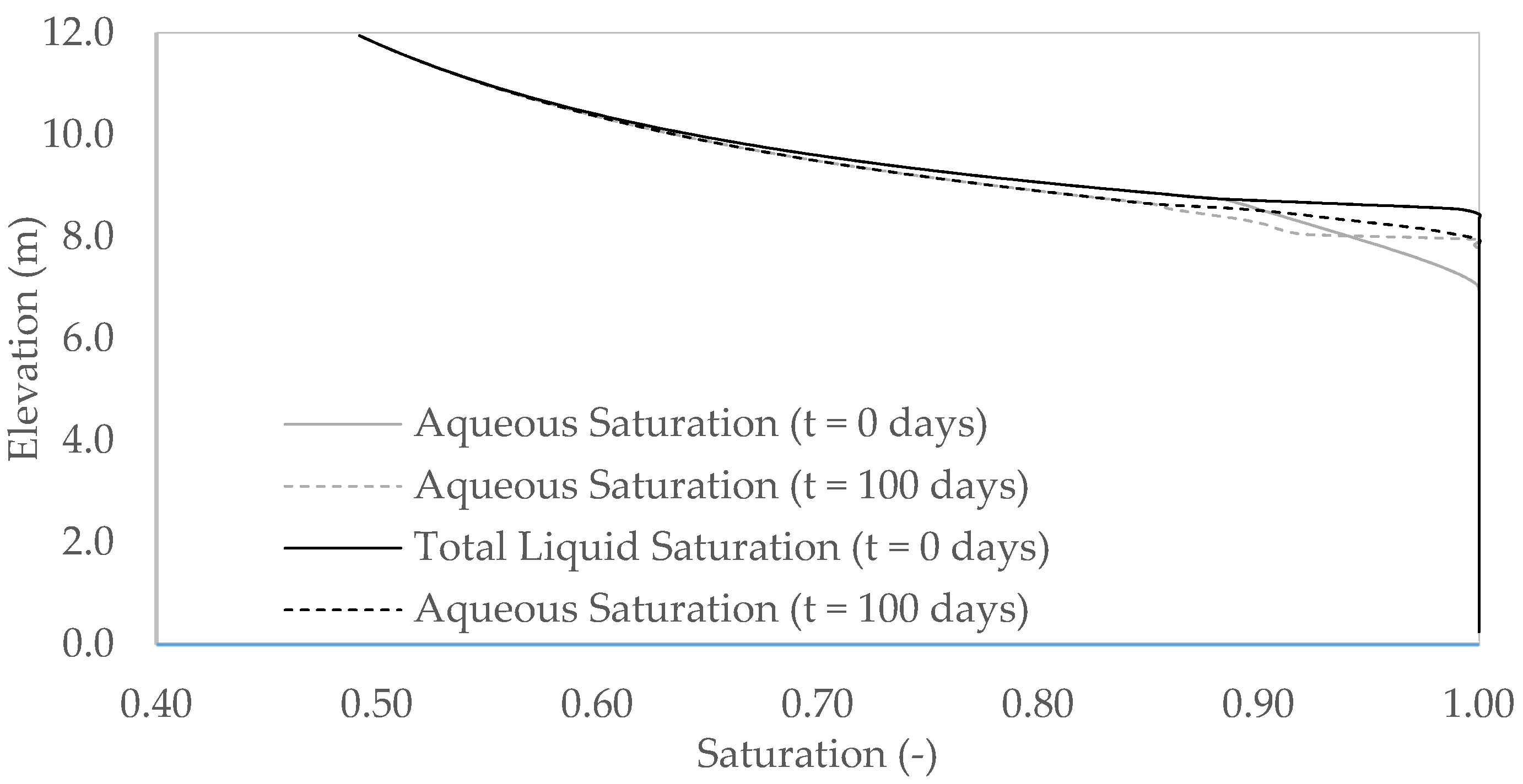
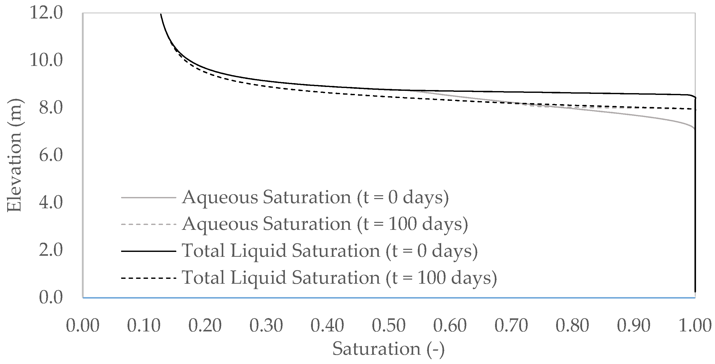
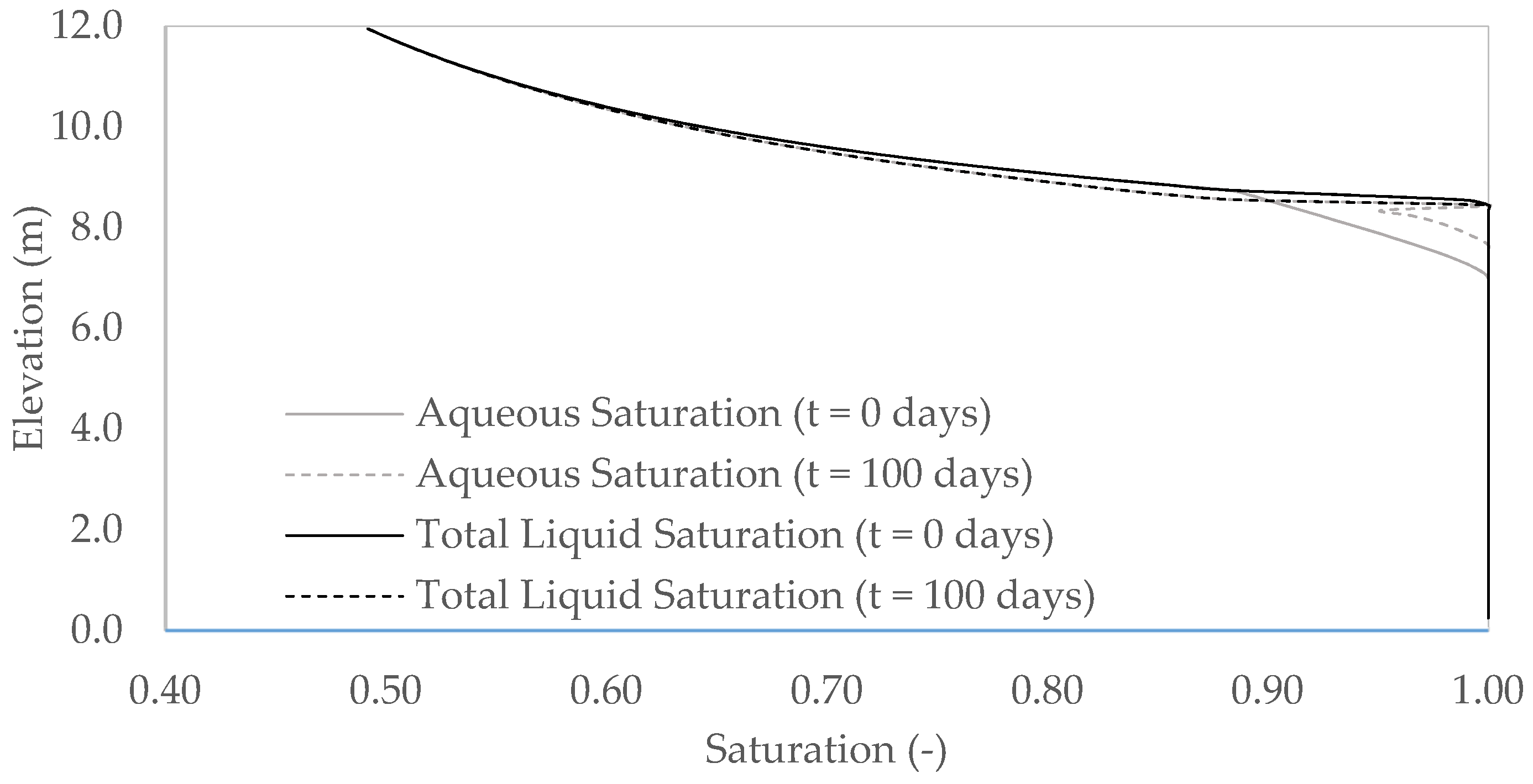
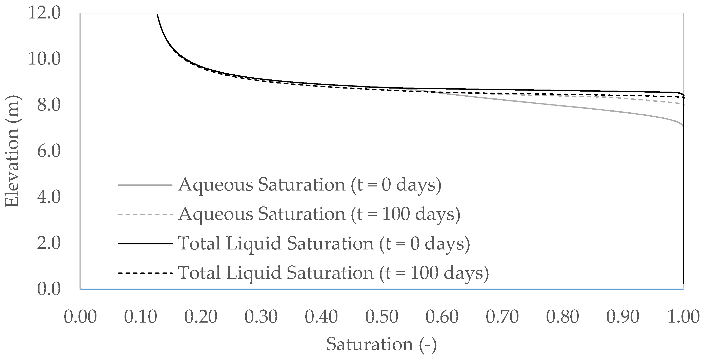
Figure 7, Figure 8, Figure 9, Figure 10 and Figure 11 show the simulation results of the initial (0 days) and final (100 days) aqueous and LNAPL saturations for both soils under 24.93 kPa in three different tip tube positions (TE2 = 7.05 m, TE6 = 7.95 m, and TE8 = 8.25 m) in the surrounding area of the well. The initial aqueous and total liquid saturation are denoted with continuous lines, while final aqueous and total liquid saturations are shown with dashed lines. Once the total liquid saturation represents the sum of oil and water saturation, the oil saturation can be obtained by subtracting the aqueous from total liquid saturation.
In Figure 7 (silty sand) and Figure 8 (oxisol), the tip tube was positioned at TE2 (7.05 m), where the interface between water and the LNAPL free phase was. After 100 days, an oil extraction of 0.1 m3 and 13.8 m3, respectively, could be verified for silty sand and oxisol. Thereby, the LNAPL thickness in the silty sand soil was 1.6 m, whereas this value in oxisol was 1.4 m. Regarding LNAPL saturation, in silty sand soil, a maximum value of 0.09 was observed, while in oxisol, LNAPL saturation reached a maximum of 0.37. Therefore, the tip tube positioning at the water–oil interface (TE2) caused almost no change in oil thickness and saturation near the well, but water flux into the extraction well was high.
In Figure 9 and Figure 10, saturation results for a tip tube location of TE6 (7.95 m) can be seen, which was inside the LNAPL layer. A total of 0.19 m3 of oil in silty sand was extracted, reducing the LNAPL thickness in soil near the well from 1.72 m to 0.8 m, while in oxisol, we recovered around 14 m3, and its oil thickness was 0.3 m adjacent to the well, having extracted a smaller volume of water than in TE2.
Figure 11 and Figure 12 depict the saturation results for a tip tube located in TE8 (8.45 m)—the interface between oil and air. In this MPE configuration (oil–air interface), the simulations predicted an oil extraction of 0.17 m3 and a reduction in LNAPL thickness of 0.92 m for silty sand. For oxisol, the extraction of oils was 7.0 m3, while the reduction in LNAPL thickness was 1.42 m. With respect to saturation, the maximum LNAPL saturation decreased to 24% in silty sand and 73% in oxisol. It can be seen that this configuration brought better results compared to the tip tube positioning at the oil–water interface, but it was less efficient than the tip tube positioned within the free phase.
Overall, the results from different tip tube locations indicate that the highest LNAPL saturation was around the interface between air and oil phases, decreasing rapidly above this boundary and more gradually below. In terms of oil recovery, the tip tube positioning, which yielded the greatest reduction of LNAPL thickness, was TE6, located inside the oil layer. A TE2 location, the US Army’s [8] recommended location, did not provide great values of oil recovery, and was considered the least effective in present simulations. In addition, the amount of water extracted was still considerable, increasing treatment costs. Despite TE8, the USEPA’s [7] recommended location, being adjacent to the highest LNAPL saturation location, the unsaturated zone made a limited contribution to LNAPL flow, making extraction less efficient. These results corroborated those found by Matos de Souza et al. [16] who, with different system configurations, porous media and contaminants, achieved greater oil removal with the tip tube between the fluid interfaces (in the oil phase).
3.4. LNAPL Saturation in Soil Profile and Extraction Radius of Influence
For oil saturation analysis before and after the application of the MPE technique and the possible definition of an influence radius for each well, we defined a set of vacuum and tip tube positions, and developed the simulation for the same 100 days of extraction. The applied vacuum of 24.93 kPa (VA7) and the tip tube position at TE6 (z = 7.95 m) at r = 0 were defined. This configuration was considered to have the appropriate performance in terms of the LNAPL extraction rate, preventing an excess of water and air extraction.
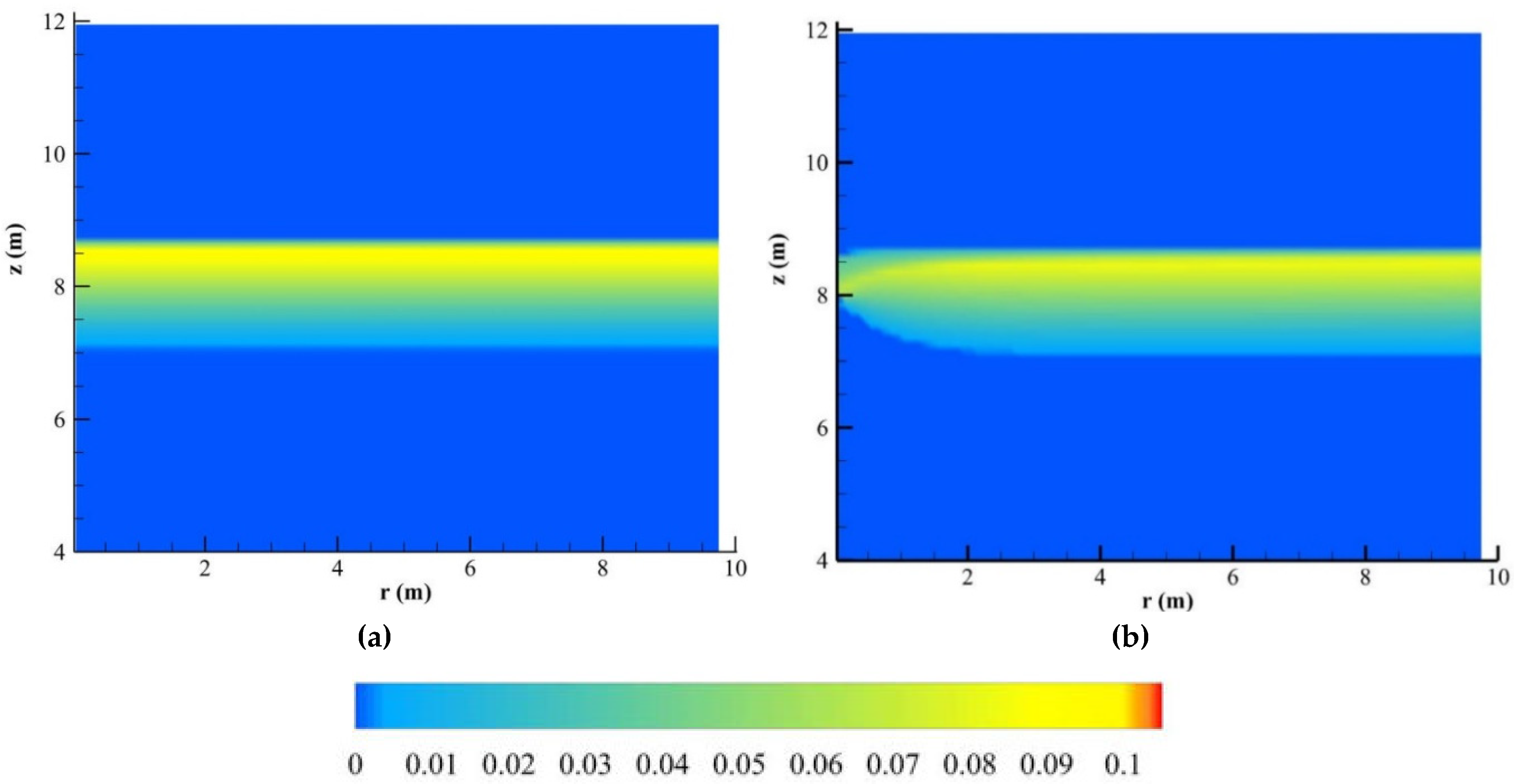
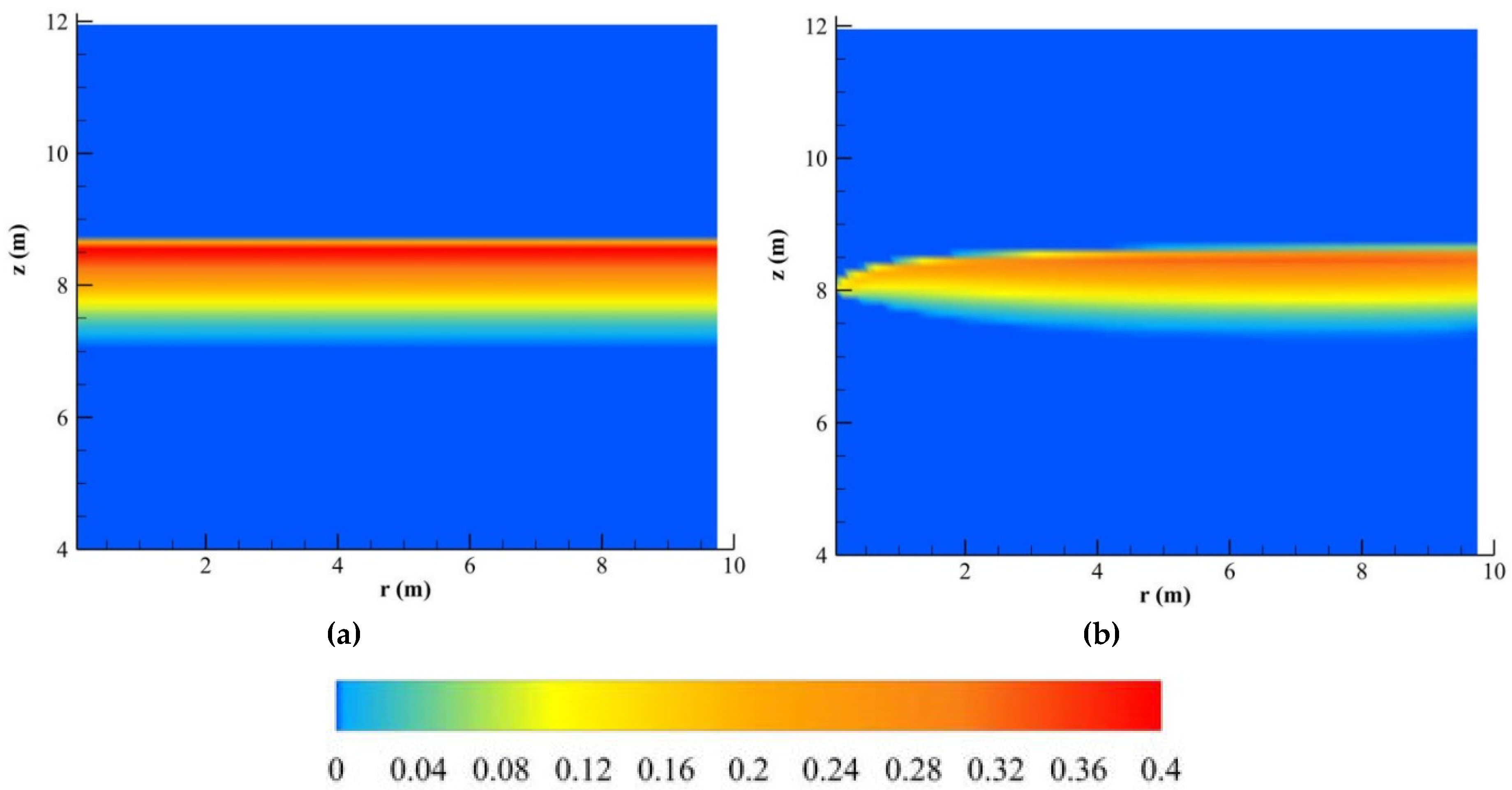
Figure 13 and Figure 14 show the results of the initial saturation profiles (a) and after 100 days of diesel extraction (b) of diesel oil thickness along the horizontal direction of silty sandy and oxisol, respectively. As noted earlier, the total amount of diesel in the silty soil model domain prior to extraction was approximately three times less than oxisol (12.480 kg and 38.092 kg, respectively). In addition, LNAPL saturation at the subsurface varies with depth and depends on capillary pressures, with maximum LNAPL saturation near the oil–air interface [34,40].
After 100 days, the total amount of oil extracted for the silty soil was 156 kg—a reduction of 1.25% of the total oil. For oxisol, the simulation indicated an amount of extracted oil of 11,887 kg, accounting for 31.2% oil removal in the domain. These results were mainly influenced by the transmissivity of the soils caused by the difference in their characteristics in pore size distribution, identified by the van Genuchten parameters and hydraulic conductivity.
Subsequently, the influence radius was evaluated, under the same conditions as previously established, for oil removal in both soils. The objective was to identify the distance in the –r direction from the vacuum tip tube location, where the effects of extraction from this well did not directly affect the oil thickness. In other words, this location in the –r direction may be indicated by the thickness of the vertical oil, water, and air profiles that are closer to the initial condition in the porous media, for example. In terms of LNAPL saturation in a porous media, the influence radius was defined for this study as the first position in the horizontal direction –r where the soil hydrocarbon thickness (Do) was 80% of the value prior to vacuum application. Defining a radius of influence can help to identify factors such as the distance between extraction wells or even to determine whether the technique is appropriate in a given contamination. The influence radius varies over the vacuum application time as proposed by Matos de Souza [30]. However, in the present study, only the influence radius with the same 100 days of extraction was evaluated.
The analysis resulted in a radius of influence of 1.15 m for silty sand and 5.25 m for oxisol. These results might lead to a possible incompatibility of the silty soil with MPE technique, since the results of extraction rates and reduction of oil present in the pores obtained with the model were low, even with a high free phase thickness detected in the well. This might show the need for a more complex extraction structure with a large number of wells, incurring high costs in the process. Regarding oxisol, under these conditions, this soil seemed quite suitable for the use of the technique, due to the high level of fluid extraction even when the applied vacuum was considered low.
3.5. Considering Residual and Entrapped LNAPL
Thus far, the results have disregarded the residual and entrapped LNAPL that were formed from the vacuum application. Disregarding this factor might lead to the overestimation of fluid extraction in the model, generating distorted predictions. Thus, other simulations were realized using the same MPE configuration as the previous step, considering the residual and entrapped effective maximum saturation (and , respectively) factors.
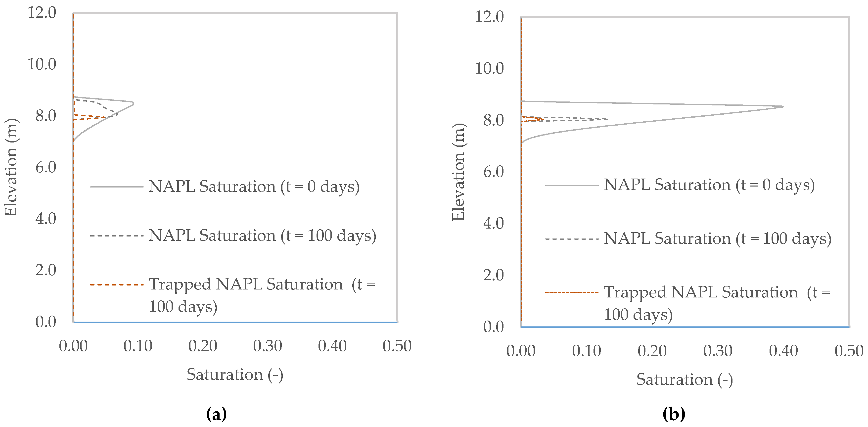
Figure 15 shows the free trapped LNAPL saturation profile resulting from the LNAPL thickness in the 1.50 m well at the initial condition (t = 0 days) and after 100 days of extraction near the well in silty sand (a) and oxisol (b), considering and were equal to 0.3.
Adjacent to the soil, a smaller amount of free LNAPL in the well was estimated when including trapped LNAPL, with the predicted volume of free LNAPL being 82.5% and 74.7% of the total LNAPL volume in silty sand and oxisol, respectively. The amount of trapped LNAPL decreased with increasing elevation in the soil, approaching zero as it neared the oil–air interface.
This presence of trapped LNAPL tended to reduce the predicted LNAPL transmissivity compared to when no trapped LNAPL was considered. This is what can be observed in Table 3, which presents the results of fluid extraction after the application of MPE in both soils. It shows LNAPL saturation when there was no residual or trapped LNAPL (case I); in other words, when all LNAPL was considered free and the expected results of free (mobile) and immobile (residual and entrapped) LNAPL, considering different and values (case II, case III and case IV).
As can be seen, the consideration of the factors and in both soils caused considerable changes in fluid extraction values with the progressive increase of these factors. In both soils, the recovery of LNAPL and water was reduced even though we applied the same extraction conditions. In silty sand, there was a reduction of 9.52% (case II), 13.25% (case III), and 15.47% (case IV) compared to the condition without trapped LNAPL. Meanwhile, in oxisol, this reduction was 5.96% (case II), 11.80% (case III), and 17.16% (case IV).
Several studies have discussed the consequences of disregarding the effects of oil trapping by water in porous media. Parker [3] verified experimentally that, in a hysteretic model, oil variation due to water level oscillation was estimated at two-thirds of the oil mass being trapped by water, concluding that a non-hysteretic model could overestimate the oil extraction from the porous media and drastically affect oil extraction techniques. Furthermore, it could be stated that even with small values of residual and entrapped LNAPL generated by the vacuum application, transmissivity reduction was expected, and therefore it was important to consider this immobile LNAPL when managing contamination extraction from wells. In addition, in relation to the vacuum applied to phase mass extraction, high vacuums cause discontinuities and a greater movement of water flow in the media, causing greater entrapment of LNAPL [38].
3.6. Bioslurping Influence in Dissolution and Volatilization Phases
An increase in immobile LNAPL in the porous media—due, for example, to water level variation, or as in the case of this extraction well vacuum application—does not only affect the transmissivity of the fluids, as seen above, but this immobile LNAPL also forms a potential source of long-term LNAPL in groundwater [41]. From this consideration, the effects of a bioslurping extraction well in the distribution of LNAPL concentrations along the porous media profile, as well as how vacuum trapping LNAPL influences the dissolution and volatilization of the present compounds, were analyzed.
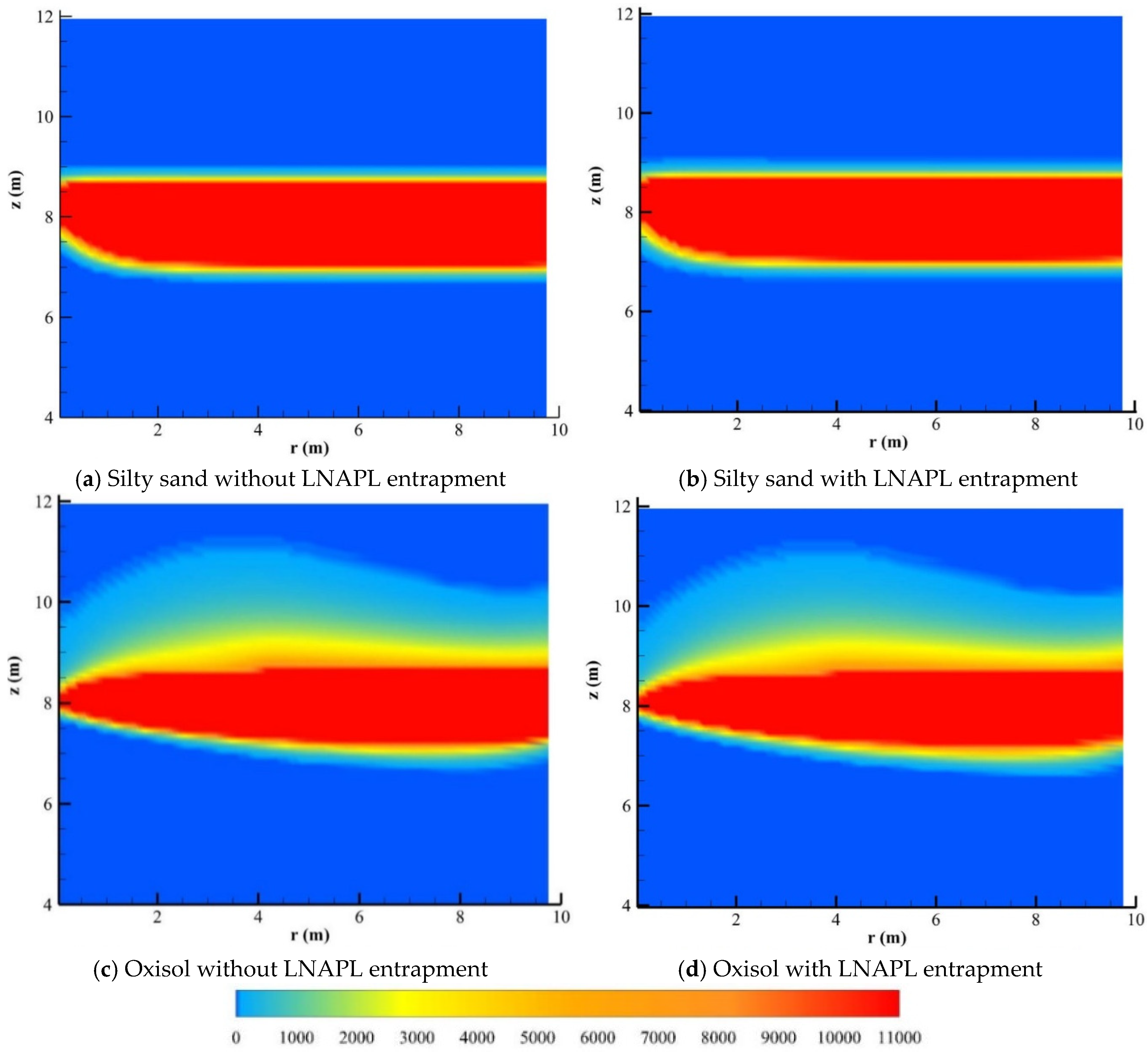
The concentration profile of diesel oil in the initial aqueous phase comprises 1.72 m oil thickness with a constant concentration of 11,000 ppm. For this, simulations were performed under the same conditions as the previous step system over 100 days (24 kPa vacuum pressure and z = 7.95 m tip tube) and with the dispersive conditions of the contaminants presented in Table 3. Figure 16 shows the simulation response of the MPE system in the concentration, in ppm, of the diesel compounds dissolved in the aqueous phase in both soils.
First, it is worth noting the difference in the effects that the MPE system had on silty sand and oxisol. In silty sand, not only were the volumes of the extracted fluids low, as seen before, but also the applied vacuum had effects on extraction. We observed that less than 0.5 m of dissolved concentrations in groundwater formed below the free phase and dissolved in aqueous saturation just above the oil thickness in the soil. Thus, it was concluded that this low transmissivity of the porous media, besides affecting the recovery of fluids through the extraction well, also affected the dispersion of contaminants. The simulation shows that, despite the low recoverability of the porous media and possible unfeasibility of the MPE technique in silty sand soil, LNAPL presented in a free form also had difficulty dispersing in the groundwater and air present in the soil pores, retaining more contamination.
Regarding oxisol, a clear effect of the applied technique was perceived, both in the recovery of dissolved phase near the extraction well, containing the advance of the plume, as well as the greater dispersion of contaminants due to its volatilization, probably facilitating the treatment of volatile compounds. This can easily be seen in the curve that volatile compounds form near the extraction well. Even though the goal of bioslurping is the maximized recovery of the oil phase, it is very important to understand that the removal of dissolved and volatilized phases is part of the technique, which uses the elements of bioventing and free pump-and-treat techniques, simultaneously recovering free products and causing a bioremediation of the vadose zone [8,10].
Regarding the consideration of and , with both factors being 0.3, we can see in Figure 16 a small variation in the diesel oil concentrations in the aqueous saturation of both soils. A higher concentration was observed in simulations considering the LNAPL trapped phase, which is represented by the amount of diesel oil that has been extracted from the media in a dissolved form or steam. Disregarding the factors and , the diesel extraction was 4 kg and 362 kg for silty sand and oxisol, respectively. However, when considering trapping, despite the lower water extraction and virtually unchanged vapor extraction (as shown in Table 3), the diesel masses extracted from silty sand and oxisol were 12 kg and 413 kg; i.e., the groundwater and air concentrations were higher considering the immobile LNAPL in the simulation.
4. Conclusions
The implementation of the MPE technique in a bioslurping configuration is widely used for the remediation of LNAPL-contaminated areas, even with uncertainties related to its application. Thus, this work presented results from a series of simulations using a numerical model to evaluate the technique’s application in a hypothetical diesel oil contamination scenario. The physical and hydraulic characteristics of two Brazilian soils (silty sand and oxisol) were used in simulations, allowing the evaluation of the differences between the soils, the extraction well configurations, and the behavior of the contaminant in porous media.
The van Genuchten α parameter from each soil water retention curve (SWRC) and the saturated hydraulic conductivity were important to determine the contaminant behavior. These parameters were the ones that most affected the extraction of fluids. The applied vacuum and tip tube position directly influenced the amount of slurped contaminant. The ideal position for maximizing LNAPL extraction in the soil is within the oil layer in the well. After 100 days of extraction, the reduction in LNAPL was quite different between the two soils, with higher fluid volumes and higher diesel oil removal efficiency in the oxisol. In addition, the consideration of immobile LNAPL in simulations yielded important results, and its consideration in models may be important to reduce errors in contaminant recovery predictions. Finally, regarding dissolution and volatilization, the mass transfers were different according to each porous media. From the simulations performed, the oxisol seemed to be appropriate for the application of MPE, whereas the application of the technique in silty sand did not seem to be feasible.
Thus, multiphase models could be used for this type of analysis if they consider the characteristics of the porous media and the dynamics of LNAPL contaminants, which STOMP has been capable of. Analyses such as these are important when LNAPL is redistributed by the vadose zone, by changes in the water table, or also by the use of well extraction techniques. The model can simulate, in addition to the behavior of the contaminant in the porous media during phase changes from the application of the technique, the recovery rates of the fluids and may help to predict the treatment time of the site. Field scale experiments are being performed to evaluate the model, considering other aspects that were not approached in this study.
Author Contributions
Conceptualization, S.F.B. and R.T.S. and M.C.B.; methodology, S.F.B. and R.T.S. and M.C.B.; software, S.F.B. and R.T.S.; validation, S.F.B. and R.T.S.; formal analysis, S.F.B. and R.T.S.; investigation, S.F.B. and R.T.S.; resources, S.F.B. and R.T.S.; data curation, S.F.B. and R.T.S.; writing—original draft preparation, S.F.B. and R.T.S.; writing—review and editing, S.F.B. and R.T.S. and M.C.B.; visualization, S.F.B. and R.T.S. and M.C.B.; supervision, M.C.B.; project administration, M.C.B.
Funding
This research was funded by Conselho Nacional de Desenvolvimento Científico e Tecnológico (CNPq) and Coordenação de Aperfeiçoamento de Pessoal de Nível Superior (CAPES).
Acknowledgments
This study was financed in part by the Coordenação de Aperfeiçoamento de Pessoal de Nível Superior—Brasil (CAPES)—Finance Code 001. The authors are grateful to the Brazilian Council of Technological and Scientific Development (CNPq) for the research scholarship conceived, and to the technical staff of the COPPE’s Geotechnical Laboratory.
Conflicts of Interest
The authors declare no conflict of interest.
References
- Huntley, D.; Beckett, G.D. Persistence of LNAPL sources: Relationship between risk reduction and LNAPL recovery. J. Contam. Hydrol. 2002, 59, 3–26. [Google Scholar] [CrossRef]
- Newell, C.J.; Acree, S.D.; Ross, R.R.; Huling, S.G. Light nonaqueous phase liquids. In US EPA: Ground Water Issue; EPA/540/S-95/500; US EPA: Washington, DC, USA, 1995; p. 28. [Google Scholar]
- Parker, J.C. Multiphase flow and transport in porous media. Rev. Geophys. 1989, 27, 311–328. [Google Scholar] [CrossRef]
- Mercer, J.W.; Cohen, R.M. A review of immiscible fluids in the subsurface: Properties, models, characterization and remediation. J. Contam. Hydrol. 1990, 6, 107–163. [Google Scholar] [CrossRef]
- Miller, C.T.; Christakos, G.; Imhoff, P.T.; Mcbride, J.F.; Pedit, J.A.; Trangenstein, J.A. Multiphase flow and transport modeling in heterogeneous porous media: Challenges and approaches. Adv. Water Resour. 1998, 21, 77–120. [Google Scholar] [CrossRef]
- Sookhak Lari, K.; Davis, G.B.; Johnston, C.D. Incorporating hysteresis in a multi-phase multi-component NAPL modelling framework; a multi-component LNAPL gasoline example. Adv. Water Resour. 2016, 96, 190–201. [Google Scholar] [CrossRef]
- USEPA (U.S. Environmental Protection Agency). Multi-Phase Extraction: State of the Practice; EPA-542-R-99-004; Office of Solid Waste and Emergency Response: Cincinnati, OH, USA, 1999.
- US ARMY. Multi-Phase Extraction—Engineering and Design; EM 1110-1-4010; US Army Corps of Engineers: Washington, DC, USA, 1999.
- Place, M.C.; Coonfare, C.T.; Chen, A.S.C.; Hoeppel, R.E.; Rosansky, S.H. Principles and Practices of Bioslurping, 1st ed.; Battelle Press: Columbus, OH, USA, 2001. [Google Scholar]
- Miller, R.R. Bioslurping. In GWRTAC Technology Overview Report; TO-96-05; Ground-Water Remediation Technologies Analysis Center: Pittsburgh, PA, USA, 1996. [Google Scholar]
- Kittel, J.A.; Hinchee, R.E.; Hoeppel, R.; Miller, R. Bioslurping—Vacuum-enhanced free product recovery coupled with bioventing: A case study. In Proceedings of the 1994 Conference on Petroleum Hydrocarbons and Organic Chemicals in Ground Water: Prevention, Detection, and Remediation, Houston, TX, USA, 2–4 November 1994; pp. 255–270. [Google Scholar]
- Colombo, L.; Alberti, L.; Mazzon, P.; Formentin, G. Transient Flow and Transport Modelling of an Historical CHC Source in North-West Milano. Water 2019, 11, 1745. [Google Scholar] [CrossRef]
- Ebrahimi, F.; Lenhard, R.J.; Nakhaei, M.; Nassery, H.R. An approach to optimize the location of LNAPL recovery wells using the concept of a LNAPL specific yield. Environ. Sci. Pollut. Res. 2019. [Google Scholar] [CrossRef]
- Gabr, M.A.; Sharmin, N.; Quaranta, J.D. Multiphase Extraction of Light Non-aqueous Phase Liquid (LNAPL) Using Prefabricated Vertical Wells. Geotech. Geol. Eng. 2013, 31, 103–118. [Google Scholar] [CrossRef]
- Sookhak Lari, K.; Johnston, C.D.; Rayner, J.L.; Davis, G.B. Field-scale multi-phase LNAPL remediation: Validating a new computational framework against sequential field pilot trials. J. Hazard. Mater. 2018, 345, 87–96. [Google Scholar] [CrossRef]
- de Souza, M.M.; Oostrom, M.; White, M.D.; da Silva, G.C.; Barbosa, M.C. Simulation of Subsurface Multiphase Contaminant Extraction Using a Bioslurping Well Model. Transp. Porous Med. 2016, 114, 649–673. [Google Scholar] [CrossRef]
- Lenhard, R.J.; Oostrom, M.; Dane, J.H. A constitutive model for air–NAPL–water flow in the vadose zone accounting for immobile, non-occluded (residual) NAPL in strongly water-wet porous media. J. Contam. Hydrol. 2004, 71, 261–282. [Google Scholar] [CrossRef] [PubMed]
- Huang, Y.F.; Huang, G.H.; Chakma, A.; Maqsood, I.; Chen, B.; Li, J.B.; Yang, Y.P. Remediation of Petroleum-contaminated Sites through Simulation of a DPVE-aided Cleanup Process: Part 1. Model Development. Energy Source Part A 2007, 29, 347–366. [Google Scholar] [CrossRef]
- Qin, X.S.; Huang, G.H.; Zeng, G.M.; Chakma, A. Simulation-based optimization of dual-phase vacuum extraction to remove nonaqueous phase liquids in subsurface. Water Resour. Res. 2008, 44, W04422. [Google Scholar] [CrossRef]
- White, M.D.; Oostrom, M. STOMP—Subsurface Transport Over Multiple Phases; Version 4.0; User’s Guide; PNNL-15782; Pacific Northwest National Laboratory, EUA: Richland, WA, USA, 2006.
- White, M.D.; Oostrom, M.; Rockhold, M.L.; Rosing, M. Scalable Modeling of Carbon Tetrachloride Migration at the Hanford Site Using the STOMP Simulator. Vadose Zone J. 2007, 7, 654–666. [Google Scholar] [CrossRef]
- Yoon, H.; Oostrom, M.; Wietsma, T.W.; Werth, C.J.; Valocchi, A.J. Numerical and experimental investigation of DNAPL removal mechanisms in a layered porous medium by means of soil vapor extraction. J. Contam. Hydrol. 2009, 109, 1–13. [Google Scholar] [CrossRef]
- Oostrom, M.; Hofstee, C.; Wietsma, T.W. Behaviour of a Viscous LNAPL Under Variable Water Table Conditions. Soil Sediment Contam. 2006, 15, 543–564. [Google Scholar] [CrossRef]
- ABNT (Brazilian Association of Technical Standards). NBR 7181: Soil—Grain size analysis (in Portuguese); ABNT: Rio de Janeiro, Brazil, 1984. [Google Scholar]
- ABNT (Brazilian Association of Technical Standards). NBR 6508: Gravel Grains Retained on the 4.8 mm Mesh Sieve—Determination of the Bulk Specific Gravity (in Portuguese); ABNT: Rio de Janeiro, Brazil, 1984. [Google Scholar]
- van Genuchten, M.T.H. A closed-form equation for predicting the hydraulic conductivity of unsaturated soils. Soil Sci. Soc. Am. J. 1980, 44, 892–898. [Google Scholar] [CrossRef]
- Coelho, C.R.B. Theoretical and Experimental Study of Water Flow and Equilibrium and Non-Equilibrium Solute Transport in Tropical Soils (in Portuguese). Ph.D. Thesis, Federal University of Rio de Janeiro, Rio de Janeiro, Brazil, 2016. [Google Scholar]
- ASTM D7042-16e3. Standard Test Method for Dynamic Viscosity and Density of Liquids by Stabinger Viscometer (and the Calculation of Kinematic Viscosity); ASTM International: West Conshohocken, PA, USA, 2016. [Google Scholar]
- ASTM D1331-14. Standard Test Methods for Surface and Interfacial Tension of Solutions of Paints, Solvents, Solutions of Surface-Active Agents, and Related Materials; ASTM International: West Conshohocken, PA, USA, 2014. [Google Scholar]
- de Matos Souza, M. Using the STOMP Simulator to Assess Bioslurping Recovery and Remediation Processes of Light Hydrocarbons in Contaminated Areas. Ph.D. Thesis, Federal University of Rio de Janeiro, Rio de Janeiro, Brazil, 2015. [Google Scholar]
- White, M.D.; Oostrom, M. STOMP-Subsurface Transport over Multiple Phases—Version 2.0—Theory Guide; Pacific Northwest National Laboratory, EUA: Richland, WA, USA, 2000.
- Sookhak Lari, K.; Davis, G.B.; Rayner, J.L.; Bastow, T.P.; Puzon, G.J. Natural source zone depletion of LNAPL: A critical review supporting modelling approaches. Water Res. 2019, 157, 630–646. [Google Scholar] [CrossRef]
- White, M.D.; Bacon, D.H.; White, S.K.; Zhang, Z.F. Fully coupled wells models for fluid injection and production. Energy Procedia 2013, 37, 3960–3970. [Google Scholar] [CrossRef]
- Lenhard, R.J.; Parker, J.C. Estimation of free hydrocarbon volume from fluid levels in monitoring wells. Ground Water 1990, 28, 57–67. [Google Scholar] [CrossRef]
- Mitchell, J.K.; Soga, K. Fundamentals of Soil Behaviour, 3rd ed.; John Wiley & Sons: Hoboken, NJ, USA, 2005; pp. 196–206. [Google Scholar]
- Ferreira, M.M.; Fernandes, B.; Curi, N. Mineralogia da fração argila e estrutura de latossolos da região sudeste do Brasil. Rev. Bras. Ciência Solo 1999, 23, 507–514. [Google Scholar] [CrossRef]
- Ferreira, M.M.; Fernandes, B.; Curi, N. Influência da mineralogia da fração argila nas propriedades físicas de latossolos da região sudeste do Brasil. Rev. Bras. Ciência Solo 1999, 23, 515–524. [Google Scholar] [CrossRef]
- Lenhard, R.J.; Rayner, J.L.; Davis, G.B. A practical tool for estimating subsurface LNAPL distributions and transmissivity using current and historical fluid levels in groundwater wells: Effects of entrapped and residual LNAPL. J. Contam. Hydrol. 2017, 205, 1–11. [Google Scholar] [CrossRef]
- Kacem, M.; Benadda, B. Mathematical Model for Multiphase Extraction Simulation. J. Environ. Eng. 2018, 144, 04018040. [Google Scholar] [CrossRef]
- Farr, A.M.; Houghtalen, R.J.; McWhorter, D.B. Volume Estimation of Light Nonaqueous Phase Liquids in Porous Media. Groundwater 1990, 28, 48–56. [Google Scholar] [CrossRef]
- ITRC (Interstate Technology & Regulatory Council). Evaluating LNAPL Remedial Technologies for Achieving Project Goals; Interstate Technology & Regulatory Council-LNAPL Teams: Washington, DC, USA, 2009. [Google Scholar]
Figure 1.
Multiphase extraction (MPE) system conceptual model.

Figure 2.
Soil water retention curve (SWRC) of silty sand soil.

Figure 3.
Soil water retention curve (SWRC) of oxisol.

Figure 4.
Slurped volume oil (a), water (b), and air (c) for 100 days as a function of vacuum pressure for extraction depending of the slurping tip tube positions z (TE1 = 6.85, TE2 = 7.05, TE3 = 7.25, TE4 = 7.55, TE5 = 7.75, TE6 = 7.95, and TE7 = 8.25 m) located in water (TE1), oil–water interface (TE2), oil (TE3, TE4, TE5, TE6, and TE7), air–oil interface (TE8), and air (TE9) in silty sand.

Figure 5.
Slurped volume oil (a), water (b), and air (c) for 100 days as a function of vacuum pressure for extraction depending of the slurping tip tube positions z (TE1 = 6.85, TE2 = 7.05, TE3 = 7.25, TE4 = 7.55, TE5 = 7.75, TE6 = 7.95, and TE7 = 8.25 m) located in water (TE1), oil–water interface (TE2), oil (TE3, TE4, TE5, TE6, and TE7), air–oil interface (TE8), and air (TE9) in oxisol.

Figure 6.
Oil extraction rate over time in 100 days of simulation using different vacuum pressures (a) Silty sand, (b) Oxisol (VA2 = 1.33, VA3 = 2.66, VA4 = 6.00, VA5 = 11.33, VA6 = 12.40, VA7 = 24.93, VA8 = 49.86, and VA9 = 66.26 kPa).
Figure 6.
Oil extraction rate over time in 100 days of simulation using different vacuum pressures (a) Silty sand, (b) Oxisol (VA2 = 1.33, VA3 = 2.66, VA4 = 6.00, VA5 = 11.33, VA6 = 12.40, VA7 = 24.93, VA8 = 49.86, and VA9 = 66.26 kPa).

Figure 7.
Aqueous and total saturation variation (initial and final) in TE2 under 24.93 kPa for silty sand.
Figure 7.
Aqueous and total saturation variation (initial and final) in TE2 under 24.93 kPa for silty sand.

Figure 8.
Aqueous and total saturation variation (initial and final) in TE2 under 24.93 kPa for oxisol.
Figure 8.
Aqueous and total saturation variation (initial and final) in TE2 under 24.93 kPa for oxisol.

Figure 9.
Aqueous and total saturation variation (initial and final) in TE6 under 24.93 kPa for silty sand.
Figure 9.
Aqueous and total saturation variation (initial and final) in TE6 under 24.93 kPa for silty sand.

Figure 10.
Aqueous and total saturation variation (initial and final) in TE6 under 24.93 kPa for oxisol.
Figure 10.
Aqueous and total saturation variation (initial and final) in TE6 under 24.93 kPa for oxisol.

Figure 11.
Aqueous and total saturation variation (initial and final) in TE8 under 24.93 kPa for silty sand.
Figure 11.
Aqueous and total saturation variation (initial and final) in TE8 under 24.93 kPa for silty sand.

Figure 12.
Aqueous and total saturation variation (initial and final) in TE8 under 24.93 kPa for oxisol.
Figure 12.
Aqueous and total saturation variation (initial and final) in TE8 under 24.93 kPa for oxisol.

Figure 13.
Initial saturation profile (a) and after 100 days of diesel extraction (b) in silty sand.
Figure 13.
Initial saturation profile (a) and after 100 days of diesel extraction (b) in silty sand.

Figure 14.
Initial saturation profile (a) and after 100 days of diesel extraction (b) in oxisol.

Figure 15.
Free and entrapped LNAPL after 100 days of extraction: (a) silty sand; and (b) oxisol.

Figure 16.
Concentration of LNAPL in an aqueous phase in response to the MPE system simulation without and with LNAPL entrapment.
Figure 16.
Concentration of LNAPL in an aqueous phase in response to the MPE system simulation without and with LNAPL entrapment.


Table 1.
Porous media properties. LNAPL: light non-aqueous phase liquids.
| Parameters | Values | |
|---|---|---|
| Silty Sand | Oxisol | |
| Specific gravity (kg m−3) | 2747 | 2637 |
| Total porosity (–) | 0.49 | 0.49 |
| Sandy (%) | 65 | 75 |
| Silt (%) | 30 | 10 |
| Clay (%) | 5 | 15 |
| Water-saturated hydraulic conductivity (cm s−1) | 8.5 × 10⁻⁵ | 8.48 × 10⁻³ |
| van Genuchten α (m−1) | 1.31 | 2.77 |
| van Genuchten n (–) | 1.49 | 3.45 |
| Irreducible water saturation Θr (–) | 0.080 | 0.03 |
| Longitudinal dispersivity (m) | 0.056 | 0.056 |
| Transversal dispersivity (m) | 0.0056 | 0.0056 |
Table 2.
Diesel properties.
| Parameters | Values |
|---|---|
| LNAPL mass density (kg m−3) | 830 |
| LNAPL viscosity (Pa s) | 3.45 × 10⁻³ |
| Air–LNAPL interfacial tension (N m−1) | 0.028 |
| Air–water interfacial tension (N m−1) | 0.072 |
| LNAPL–water interfacial tension (N m−1) | 0.034 |
Table 3.
Fluids extraction after MPE application for different cases.
| Residual and Entrapped Oil Saturation Factor | Silty Sandy | Oxisol | ||||||
|---|---|---|---|---|---|---|---|---|
| Water Extraction (kg) | Oil Extracted (kg) | Air Extracted (kg) | Water Extraction (kg) | Oil Extracted (kg) | Air Extracted (kg) | |||
| Case I | 0 | 0 | 3.59 + 03 | 1.56E + 02 | 2.34E + 00 | 6.24E + 05 | 1.19E + 04 | 1.33E + 03 |
| Case II | 0.1 | 0.1 | 3.08E + 03 | 1.41E + 02 | 2.40E + 00 | 5.99E + 05 | 1.12E + 04 | 1.38E + 03 |
| Case III | 0.2 | 0.2 | 2.99E + 03 | 1.35E + 02 | 2.52E + 00 | 5.79E + 05 | 1.05E + 04 | 1.38E + 03 |
| Case IV | 0.3 | 0.3 | 2.95E + 03 | 1.32E + 02 | 2.59E + 00 | 5.65E + 05 | 9.85E + 03 | 1.38E + 03 |
© 2019 by the authors. Licensee MDPI, Basel, Switzerland. This article is an open access article distributed under the terms and conditions of the Creative Commons Attribution (CC BY) license (http://creativecommons.org/licenses/by/4.0/).
Share and Cite
MDPI and ACS Style
Bortoni, S.F.; Schlosser, R.T.; Barbosa, M.C. Numerical Modeling of Multiphase Extraction (MPE) Aiming at LNAPL Recovery in Tropical Soils. Water 2019, 11, 2248. https://doi.org/10.3390/w11112248
AMA Style
Bortoni SF, Schlosser RT, Barbosa MC. Numerical Modeling of Multiphase Extraction (MPE) Aiming at LNAPL Recovery in Tropical Soils. Water. 2019; 11(11):2248. https://doi.org/10.3390/w11112248
Chicago/Turabian StyleBortoni, Samanta Ferreira, Rodrigo Trindade Schlosser, and Maria Claudia Barbosa. 2019. "Numerical Modeling of Multiphase Extraction (MPE) Aiming at LNAPL Recovery in Tropical Soils" Water 11, no. 11: 2248. https://doi.org/10.3390/w11112248
Note that from the first issue of 2016, this journal uses article numbers instead of page numbers. See further details here.