Spatial and Temporal Variations in Water Quality and Land Use in a Semi-Arid Catchment in Bolivia

Abstract

Increasing pressures caused by human activities pose a major threat to water availability and quality worldwide. Water resources have been declining in many catchments during recent decades. This study investigated patterns of river water quality status in a peri-urban/rural catchment in Bolivia in relation to land use during a 26 year period. Satellite images were used to determine changes in land use. To assess water quality, data in the dry season from former studies (1991–2014), complemented with newly collected data (2017), were analysed using the National Sanitation Foundation-Water Quality Index method and the Implicit Pollution Index method. The highest rates of relative increase in land use area were observed for forest, urban, and peri-urban areas, whereas relative decreases were observed for water infiltration zones, bare soil, shrubland, and grassland areas. The water quality indices revealed clear water quality deterioration over time, and from catchment headwaters to outlet. Statistical analyses revealed a significant relationship between decreasing water quality and urban expansion. These results demonstrate the need for an effective control programme, preferably based on water quality index approaches as in the present study and including continuous monitoring of runoff water, mitigation of pollution, and water quality restoration, in order to achieve proper water management and quality.

1. Introduction

Human activities and climate change are imposing increasing pressures on water availability and quality worldwide. Land use changes have a significant impact on hydrological system components such as surface runoff, infiltration, and interflow [1]. The loss of pervious surfaces such as shrubland, water infiltration zones, grassland, and forest reduces water infiltration and increases the variation in water flow by causing high streamflow [2]. Assessing the impacts of land use and land cover changes on hydrology is the basis for watershed management and ecological restoration [3]. According to Giri and Qiu [4], water quality [5] in watersheds [6,7] is affected by changes in land use and cover, which result from the interaction between anthropogenic and natural drivers. Li et al. [8] found that in a basin in China, reaches of the river next to vegetated areas had lower levels of nutrients than reaches close to degraded land (bare land and urban land). Haidary et al. [9] made similar findings for some wetlands in Japan, whereas in the state of Ohio, USA, Tong and Chen [10] found a significant relationship between land use and in-stream water quality. In a watershed in California, Ahearn et al. [11] showed that land use exerts the greatest control over water quality through the relationship between increasing percentage of farmland cover and increased nutrient loading. Tu [12] demonstrated the ability of land use indicators to explain water quality variations across an urbanisation gradient in Massachusetts, whereas Chen et al. [13] identified significant associations between urban land use (the most disruptive land use type) and water quality-related parameters in a watershed in China.

Inadequate water supply and declining water quality have been a persistent problem in the Rocha River catchment in Cochabamba, central Bolivia, during the past 30 years. Ongoing urbanisation in Cochabamba has worsened water quality status of the river to the point that it is now commonly regarded as an open sewer. For that reason, a number of assessments have been carried out to evaluate water quality [14,15,16,17] through measuring environmental quality parameters and variations in the degree of organic pollution in catchments. The main parameters measured in these studies have been nitrates, chemical oxygen demand, biological oxygen demand, and dissolved oxygen, in order to assess organic pollution. Faecal coliforms, phosphate, suspended solids, total solids, temperature, turbidity, and pH have also been recorded to evaluate the degree of purity of water for mostly domestic uses. A general conclusion in such studies is that pollution levels in the Rocha River are increasing [18,19,20,21,22,23,24].

Water quality in water bodies is usually assessed by physicochemical and biological parameters, such as those listed above, that are directly associated with water use. However, water quality as a whole is not clearly defined by studying these parameters separately [25]. A more convenient alternative is the use of a water quality index (WQI), which is a single dimensionless number that describes water quality in a simple form by aggregating the value of selected measured parameters [26].

A formal definition of WQI was initially suggested by Horton [27]. Brown et al. [28,29] later included additive and multiplicative properties in the definition and Prati et al. [30] sought to develop an index as a numerical expression of degree of pollution. In a review of the creation and modification of WQI, Lumb et al. [31] described other improvements and alterations that have been suggested and introduced for developing WQI types over time. Using WQI, Şener et al. [32] evaluated water quality in a river basin in Turkey and found that it was poor/very poor in the north and south of the basin, whereas Ewaid and Abed [33] classified a river in Iraq as good for drinking. Kannel et al. [34] used WQI to evaluate spatial and seasonal changes in surface water quality in a river basin in Nepal, whereas Debels et al. [35] calculated WQI in order to characterise the spatial and temporal variability in surface water quality in a river basin in Chile on the basis of nine physicochemical parameters periodically measured in the basin. A WQI was also applied by Salcedo-Sánchez et al. [36] when evaluating spatial and temporal variations in groundwater quality in the urban area of an aquifer in Mexico.

In Bolivia, no previous peer-reviewed study has attempted to investigate the relationship between land use and water quality indices. At the same time, there is a lack of data from long-term environmental monitoring regarding water resources in the study area. Thus, the aim of the present study was to assess the impacts of land use on surface water quality on the basis of two WQI approaches: The National Sanitation Foundation Water Quality Index (NSF-WQI) and Prati’s Implicit Index of Pollution (IPI).

We took existing historical water quality data (dissolved oxygen, faecal coliforms, pH, biological oxygen demand, nitrate, phosphate, temperature, turbidity, and total solids) from previous individual studies and complemented these with up-to-date measurements on water samples from the catchment during dry seasons, covering a 26 year period (1991–2017). We analysed the complete dataset and used the WQIs to estimate water quality variations in river water in the catchment during dry seasons, when low-flow conditions generally occur and pollution is most severe. We used Landsat images to determine land use during the 26 year study period and compared variations in WQI values against changes in land use types, focusing on the impacts of urbanisation.

2. Materials and Methods

2.1. Study Area

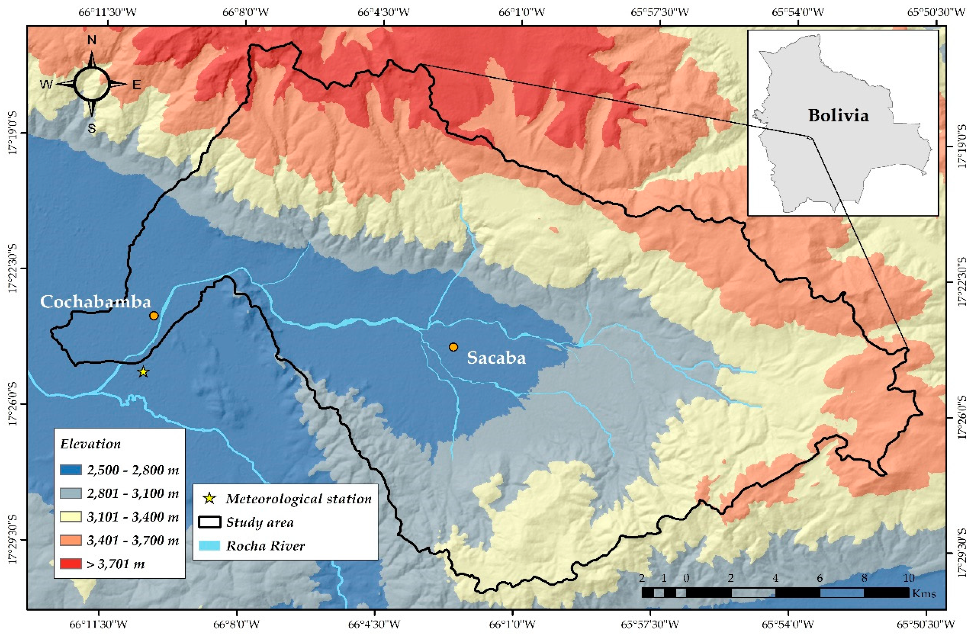
The Rocha River catchment is situated in the eastern Andes of Bolivia, with its outlet at the city of Cochabamba (17°20’–17°30’ S; 65°50’–66°10’ W). The catchment area is approximately 488 km². The population in the catchment was 530,258 in 1992 and 1,135,474 in 2012 [37], and it increased to an estimated 1,350,000 by 2017 [38]. Sacaba city is located near the centre of the catchment (Figure 1) and had 36,905 inhabitants in 1992, 172,466 in 2012, and 206,298 in 2017, giving an average population growth rate of 3.65% per year [38].

Temperature and precipitation at the outlet of the catchment during two 26 year periods are presented in Figure 2, 1991–2017 representing the period of the present study and 1964–1990 the preceding period. The data were recorded at a meteorological station at Cochabamba airport (17°24’58” S, 66°10’28” E, altitude 2548 m). The mean temperature was significantly higher (p < 0.0001) in the period 1991–2017 than in 1964–1990. Median annual temperature increased from 16.8 °C (1964–1990) to 17.8 °C (1991–2017), whereas the ranges in mean annual temperature were similar for the two periods—1.9 °C in 1964–1990 and 1.6 °C in 1991–2017. Median precipitation decreased (non-significantly) from 455 mm year⁻¹ in 1964–1990 to 421 mm year⁻¹ in 1991–2017 (Figure 2), whereas the range in precipitation was smaller in the latter period (265 mm) than in the former (435 mm). A general trend that emerged from comparison of the two 26 year periods was thus that the climate in the region has become warmer. The semi-arid climatic conditions in the area, generating low precipitation amounts during dry seasons and high amounts during wet seasons, greatly influence the variations in water quality in the river over the year [14]. The heavy summer rains during December–March [21] can decrease pollutant concentrations through dilution.

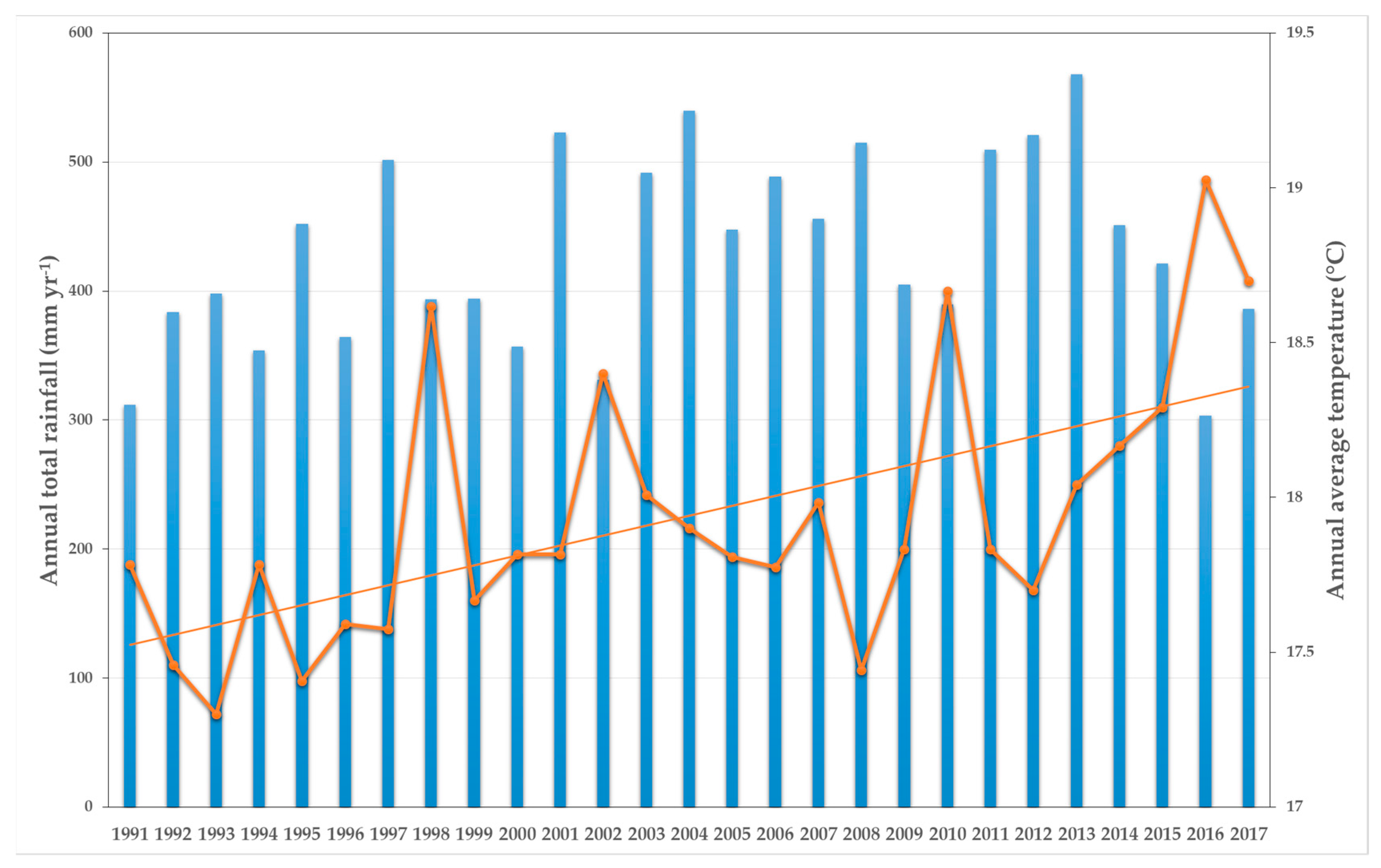
Yearly values of annual total rainfall and average temperature for the period 1991–2017 are presented in Figure 3. Rainfall in the period varied between 303 and 568 mm and temperature between 17.4 and 19.0 °C. There was a significant increase in temperature (p = 0.0023) over the total period.

The landscape is composed of mountains, hills, piedmonts, and valleys, with altitude ranging between 2500 and 3600 m [39]. In the piedmont area, the soil type is loam and silt loam, with low organic matter content and variable amounts of rock fragments in the soil matrix. Soil permeability is commonly high, but soil erosion still occurs as rill, pipe, and gully erosion. Depositional glacial tills (covered pediment) have finer soil texture and include locally poorly drained areas. Fine clay and clay loam texture with poor internal drainage is a common characteristic of soils with parent materials of alluvio-lacustrine origin [40]. The valley was formed from a tectonic graben filled by Quaternary deposits. The central area is a lagunary depression, occupying the lowest parts of the catchment, and the margins of the lagunary flats are almost level surfaces with slopes of less than 1%. The valley area is characterised by badlands and flatlands of alluvio-lacustrine origin. Fine-textured lacustrine sediments include isolated gravel channels, lenses, and sheets that conduct subsurface water flow, causing the formation of tunnels and pipes. Lacustrine sediments are very erodible silty and loamy materials, with weakly developed pedogenic features. A detailed description of the soil units and types can be found in Metternicht and Fermont [41].

According to Metternicht and Gonzalez [42], the natural vegetation in the catchment is mostly xeromorphic. The dominant plants in the natural flora are molle (Schinus molle), eucalyptus (Eucalyptus globulus), chilka (Baccharis latifolia), chacatea (Dodonaea viscosa), and suncho (Viguiera mandonii), associated with locust shrubs. Rainfed crops include maize (Zea mays), wheat (Triticum sativum), alfalfa (Medicago sativa), bean (Vicia faba), pea (Pisum sativum), onion (Allium cepa), and, to a lesser extent, quinoa (Chinchona amygdalifolia) [40]. Moreover, it is estimated that there are between 5000 and 7000 hectares of irrigated crops, mainly potatoes and various vegetables, which are irrigated with river water.

2.2. Land Use and Land Use Changes

Satellite images were used to study changes in land use during the 26 year study period (1991–2017). Landsat-5 Thematic Mapper (TM) images from 1991, 1997, and 2011 (paths 232 and 233, row 72) and 2005 (path 232, row 72) and Landsat-8 Operational Land Imager and Thermal Infrared Sensor (OLI/TIRS) images from 2014 and 2017 (paths 232 and 233, row 72), with general spatial resolution of 30 × 30 m with L1T (Standard Terrain Correction), were downloaded from the United States Geological Survey (USGS; http://glovis.usgs.gov). These images were chosen mainly because the dates of acquisition coincided with the dates of water quality sampling.

Landsat surface reflectance images were derived from the Landsat images. These images were already atmospherically corrected, but they needed to be re-projected to zone 19 in the Southern Hemisphere. The images were rectified to a common Universal Transversal Mercator (UTM) coordinate system (WGS 1984) based on a 1:50,000 scale topographical map. Each Landsat image was enhanced in ArcGIS 10.4, using standard deviation (2.5) linear contrast stretching and histogram equalisation to improve the image, in order to help identify ground truth for image classification. Different colour composites were employed for each set of images, and the best for performing analyses on Landsat 5 images were found to be bands 7, 4, and 2, whereas the best for performing analyses on Landsat 8 images were found to be bands 7, 5, and 3. Finally, principal component analysis (PCA) with all the bands per scene and band rationing operation was carried out with spectral index calculation to identify and differentiate the land uses. The Landsat images were classified, initially using the Iterative Self Organising (ISO) cluster unsupervised classification and thereafter the maximum likelihood classification algorithm. The ISO cluster unsupervised classification does not require prior knowledge of the study area, whereas the maximum likelihood classification does. Therefore, information generated in the ISO process was used, together with knowledge of the study area based on the experience of the people in charge of classification, to improve the maximum likelihood classification process.

However, the effect of topography made classification difficult, mainly for shadows, so to obtain better results for hillside and mountain areas, topography correction was used. Another drawback observed at the time of separation of the classes was that many mixed pixels were present due to the number of classes and the scope of the study area. Secondary information was used and field visits were made to solve this problem, which typically arises when classification depends on the spectral response of the Earth’s surface.

The number of land use classes used was increased from originally 5 (forest, crops, shrubland, water, and urban) to 10. This increased the degree of separability and therefore the progressive reduction of mixed pixels. The initial classes were differentiated by the ISO cluster unsupervised classification, whereas the other classes (bare soil, grassland, peri-urban, river, and infiltration zones) were derived after maximum likelihood classification. Results from former studies (e.g., [43]) also helped in the definition of classes, as did direct observations (rivers and lakes) and researcher experience and knowledge. When using data from former studies, the land use classes could not be verified in the field by field visits. Thus, the classification process was validated by accuracy assessment only for the most recent (current) data in the study.

Accuracy assessment was carried out by error matrices as cross tabulation of the land use map versus 100 ground control points per type (independent dataset samples) obtained by stratified random sampling in the field. The overall accuracy metric and the Kappa statistic were derived from the error matrices. Overall accuracy indicates the percentage of total pixels in the image that are correctly classified and Kappa (K) is a measure of agreement between predefined producer ratings and user assigned ratings [44]. It is calculated as [45]

$$K=P_{\left(A\right)}-P_{\left(E\right)}/1-P_{\left(E\right)}$$

(1)

where P_(A) is the observed proportion of agreement (i.e., the actual agreement) and P_(E) is the proportion of agreement that is expected to occur by chance.

Land use change was detected by area-based comparison to produce change information and thus interpret the changes more efficiently, taking advantage of ‘from-to’ information.

2.3. Data Collection and Sampling

Historical data on water quality and flow in the catchment between 1991 and 2014 were gathered from other studies (named ‘former’ in the following). Available physicochemical and biological water quality data for the years 1991, 1997, 2005, 2011, and 2014 were used in this study. Furthermore, in a complementary dataset (named ‘current’ in the following), water quality and flow parameters were measured in 2017, with particular focus on parameters for calculation of WQI.

The data used in the 1991 analysis were taken from Water Program [22], those in the 1997 analysis from Romero et al. [17], those for 2005 from the Department of Cochabamba Prefecture [16], those for 2011 from the General Comptroller of State [14], and those for 2014 from Sacaba´s Municipal Autonomous Government [15] and Mother Earth and Environment Direction [46]. These publications and reports were selected for the following reasons: (1) they have similar objectives regarding pollution in the Rocha River, (2) a wide range of water quality parameters were analysed, (3) they employ similar standard techniques for water quality sampling, and (4) the analyses were performed by the CASA (Water and Environmental Sanitation Center) laboratory, University Major of San Simon, Cochabamba city (1991, 1997, 2017) or by SPECTROLAB, Technical University of Oruro, Oruro city (2005, 2011, 2014).

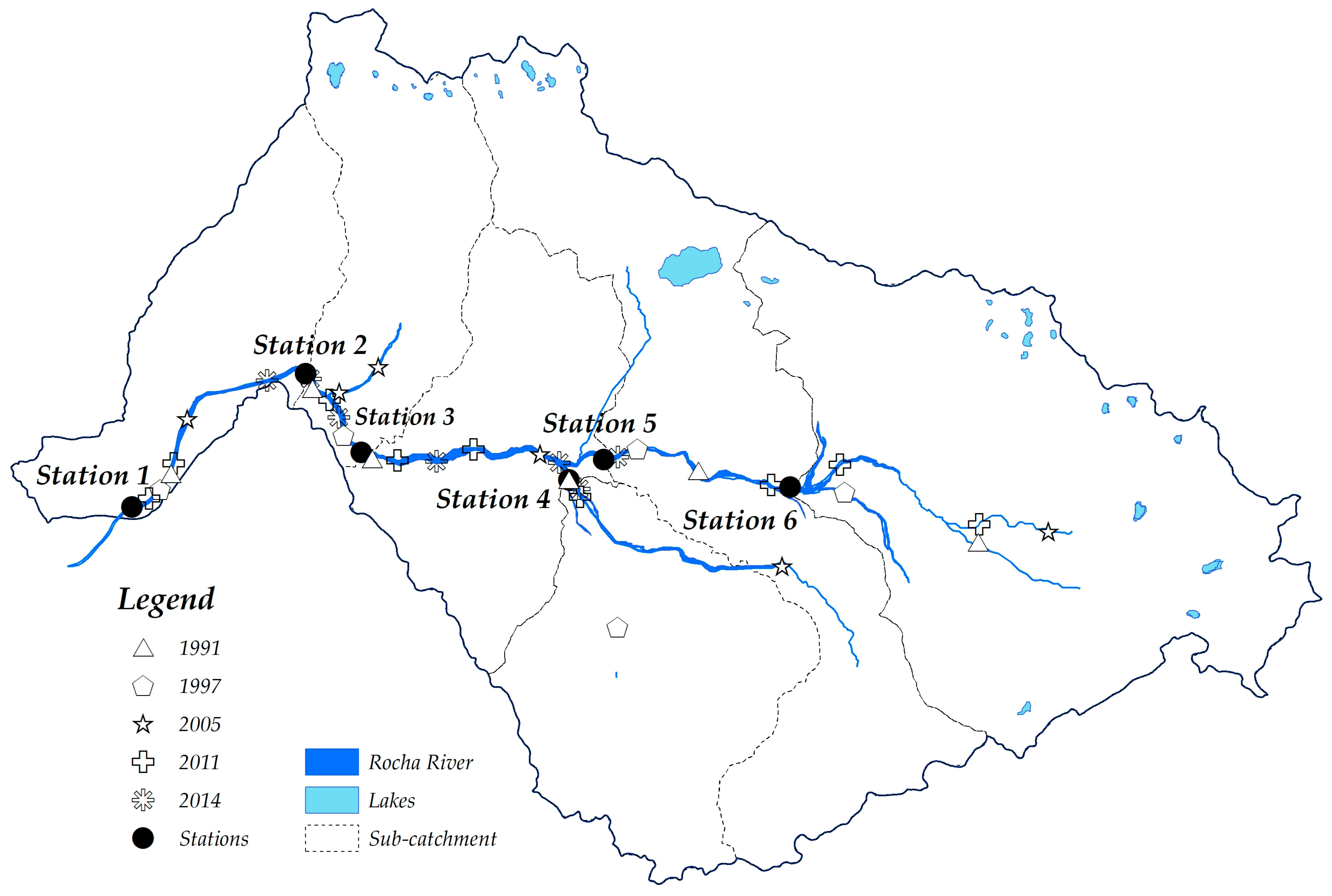
Six sampling stations were defined for data collection for the 2017 analyses (Figure 4). Definition was based on the underlying conditions that the sites were (a) considered to be representative of the study area with regard to land use types in the upstream contributing area and (b) related to a higher number of WQI-related parameters sampled in former studies and a higher frequency of sampling. Additional criteria considered when choosing the stations were access to the sites and number of contributing tributaries, as suggested by Chilundo et al. [47]. Sub-catchments corresponding to area of contribution of each of the six sampling stations were also delineated (Figure 4), using hydro-processing techniques in ArcGIS 10.4. Water quality samples and water flow points in the former dataset (Figure 4) were incorporated and related to the nearest downstream measurement station in the current data set (i.e., to station 1–6) in the WQI analyses.

A brief description of the six stations was made on the basis of field visits and observations. Station 1 is located at the catchment outlet, near the city airport, in an area classified as urban. It receives sewage water and the flow from upstream stations 2–6. Station 2 is located near paved areas under a bridge. Its surroundings are classified as peri-urban and urban, with some agricultural land present to the north. The land use in the area around station 3 is mainly peri-urban, with some agricultural land. Station 4 is located near the inlet of the southern tributary to the Rocha River. Discharge of raw domestic sewage water and effluent from some small industries was observed during field visits and the contributing area is urban, peri-urban, and agricultural (arable). Station 5 is located near the main residential area in Sacaba city and the land use is mainly peri-urban, with livestock and arable, and some urban land use in paved areas. Station 6 is located near a highly trafficked paved road, under a bridge and near a small urban area, but the contributing area is mainly used for agricultural purposes.

In order to maintain consistency throughout the whole dataset series from 1991 to 2017, data used in the 2017 analyses were sampled and analysed in accordance with techniques and methods used in the former studies, in particular Standard Methods for the Examination of Water and Wastewater by APHA [48] (1991, 1997, 2017) and Standard Methods for Water by ASTM [49] (2005, 2011, 2014). In general, sampling consisted of transferring single 1000 mL water samples from the midstream of the river to sterilised plastic bottles and acidifying the contents with nitric acid to pH <2. For bacteriological studies and biological and chemical oxygen demand, amber sterile glass bottles were used. Samples were transported to the laboratory and stored at 4 °C until analysis. Direct measurements in field 2017 included recording pH with a pH meter (ExStik pH100, Extech Instrument, Nashua, NH, USA), turbidity with a turbidity meter (HI93703, Hanna Instruments, Padova, Italy), and nitrates and phosphates with a spectrometer (Photometer YSI 9500, YSI Incorporated, Yellow Springs, OH, USA). The discharge measurements were made using a floating method and, more recently, with a Universal Current Meter (OTT series: 300801, OTT Hydromet GmbH, Kempten, Germany) designed for flow velocity measurements.

The laboratory methods used for determination of different water quality parameters in the former and current datasets, along with the units of measurement, are presented in

Table 1. Summary of laboratory techniques, standard methods used, and detection limits for determination of different parameters.

Parameter	Technique	Standard Method	Detection Limit
Dissolved oxygen	Membrane electrode Luminescence-based	SM4500-O C ASTM D888-05	0.05 mgO2/L 1 mgO2/L
Faecal coliforms	Membrane filter	SM 9222-D SM 9222-B	0 UFC/mL
pH	Electrometric	ASTM D 1293-99 4500-HB	0.01 pH 0.1 pH
Biological oxygen demand	Winkler dilution Dilution	SM 5210 B DIN 38409	2 mgO2/L 5 mgO2/L
Chemical oxygen demand	Dichromate oxidation	SM 5220 B ASTM D 1252-00	2 mgO2/L
Phosphates	Colorimetric	SM 2500-PO3 EPA 365.2	0.08 mgP/L 0.01 mgP/L
Nitrates	Cadmium reduction Colorimetric	SM 4500-NO3 DIN 38405	0.01 mgN–NO3/L
Turbidity	Nephelometric	2130 B	0.1 NTU
Total solids	Gravimetric—105 ˚C Colorimetric	SM 2540 B DIN 38409 H1	0.01 mg/L 1 mg/L

.

2.4. Water Quality Indices

Two WQIs were used—The National Sanitation Foundation Water Quality Index (NSF-WQI) and a modified short version by Romero et al. [17] of Prati’s Implicit Index of Pollution (IPI). They were applied in order to assess the current water quality status of the Rocha River and enable comparison with the water quality status reported in former studies. Samples (former and current) included in calculation of the WQIs were taken in the dry season, thus the effect of elements (nutrients or pollutants) can be considered to be at its maximum.

The NSF-WQI was developed by the National Sanitation Foundation of the United States of America using the Delphi method on the basis of nine parameters [28] with corresponding weights (

Table 2. Weighting values of parameters used to determine the National Sanitation Foundation Water Quality Index (NSF-WQI) (from Abbasi and Abbasi [50]).

Parameter	Weight
Dissolved oxygen	0.17
Faecal coliforms	0.16
pH Biochemical oxygen demand	0.11 0.11
Phosphates Nitrates	0.10 0.10
Delta temperature	0.10
Turbidity	0.08
Total solids	0.07

). These parameter values are measured and transferred to a weighting curve chart, where a numerical value of q_i is obtained. The mathematical expression for NSF-WQI is

$$NSF-WQI={\displaystyle \sum }_{i=1}^9{w}_i{T}_i(p_i)={\displaystyle \sum }_{i=1}^9{w}_i{q}_i$$

(2)

where p_i is the measured value of the ith parameter; T_i is the quality rating transformation (from curve) of p_i, giving a quality rating q_i; and w_i is the relative weight of the ith parameter, such that the combined value is 1 [50]. Rating curves for the nine parameters are presented and explained in Ott [51].

The IPI modified short version considers only four parameters, dissolved oxygen (DO), biological oxygen demand (BOD), chemical oxygen demand (COD), and nitrates (NO₃), from the 13 initially proposed by Prati et al. [30]. Romero et al. [17] made this modification on the basis of Rocha River water quality characteristics to focus mainly on organic pollution, as there are no heavy industries or intensive agriculture in the catchment. The concentrations of the four selected parameters are transformed into levels of pollution expressed through mathematical equations in new units that are proportional to the polluting effect relative to other factors. The IPI is calculated as the arithmetic mean of the four determinant index scores as

$$IPI=\frac{1}{m}\frac{1}{n}{\displaystyle \sum }_{i=1}^m{\displaystyle \sum }_{i=1}^n{X}_{ij}$$

(3)

where m is the number of samples, n is the number of parameters, and X is the pollution units [51]. The equations needed for transformation of parameter concentrations into pollution units are presented in

Table 3. Equations used for calculation of Prati´s Implicit Index of Pollution (IPI).

Parameter	Units of Pollution	Value
Dissolved oxygen (DO)	0–50% 50–100% >100%	$X_1=4.2-0.437\left(\raisebox{1ex}{$100-Y$}\!\left/ \!\raisebox{-1ex}{$5$}\right.\right)+0.042{\left(\raisebox{1ex}{$100-Y$}\!\left/ \!\raisebox{-1ex}{$5$}\right.\right)}^2$ $X_1=0.08\left(100-Y\right)$ $X_1=0.08\left(Y-100\right)$
Biological oxygen demand (BOD) Chemical oxygen demand (COD) Nitrates (NO3)	mg/L mg/L mg/L	$X_2=\raisebox{1ex}{$Y$}\!\left/ \!\raisebox{-1ex}{$1.5$}\right.$ X3 = 0.1Y $X_4=2^{2.1\log (\raisebox{1ex}{$Y$}\!\left/ \!\raisebox{-1ex}{$4)$}\right.}$

.

The categories of surface water quality according to their NSF-WQI and IPI values and the colour codes used in maps are listed in

Table 4. Categorisation of surface water quality according to the National Sanitation Foundation Water Quality Index (NSF-WQI) and Prati´s Implicit Index of Pollution (IPI).

Category	NSF-WQI Value	IPI Value	Colour Code
Not polluted	91–100	0–1	Blue
Acceptable	71–90	1–2	Green
Slightly polluted	51–70	2–4	Yellow
Polluted	26–50	4–8	Orange
Very polluted	–	8–16	Red
Heavily polluted	0–25	>16	Black

. Note that the value of NSF-WQI decreases with degree of pollution, whereas the value of IPI increases.

2.5. Relationship and Trend Analysis

The statistical analyses (R software ver. 3.6.1, © The R Foundation, Vienna, Austria) were confined to non-parametric statistical tests, as the study variables were not normally distributed. The relationships between the WQI values and land use types in percentages were explored by calculating Spearman’s rho rank correlation. The null hypothesis “WQI values are not related to upstream land use types at catchment level” was tested.

Trends or serial correlations (decreasing or increasing monotonic trends) over time between WQI values and land use types were estimated by the Mann–Kendall trend test, using the Theil–Sen median slope estimator for specific time periods as an estimator of this trend, by the percentage changes over the mean [52]. Positive values of Theil–Sen slope indicate an increasing trend, negative values a decreasing trend, and values close to zero no trend. Values close to 1 in Mann–Kendall trend tests reveal a significant trend or serial correlation over time. These tests are commonly used for trend testing in hydro-meteorological studies [53]. The null hypothesis assumes that observations do not show any trend or serial correlation over time, whereas the alternative hypothesis assumes that there is an increasing or decreasing monotonic trend in time series observations. A rejected null hypothesis reveals that “there is a trend in time for WQI values in the catchment”.

3. Results

3.1. Land Use Analysis

Overall accuracy of land use classification process was found to be 78.8% and the Kappa statistic was 0.74. The classification accuracy for each land use type or class was bare soil 72.9%, crops 81.6%, forest 66.6%, grassland 82.6%, lakes 80.0%, peri-urban 52.6%, river 66.6%, shrubland 80.5%, infiltration zone 61.5%, and urban 81.6%. The Kappa statistic exceeded 0.70, which is the minimum acceptable standard of accuracy according to Du and Huang [54], implying that the interpretation and classification were substantial or adequate. The same supervised classification technique, based on good overall accuracy for 2017 images, was applied to the other historical images.

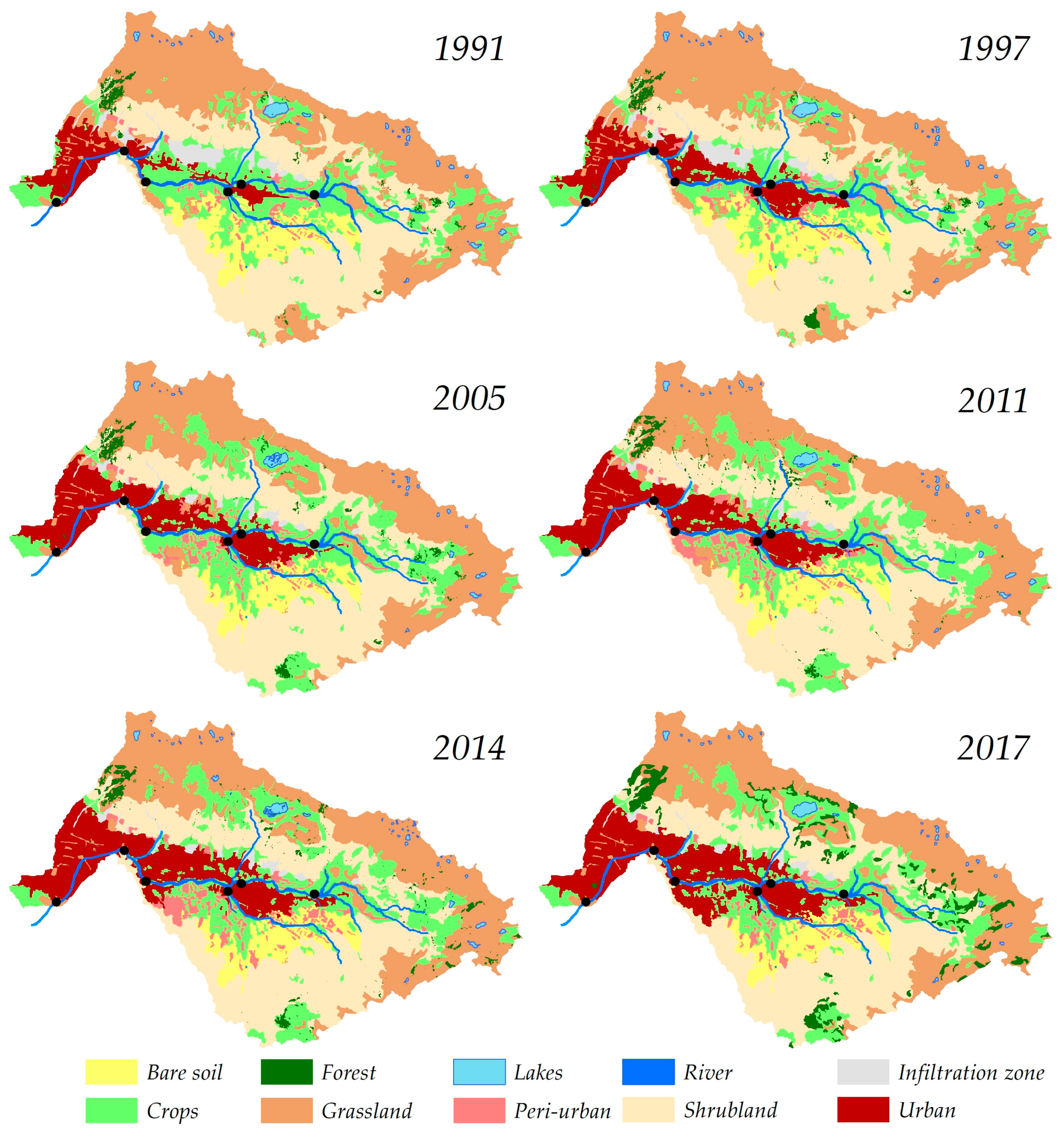
The land use classification results for each year of analysis are presented as maps in Figure 5.

Until 2011, the increasing urbanisation in the study region mainly occurred from Cochabamba city to Sacaba city and north of the Rocha River, gradually connecting the two cities. By 2014, areas south of the river between the two cities were also starting to become affected by rapid urbanisation, and by 2017 the urban areas were heavily populated and consolidated. Parallel peri-urban areas appeared as a result of transformation of land use from crops, grassland, and shrubland into urban areas.

During the study period, significant and consistent land use changes were observed, but also inconsistent changes in land use, with alternating decreases and increases in different land uses between years (

Table 5. Area (km²) and percentage of different land use classes in the Rocha River catchment in 1991 and 2017, and annual rate of land use change (%) for the periods 1991–1997, 1997–2005, 2005–2011, 2011–2014, 2014–2017, and 1991–2017.

Land Use	1991		1991–1997	1997–2005	2005–2011	2011–2014	2014–2017	1991–2017	2017
	km2	%	%	%	%	%	%	%	km2	%
Bare soil	32.6	7	0	−3	−8	3	−2	−1	23.6	5
Crops	86.9	18	−2	2	4	−9	2	0	82.3	17
Forest	5.3	1	3	12	−8	11	56	12	22.1	4
Grassland	168.8	34	0	−1	0	−1	−3	−1	134.8	28
Lakes	3.6	1	0	−4	4	−1	−2	−1	2.8	1
Peri-urban	6.9	1	4	5	−4	28	−14	2	9.9	2
River	5.8	1	0	1	0	0	0	1	6.0	1
Shrubland	139.8	29	0	0	0	0	−1	0	135.7	28
Infiltration zones	13.9	3	−1	−7	−1	3	0	−2	6.3	1
Urban	26.5	3	8	3	1	6	4	6	66.6	14

). In particular, there were inconsistent changes in the area of land used for crops and forest. The land use types occupying the greatest area throughout the study period were grassland and shrubland, whereas lakes and rivers occupied the smallest area. In 1991, shrubland and grassland occupied 29% and 34% of the catchment area, respectively; crops 18%, bare soil 7%, urban areas and (water) infiltration zones at 3% each; and peri-urban area, forest, river, and lakes at 1% each. At the end of the study period (2017), shrubland and grassland occupied 28% each; crops 17%; bare soil 5%; urban areas 14%; forest 4%; peri-urban areas 2%; and water infiltration zones, rivers, and lakes at 1% each.

In terms of annual land use change over the entire period 1991 to 2017, forest (12%), urban (6%), and peri-urban (2%) showed the highest rates of increase (Table 5). A decreasing annual rate was observed for some other land use classes, for instance, infiltration zones (−2%) and bare soil (−1%). The other land use types remained stable, with less than 1% annual change rate during the study period.

Among the land use types, forest displayed the largest annual increase in the period 2014–2017, urban in 1991–1997, and peri-urban in 2011–2014. As regards decreases in area, infiltration zones showed the largest annual decrease in 1997–2005, bare soil in 2005–2011, and crops in 2011–2014.

3.2. Water Quality and Water Flow

The data collected from former studies (1991 to 2014) and data sampled in 2017 are presented in

Table 6. Dataset (averages per year and station) collected in former studies (1991 to 2014) and the current study (2017): dissolved oxygen (DO), faecal coliforms (FC: colony-forming units (CFU)), pH, biological oxygen demand (BOD), chemical oxygen demand (COD), nitrates (NO₃), phosphates (PO₄), delta temperature, turbidity, and total solids (TS).

Year	Month	Station	n	DO	FC	pH	BOD	COD	NO3	PO4	Delta	Turbidity	TS
				% Sat.	CFU/mL		mgO2/L	mgO2/L	mg/L	mg/L	Tem. °C	NTU	mg/L
1991	May	Station 1	1	42	2.3 × 105	7.6	36.0	140.0	6.52	0.07	2.0	72	512.0
1991		Station 2	1	60	2.3 × 106	8.2	24.3	63.7	0.14	0.03	3.0	138	1512.0
1991		Station 3	1	50	2.4 × 104	7.5	3.7	56.0	4.50	0.07	4.0	90	860.0
1991		Station 4	1	95	1.4 × 104	8.6	1.8	1.9	0.04	0.09	5.0	25	45.0
1991		Station 5	1	98	2.9 × 105	7.8	1.3	1.5	0.06	0.08	9.0	10	48.7
1991		Station 6	1	90	9.3 × 104	8.2	0.8	1.2	0.03	0.05	10.0	8	47.0
1997	May and June	Station 1	3	38	9.5 × 102	7.8	36.7	220.0	8.40	0.03	0.4	19	672.0
1997		Station 2	3	16	4.3 × 106	7.4	23.0	56.0	8.54	12.75	7.7	110	966.0
1997		Station 3	3	68	7.2 × 104	7.2	24.0	32.2	0.78	0.31	2.3	450	880.0
1997		Station 4	3	6	4.0 × 104	8.1	0.4	5.0	0.16	0.23	1.4	88	96.0
1997		Station 5	3	78	6.0 × 101	6.0	1.1	1.9	0.47	0.25	10.6	32	108.1
1997		Station 6	3	59	1.6 × 103	6.9	0.4	0.9	0.07	0.09	0.6	13	37.9
2005	October	Station 1	2	42	3.1 × 106	8.0	70.5	15.9	2.21	29.79	2.0	157	522.4
2005		Station 2	1	18	3.5 × 106	8.3	61.1	13.4	0.03	22.99	2.5	130	430.3
2005		Station 3	3	38	2.8 × 106	7.0	29.0	19.7	0.81	0.18	3.5	24	80.5
2005		Station 4	1	5	2.5 × 107	8.6	2.6	4.0	4.50	1.89	4.0	92	305.0
2005		Station 5	2	6	7.4 × 101	7.6	7.2	2.9	0.07	0.26	8.0	3	8.4
2005		Station 6	2	110	1.0 × 101	8.9	1.7	5.3	0.07	0.01	13.0	92	306.0
2011	September and October	Station 1	3	12	2.5 × 106	7.6	60.8	129.0	15.52	14.25	6.0	352	992.4
2011		Station 2	3	42	3.0 × 105	7.7	164.0	209.0	0.20	30.44	0.6	100	328.0
2011		Station 3	2	21	4.0 × 106	7.9	14.0	48.0	0.33	70.26	0.7	171	433.0
2011		Station 4	1	42	5.2 × 104	9.0	2.4	89.0	0.70	9.60	3.9	66	932.0
2011		Station 5	1	28	2.0 × 102	7.6	10.0	12.0	0.18	1.78	4.7	45	79.0
2011		Station 6	1	67	2.5 × 101	8.2	1.6	2.0	0.03	0.12	12.1	4	335.0
2014	September	Station 1	1	5	8.7 × 106	7.2	214.0	342.8	15.42	35.44	5.0	115	1530.0
2014		Station 2	2	3	6.3 × 104	7.9	389.8	416.9	19.87	37.19	5.3	114	1062.0
2014		Station 3	3	3	5.4 × 104	7.5	34.4	284.2	16.39	34.53	4.7	214	1215.0
2014		Station 4	1	8	3.6 × 104	7.4	24.3	18.6	4.03	15.05	−3.8	170	676.0
2014		Station 5	2	12	1.2 × 102	8.2	21.8	12.0	2.33	10.22	1.3	95	533.0
2014		Station 6	1	90	9.4 × 101	8.3	8.9	8.7	5.85	0.01	−6.5	23	312.0
2017	June and August	Station 1	2	4	5.4 × 105	8.0	239.9	532.3	4.26	27.87	7.9	481	765.0
2017		Station 2	2	12	3.1 × 105	7.9	291.8	557.1	19.41	36.86	6.8	350	1020.0
2017		Station 3	2	3	5.0 × 107	7.1	29.0	520.0	9.36	12.80	6.4	340	743.0
2017		Station 4	2	12	2.0 × 105	7.8	37.4	40.0	12.54	33.36	1.9	260	969.0
2017		Station 5	2	18	5.6 × 105	7.8	32.0	35.0	7.75	2.98	2.9	80	2448.0
2017		Station 6	2	18	5.0 × 102	7.6	1.9	8.0	1.21	0.17	1.3	57	646.0

. The sampling years and months are related to the corresponding stations, distributed in the catchment (Figure 4). These are the values used for calculation of NSF-WQI and IPI (i.e., averages for each year/station). The complete dataset with individual sample values can be found in the Supplementary Materials of this paper. An overview of the water quality parameters measured and their summary statistics for the study period (1991–2017) are presented in

Table 7. Range and mean value of different water quality parameters at measuring stations 1–6, including their corresponding upstream sampling sites: dissolved oxygen (DO), faecal coliforms (FC: colony-forming units (CFU)), pH, biological oxygen demand (BOD), chemical oxygen demand (COD), nitrates (NO₃), phosphates (PO₄), delta temperature, turbidity, and total solids (TS).

Station		DO% Sat.	FC CFU/mL	pH	BOD mgO2/L	COD mgO2/L	NO3 mg/L	PO4 mg/L	Delta Temp. °C	Turbidity NTU	TS mg/L
1	Min	4.0	9.5 × 102	7.2	36.0	15.9	2.2	0.1	0.4	19.0	512.0
	Mean	23.8	2.5 × 106	7.7	109.7	230.0	7.1	12.9	3.9	199.3	832.3
	Max	42.0	8.7 × 106	8.0	239.9	532.3	15.5	29.8	7.9	481.0	1530.0
2	Min	3.0	6.3 × 104	7.4	23.0	13.4	0.1	0.1	0.6	100.0	328.0
	Mean	25.2	1.8 × 106	7.9	159.0	219.4	8.1	23.4	4.3	157.0	886.4
	Max	60.0	4.3 × 106	8.3	389.9	557.1	19.9	37.2	7.7	350.0	1512.0
3	Min	3.0	2.4 × 104	7.0	3.7	19.7	0.3	0.1	0.7	24.0	80.5
	Mean	30.5	9.5 × 106	7.4	22.4	160.0	5.4	19.7	3.6	214.8	701.9
	Max	68.0	5.0 × 107	7.9	34.4	520.0	16.4	70.3	6.4	450.0	1215.0
4	Min	5.0	1.4 × 104	7.4	0.4	1.9	0.1	0.1	−3.8	25.0	45.0
	Mean	28.0	5.1 × 106	8.3	11.5	26.4	3.7	10.1	2.1	116.8	503.8
	Max	95.0	2.5 × 107	9.0	37.4	89.0	12.5	33.4	5.0	260.0	969.0
5	Min	6.0	6.0 × 101	6.0	1.1	1.5	0.1	0.1	1.3	3.0	8.4
	Mean	40.0	1.4 × 105	7.5	12.2	10.9	1.8	2.6	6.1	44.2	537.5
	Max	98.0	5.6 × 105	8.2	32.0	35.0	7.8	10.2	10.6	95.0	2448.0
6	Min	18.0	1.0 × 101	6.9	0.4	0.9	0.1	0.1	−6.5	4.0	37.9
	Mean	72.3	1.6 × 104	8.0	2.6	4.4	1.2	0.1	5.1	32.8	280.7
	Max	110.0	9.3 × 104	8.9	8.9	8.7	5.8	0.2	13.0	92.0	646.0

.

At all stations except station 6, maximum and average values exceeded maximum parameter limits set by Bolivian laws and regulations. The water quality parameters that changed most negatively over the study period were COD, BOD, NO₃, PO₄, and turbidity. Other parameters such as TS also showed a negative change over the period but, contrary to expectations, no major change was found for DO. Moreover, FC, pH, and delta temperature showed no clear changes.

The overall pattern of distribution of the water quality parameters was assessed by box plot interquartile range and quartiles focused on values outside the 95% confidence limits (outliers). In general, some outliers were observed for all parameters except DO. Outliers above upper confidence limit occurred for BOD and COD, both with 14% of values above upper confidence limit, faecal coliforms (8%), and turbidity (6%). The presence of faecal pollution and domestic and industrial wastes (mainly of organic origin) could be the main causes of these high concentrations. Other parameters such as NO₃, PO₄, and TS each had 3% of values above the upper confidence limit, whereas pH and delta temperature had 3% of values below the lower confidence limit.

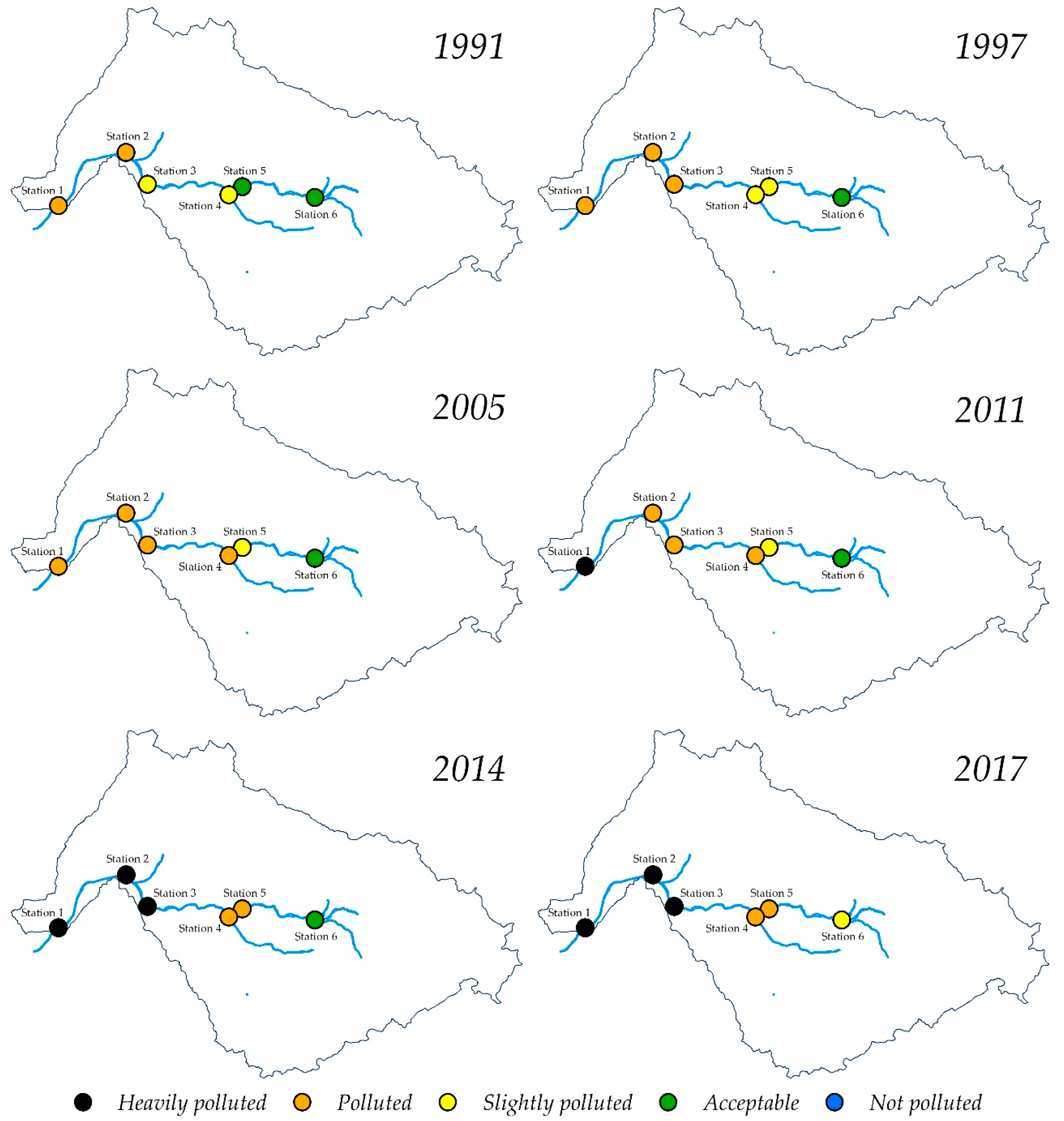
The spatial distribution of NSF-WQI values and their variation over time are presented in Figure 6 and those of IPI values in Figure 7. More detailed information on NSF-WQI quality rating and index values (calculated by means of rating equations/curves given in Ott [51] and Equation 2) and IPI quality rating and index values (calculated by means of equations in Table 3 and Equation 3) can be found in the Supplementary Materials of this paper. As can be seen in Figure 6 and Figure 7, river water quality showed a clear negative trend with time at all six measuring stations. According to both indices, water quality was relatively good in the upper part of the catchment (stations 4–6) in 1991–1997, but by 2005 the water had become more polluted. Moreover, it can also be generally seen that from 1991 to 2017 there was a decreasing trend in NSF-WQI values and an increasing trend in IPI over time, that is, a decline in water quality according to both indices at the six measuring stations (Figure 6 and Figure 7).

Statistical analyses of patterns of variations in the long-term water quality indices over time (

Table 8. Values of Mann–Kendall’s tau and Theil–Sen slope obtained for the National Sanitation Foundation-Water Quality Index (NSF-WQI) and Prati’s Implicit Index of Pollution (IPI) at measuring stations 1–6, 1991–2017.

NSF-WQI	Station
	1	2	3	4	5	6
Mann–Kendall´s tau	−0.733	−0.467	−0.600	−0.867	−1	−0.467
p-value	0.060	0.259	0.133	0.024 *	0.008 *	0.259
Theil–Sen’s slope	−3.63	−4.60	−6.02	−7.53	−7.70	−2.10
IPI	1	2	3	4	5	6
Mann–Kendall´s Tau	1	0.867	0.867	0.966	0.734	0.414
p-value	0.008 *	0.024 *	0.024 *	0.013 *	0.060	0.339
Theil–Sen’s slope	8.88	14.47	3.62	1.70	1.52	0.30

* Significant at p < 0.05.

) showed significant (p < 0.05) decreasing trends at stations 4 and 5 for NSF-WQI (negative Theil–Sen slope values) and significant (p < 0.05) increasing trends at stations 1, 2, 3, 4, and 5 for IPI (positive Theil–Sen slope values) during the study period (1991–2017). These relationships confirm the indications in Figure 6 and Figure 7 that Rocha River water has become increasingly polluted over time.

Water flow or discharge corresponding to the six stations (former and current studies), measured during the dry season (May to October) was within the ranges of 0.02–0.60, 0.03–0.10, 0.01–0.90, 0.01–0.50, 0.01–0.30, and 0.01–0.31 m⁻³ s⁻¹ for stations 1–6, respectively. Water flow volumes in the region are generally low in the dry season. At station 1 (catchment outlet), the river receives discharges of sewage water and effluent from industries [55]. Farther upstream, at station 2, the water flow is lower, mainly due to constant water extraction for nearby irrigation schemes. At station 3, upstream water flow is also used for irrigation and the river receives domestic sewage, effluent from small industries, and discharges from other illegal drains. Station 4 is located on the southern branch of the river that collects sewage water from Sacaba city. It also receives a considerable amount of effluent from the main slaughterhouse south of Sacaba city. The surrounding area comprises mostly peri-urban and agricultural land, but there was no evidence of irrigation using water from the southern branch during the study period, with farming on this land being dominated by rain-fed crops. At station 5, water flow is influenced by extraction for irrigation, but mainly for vegetated areas in Sacaba city, and for some agricultural fields and other domestic usage [56]. Water flow at station 6 is reduced due to the presence of small natural creeks, the water in which is used for irrigation. It is important to mention that in the past 20 years, water reservoirs or tanks of water for human consumption have been constructed at many households. It is estimated that 15% of the water supply in the catchment was captured in this way in 2012 [21].

3.3. Water Quality and Land Uses

A Spearman’s rho rank correlation analysis was carried out between each of the two water quality indices and the percentage of different land uses present in the adjacent upstream sub-catchments (

Table 9. Correlation coefficients (Spearman’s rho) for each of the water quality indices (NSF-WQI and IPI) and the corresponding land use (% of sub-catchment area) for stations 1–6, 1991–2017.

Land Use Type		NSF-WQI Values at Station:						IPI Values at Station:
		1	2	3	4	5	6	1	2	3	4	5	6
Bare soil	rho	–	–	0.64	0.41	0.71	−0.10	–	–	−0.78	−0.83	−0.54	0.71
	p-value	–	–	0.173	0.414	0.136	0.842	–	–	0.065	0.042 *	0.297	0.136
Crops	rho	0.76	0.66	0.14	0.31	−0.43	0.48	−0.91	−0.31	−0.08	−0.14	0.43	−0.43
	p-value	0.076	0.175	0.803	0.564	0.419	0.355	0.011 *	0.563	0.919	0.802	0.419	0.419
Forest	rho	−0.06	−0.06	−0.60	0.06	−0.83	−0.41	0.12	0.46	0.48	0.46	0.88	−0.83
	p-value	0.913	0.913	0.242	0.913	0.058	0.424	0.827	0.354	0.355	0.354	0.034 *	0.058
Grassland	rho	0.77	0.35	0.84	0.79	0.77	0.23	−0.94	−0.64	−0.84	−0.91	−0.94	0.77
	p-value	0.103	0.499	0.030 *	0.059	0.102	0.658	0.017 *	0.173	0.034 *	0.011 *	0.017 *	0.102
Peri–urban	rho	0.09	0.38	−0.88	−0.09	−0.43	−0.74	−0.27	−0.79	0.76	0.14	0.43	−0.43
	p-value	0.864	0.454	0.020 *	0.919	0.419	0.095	0.600	0.059	0.080	0.802	0.419	0.419
Urban	rho	−0.88	−0.71	−0.89	−0.77	−0.98	0.62	0.85	0.94	0.98	0.94	0.89	−0.98
	p-value	0.033 *	0.136	0.015 *	0.103	0.002 *	0.191	0.002 *	0.017 *	0.000 **	0.017 *	0.033 *	0.002 *
Shrubland	rho	−0.62	−0.64	−0.03	−0.15	0.69	0.35	0.62	0.93	0.18	−0.28	−0.69	0.69
	p-value	0.191	0.173	0.961	0.770	0.123	0.492	0.191	0.007 *	0.737	0.584	0.128	0.123
Infiltration zone	rho	0.44	0.09	–	0.11	0.58	−0.17	−0.53	−0.50	–	−0.46	−0.52	0.58
	p-value	0.380	0.868	–	0.827	0.231	0.748	0.279	0.312	–	0.354	0.294	0.231

** Significant at p < 0.001; * significant at p < 0.05.

).

There was a significant (p < 0.05) negative relationship between NSF-WQI and urban area at stations 1, 3, and 5. At station 3, a significant (p < 0.05) negative relationship was found between NSF-WQI and peri-urban area, and a significant (p < 0.05) positive relationship between NSF-WQI and grassland. There was a highly significant (p < 0.001) positive relationship between IPI and urban area at station 3 and a significant (p < 0.05) positive relationship at stations 1, 2, 4, 5, and 6. There was a significant (p < 0.05) negative relationship between IPI and crops at station 1, between IPI and shrubland at station 2, between IPI and bare soil at station 4, and between IPI and grassland at stations 1, 3, 4, and 5.

The relationships between the NSF-WQI/IPI values and the percentage of different land use types in the whole catchment area are shown in

Table 10. Statistical analysis (Spearman’s rho) of each of the water quality indices (NSF-WQI and IPI) and the corresponding land use (% of total area) in the whole catchment, 1991–2017.

Land Use Type	NSF-WQI		IPI
	rho	p-value	rho	p-value
Bare soil	0.24	0.153	−0.53	0.000 **
Crops	0.39	0.016 *	−0.44	0.006 *
Forest	0.05	0.974	0.16	0.343
Grassland	0.25	0.133	−0.11	0.533
Peri-urban	−0.27	0.111	0.04	0.807
Urban	−0.72	0.000 **	0.89	0.000 **
Shrubland	0.18	0.283	−0.49	0.001 *
Infiltration zone	−0.22	0.195	−0.36	0.031 *

** Significant at p < 0.001, * significant at p < 0.05.

.

A highly significant (p < 0.001) negative relationship was found between NSF-WQI and urban area and between IPI and bare soil. A highly significant (p < 0.001) positive relationship was found between IPI and urban area. Furthermore, significant (p < 0.05) negative relationships were observed between IPI and crops, between IPI and shrubland, and between IPI and infiltration zone. Finally, a significant (p < 0.05) positive relationship was observed between NSF-WQI and crops.

Regression analysis (simple and monotonic) was performed for the significant relationships found between land use type and either WQI. The results revealed fairly small but significant R² values for all combinations except that between IPI and bare soil and that between IPI and infiltration zone.

Some similarities and differences can be observed in comparing Table 9 (by station/sub-catchment) and Table 10 (whole catchment). For example, urban land use type was significantly related to NSF-WQI and IPI at different stations (stations 1, 3, and 5 for NSF-WQI and stations 1–6 for IPI) (Table 9) and in the whole catchment (Table 10). NSF-WQI was significantly related to crops at catchment level, but not at station level. NSF-WQI was significantly related to grassland and peri-urban at station 3, but not at catchment level. IPI was not related to grassland at catchment level, but was significantly related at stations 1, 3, 4, and 5. IPI was also significantly related at catchment level to bare soil, crops, and shrubland. At station level, IPI was significantly related to bare soil at station 4, to crops at station 1, and to shrubland at station 2. IPI was significantly related to forest at station 5, but not at catchment level.

4. Discussion

When planning future water management measures, it is essential to have knowledge about how former land use has affected the current water status, both regarding water availability and water quality. In order to perform satisfactory assessments, it is crucial to have reliable input data. The frequent lack of measured data creates a need for a simple and fast way of describing potential driver(s) associated with changes in water flow induced by rainfall and in selected water quality indices that accurately describe changes in water quality. In this study, land use information on the Rocha River catchment for 1991, 1997, 2005, 2011, 2014, and 2017 was used to examine the association between land use and surface water quality. Historical data from former studies (1991–2014) were combined with current data (2017), covering a total study period of 26 years.

A clear increasing trend in mean annual temperature was observed in the study period 1991–2017, whereas no clear trend in annual total precipitation was identified (Figure 3). Furthermore, the period 1991–2017 had higher total mean annual temperature than the period 1964–1990 (Figure 2). It is generally claimed that climate change has caused a reduction in streamflow in the Rocha River and in other similar catchments in South America [57]. According to the climate and land use observations obtained in the present study, this reduction may be caused by increased evapotranspiration and increased water use for irrigation and for industrial and domestic purposes.

The annual land use change rate calculations provided a synoptic and quantitative view of the land use types and spatial and temporal changes in land use in the study area (Figure 5, Table 5). The results revealed that during the period 1991–2017, forest, urban, and peri-urban land uses in the study catchment increased at the expense of water infiltration zones and bare land, with the latter land use showing the greatest decrease. Furthermore, there were changes between years in the area of land used for crops. Between 2014 and 2017 there was an increase, mainly related to a government incentive that provided subsidies for fertilisers and seeds [38]. The changes in forest over time revealed initial effects of various afforestation programmes such as PROFOR [58], funded by local and national institutions and external foundations. For example, Nature Fund [59] and the Fontana foundation [60], among others, have been involved in integrated watershed management of Tunari National Park, in the northern part of the catchment. To summarise, the increasing process of urban expansion and population growth over time have converted adjacent land use types into peri-urban or urban use, whereas at the same time the forested area in the catchment has increased. To complement the results obtained in the present study, modified classes (land use types) with clear temporal and spectral properties could be defined and oriented to specific goals (increase, decrease, or no change in area occupied by the respective land use type).

On reviewing secondary sources of data and information, we found that most of the values reported in former studies in the catchment were obtained by sampling or measuring water quality and flow parameters, rather than analyses including modelling and/or multivariate statistics to determine the relationship between land use and water quality. As background, it is important to note that the sampling for each campaign between 1991 and 2014 was based on specific needs and performed using standard methods and well-known procedures in field work at the time of each study, taking into account pollution processes and mandatory requirements from authorities.

In the present study, only the dry season (May to October) was assessed. During this period, the relative water flow is generally much lower and contributes to a higher concentration of pollutants. This may be one of the reasons why a generally polluted (slightly to heavily) response was found at all stations for both WQIs by 2017. Any differences arising between the NSF-WQI and IPI values (Figure 6 and Figure 7) were caused by the different numbers of parameters included in NSF-WQI (nine parameters) and IPI (four parameters), the presence of chemical oxygen demand in IPI (lacking in NFS-WQI), and its organic pollution orientation [17], as well as the weighting values for parameters used in NSF-WQI. For instance, the greater gradient between station 6 and 1 for IPI (not polluted to very polluted) (Figure 7), as compared with NSF-WQI (acceptable to polluted) (Figure 6), the first years (1991, 1997, and 2005) may be explained by increasing values of chemical oxygen demand (2.5 to 125.3 mgO₂/L), which is not included in NSF-WQI. Furthermore, the weights assigned to biological oxygen demand and nitrate (see Table 2) could attenuate the potential pollution effect. Parameter selection is thus an important issue to consider when planning to assess water quality by a selected WQI. Reducing the number of parameters included in a WQI can result in more variation in the values obtained, as in the present study.

The NSF-WQI approach focuses on the physicochemical and biological quality of water, whereas the IPI approach focuses on organic pollution. As reported by numerous authors [61,62,63,64,65], both these indices are very sensitive to the sampling period, that is, whether it is rainy or dry, and its effect on dilution or concentration of the parameters. Owing to the effect of air temperature on water quality parameters by influencing physical, biological, and chemical processes, time of sampling is important. According to de Souza et al. [66], water quality parameters in the study region are acceptable to bad in the dry season and predominantly good in the wet season. In the present study, only the dry season was assessed due to the water quality decline during that season and to lack of data on the wet season, as noted in local reports [14,15,16]. Maximum concentrations of pollutants could thus be found in the dry season because of reduced precipitation and water flow volumes, therefore impeding the effects of natural dilution and self-purification capacity of the river [67].

The WQIs tested were confirmed to be useful tools for assessing spatial and temporal changes and for classifying river water quality. These indices provide quantifiable values of the degree of pollution, and therefore a combined summary of information on several parameters in a single value. This allows the general status of water to be evaluated, classified, and compared (bringing data from several studies into one database to track changes) in different time periods. The utility of WQIs was also recognised by Giri and Qui [4], for example, who concluded that these indices provide an overall picture of watershed pollution generation characteristics, and by Kannel et al. [34] in evaluating spatial and seasonal changes in the water quality in a river basin in Nepal for 5 years. The latter analysis showed that water quality was lowest in winter, was related to urban areas, and decreased from 1999 to 2003. These results are similar to the findings reported in the present study. In a study in a Chilean river basin, Debels et al. [35] found good general water quality throughout the year, but severely deteriorated conditions during summer at stations downstream of an urban wastewater discharge.

The two WQIs applied in the present study showed significant temporal and, to a certain degree, spatial variability from upstream all the way down to the outlet of the catchment (Figure 6 and Figure 7, Table 7, Table 8 and Table 9). Stations 1, 2, and 5 were related to urban areas; 3 and 4 to peri-urban areas; and station 6 to grassland and crops, and in the last years to peri-urban areas. The increasing pollutant load gradient from upstream (station 6) to downstream at the catchment outlet, with clear increments in chemical and biological oxygen demand values, is most probably related to sewage water. On the other hand, the low dissolved oxygen values found are related to organic matter abundance.

The temporal (1991 to 2017) behaviour was also consistent throughout the period. In the 1990s, low population and limited commercial activities characterised the study area. However, agriculture and livestock were already established. By the early 2000s, some industries related to tanneries, construction work, food and beverage production, and paper production had been established in the study catchment, affecting stations 1, 2, and 3. Between 2005 and 2011, a slaughterhouse with no system for water treatment was built downstream from station 4. As a consequence, a high organic load began to be discharged directly into the river, affecting stations 2 and 3. At the same time, the population increased and the Sacaba region started to become a dormitory area for people working mainly in Cochabamba city. From this period onward, agriculture started to receive government subsides, which increased agricultural areas and production. In 2014, a small water treatment plant for domestic wastewater was built a short distance upstream of station 2, but the capacity was limited to serving 350 households. During that time, policies regarding land occupation were established by local authorities, which led to more people selling and buying land. In 2017, a medium-sized wastewater plant was installed downstream of station 3, but it is currently only working at between 10% and 20% of its capacity. Population is concentrated in urban areas (stations 1, 2, and 5), which are expanding through peri-urban areas, leading to increasing loads at stations 3 and 4 and, to a smaller extent, at station 6. No effective treatment is present for agricultural water runoff, domestic sewage water, and industrial spills.

The variations in NSF-WQI and IPI values along river sections are thus related mainly to illegal or untreated domestic sewage water and small industrial spills and solid wastes, most of which were verified during fieldwork in 2017. A similar situation is reported by Shi et al. [68] in Melbourne, Australia, where water quality decreases are likely caused by phosphates in detergents, construction waste, illegal wastewater discharge, and industrial spills. In a study in Campo Grande, Brazil, de Souza et al. [66] found that land use and occupation, increasing population density, and lack of sanitation are related to water pollution. Wastewater discharge and nutrient runoff were found by Carstens et al. [69] to ultimately lead to impaired water quality in Louisiana, USA.

The NSF-WQI and IPI values obtained in the present study revealed decreasing water quality with increasing urban area in the catchment. They also indicated higher water quality with greater area of bare soil, crops, shrubland, and infiltration zones. Positive relationships between NSF-WQI/IPI and urban area were also observed at station level (including their respective upstream sites); for example, urban area was a determinant for NSF-WQI at stations 1, 3, and 5, and for IPI at stations 1–6 (Table 9). Natural land use types (bare soil, grassland, shrubland) also played an important role within sub-catchments at station level, as did crops and forest, and all were associated with improving water quality values. Thus, the stations, and their related sub-catchment, were a source of variation in WQI values, as they varied in land use type proportion and change during the study period. At station 3 in particular, urban area and, to a certain extent, peri-urban area played a significant role in the degradation in water quality over the study period by giving rise to discharge from septic tanks and leaking sewers directly into the riverbed. Hence, urban and peri-urban land use types can be considered the main determining factors for surface water quality in the Rocha River catchment. Using simple regression, Chu et al. [6] found that water quality in Taiwan is related to land use and concluded that understanding this relationship is useful for watershed management and pollution prevention plans. Similar findings have been reported by Haidary et al. [9] in a study in Japan, which are in line with the finding in this study.

The results from the present study, showing declining water quality following urban and economic growth, are in line with previous findings that urbanisation has negative impacts on the environment [69]. One of the consequences of this is that areas that are not yet exploited may become inappropriate waste disposal areas, and their pollutants reach rivers due to the lack of adequate public policies for urban water management. The results presented here thus provide a baseline for future monitoring of the Rocha River. The results also indicate that water pollution prevention strategies, such as an initial stakeholder analysis related to pollution and contamination, an effective continuous monitoring control programme, pollution mitigation and remediation in critical areas, and restoration of water quality to adequate levels, should be implemented for proper water quality management along the Rocha River.

For effective water quality management, it is recommended that studies are made on classification of freshwater ecosystems; clear and targeted selection of pollution parameters; non-point pollution source evaluation on runoff pollutant transport; risk analysis on the effects of the pollution on human, environmental, and ecosystem health; and an estimate of the cost of intervention.

5. Conclusions

Changes in land use in the study area over time were characterised by an important increase in forest, urban, and peri-urban areas, and a decrease in water infiltration zones, bare soil, grassland, and shrubland areas.

Over the study period (dry season 1991–2017), there was a clear trend in NSF-WQI and IPI values, indicating that surface water quality in the study area had deteriorated dramatically. In particular, the values indicated that water quality declines with increasing proportion of urban area and improves with increasing proportion of cropped area. The IPI values also indicated higher water quality with higher proportions of bare soil, shrubland, and infiltration zones within the catchment.

Due to the simplicity and practicality of the WQI approach presented here and the acceptable level of accuracy achieved, both NSF-WQI and IPI can be recommended for use in assessment of surface water quality in other study areas. The values of both WQIs can be used to define environmental policies, crop production systems, and land use planning programmes.

References

- Sajikumar, N.; Remya, R. Impact of land cover and land use change on runoff characteristics. J. Environ. Manag. 2015, 161, 460–468. [Google Scholar] [CrossRef] [PubMed]
- Miller, J.; Kim, H.; Kjeldsen, T.; Packman, J.; Grebby, S.; Dearden, R. Assessing the impact of urbanization on storm runoff in a peri-urban catchment using historical change in impervious cover. J. Hydrol. 2014, 515, 59–70. [Google Scholar] [CrossRef] [Green Version]
- Nie, W.; Yuan, Y.; Kepner, W.; Nash, M.; Jackson, M.; Erickson, C. Assessing impacts of landuse and landcover changes on hydrology for the upper San Pedro watershed. J. Hydrol. 2011, 407, 105–114. [Google Scholar] [CrossRef]
- Giri, S.; Qiu, Z. Understanding the relationship of land uses and water quality in Twenty First Century: A review. J. Environ. Manag. 2016, 173, 41–48. [Google Scholar] [CrossRef] [Green Version]
- Foley, J.; DeFries, R.; Asner, G.; Barford, C.; Bonan, G.; Carpenter, S.; Chapin, F.; Coe, M.; Daily, G.; Gibbs, H.; et al. Global consequences of land use. Science 2005, 309, 570–574. [Google Scholar] [CrossRef]
- Chu, H.; Liu, C.; Wang, C. Identifying the relationships between water quality and land cover changes in the Tseng-Wen reservoir watershed of Taiwan. Int. J. Environ. Res. Public Health 2013, 10, 478–489. [Google Scholar] [CrossRef]
- Kamarinas, I.; Julian, J.; Hughes, A.; Owsley, B.; De Beurs, K. Nonlinear changes in land cover and sediment runoff in a New Zealand catchment dominated by plantation forestry and livestock grazing. Water 2016, 8, 436. [Google Scholar] [CrossRef]
- Li, S.; Gu, S.; Liu, W.; Han, H.; Zhang, Q. Water quality in relation to land use and land cover in the upper Han River Basin, China. Catena 2008, 75, 216–222. [Google Scholar] [CrossRef]
- Haidary, A.; Amiri, B.; Adamowski, J.; Fohrer, N.; Nakane, K. Assessing the impacts of four land use types on the water quality of wetlands in Japan. Water Resour. Manag. 2013, 27, 2217–2229. [Google Scholar] [CrossRef]
- Tong, S.; Chen, W. Modeling the relationship between land use and surface water quality. J. Environ. Manag. 2002, 66, 377–393. [Google Scholar] [CrossRef]
- Ahearn, D.; Sheibley, R.; Dahlgren, R.; Anderson, M.; Johnson, J.; Tate, K. Land use and land cover influence on water quality in the last free-flowing river draining the western Sierra Nevada, California. J. Hydrol. 2005, 313, 234–247. [Google Scholar] [CrossRef]
- Tu, J. Spatially varying relationships between land use and water quality across an urbanization gradient explored by geographically weighted regression. Appl. Geogr. 2011, 31, 376–392. [Google Scholar] [CrossRef]
- Chen, Q.; Mei, K.; Dahlgren, R.; Wang, T.; Gong, J.; Zhang, M. Impacts of land use and population density on seasonal surface water quality using a modified geographically weighted regression. Sci. Total Environ. 2016, 572, 450–466. [Google Scholar] [CrossRef] [PubMed] [Green Version]
- Contraloria General del Estado. Informe de Auditoría Sobre el Desempeño Ambiental Respecto de los Impactos Negativos Generados en el Río Rocha; K2/AP06/M11; Gestión de Evaluación Ambiental: Cochabamba, Bolivia, 2011; p. 320.
- Gobierno Autónomo Municipal de Sacaba. Propuesta de Clasificación del río Rocha en Función a su Aptitud de Uso; Dirección de Madre Tierra y Medio Ambiente: Cochabamba, Bolivia, 2014; p. 167.
- Prefecture of the Departament of Cochabamba. Estudios Básicos de la Cuenca del Río Rocha; Prefecture of the Departament of Cochabamba: Cochabamba, Bolivia, 2005; p. 314.
- Romero, A.; Van Damme, P.; Goitia, E. Contaminación orgánica en el río Rocha (Cochabamba, Bolivia). Revista Boliviana de Ecología y Conservación Ambiental 1998, 8, 37–47. [Google Scholar]
- Coronado, O.; Moscoso, Ó.; Claros, L. Estudio de Viabilidad Cochabamba, Bolivia; Organización Panamericana de la Salud: Lima, Perú, 2002; p. 80. [Google Scholar]
- Dost, R. Hydrologic Information Systems as a Support Tool for Water Quality Monitoring A Case Study in the Bolivian Andes; Research, International Institute for Geo-information Science and Earth Observation: Enschede, The Netherlands, 2005. [Google Scholar]
- Gobierno Autónomo Municipal de Sacaba. Prácticas de Saneamiento Ambiental Sostenibles en la Cuenca del Río Maylanco; Consultora INAXO: Cochabmaba, Bolivia, 2011; p. 37.
- Bolivian Ministry of Environment and Water. Plan Maestro Metropolitano de Agua y Saneamiento del Área Metropolitana de Cochabamba Bolivia; Bolivian Ministry of Environment and Water: La paz, Bolivia, 2012; p. 680.
- Programa de Aguas; Programa de Hidronomia. Informe Tecnico IX, Monitoreo del Río Rocha; Universidad Mayor de San Simón: Cochabmba, Bolivia, 1992; p. 6. [Google Scholar]
- Toledo, R.; Amurrio, D. Evaluación de la calidad de las aguas del río Rocha en la jurisdicción de SEMAPA en la provincia Cercado de Cochabamba-Bolivia. Acta Nova 2006, 3, 521–542. [Google Scholar]
- Vergara, S. Indices de Calidad de agua Como Indicador De Contaminación Y Su Distribución Espacio-Temporal En El río Rocha. Magister profesional; Universidad Mayor de San Simón: Cochabamba, Bolivia, 2001. [Google Scholar]
- De La Mora-Orozco, C.; Flores-Lopez, H.; Rubio-Arias, H.; Chavez-Duran, A.; Ochoa-Rivero, J. Developing a Water Quality Index (WQI) for an irrigation dam. Int. J. Environ. Res. Public Health 2017, 14, 439. [Google Scholar] [CrossRef]
- Sutadian, A.; Muttil, N.; Yilmaz, A.; Perera, B. Development of river water quality indices—A review. Environ. Monit. Assess. 2016, 188, 58. [Google Scholar] [CrossRef]
- Horton, R. An index number system for rating water quality. J. Water Pollut. Control Fed. 1965, 37, 300–306. [Google Scholar]
- Brown, R.; McClelland, N.; Deininger, R.; Tozer, R. A Water Quality Index—Do we dare? Water Sew. Works 1970, 117, 339–343. [Google Scholar]
- Brown, R.; McClelland, N.; Deininger, R.; Landwehr, J. Validating the WQI. In Proceedings of the Paper Presented at National Meeting of American Society of Civil Engineers on Water Resources Engineering, Washington, DC, USA, 29 January–2 February 1973. [Google Scholar]
- Prati, L.; Pavanello, R.; Pesarin, F. Assessment of surface water quality by a single index of pollution. Water Res. 1971, 5, 741–751. [Google Scholar] [CrossRef]
- Lumb, A.; Sharma, T.; Bibeault, J. A Review of genesis and evolution of Water Quality Index (WQI) and some future directions. Water Qual. Expo. Health 2011, 3, 11–24. [Google Scholar] [CrossRef]
- Sener, S.; Sener, E.; Davraz, A. Evaluation of water quality using water quality index (WQI) method and GIS in Aksu River (SW-Turkey). Sci. Total Environ. 2017, 584–585, 131–144. [Google Scholar] [CrossRef] [PubMed]
- Ewaid, S.; Abed, S. Water quality index for Al-Gharraf River, southern Iraq. Egypt. J. Aquat. Res. 2017, 43, 117–122. [Google Scholar] [CrossRef]
- Kannel, P.R.; Lee, S.; Lee, Y.S.; Kanel, S.R.; Khan, S.P. Application of water quality indices and dissolved oxygen as indicators for river water classification and urban impact assessment. Environ. Monit. Assess. 2007, 132, 93–110. [Google Scholar] [CrossRef]
- Debels, P.; Figueroa, R.; Urrutia, R.; Barra, R.; Niell, X. Evaluation of water quality in the Chillan River (Central Chile) using physicochemical parameters and a modified water quality index. Environ. Monit. Assess. 2005, 110, 301–322. [Google Scholar] [CrossRef]
- Salcedo-Sánchez, E.; Hoyos, S.; Alberich, M.; Morales, M. Application of water quality index to evaluate groundwater quality (temporal and spatial variation) of an intensively exploited aquifer (Puebla valley, Mexico). Environ. Monit. Assess. 2016, 188, 573. [Google Scholar] [CrossRef]
- Instituto Nacional de Estadística. Principales Resultados del Censo Nacional de Población y Vivienda 2012; Estado Plutrinacional de Bolivia: La Paz, Bolivia, 2013; p. 56.
- Gobierno Autónomo Municipal de Sacaba. Plan Territorial de Desarrollo Integral—PTDT; Territorial, O., Ed.; Secretaria Municipal de Planificación y Desarrollo Territorial: Sacaba, Cochabamba, Bolivia, 2016; p. 294.
- Kennan, L.; Lamb, S.; Rundle, C. K-Ar Dates from the Altiplano and Cordillera-Oriental of Bolivia—Implications for cenozoic stratigraphy and tectonics. J. S. Am. Earth Sci. 1995, 8, 163–186. [Google Scholar] [CrossRef]
- Ongaro, L.; l’Oltremare, I.A.P.; Esteri, I.M.D.A. Land Evaluation of the Valley of Sacaba (Bolivia); Istituto agronomico per l’Oltremare: Firenze, Italy, 1998.
- Metternicht, G.; Fermont, A. Estimating erosion surface features by linear mixture modeling. Remote Sens. Environ. 1998, 64, 254–265. [Google Scholar] [CrossRef]
- Metternicht, G.; Gonzalez, S. FUERO: Foundations of a fuzzy exploratory model for soil erosion hazard prediction. Environ. Model. Softw. 2005, 20, 715–728. [Google Scholar] [CrossRef]
- Environmental Resources Management. Estudios Básicos de Mitigación y Adaptación al Cambio Climático, Vulnerabilidades, Huella Urbana Y Escenarios de Crecimiento Urbano Y Para La Región Metropolitana de Cochabamba; Inter-American Development Bank: Washington, DC, USA, 2013; p. 120. [Google Scholar]
- Congalton, R.; Green, K. Assessing the Accuracy of Remotely Sensed Data: Principles and Practices; CRC Press, Taylor and Francis Group: Boca Raton, FL, USA, 2008. [Google Scholar]
- Cohen, J. A Coefficient of agreement for nominal scales. Educ. Psychol. Meas. 1960, 20, 37–46. [Google Scholar] [CrossRef]
- Dirección de Madre Tierra y Medio Ambiente. Informe de Monitoreo Cuenca del Río Rocha—Sacaba; Gobierno Autónomo Municipal de Sacaba: Cochabamba, Bolivia, 2015; p. 24.
- Chilundo, M.; Kelderman, P.; Okeeffe, J. Design of a water quality monitoring network for the Limpopo River Basin in Mozambique. Phys. Chem. Earth 2008, 33, 655–665. [Google Scholar] [CrossRef] [Green Version]
- APHA; AWWA; WEF. Standard methods for the examination of water and wastewater. In Public Health Association; APHA: Washington, DC, USA, 1992; Volume 18. [Google Scholar]
- ASTM. Standards for Water and Wastewater; American Society for Testing Materials: Philadelphia, PA, USA, 1958. [Google Scholar]
- Abbasi, T.; Abbasi, S. ‘Conventional’ indices for determining fitness of waters for different uses. In Water Quality Indices; Elsevier: Amsterdam, The Netherlands, 2012; pp. 25–62. [Google Scholar] [CrossRef]
- Ott, W. Environmental Indices: Theory and Practice; Ann Arbor Science Publishers, Inc.: Ann Arbor, Michigan, USA, 1978; pp. 202–215. [Google Scholar]
- Hirsch, R.; Slack, J.; Smith, R. Techniques of trend analysis for monthly water quality data. Water Resour. Res. 1982, 18, 107–121. [Google Scholar] [CrossRef] [Green Version]
- Sheikhy, T.; Aris, A.; Sefie, A.; Keesstra, S. Detecting and predicting the impact of land use changes on groundwater quality, a case study in Northern Kelantan, Malaysia. Sci. Total Environ. 2017, 599–600, 844–853. [Google Scholar] [CrossRef] [PubMed]
- Du, X.; Huang, Z. Ecological and environmental effects of land use change in rapid urbanization: The case of hangzhou, China. Ecol. Indic. 2017, 81, 243–251. [Google Scholar] [CrossRef]
- Peredo, M.; Perez, J. Auditoria Especializada sobre el Desempeño Ambiental De Empresas Que Suministran Agua Potable A Las Ciudades de La Paz, El Alto y Cochabamba; Bachellor Project; University of San Andres: La Paz, Bolivia, 2010. [Google Scholar]
- Ayala, R.; Acosta, F.; Mooij, W.; Rejas, D.; Van Damme, P. Management of Laguna Alalay: A case study of lake restoration in Andean valleys in Bolivia. Aquat. Ecol. 2007, 41, 621–630. [Google Scholar] [CrossRef]
- Fries, A.; Rollenbeck, R.; Nauß, T.; Peters, T.; Bendix, J. Near surface air humidity in a megadiverse Andean mountain ecosystem of southern Ecuador and its regionalization. Agric. For. Meteorol. 2012, 152, 17–30. [Google Scholar] [CrossRef]
- Robledo, C.; Fischler, M.; Patiño, A. The Role of Community-Based Forest Land Rehabilitation in Building Resilience to Climate Impacts: A Case Study from the PROFOR-Afforestation Project in the Community of Khuluyo Cochabamba, Bolivia; Intercooperation Working Paper; Intercooperation: Bern, Switzerland, 2003. [Google Scholar]
- Wiese, K.; Klette, C. Save Bolivian Jungle. Available online: https://www.naturefund.de/en/about_us/our_vision/ (accessed on 20 July 2018).
- USER, S. Reforestation in Cochabamba, Bolivia. Available online: http://fontana-foundation.org/data3/index.php/en/closed-projects/reforestation-bolivia (accessed on 15 July 2018).
- Hasan, H.; Jamil, N.; Aini, N. Water quality index and sediment loading analysis in Pelus River, Perak, Malaysia. Procedia Environ. Sci. 2015, 30, 133–138. [Google Scholar] [CrossRef]
- Lai, Y.; Tu, Y.; Yang, C.; Surampalli, R.; Kao, C. Development of a water quality modeling system for river pollution index and suspended solid loading evaluation. J. Hydrol. 2013, 478, 89–101. [Google Scholar] [CrossRef]
- Ramos, M.; de Oliveira, E.; Piao, A.; Leite, D.; de Angelis, F. Water Quality Index (WQI) of Jaguari and Atibaia Rivers in the region of Paulinia, Sao Paulo, Brazil. Environ. Monit. Assess. 2016, 188, 263. [Google Scholar] [CrossRef]
- Rubio-Arias, H.; Contreras-Caraveo, M.; Quintana, R.; Saucedo-Teran, R.A.; Pinales-Munguia, A. An overall Water Quality Index (WQI) for a man-made aquatic reservoir in Mexico. Int. J. Environ. Res. Public Health 2012, 9, 1687–1698. [Google Scholar] [CrossRef]
- Wang, Q.; Wu, X.; Zhao, B.; Qin, J.; Peng, T. Combined multivariate statistical techniques, Water Pollution Index (WPI) and Daniel Trend Test methods to evaluate temporal and spatial variations and trends of water quality at Shanchong River in the Northwest Basin of Lake Fuxian, China. PLoS ONE 2015, 10, e0118590. [Google Scholar] [CrossRef] [PubMed]
- de Souza, M.; Cavalheri, P.; de Oliveira, M.; Magalhães, F. A multivariate statistical approach to the integration of different land-uses, seasons, and water quality as water resources management tool. Environ. Monit. Assess. 2019, 191, 539. [Google Scholar] [CrossRef] [PubMed]
- Bora, M.; Goswami, D. Water quality assessment in terms of water quality index (WQI): Case study of the Kolong River, Assam, India. Appl. Water Sci. 2016, 7, 3125–3135. [Google Scholar] [CrossRef]
- Shi, B.; Bach, P.; Lintern, A.; Zhang, K.; Coleman, R.A.; Metzeling, L.; McCarthy, D.T.; Deletic, A. Understanding spatiotemporal variability of in-stream water quality in urban environments—A case study of Melbourne, Australia. J. Environ. Manag. 2019, 246, 203–213. [Google Scholar] [CrossRef] [PubMed]
- Carstens, D.; Amer, R. Spatio-temporal analysis of urban changes and surface water quality. J. Hydrol. 2019, 569, 720–734. [Google Scholar] [CrossRef]
Figure 1.
Location and topography of the Rocha River catchment.
Figure 2.
Median and variation in annual values of (a) mean temperature and (b) total rainfall at the outlet of the Rocha River catchment in two 26 year periods (1964–1990, 1991–2017).
Figure 3.
Total rainfall (blue bars) and mean temperature (dots between orange lines and fitted least-square line for the total period) in the Rocha River catchment in each year between 1991 and 2017.
Figure 4.
Map of the study area showing sub-catchments for each sampling station, water bodies, and location of water sampling sites in former studies (1991–2014) (non-filled symbols) and in the current study (2017) (filled circles).
Figure 5.
Land use in the Rocha River catchment during the years 1991, 1997, 2005, 2011, 2014, and 2017, divided into 10 classes. Black dots are (left to right) stations 1, 2, 3, 4, 5, and 6.
Figure 6.
Water quality according to the National Sanitation Foundation-Water Quality Index (NSF-WQI) at measuring stations 1–6, including their corresponding upstream sampling sites, in 1991, 1997, 2005, 2011, 2014, and 2017.
Figure 7.
Water quality according to Prati’s Implicit Index of Pollution (IPI) at measuring stations 1–6, including their corresponding upstream sampling sites, in 1991, 1997, 2005, 2011, 2014, and 2017.